CS 2016 Technical Report

Community Survey 2016 Technical Report / Statistics South Africa

Published by Statistics South Africa, Private Bag X44, Pretoria 0001

© Statistics South Africa, 2016

Users may apply or process this data, provided Statistics South Africa (Stats SA) is acknowledged as the

original source of the data; that it is specified that the application and/or analysis is the result of the user’s

independent processing of the data; and that neither the basic data nor any reprocessed version or

application thereof may be sold or offered for sale in any form whatsoever without prior permission from

Stats SA.

Community Survey 2016 Technical Report / Statistics South Africa. Pretoria: Statistics South Africa, 2016

72pp.

ISBN 978-0-621-44664-7

RP 03-01-01

A complete set of Stats SA publications is available at Stats SA Library and the following libraries:

National Library of South Africa, Pretoria Division

National Library of South Africa, Cape Town Division

Library of Parliament, Cape Town

Bloemfontein Public Library

Natal Society Library, Pietermaritzburg

Johannesburg Public Library

Eastern Cape Library Services, King William’s Town

Central Regional Library, Polokwane

Central Reference Library, Nelspruit

Central Reference Collection, Kimberley

Central Reference Library, Mmabatho

This report is available on the Stats SA website: www.statssa.gov.za

Copies are obtainable from: Printing and Distribution, Statistics South Africa

Tel: (012) 310 8093

Email: inadp@statssa.gov.za

Tel: (012) 310 8619 (free publications)

Email: millies@statssa.gov.za

3

Table of Contents

1. Introduction ............................................................................................................................ 8 1.1. Background to the Community Survey .............................................................................. 8 1.2. Objectives of the Community Survey 2016 ....................................................................... 8 2. The sample ............................................................................................................................ 9 2.1. Target population and survey population .......................................................................... 9 2.2. Sampling frame ..................................................................................................................... 9 2.3. The sample design ............................................................................................................. 10 2.3.1. EA sample size.................................................................................................................... 11 2.3.2. Selection of segments ........................................................................................................ 11 2.3.3. Dwelling units selection ...................................................................................................... 12 2.3.4. The CS 2016 sample distribution ..................................................................................... 12 3. The questionnaire ............................................................................................................... 13 3.1. Questionnaire development .............................................................................................. 13 3.1.1. User consultation process ................................................................................................. 13 3.2. Questionnaire testing ......................................................................................................... 14 3.2.1. Behind-the-glass tests ........................................................................................................ 15 3.2.2. Integrated Test .................................................................................................................... 15 3.2.3. Overview of changes to the questionnaire based on the tests undertaken ............... 16 3.3. Questionnaire content ........................................................................................................ 16 3.4. Questionnaire approval and finalisation process ........................................................... 17 4. Fieldwork Operations ......................................................................................................... 19 4.1. Training Approach .............................................................................................................. 19 4.1.1. Training methodology ......................................................................................................... 19 4.1.2. Training venues ................................................................................................................... 20 4.1.3. Quality control during training ........................................................................................... 20 4.2. Fieldwork approach ............................................................................................................ 21 4.2.1. Process of navigating to sampled DUs ........................................................................... 21 4.2.2. Completion of DURF .......................................................................................................... 21 4.2.3. Completion of questionnaire for households .................................................................. 21 4.3. Quality control during fieldwork ........................................................................................ 22 4.3.1. Role of DSCs ....................................................................................................................... 22 4.3.2. Verification process for Out of Scope DUs ..................................................................... 22 4.3.3. Handling of refusals ............................................................................................................ 23 5. Data management and data processing ......................................................................... 24 5.1. Data management .............................................................................................................. 24 5.1.1. Database used .................................................................................................................... 24 5.1.2. Minimum acceptability rules (MAR) ................................................................................. 26 5.2. Data processing of questionnaires ................................................................................... 29 5.2.1. Transactional accounting from CAPI to SQL-server /SAS ........................................... 29 5.2.2. Structural data editing ........................................................................................................ 30 5.2.3. Consistency data editing .................................................................................................... 32 5.3. Edited Data Files ................................................................................................................. 33 6. Sample Realisation ............................................................................................................. 34 6.1. Out-of-scope (OOS) rate ................................................................................................... 35 6.2. Response rate ..................................................................................................................... 38 6.3. Classification of municipalities based on response rates and out of scope matrix... 40 7. The Sample Weights .......................................................................................................... 43 7.1. Design weights .................................................................................................................... 43 7.1.1. Design weights for sampled dwelling units ..................................................................... 43 7.1.2. Design weights for additional dwelling units ................................................................... 44

4

7.2. Design weight adjustments ............................................................................................... 46 7.2.1. Synthetic weight adjustment ............................................................................................. 46 7.2.2. Non-response adjustment ................................................................................................. 46 7.2.3. Adjusted design weight ...................................................................................................... 48 7.3. Calibration ............................................................................................................................ 48 7.3.1. Calibration of person level weights .................................................................................. 48 7.3.2. Calibration of household level weights ............................................................................ 49 7.4. Final sample weight ............................................................................................................ 49 8. Estimation ............................................................................................................................ 51 8.1. Data Quality Indicators ....................................................................................................... 51 8.2. Estimates of Key Variables ............................................................................................... 53 8.2.1. Person Level Indicators ..................................................................................................... 54 8.2.2. Household level indicators ................................................................................................ 61 8.3. Note on analysis of domains ............................................................................................. 70 9. Appendices .......................................................................................................................... 71 10. References ........................................................................................................................... 72

5

List of Figures

Figure 5.1: Distance formulae used to determine distance between interview and sampled

coordinates .......................................................................................................................................... 27

Figure 6.1: Model for classification of OOS rates .......................................................................... 36

Figure 6.2: Model for response rates .............................................................................................. 38

Figure 6.3: Classification of municipalities based on response rate and out of scope matrix 41

Figure 8.1: Level of CV for survey estimates ................................................................................. 52

List of Tables

Table 2.1: Institutions not included in CS 2016 ............................................................................... 9

Table 2.2: Distribution of very small EAs excluded from CS 2016 sampling frame ................. 10

Table 2.3: Distribution of CS 2016 DU sample by province ........................................................ 12

Table 3.1: CS 2016 questionnaire structure .................................................................................. 17

Table 4.1: Methods and techniques used during training ............................................................ 20

Table 5.1: Number of records per input file for data processing ................................................. 26

Table 5.2: Decision table on acceptable distance ......................................................................... 27

Table 5.3: Transaction stages for the CAPI questionnaire .......................................................... 29

Table 5.4: Questionnaire accounted for at the end of field operations ...................................... 30

Table 5.5: Questionnaire records after MAR ................................................................................. 31

Table 5.6: Questionnaire records after structural editing ............................................................. 32

Table 5.7: Number of records per final edited data file ................................................................ 33

Table 6.1: Mapping of the final result codes to the response categories .................................. 34

Table 6.2: National and provincial level OOS rates ...................................................................... 35

Table 6.3: Distribution of municipal OOS rates by category ........................................................ 37

Table 6.4: Top 9 Municipalities with Extremely High OOS Rates ............................................... 38

Table 6.5: National and provincial level response rates............................................................... 39

Table 6.6: Distribution of municipal response rates by category ................................................ 39

Table 6.7: 12 Municipalities with low and extremely low response rates .................................. 40

Table 6.8: 11 Municipalities with acceptable levels of response rates and OOS rates ........... 42

Table 6.9: 12 municipalities with low levels of response rates and OOS rates ........................ 42

Table 8.1: Key variables used in determining the data quality .................................................... 53

Table 8.2: National estimates of attendance at an educational institution including measures

of precision .......................................................................................................................................... 54

6

Table 8.3: National estimates of attendance at an educational institution including measures

of precision for key demographic domains ..................................................................................... 55

Table 8.4: Provincial estimates of attendance at an educational institution including

measures of precision ....................................................................................................................... 56

Table 8.5: Municipalities by CV thresholds for attendance at an educational institution ........ 57

Table 8.6: National estimates of highest level of education completed including measures of

precision .............................................................................................................................................. 58

Table 8.7: Provincial estimates of highest level of education completed including measures

of precision .......................................................................................................................................... 59

Table 8.8: Municipalities by CV thresholds for highest level of education completed ............. 60

Table 8.9: National and Provincial estimates of the type of main dwelling including measures

of precision .......................................................................................................................................... 62

Table 8.10: Municipalities by CV thresholds for type of main dwelling ...................................... 63

Table 8.11: Municipalities with unreliable estimates for type of main dwelling ......................... 64

Table 8.12: National and provincial estimates of the type of main dwelling including

measures of precision ....................................................................................................................... 66

Table 8.13: Municipalities by CV thresholds for water source .................................................... 67

Table 8.14: Municipalities with unreliable estimates for water source ....................................... 68

7

Abbreviations and acronyms

BTG Behind The Glass

CAPI Computer Assisted Personal Interviewing

CS Community Survey

CSS Citizen Satisfaction Survey

DO District Office

DSC District Survey Coordinator

DU Dwelling Unit

DURF Dwelling Unit Record Form

FOM Field Operations Manager

FW Fieldworker

FWS Fieldwork Supervisor

GPS Global Positioning System

HH Household

HO Head Office

NATJOC National Joint Operations Committee

MAR Minimum Acceptance Rule

MoS Measure of Size

MRN_ID Map Reference Number Identifier

OOS Out of Scope

PAPI Paper and Pencil Interviewing

PO Provincial Office

PPS Probability Proportional to Size

PSC Provincial Survey Coordinator

SAPS South African Police Services

Stats SA Statistics South Africa

8

1. Introduction

This report describes the methods used in conducting the Community Survey 2016 (CS

2016) focussing on the technical aspects of the survey methodology. The report also

provides an assessment of the quality of data collected during the survey as well as the

quality of the survey estimates.

1.1. Background to the Community Survey

Statistics South Africa (Stats SA) has undertaken three population censuses since 1994 as

per the Statistics Act No. 6 of 1999. These censuses have generated diverse demographic

and socio-economic information at grassroots level that has guided the formulation of

policies and interventions aimed at further development of the South African society.

The demand for data at lower geographic levels continues to increase and in light of this the

Community Survey (CS) was initiated to bridge the gap between censuses in providing data

at lower geographic levels in the country. The CS was first conducted in 2007 and is a large-

scale household based survey aimed at providing reliable demographic and socio-economic

data at local municipality level. CS 2016 is the second CS conducted by Stats SA and

bridges the data gap between Census 2011 and the upcoming Census 2021.

1.2. Objectives of the Community Survey 2016

The goal of CS 2016 is to provide indicators that will inform the implementation, monitoring

and evaluation of development programmes for communities at local municipality level.

The key objectives of CS 2016 are:

To provide an estimate of the population count by local municipality.

To provide an estimate of the household count by local municipality

The measurement of demographic factors such as fertility, mortality and migration.

The measurement of socio-economic factors such as employment, unemployment,

and the extent of poverty in households.

The measurement of access to facilities and services, such as piped water, sanitation

and electricity for lighting.

9

2. The sample

2.1. Target population and survey population

The target population for CS 2016 is the non-institutional population residing in private

dwellings in the country. The institutional and transient population are out of scope (OOS) for

CS 2016. Therefore, people who are homeless or those residing in hospitals, prisons;

military barracks, etc. are ineligible for CS 2016. Table 2.1 below lists the types of institutions

which were excluded from the CS 2016 sampling frame.

Table 2.1: Institutions not included in CS 2016

Non-residential hotel

Hospital/ frail care centre

Old Age homes

Child care institution/ orphanage

Boarding school hostel

Initiation school

Convent/ monastery/ religious retreat

Defence force barracks/ camp/ ship in harbour

Prison/ correctional institution/ police cells

Community/ church hall (in cases of refuge for disaster)

Refugee camp/ shelter for the homeless

In addition, very small enumeration areas (EAs) that form part of the target population were

excluded from the frame to improve operational efficiency during the survey. These small

EAs were excluded on the basis of cost and the feasibility to conduct field operations within

these areas as they are usually very remote and are sparsely populated. However, their

exclusion contributes to under-coverage on the frame and an adjustment factor has to be

included during weighting to account for this under-coverage (see chapter on weighting

below). Therefore the survey population excludes the target population in very small EAs.

2.2. Sampling frame

The geo-referenced dwelling frame was used as the sampling frame for CS 2016. Each

record on the geo-referenced dwelling frame indicates a Global Positioning System (GPS)

location point spatially with the associated latitude and longitude. Each point on the dwelling

frame is assigned to a structure, stand or a yard depending on the settlement type. For

traditional settlement areas and urban formal areas where a clearly demarcated stand or

yard can be observed the point was allocated the yard. However, in areas where a clearly

demarcated stand could not be distinguished and on farms (to distinguish dwelling structures

from other structures) points were allocated to each structure within the yard or stand. Each

10

point on the geo-referenced dwelling frame was classified according to its feature use. Only

points classified as a “DU” were considered for CS 2016 sampling since these points would

include households that are part of the target population. Points are classified as a “DU” if

they have at least one DU associated with them. Therefore a point can have more dwelling

units associated with it (for example, a block of flats). The number of DUs at a point is used

for the selection of DUs within an EA and the geo-reference point is used to locate the

sampled DUs within an EA.

EAs with no geo-reference points classified as DUs within them were considered vacant for

the purposes of sampling for CS 2016 and therefore were excluded from the DU sampling

frame. In addition, very small EAs (in terms of the target population) were excluded from the

sampling frame. For CS 2016, EAs with less than eight DUs in the entire EA were very small

and were therefore excluded from the DU sampling frame. These EAs are adjusted for

during the survey weighting process in order to avoid estimation bias. Table 2.2 below gives

the percentage of excluded DUs and population based on Census 2011 counts for these

excluded EAs by province and nationally.

Table 2.2: Distribution of very small EAs excluded from CS 2016 sampling frame

DU Sampling Frame Census 2011

Total DUs Excluded

DUs % Excluded

Population

Count

Excluded

Population % Excluded

Western Cape 1 686 520 1038 0,06 5 647 123 12 777 0,23

Eastern cape 2 033 202 3767 0,19 6 439 198 11 017 0,17

Northern Cape 355 928 405 0,11 1 122 994 3 310 0,29

Free State 953 905 510 0,05 2 667 327 1 756 0,07

KwaZulu-Natal 2 418 648 1894 0,08 10 099 569 20 020 0,20

North West 1 171 603 728 0,06 3 446 747 7 339 0,21

Gauteng 3 884 866 1298 0,03 12 003 743 27 702 0,23

Mpumalanga 1 195 861 713 0,06 3 984 954 6 746 0,17

Limpopo 1 637 686 1218 0,07 5 328 140 5 372 0,10

South Africa 15 338 219 11 571 0,08 50 739 794 96 040 0,19

The set EA inclusion cut-off of eight DUs resulted in less than 0,08% of in-scope dwelling

units being excluded from the DU sampling frame nationally. Based on Census 2011

population counts, nationally only 0,19% of the population was excluded based on this

exclusion with the highest percentage of the population excluded provincially being in the

Northern Cape at 0,29%.

2.3. The sample design

CS 2016 is based on a single-stage sample design whereby all eligible Census 2011 EAs

were included in the initial frame and a selection of dwelling units within the eligible EAs was

taken based on the sample design. EAs which do not include any DUs as part of the target

11

population were excluded from the sampling frame, including those EAs with a very small

number of eligible DUs (see Table 2.1 above).

The EAs in the congested informal settlements were sub-divided into smaller parts called

segments for ease of location and identification of structures during data collection. One or

more segments were selected based on the required EA sample size. The dwelling units

were then sampled from the selected segment(s) using the systematic sampling technique,

and this resulted in a two stage design for EAs in the informal settlements.

2.3.1. EA sample size

The EA sample size was set at taking around eight percent of the total DUs within an EA on

the geo-referenced dwelling frame. Taking a fixed proportion of DUs across EAs would have

resulted in an equal probability selection method (epsem) and therefore a self-weighting

single-stage design. The self-weighting samples are achieved when the final adjusted

weights of all sampled units within a reporting domain are the same. However, this approach

resulted in EAs that vary in sample sizes. EAs with low dwelling unit counts yielded low

sample sizes while the large EAs yielded larger sample sizes. The sampling fraction in some

smaller EAs and very large EAs was slightly adjusted to give a reasonable sample size for

data collection. The lower limit for an EA sample size was set at five while the upper limit for

EA sample size was set at 66 DUs per EA. This was because of fieldwork operational

feasibility and it resulted in an average EA sample size of fourteen DUs nationally.

The 𝑖𝑡ℎ EA sample size was calculated as follows:

50

12.

NIntegern i

i ; for kki ,1...,3,2,1 (1)

Where:

k = total number of EAs on the sampling frame for CS 2016 (excluding small and

large EAs),

in = is the number of dwelling units to be sampled within the thi EA, and

iN = is the total number of dwelling units within the thi EA.

2.3.2. Selection of segments

As mentioned above congested informal EAs were divided into segments. After determining

the required EA sample size, at least one segment was selected from each informal EA

using the Probability Proportional to Size (PPS) sampling technique, with the number of DUs

12

within a segment used as the Measure of Size (MoS). Using PPS, larger segments (in terms

of number of DUs within the segment) stand a greater chance of being sampled compared to

smaller segments. The number of segments selected from each EA was based on the

sample size required within that EA.

2.3.3. Dwelling units selection

The CS 2016 DU sample was drawn using the systematic sampling technique (SYS). SYS is

the selection of sampling units at a fixed interval from a list, starting from a randomly

determined point. This technique ensures the spread of the sampled units on the ground.

Once the sample was selected within the EAs, the EA sample size was aggregated to local

municipalities and provincial level to calculate the precision level of the proportion of

unemployed persons at each level of reporting. As a result, the overall sample size of around

1,37 million dwelling units was selected nationally.

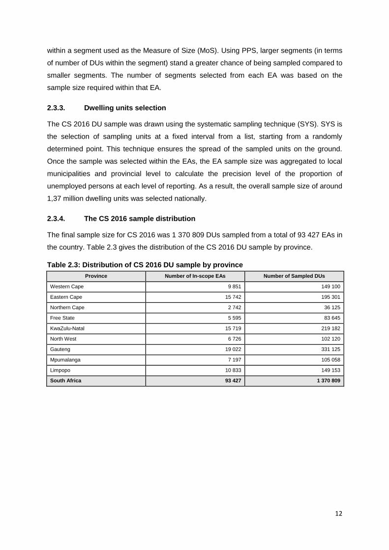
2.3.4. The CS 2016 sample distribution

The final sample size for CS 2016 was 1 370 809 DUs sampled from a total of 93 427 EAs in

the country. Table 2.3 gives the distribution of the CS 2016 DU sample by province.

Table 2.3: Distribution of CS 2016 DU sample by province

Province Number of In-scope EAs Number of Sampled DUs

Western Cape 9 851 149 100

Eastern Cape 15 742 195 301

Northern Cape 2 742 36 125

Free State 5 595 83 645

KwaZulu-Natal 15 719 219 182

North West 6 726 102 120

Gauteng 19 022 331 125

Mpumalanga 7 197 105 058

Limpopo 10 833 149 153

South Africa 93 427 1 370 809

13

3. The questionnaire

The questionnaire that was used for the CS 2016 was finalised following extensive research,

user consultations and testing to ensure that the questions asked met user requirements and

the key objectives of CS 2016.

3.1. Questionnaire development

A number of factors were considered when developing the CS 2016 questionnaire. These

included the impact on the respondent, the quality of the data collected and the length of the

questionnaire. The Census 2011 questionnaire content was used as a basis for the

development of the CS 2016 instrument. The decision to include new questions, any

modifications to existing questions and whether to remove any questions took into account a

number of factors such as user consultation feedback on importance of the data item, policy

needs, data quality, costs, historical comparability, respondent burden, operational

considerations and whether alternative data sources are available.

The CS 2016 questionnaire consisted of six main sections, 11 sub-sections and a total of

225 questions. A first draft of the paper questionnaire was developed in February 2015 and

various versions were reviewed and updated thereafter based on discussions with

stakeholders.

CS 2016 is the first national survey conducted by Statistics South Africa to use computer

assisted personal interviewing (CAPI) as the main data collection method. The electronic

CAPI version of the questionnaire was developed using the Survey Solutions application.1

The Survey Solutions application is a software developed by the World Bank for

development of CAPI questionnaires. Survey Solutions was chosen because of the ease

with which a questionnaire can be developed using the application, with no specialised

training or skills required to use the software. In addition, Survey Solutions allowed for in

built interviewer checks, automated routing and collection of additional data (for example,

capturing GPS coordinates for location of interview). The CAPI questionnaire was developed

and revised concurrently with the paper questionnaire. The final questionnaire was approved

in January 2016.

3.1.1. User consultation process

Interaction and discussions with users and stakeholders is a key element of the

questionnaire development process. Engaging with them allows Stats SA to better

1 See www.worldbank.org for more information on the Survey Solutions application.

14

understand and respond to the key priorities for development in society, determine the

reaction to proposed changes in the questionnaire and incorporate users’ inputs into the

design of the questionnaire. In addition, user consultations also serve as an advocacy tool,

allowing for a more informed understanding and increased support of CS 2016 activities

from key stakeholders.

Initial consultations with subject-matter specialists within Stats SA were held where their

data needs, the usability of the data items, the validity and reliability of response categories

and questions were discussed using the Census 2011 questionnaire as a starting point.

Based on this discussion a draft list of data items were compiled and presented to the Stats

SA provincial staff, who also provided their input. Discussions were then held with national

departments, such as the Department of Higher Education and Training, Environmental

Affairs, Water and Sanitation and Human Settlements, where questions specific to their

departmental priorities were discussed. In February and March 2015, provincial user

consultations were held in all nine provinces with key stakeholders including representatives

from provincial government departments, municipal offices, universities, research institutions

and the private sector. In addition, comments on the draft questionnaire were solicited from

academics and researchers working with census and survey data. An interactive web page

located on the Stats SA website was also developed for data users to provide comments

and inputs on the proposed CS 2016 topics.

3.2. Questionnaire testing

CS 2016 was the first national survey undertaken by Stats SA using CAPI as a mode of data

collection in place of the traditional paper-assisted personal interviewing (PAPI). Testing of

the CAPI questionnaire was a critical step in ensuring that the data collection instrument was

designed correctly to collect the data that was needed. Tight project time lines did not allow

for piloting of the survey instrument in a full-scale survey setting, however the questionnaire

was assessed in a variety of smaller tests. Both the paper-based and electronic

questionnaires were tested extensively in-house, before the CAPI version was formally

subjected to two main testing processes, the Behind-the-glass (BTG) tests and the

Integrated Test (the Integrated Test involved testing of the content and data collection

related procedures in their entirety). The main objectives of the tests were to establish the

following:

Duration of interviews, i.e. how long it took to complete the questionnaire across

varying respondent profiles.

The design and flow of the questions.

To identify any biases in the way questions were asked.

15

To identify any recall issues when responding to the questionnaire.

To get a sense of the challenges or difficulties that might arise in administering the

questionnaire using a tablet.

The sections below describe the two types of testing that were undertaken for the CS 2016

questionnaire.

3.2.1. Behind-the-glass tests

As the term suggests a BTG test is a process whereby a face-to-face interview is conducted

in a controlled environment. While the interview is conducted in one room between the

interviewer and respondent, observers in an adjacent room observe the interview usually

through a two-way mirror. Three BTG tests in total were conducted at different times during

development of the questionnaire. Respondents who participated in the BTG tests were

identified and recruited across various communities to ensure a diverse demographic and

socio-economic respondent profile. The interviewers and observers that participated in the

BTG tests were staff members involved in content development and operations for CS 2016.

This allowed for the key stakeholders in the development and administering of the

questionnaire to get a first-hand view of how the questionnaire fared in an interview setting

and the issues related to its administration. The responsibility of interviewers during the BTG

exercise was to conduct interviews focusing on the questions themselves, following the

validation rules (skipping instructions), layout and flow of the questions.

Both new and revised questions were tested as rigorously as possible to ascertain their

applicability and usefulness. Testing of each question, particularly the suitability of new data

items and the design was a crucial process in the development of the questionnaire. The

new questions covered areas such as emigration, levels of satisfaction and perceptions with

regards to basic municipal services, mode and duration of travel to educational institutions or

workplace, and agricultural activities undertaken by the households.

3.2.2. Integrated Test

The CS 2016 Integrated Test was undertaken during November and December 2015. This

was a small scale test with the aim of testing certain aspects of the survey operations in an

integrated manner in a typical survey field setting. A sample of 160 DUs was drawn within 38

EAs across two municipalities from the Brits/GaRankuwa area (i.e. City of Tshwane

Metropolitan municipality and Madibeng municipality). The area was chosen on the basis

that it covers different EA types and allowed for the testing of methodologies and operations

under varying conditions.

16

The CS 2016 draft questionnaire was used for the Integrated Test. For the purposes of the

Integrated Test, the reference night used in the questionnaire was revised to be within the

fieldwork period (i.e. the night between 31 October and 1 November 2015 was used). In

addition, other questions making reference to specific calendar periods were also revised so

that they are applicable for administering during the Integrated Test.

The Integrated Test questionnaires were administered electronically using android operated

tablets as planned for CS 2016. Overall, the findings from testing of the questionnaire during

the Integrated Test indicated minimum errors in the form of inconsistencies and missing

values on the data collected.

3.2.3. Overview of changes to the questionnaire based on the tests undertaken

During the BTG tests the questionnaire allowed for multiple households (within a DU) to be

enumerated on the same questionnaire. The initial questionnaire, allowed for two types of

rosters; the household and the person rosters. This, however, proved to be problematic in

terms of the enumeration process because it created multiple roster layers in the

questionnaire which led to fieldworker confusion. It was therefore decided that a census

mode questionnaire be used in cases of multiple households.2 This therefore meant that in

cases of multiple households within DUs, only one household would be enumerated on the

assigned questionnaire and a census mode questionnaire would be created and completed

for the additional households within this DU. The Map Reference Number (MRN) identifier

would be used to link the questionnaires, just like the barcode was used for paper based

questionnaires. Based on the BTG tests and Integrated Test, additional instructions were

added to the questionnaire, sections of the questionnaire were re-arranged and validation

rules were revised for the final questionnaire used in CS 2016.

3.3. Questionnaire content

The target population of the survey was all persons in the sampled dwelling who were

present on the reference night (i.e. the night between 6 and 7 March 2016). The final CAPI

questionnaire was made up of three person rosters. One roster was utilised for the person

information, one roster for emigration and one roster for mortality. Table 3.1: CS 2016

questionnaire structure3.1 below shows the structure utilised for the final CAPI

questionnaire.

2 The Census mode questionnaire is a blank questionnaire loaded onto the FWs tablet and is not linked to any of the

sampled DUs. The FW while completing the questionnaire will then link the Census mode questionnaire to the appropriate DU being enumerated.

17

Table 3.1: CS 2016 questionnaire structure

Name of section Description

Statistics Act No.6 of 1999 and prefilled hierarchical

geographical information

Brief description of the Statistics Act reminding respondents

about the confidentiality clause and the prefilled hierarchical

geographical information as per the sample

Particulars of dwelling

Location and description of dwelling unit. This section was

completed by the interviewer.

Person information

Questions on demographics, migration, general health and

functioning, parental survival, education, employment,

income and social grants and fertility. This section was

completed for all household members and visitors who were

present on the night of the 6/7th March 2016

Housing, household goods, services and crime, and

agricultural activities

Perception questions on satisfaction with basic service,

questions on housing, household goods and services, crime,

agricultural activities and food security

Emigration and mortality

Emigration: Questions on sex, age, country of residence and

year moved for each member of the household who have

emigrated to another country since March 2006 and are still

residing there

Mortality: Questions on sex, age, year and month of death

and maternal mortality for each member of the household

who passed away 12 months prior to the reference night of

the survey

Result codes and comments

Result code for each visit, date and time of next visit and

comments. This section was completed by the interviewer.

The CAPI questionnaire consisted of 120 questions with enabling conditions and 44

questions with validation conditions. For some questions, for example, country of birth,

automated lists of all the countries in the world, were uploaded on the CAPI questionnaire

designer to reduce capturing errors when specifying country of birth.

3.4. Questionnaire approval and finalisation process

The questionnaire went through a number of iterations of modification and approval at

various levels before the final questionnaire was approved. The draft questionnaire was

presented to the CS 2016 technical committee and was revised based on the committee’s

comments and inputs from the user consultation processes. The questionnaire was

approved by the technical committee in August 2015. This questionnaire was then presented

to the Population Statistics Council in October 2015 where the committee approved the

questionnaire for testing and made several inputs regarding the length of questionnaire and

recommended further consultation with subject-matter specialists.

The paper-based questionnaire was further revised based on these inputs and findings from

the tests and the final questionnaire was submitted to and reviewed by Stats SA’s

Questionnaire Clearance Committee (QCC) in January 2016. The QCC reviewed the overall

18

content of the questionnaire as well as proposed skips. It also made recommendations

regarding the wording of questions, grammar and general editing. The final approved

questionnaire from the QCC was then used to update the electronic questionnaire to be

used for CS 2016 CAPI data collection.

19

4. Fieldwork Operations

CS 2016 introduced a number of technological innovations in terms of how fieldwork

operations and data collection was implemented. The use of tablets and specialised

software for navigation to sampled DUs including CAPI enumeration during CS 2016 was

different from the conventional PAPI field operations survey processes. These innovations

greatly improved the timeliness, efficiency and cost effectiveness of field operations for CS

2016.

4.1. Training Approach

One of the key factors for a successful survey is the quality of the field training operations.

Training builds better communication skills, ensures consistent quality, improved focus,

produces more effective and productive efforts and clarifies the concepts and processes of

the survey to all field staff including Fieldworkers (FWs), the Fieldwork Supervisors (FWSs)

and district and provincial staff members.

A 3-tier cascade approach was implemented with national, provincial and district level

training being conducted. The duration of training was for 10 days at each level and the

training teams consisted of Head Office (HO), Provincial Office (PO) and District Office (DO)

personnel including Subject Matter Specialists (SMS) from all relevant work streams within

the organisation. Provincial trainers were trained at national level (including FOMs, PSCs,

etc.), who in turn trained the district trainers (i.e. FWSs and DSCs) at the provincial level.

District trainers would subsequently train fieldworkers in their respective districts. Trainees at

district level were recruited based on meeting the minimum requirements of having

completed at least Matric and be willing and able to attend training within their identified

areas. Overtraining was done at district level to ensure an adequate pool of trainees for

recruitment of fieldworkers (20% over training was targeted within each district).

4.1.1. Training methodology

A multi-pronged training method was used to train field staff. This entailed a combination of

instructor-led and practical methods. An instructor-led method of training was delivered using

presentation slides. It covered training content such as:

Publicity

Navigation

Enumeration procedures

Computer Aided Personal Interview (CAPI) methodology

Unpacking of multiple DUs at a point

20

Practical training was also given in the form of role plays and mock interviews between

trainees. Practical training also included a field practice session where trainees were given a

sample of DUs (not part of the CS 2016 main sample) to navigate to and enumerate. The

following methods, techniques, tools and aids were used during training:

Table 4.1: Methods and techniques used during training

Level of training Methods and Techniques Tools Aids Duration

National /

Provincial / District

Training

Instructor –led

Presentation

Video

Group discussions

Role play

Field practice

Simulation

Question and Answer

Evaluation Exercises

Laptop

Projector

Flip chart

Tablets

Presentation slides

Fieldworker manual

FWS/FW manual

User guide – how to

use the tablet

10 days

each

4.1.2. Training venues

Training at the national level was conducted at fully paid for conference venues which met all

the requirements conducive for training, and at the Provincial level training venues within the

provincial offices were utilised. At the District level, most venues were sourced free of charge

and some at a minimal cost. Although training venues at District level were free or low-

priced, great effort was put to ensure that these met the requirements conducive for training

such as, but not limited to, adequate space, availability, safety and security, basic amenities

such as water and sanitation, etc.

4.1.3. Quality control during training

The quality of training was carefully monitored to ensure quality and consistency at the

various levels. A Head Office Support Team (HOST) was set up to assist and monitor

training at the various provincial and district level training venues. The HOSTs had a set of

objectives and indicators that they needed to reflect on during the training proceedings. The

support team noted their findings, on a checklist they were provided with. The findings and

actions taken were communicated to all stakeholders and also documented for future

improvements. The team were required to perform the following tasks during training:

Ensure that the program is on track, trainers and trainees were available and the

required resources (such as projectors, adequate furniture, microphones, etc.) were

in place for a conducive learning environment;

Assist with training where necessary.

21

Evaluation of overall training in terms of the content, delivery of training material and

tools used for training.

Administer assessment exercises and invigilate during the assessments.

Another aspect of quality control during training was the administration of assessment

exercises aimed at measuring trainees’ knowledge, skill and aptitude towards fieldwork.

These assessments were used during the recruitment process to select the best performing

trainees.

4.2. Fieldwork approach

During fieldwork, the FWs were expected to use the tablet to navigate to points where the

sampled DUs allocated to them were located. Once at the point they were required to list the

DUs at that point and identify the sampled DUs from this listing using the Dwelling Unit

Record Form (DURF) loaded on the tablet. Once the sampled DU was identified they then

enumerated the DU using the CAPI questionnaire loaded on the tablet.

4.2.1. Process of navigating to sampled DUs

Go-survey was the application used to navigate to the geo referenced point where the

sampled DU was located. The tablet of each FW had the application with a built-in map with

the geo referenced points allocated to that specific FW so that they could keep track of

points in their work load. The application had an inbuilt GPS location system that guided the

FW in real time to the point they were navigating too.

4.2.2. Completion of DURF

The purpose of the DURF was similar to the listing summary book used in conventional

PAPI surveys. It was used to assist FWs in listing the DUs at a point (when there were

multiple DUs at that point) and identifying sampled DUs for enumeration from this listing. The

FWs completed the DURF by observing the actual structures at that the point on the ground

and listing them using a similar methodology to conventional listing approaches for surveys

at Stats SA.

4.2.3. Completion of questionnaire for households

The CS 2016 questionnaire was allocated to each sampled DU together with the DURF for

that particular DU and loaded on the tablet. Fieldworkers would digitally record all the

information of the members in a roster for a particular household in the CAPI questionnaire

22

loaded on the tablet. Completed questionnaires were submitted to supervision and quality

control twice a day using the synchronisation functionality on Survey Solutions. Where there

were multiple DUs and HHs identified, provision was made for additional questionnaires to

be available on the tablet (in the form of Census mode questionnaires). These

questionnaires were then linked to the main questionnaire through the MRN _ID identifier.

4.3. Quality control during fieldwork

A number of steps were taken during fieldwork to ensure quality of data being collected by

FWs. The first level of supervision and support in the field was the FWSs. Each FWS was

responsible for approximately 19 FWs. The FWS was responsible for managing all CS 2016

materials and resources in their respective FWS units. The FWS was also responsible for

supervision of FWs, quality assurance through remote monitoring and ensuring coverage of

the area assigned to them. Supervisors also monitored the progress of their FWs on a

continuous basis through a tablet using remote supervision software and intervened when

issues were picked up. FWSs reported to the DSCs in their area and had to submit daily

progress reports.

4.3.1. Role of DSCs

The DSCs were responsible for the final approval of the questionnaires coming from the field

in terms of completeness, accuracy and consistency. Approved questionnaires were

submitted electronically to the Head Office database where further checks were done.

Rejected questionnaires were sent back to FW tablets electronically and would appear on

the FWs tablet the next time they synchronised. The DSC was responsible for the

assignment of the workload to FWs and the reassignment of workloads when FWs resigned

or left work prior to the end of the data collection period. Payment of salaries to field staff

was triggered when the work done by the FW or FWS is complete and of acceptable quality

and the data collection tablet and field gear had been returned. The DSC was responsible

for signing off on payment for FWSs and FWs reporting to them.

4.3.2. Verification process for Out of Scope DUs

The Out of Scope Dwelling (OOS) units are those DUs that do not contain any households

as part of the target population and therefore no questionnaires and data can be collected

for these DUs. It is important to verify any DU that is classified as OOS by the FW (for

instance those DUs classified as vacant, demolished, unoccupied, new dwellings under

construction, misclassifications and unoccupied dwelling structures) since it contributes to a

decrease in the realised sample. DUs that were classified as OOS were verified by the FWS

and Head Office officials deployed to the districts. The verification process was done through

23

physical observation of the DU (actual visit to the DUs). After the OOS DUs were verified, a

verification form was signed by the FWS/Head Office official and submitted to the DSC for

approval of the questionnaire.

4.3.3. Handling of refusals

Surveys in general have to deal with a certain level of non-response. Households in some of

the sampled units might refuse to participate in the survey. It is important to have a strategy

to try and convince these households to participate in the survey, as a refusal leads to no

data being collected from an eligible household in the sample. For CS 2016, when the FW

encountered a refusal, they had to complete a refusal form to report it to their FWS, including

the physical address of the dwelling, contact details of the non-responding household or

respondent and the reasons for refusal (if possible).

The FWs were to report or inform the refusal to the FWSs. The message to the FWS was to

include the physical address of the DU and if possible the contact details of the

respondent(s) and the reasons as to why the respondent was refusing. The FWS would then

attempt to contact the household and elicit a response. If the household still refused, then

the matter was escalated to the DSC who issued a refusal letter to the respondent informing

them of the consequences of not responding in line with the Statistics Act of 1999. Many of

the households, after receiving the refusal letters made appointments with the district office

to be enumerated. For CS 2016 there were no cases that were reported to South African

Police Services (SAPS) for investigation regarding refusals.

Refusals could also occur at community level, where an entire community might not want to

participate for reasons such as staging a service delivery protest against the government or

a gated community (such as a town house complex) might not allow access to the complex.

Statistics South Africa had an enforcement strategy in place to deal with these types of

refusals. The strategy involved a coordinated effort between Statistics South Africa and key

stakeholders within the security enforcement agencies to provide assistance [the project was

registered with the National Joint Operation Committee (NATJOC)] as well as

communicating with community leaders, security management agencies, estate managers

and home owners associations prior to the beginning survey and during the survey to gain

their support.

24

5. Data management and data processing

The CS 2016 has enabled Statistics South Africa in using a technology-driven approach in

its operations. This implies that the flow of field operations has been dependant on different

systems using pre-prepared data (i.e. geo-referenced mapping information), the transaction

data (i.e. monitoring the field operations), the administration data and the statistical data (i.e.

related to the questionnaire). All the data sources mentioned above are inter-linked, thus

providing a support mechanism of control and efficient management of the full survey value

chain.

5.1. Data management

5.1.1. Database used

It is important to mention the data sources used as their inputs contribute in post-

enumeration data management. The sources of data used were:

- Geo-reference spatial frame used for sampling and field navigation through the Go-

survey system;

- Human resources recruitment system which provided the main source of

applicants fieldworkers (ESRI platform);

- Leaner Management system which provided the assessment of training and scoring

of successful candidates (SQL-server database);

- Survey Solutions application developed by the World Bank and used for CAPI,

interview management and data capturing (PostgreSQL database);

- Minimum Acceptance Rule (MAR) system applied in SQL server as tool of quality

management using minimum criteria (SQL server);

- SAS BI system providing the monitoring and performance management at each

level of fieldwork;

- SAS was used for structure edits, weighting, consistency edits and preliminary

analysis; and

- SuperCross is used for tabulation of data

During field operations, the different databases (i.e. CAPI and Go-survey) were updated

instantly using a mobile platform which synchronised information captured and the location

where the interview took place. On a daily basis, the data was manually exported from the

central repository cloud (CAPI and Go-Survey) to Stats SA Head Office servers as there

were no live links. The following files were exported:

CS2016Household_QN (Sampled household questionnaire)

25

CS2016Household_QN_CensusMode (Additional household questionnaire)

CS2016Persons (Persons in sampled household questionnaire)

CS2016Persons_CensusMode (Persons in additional household questionnaire)

CS2016Mortality (Death records in sampled household questionnaire)

CS2016Mortality_CensusMode (Death records in additional household

questionnaire)

CS2016Emigrant (Emigrants records in sampled household questionnaire)

CS2016Emigrant_CensusMode (Emigrants records in additional household

questionnaire)

interview_actions_Main (Transaction on sampled household questionnaire)

interview_actions_CensusMode (Transaction on additional household

questionnaire)

interview_comments_Main (Comments by fieldworkers on sampled household

questionnaire)

interview_comments_CensusMode (Comments by fieldworkers on additional

household questionnaire)

DURF_CS_2016_FINAL (Listing records of both sampled dwelling units (DU) and

additional dwelling unit)

interview_actions_DURF (Transaction on listing records)

interview_comments_DURF (Comments on listing records)

National_Samplepts_20160218 (DUs linked to map reference number as the

main sample)

The above datasets were exported into the following three streams of production:

The checking of minimum acceptability rule,

The SAS BI dashboard performance monitoring of the fieldwork, and

The final dataset for editing, weighting and analysis.

26

The following table provides the number of records associated with each of the input files:

Table 5.1: Number of records per input file for data processing

Table Name Number of

records Unit

CS2016Household_QN 1 370 811 Number of questionnaires

CS2016Household_QN_CensusMode 80 877 Number of questionnaires (Census mode)

CS2016Persons 3 228 724 Number of persons

CS2016Persons_CensusMode 170 324 Number of persons (Census mode)

CS2016Mortality 30 820 Number of deaths

CS2016Mortality_CensusMode 1 202 Number of deaths (Census mode)

CS2016Emigrants 6 314 Number of emigrants

CS2016Emigrants_CensusMode 609 Number of emigrants (Census mode)

interview_actions_CensusMode 724 508 Number of transactions (Census mode)

interview_actions_DURF 5 911 357 Number of transactions (DURF)

interview_actions_Main 11 588 716 Number of transactions (DURF)

interview_comments_CensusMode 215 909 Number of comments (Census mode)

interview_comments_DURF 321 897 Number of comments (DURF)

DURF_CS_2016_FINAL 1 303 180 Number of dwelling units

GeoHierarchy_EA2011_2016 (EAs) 103 576 Number of Enumeration Areas

5.1.2. Minimum acceptability rules (MAR)

Sample identification criteria:

The minimum acceptability rules was a procedure attempting to detect questionnaires

(households or persons) that may have been falsely or erroneous captured by the

fieldworkers. Every day, an export of all records in CAPI was loaded into SQL-server

database. The MAR procedure checked if there was minimum information allowing the

identification of the questionnaire (EA, map reference number, dwelling unit, household

number). Most importantly, the map reference number and the dwelling unit had to match

the sampled units. In addition, the procedure ascertained if the final result code was for a

responding household. In case of non-respondents, the procedure returned the

questionnaire to the field for a follow-up attempt to try and reduce non-response. In case of

out-of-scope dwellings, the procedure returned the questionnaire to the FWS for

confirmation of the out-of-scope status of the questionnaire.

Distance criteria:

In cases where the interview was indicated to have taken place far from the geographical

reference coordinates of the sampled DU (i.e. more than 30 metre radius), then the

fieldworker was requested (at least 4 times) to confirm if the interview was completed for the

correct sampled DU using two sources of information (i.e. Go-Survey navigation system and

27

Survey Solution CAPI captured geo-coordinates against the sampled geo-coordinates). The

distance was calculated using the Spherical Law of Cosines which provides accurate

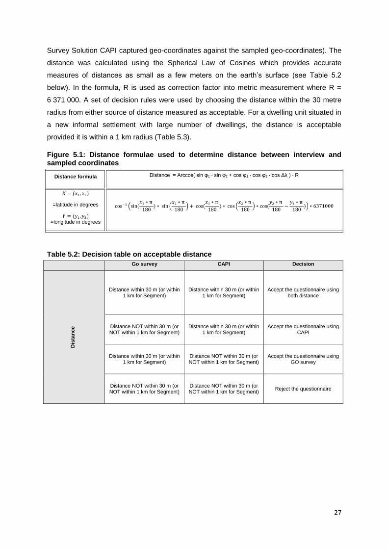
measures of distances as small as a few meters on the earth’s surface (see Table 5.2

below). In the formula, R is used as correction factor into metric measurement where R =

6 371 000. A set of decision rules were used by choosing the distance within the 30 metre

radius from either source of distance measured as acceptable. For a dwelling unit situated in

a new informal settlement with large number of dwellings, the distance is acceptable

provided it is within a 1 km radius (Table 5.3).

Figure 5.1: Distance formulae used to determine distance between interview and sampled coordinates

Distance formula Distance = Arccos( sin φ1 ⋅ sin φ2 + cos φ1 ⋅ cos φ2 ⋅ cos Δλ ) ⋅ R

𝑋 = (𝑥1, 𝑥2)

=latitude in degrees

𝑌 = (𝑦1, 𝑦2) =longitude in degrees

cos−1 (sin(𝑥1 ∗ π

180) ∗ sin (

𝑥2 ∗ π

180) + cos(

𝑥1 ∗ π

180) ∗ cos (

𝑥2 ∗ π

180) ∗ cos(

𝑦2 ∗ π

180−

𝑦1 ∗ π

180)) ∗ 6371000

Table 5.2: Decision table on acceptable distance

Go survey CAPI Decision

Dis

tan

ce

Distance within 30 m (or within 1 km for Segment)

Distance within 30 m (or within 1 km for Segment)

Accept the questionnaire using both distance

Distance NOT within 30 m (or NOT within 1 km for Segment)

Distance within 30 m (or within 1 km for Segment)

Accept the questionnaire using CAPI

Distance within 30 m (or within 1 km for Segment)

Distance NOT within 30 m (or NOT within 1 km for Segment)

Accept the questionnaire using GO survey

Distance NOT within 30 m (or NOT within 1 km for Segment)

Distance NOT within 30 m (or NOT within 1 km for Segment)

Reject the questionnaire

28

Household acceptability criteria:

The household record was considered as acceptable when it had the minimum number of

variables with responses. The household variables used for these criteria are grouped into

the following categories:

Category 1 (H06_TYPE OF MAIN DWELLING, H07_TENURE STATUS, H13_MAIN

SOURCE OF WATER, H21_TOILET FACILITY, H25_ACCESS TO ELECTRICITY,

H-32 REFUSE DISPOSAL), and

Category 2 (H-33 HOUSEHOLD GOODS, H-34 INTERNET SERVICES, H-39

INVOLVEMENT IN AGRICULTURAL ACTIVITIES).

The rule of acceptability used for a household record was that there should be at least two

valid responses in category 1 and two valid responses in category 2.

Person acceptability criteria:

The person record was considered as acceptable when it had the minimum number of

variables with responses. The person variable used for this criterion was grouped into the

following categories:

Category 1 (F01_PERSON NAME, F02_SEX, P01_DATE OF BIRTH OR F03_AGE,

P02_RELATIONSHIP TO HEAD OF HOUSEHOLD, P03_MARITAL STATUS,

P04_POPULATION GROUP), and

Category 2 (P08_PROVINCE OF BIRTH, P19a_MOTHER ALIVE, P19b_FATHER

ALIVE and P20_ATTENDANCE AT AN EDUCATIONAL INSTITUTION),

Category 3 (P-05_LANGUAGE, P-06_RELIGIOUS AFFILIATION/BELIEF, P-

27_EMPLOYMENT STATUS (P-27a, P-27b, P-27c)).

The rule of acceptability used for a person record was that there should be at least two valid

responses in category 1, at least two valid responses in category 2 and at least one valid

response in category 3. Note that particular attention was given to variables required for

calibration where any invalid value was returned to the field for correcting where appropriate.

The variables used for calibration were age (or date of birth), sex and population group.

29

5.2. Data processing of questionnaires

5.2.1. Transactional accounting from CAPI to SQL-server /SAS

The accounting of the questionnaires in the Survey Solutions system was tracked through

transaction stages. Therefore, a valid questionnaire should had in its transaction

“FirstAnswerSet” and “Completed” indicated. If a questionnaire had been accepted by the

MAR, it had to still go through the “ApproveBySupervisor” as an additional stage for

verification. If the questionnaire had been sent back to the fieldworker, it had as an additional

stage “RejectedBySupervisor” (Table 5.3).

Table 5.3: Transaction stages for the CAPI questionnaire

Stages

SupervisorAssigned

InterviewerAssigned

InterviewerAssigned

FirstAnswerSet

Restarted

Completed

ApproveBySupervisor

RejectedBySupervisor

RejectByHeadquarter

ApproveByHeadquarter

There were questionnaires that were assigned to fieldworkers but little or no information was

completed on them at the end of the fieldwork period and they were moved to the completed

stage (e.g. non-responses). Also, there were questionnaires that were returned to

fieldworkers for correction or to provide feedback but no response was received up until the

end of the data collection period (see Table 5.4). Overall, there were 1 454 674

questionnaires in CAPI, 1 370 809 corresponded to the sampled DUs and 83 865 as CS

2016 additional questionnaire (using census mode). However, the accounting of the final

export from CAPI to SQL server and SAS provided only 1 451 688 questionnaires (i.e. 2 986

questionnaires were not exported as they were without any information.

30

Table 5.4: Questionnaire accounted for at the end of field operations

CS 2016 MAIN sample

questionnaire (MAIN mode)

CS 2016 additional questionnaire

(Census Mode) Total questionnaire

Questionnaires assigned with little or no information collected

41 033 216 41 249

Completed questionnaires with no minimum acceptability rule applied

114 470 8 399 122 869

Rejected questionnaires using minimum acceptability rule without any feedback from fieldworkers

111 036 10 559 121 595

Approved Questionnaires using the minimum acceptability rule

1 104 124 64 440 1 168 564

Rejected by HQ without any feedback from fieldworkers

146 251 397

Total 1 370 809 83 865 1 454 674

5.2.2. Structural data editing

The process of structure edits was to make sure that the all survey questionnaires are

uniquely identifiable, valid and have the minimum acceptable criteria. The following steps

were undertaken during structural editing:

1. Combining the questionnaire datasets from the CS 2016 main survey mode with the

additional questionnaires in the census mode;

2. Correction of the key variables (i.e. map reference number (MRN_ID) and the

dwelling unit number (DUNo)). Specifically cleaning the misplacement of the digit

error, blank digit or use of underscore between digit when required;

3. Checking if map reference numbers and dwelling unit numbers matched the original

sample;

4. Determination of the distance between the visited points and the original sample

location geo-coordinates;

5. In cases where the distance was within 30 m radius, updating of any missing map

reference number and dwelling unit number were completed as determined to be

within nearby acceptable distance from the original sample points.

6. In cases where there was a new additional dwelling unit number at the sampled map

reference number, verification of the additional records captured in the dwelling unit

reference frame (DURF database) was undertaken;

7. Checking if there was an existence of multiple DU at valid sample points and

verifying if there were duplicate dwelling units or household numbers.

8. Checking if there were cases violating the MAR;

31

9. Determination of the FINAL RESULTS CODE per questionnaire (based on the

possibility of up to 4 visits at the household);

10. Determination of the usability of the questionnaire for subsequent statistical analysis

process where each questionnaire was classified as usable or not depending on

whether it matched the original sample, it was within the nearby acceptable distance

and it had the minimum acceptable number of responses;

11. The validation of different records by checking the unique ID, the fact that one

household should have at least a person or more; that the emigrants’ records or

mortality’s records are associated to one unique household.

Table 5.5 matches the original sample against the questionnaires received. Distance was

used as supporting criteria in order to be able to match the sample in case the primary keys

had been changed in error by the fieldworker. In addition, only the completed questionnaires

with valid information are used for weighting and tabulation (see Table 5.6 below). There

were some completed questionnaires which were excluded because they did not match the

sample, lacked minimum acceptable criteria or were far from the geo-reference point (i.e.

these questionnaires could not be reconciled with the CS 2016 sample).

Table 5.5: Questionnaire records after MAR

Survey Mode MAR status Distance in

metres

No weights

calculated

Weights

calculated Total

CS additional

questionnaire

(census mode)

Acceptable Minimum

criteria

<=30 12 509 51 164 63 673

>30 8 66 74

Not acceptable minimum

criteria

<=30 17 006 17 006

>30 124 124

CS main

sampled

questionnaire

(main mode)

Acceptable Minimum

criteria

<=30 2 719 843 033 845 752

>30 708 90 364 91 072

Not acceptable minimum

criteria

<=30 342 753 342 753

>30 91 234 91 234

Total 467 061 984 627 1 451 688

Note that there were 184 households with invalid information on at least one of the key

demographic variables required for calibration and therefore these were excluded from the

household weighted file.

32

Table 5.6: Questionnaire records after structural editing

Responding

categories Final results code

No weights

Weights allocated

Weights allocated

Total CS additional

questionnaire

(Census

Mode)

CS main

sampled

questionnaire

(Main Mode)

CS additional

questionnaire

(Census

Mode)

CS main

sampled

questionnaire

(Main Mode)

Responses 11 Completed 12 988 6 057 50 913 928 904 998 862

12 Partly completed 398 2 278 317 4 493 7 486

Non-

responses

21 Non-Contact 3 001 50 900 53 901

22 Refusal 1 393 36 345 37 738

23 Other Non-Contact 314 7 658 7 972

Out of scope

31 Unoccupied dwelling 3 762 97 731 101 493

32 Vacant dwelling 1 545 48 978 50 523

33 Demolished 591 33 777 34 368

34 New Dwelling Under

Construction 241 9 562 9 803

35 Status change 455 11 412 11 867

36 Frame error 1 576 73 654 75 230

No results provided

(BLANK) 3 383 59 062 62 445

Total 29 647 437 414 51 230 933 397 1 451 688

5.2.3. Consistency data editing

The strategy for ensuring consistency editing was to check consistency within the thematic

section of the questionnaire only key variables. The Survey Solutions system also allowed

validation rules to be built in at the time of interview which minimised the number of

consistency edits required at this stage. Therefore, most of the edits at this stage dealt with

“unspecified” cases or for derived variables.

There was however some imputation of variables with extreme errors or inconsistencies

forced by the fieldworkers. The CS 2016 analysis report will elaborate more on these

variables. The edits rules applied were mostly deduced directly from the logic consistency

between different variables (i.e. logical imputation). There are however few cases where

dynamic imputation methods were used where additional deduction of information was made

from a matrix of predicting variables by borrowing the information from valid records to

update those records without valid information (i.e. hot deck imputation).

The other aspects of consistency edits are the derived variables. For instance, the

geographical distribution of population or household is determined using the map reference

number which is associated to the geo-reference coordinate points feature representing the

33

dwelling unit. Therefore, the aggregated counts linked to the derived variables of the local

municipalities, district municipalities and provinces. There are important derived variables

such as age which was directly derived from the date of birth at person level.

5.3. Edited Data Files

The final data files are representative of the different statistical unit of observation as per the

questionnaire. The following are the different final records to be used for tabulation and

analysis in SAS.

Table 5.7: Number of records per final edited data file

Final Dataset in SAS Number of records

CS2016_PERSON_WEIGHTED20160627 3 328 867

CS2016_MORTALITY_WEIGHTED 30 064

CS2016_HOUSEHOLD_WEIGHTED 98 4627

CS2016_EMIGRANTS_WEIGHTED 5 205

CS2016_PERSON_AUDITTRAIL 14 788 329

CS2016_MORTALITY_AUDITTRAIL 2 309

CS2016_EMIGRANTS_AUDITTRAIL 658

CS2016_HOUSEHOLD_AUDITTRAIL 832 205

34

6. Sample Realisation

Post the data collection and structural editing process, the household and person files were

made available for the calculation of sample weights. Prior to the weighting process, it is

important to verify the number of records (i.e. DUs and HHs enumerated) on the data files

received against the actual sampled DUs on the initial sample file. This will allow for each

record on the DU sample file to be reconciled with data returning from the field and will also

assist in correctly accounting for each of the sample records during the weighting process.

The household file received for weighting had 1 434 884 household records after structural

editing was completed. The file was taken through a process of checks to ensure that there

were no missing, invalid or duplicate identifiers for each record on the file. The household

records were then validated against the DU sample file to link each of the valid households

to their sampled DUs, and identify and remove any erroneously enumerated households (i.e.

households enumerated but had no corresponding sampled DUs). Finally, the household file

was compared against the person file to validate that all respondent households had

corresponding valid person records in the person file. Respondent households with no

persons matching on the person file were recoded to non-respondent households. The final

household file used for weighting was made of 1 422 928 records. The final result codes for

each record were mapped to one of the three final response status categories as shown in

Table 6.1 where 1=Respondent (i.e. having a completed or partly completed questionnaire

for the household), 2=Non-respondent (i.e. where the household did not respond and/or

there was no questionnaire completed), and 3=Out-of-scope (i.e. where no eligible

household was found to be enumerated).

Table 6.1: Mapping of the final result codes to the response categories

Final Result Code Label Frequency Percentage

11 Complete 979 967 68,87

12 Partly complete 4 811 0,34

21 Non-contact 51 918 3,65

22 Refusal 36 807 2,59

23 Other non-response 7 724 0,54

24 ‘Empty Households’ - Responding households without valid persons

(assigned during data preparation for weighting). 797 0,06

25

Sampled DUs without corresponding dwelling on household file

(assigned during data preparation for weighting). 5 925 0,42

31 Unoccupied dwelling 98 693 6,94

32 Vacant dwelling 49 367 3,47

33 Demolished dwelling 33 886 2,38

34 New Dwelling Under Construction 9 638 0,68

35 Status change 11 568 0,81

36 Classification error 74 287 5,22

Missing or invalid Missing or Invalid Code 57 540 4,04

Total 1 422 928 100,00

35

6.1. Out-of-scope (OOS) rate

The out-of-scope (OOS) rate is defined as the proportion of DUs in which no eligible

household was found to the total number of sampled dwelling units (including any additional

DUs identified during data collection). There are several reasons why dwelling units may not

contain eligible households. At the time of enumeration the dwelling unit could have been

vacant or unoccupied, the dwelling unit could have been demolished or converted into a

shop, or the structure could have been erroneously classified as a dwelling unit on the

frame.

Let 𝑑𝑔 be the total number of dwelling units, sampled from the geographic area g and

𝑑𝑔(𝑜𝑠)

the corresponding number of dwelling units with no eligible household. The OOS rate

for geographic area g is then given by:

𝑂𝑢𝑡 𝑜𝑓 𝑆𝑐𝑜𝑝𝑒 𝑅𝑎𝑡𝑒𝑔 =𝑑𝑔

(𝑜𝑠)

𝑑𝑔× 100 (2)

Table 6.2 lists the OOS rates for CS 2016 nationally and provincially (see Appendix B for

OOS rates at local municipality level).

Table 6.2: National and provincial level OOS rates

Province OOS Rate

Western Cape 27,79

Eastern Cape 29,99

Northern Cape 33,74

Free State 24,79

KwaZulu-Natal 17,58

North West 24,90

Gauteng 21,49

Mpumalanga 25,63

Limpopo 25,51

South Africa 24,29

Nationally, the OOS rate for CS 2016 was 24,29%, which is high relative to other surveys

conducted by Statistics South Africa using the conventional Master Sample listings (for

example, the OOS rate for QLFS quarter 1 of 2016 was 16,11% nationally). The high OOS

rates could be due to quality of the geo-referenced dwelling frame used for CS 2016.

Although an update process was conducted to improve the quality of the Dwelling Frame

prior to its use in CS 2016, the high OOS rates are indicative that the frame required a more

intensive verification of the classification of DUs. Going forward, the verification of the frame

is an important step for future surveys that will be using the geo-referenced dwelling frame.

Most provinces also experienced similar OOS rates. However, the Northern Cape and

Western Cape had relatively higher OOS rates at 33,74% and 27,79% respectively.

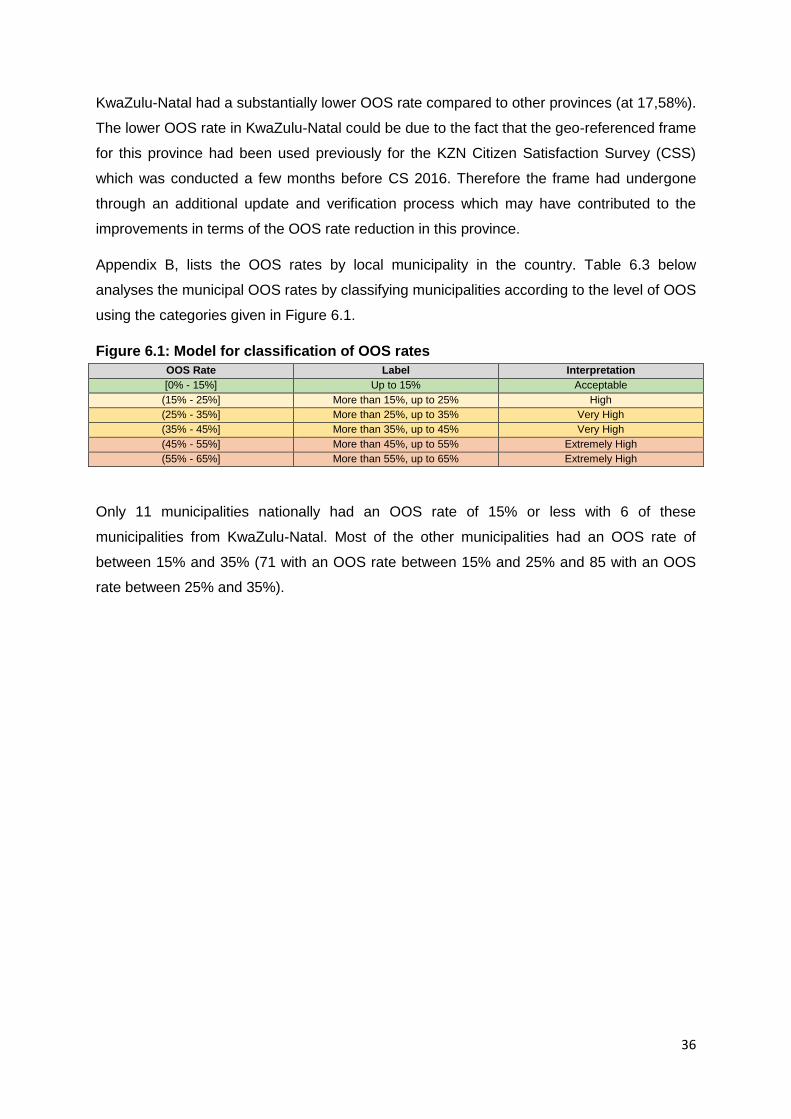
36

KwaZulu-Natal had a substantially lower OOS rate compared to other provinces (at 17,58%).

The lower OOS rate in KwaZulu-Natal could be due to the fact that the geo-referenced frame

for this province had been used previously for the KZN Citizen Satisfaction Survey (CSS)

which was conducted a few months before CS 2016. Therefore the frame had undergone

through an additional update and verification process which may have contributed to the

improvements in terms of the OOS rate reduction in this province.

Appendix B, lists the OOS rates by local municipality in the country. Table 6.3 below

analyses the municipal OOS rates by classifying municipalities according to the level of OOS

using the categories given in Figure 6.1.

Figure 6.1: Model for classification of OOS rates

OOS Rate Label Interpretation

[0% - 15%] Up to 15% Acceptable

(15% - 25%] More than 15%, up to 25% High

(25% - 35%] More than 25%, up to 35% Very High

(35% - 45%] More than 35%, up to 45% Very High

(45% - 55%] More than 45%, up to 55% Extremely High

(55% - 65%] More than 55%, up to 65% Extremely High

Only 11 municipalities nationally had an OOS rate of 15% or less with 6 of these

municipalities from KwaZulu-Natal. Most of the other municipalities had an OOS rate of

between 15% and 35% (71 with an OOS rate between 15% and 25% and 85 with an OOS

rate between 25% and 35%).

Table 6.3: Distribution of municipal OOS rates by category

Province Out-of-Scope Rate (OOSR) Categories

Overall OOSR ≤ 15% 15% < OOSR ≤ 25% 25% < OOSR ≤ 35% 35% < OOSR ≤ 45% 45% < OOSR ≤ 55% 55% < OOSR ≤ 65%

Western Cape 0 6 6 5 7 1 25

Eastern Cape 0 4 15 14 5 1 39

Northern Cape 1 3 6 8 4 5 27

Free State 2 4 6 3 4 1 20

KwaZulu-Natal 6 29 16 0 0 0 51

North West 0 6 8 5 0 0 19

Gauteng 2 3 5 0 0 0 10

Mpumalanga 0 7 9 2 0 0 18

Limpopo 0 9 14 1 0 1 25

South Africa 11 71 85 38 20 9 234

There were 29 municipalities nationally with extremely high OOS rates, with 9 of them with an OOS rate of between 55% and 65%. Table 6.4

below lists these 9 municipalities with their extremely high OOS rates. Prince Albert local municipality in the Western Cape had the highest

OOS rate at almost 65%, while 5 municipalities in the Northern Cape (Kareeberg, Karoo Hoogland, Hantam, Khâi-Ma and Ubuntu) had extreme

OOS rates of above 58%. Note that high OOS rates do not impact on the quality of the data collected from the field, however, it is an indicator

of the quality of the sample frame used and reduces the effective sample size, and therefore the precision level of estimates within given

domains.

Table 6.4: Top 9 Municipalities with Extremely High OOS Rates

6.2. Response rate

The response rate is defined as the proportion of eligible households which completed a

questionnaire with usable information to the total number of eligible households in the survey

including non-respondent households (i.e. eligible households for which a questionnaire was

not completed). There are many different reasons for household non-response; for example

members of the particular household might refuse to participate in the survey, or the

household could not be contacted during the data collection period, or the household did not

provide usable information, etc.

Let 𝑛𝑔 be the number of eligible households from the geographic area g and 𝑛𝑔𝑟 the

corresponding number of respondent households (where eligible households include both

respondent and non-respondent households, but exclude out-of-scope households). The

response rate is then given by:

𝑅𝑒𝑠𝑝𝑜𝑛𝑠𝑒 𝑅𝑎𝑡𝑒𝑔 =𝑛𝑔

𝑟

𝑛𝑔× 100 (3)

Figure 6.2 illustrates a model that is used to determine the minimum acceptable level of

response for surveys conducted by Stats SA for household based surveys.

Figure 6.2: Model for response rates

Response Rate Label Interpretation

[80% - 100%] 80% or Higher Acceptable

[60% - 80%) 60% up to 80% Low

[40% - 60%) 40% up to 60% Extremely Low

Table 6.5 lists the response rates for CS 2016 nationally and provincially (see Appendix B

for response rates at local municipality level).

Province Municipality Out-of-Scope Rate

Western Cape Prince Albert 64,99

Northern Cape Kareeberg 64,72

Northern Cape Karoo Hoogland 63,51

Eastern Cape Baviaans 61,00

Northern Cape Hantam 59,22

Northern Cape Khâi-Ma 58,57

Northern Cape Ubuntu 58,51

Limpopo Mookgopong 58,11

Free State Tokologo 56,30

39

Table 6.5: National and provincial level response rates

Province Response Rate

Western Cape 76,02

Eastern Cape 95,01

Northern Cape 89,72

Free State 90,74

KwaZulu-Natal 95,51

North West 91,59

Gauteng 87,25

Mpumalanga 92,00

Limpopo 97,21

South Africa 90,52

Nationally, the response rate for CS 2016 was 90,52% which was well within the minimum

acceptable threshold of 80% response rate. Across most provinces, the response rates were

also above the minimum acceptable criteria except for the Western Cape where the

provincial response rate was 76,02%. Appendix B, lists the response rates by local

municipality in the country.

Table 6.6 below analyses the municipal response rates by classifying them based on the

model above. Almost all municipalities achieved a response rate of 80% or higher nationally

(222 of 234 municipalities).

Table 6.6: Distribution of municipal response rates by category

Province Response Rate (RR) Categories

Overall RR ≥ 80% 60% ≤ RR < 80% 40% ≤ RR < 60%

Western Cape 20 4 1 25

Eastern Cape 38 1 0 39

Northern Cape 24 3 0 27

Free State 20 0 0 20

KwaZulu-Natal 51 0 0 51

North West 17 2 0 19

Gauteng 10 0 0 10

Mpumalanga 18 0 0 18

Limpopo 24 1 0 25

South Africa 222 11 1 234

There were 11 municipalities which achieved a response rate of between 60% and 80% (low

response rate) while one municipality in the Western Cape achieved an extremely low

response rate. Table 6.7 below lists these 12 municipalities with low to extremely low

response rates.

40

Table 6.7: 12 Municipalities with low and extremely low response rates

Province Municipality Response Rate

Western Cape Stellenbosch 45,63

Northern Cape Hantam 64,10

Eastern Cape Sundays River Valley 68,08

Western Cape Drakenstein 71,45

Western Cape City of Cape Town 71,65

North West Tlokwe City Council 72,70

Northern Cape Karoo Hoogland 74,37

North West Kgetlengrivier 75,42

Western Cape Knysna 76,90

Limpopo Mookgopong 77,40

Northern Cape Thembelihle 78,05

Western Cape Mossel Bay 79,82

Stellenbosch municipality in the Western Cape achieved a substantially lower response rate

(45,63%) compared to other municipalities nationally. Of the 11 other municipalities with low

response rates (i.e. between 60% and 80%) four of them were from Western Cape (namely,

Drakenstein, City of Cape Town Metro, Knysna and Mossel Bay).

6.3. Classification of municipalities based on response rates and out of scope matrix

High non-response rates reduce the achieved sample and will result in increased variance of

survey estimates. In addition, if non-respondents are different from respondents based on

the characteristic of interest this will also lead to an increase in the bias of survey estimates.

Assuming the sampled DUs were correctly classified as out-of-scope, a high OOS rate will

also reduce the achieved sample size and increase the variance of the survey estimates in

the given domain.

41

Figure 6.3: Classification of municipalities based on response rate and out of scope matrix

Looking at the response rate and OOS rate together for each municipality and classifying

them based on the matrix given in Figure 6.3 above, we find that 11 municipalities have an

acceptable level of response rate as well as OOS rates. These municipalities are listed in

Table 6.8 below.

11 Municipalities

211 Municipalities

12

Municipalities

High Response

Rate

High Out-of-Scope

Rate

Low Out-of-Scope

Rate

Low Response

Rate

42

Table 6.8: 11 Municipalities with acceptable levels of response rates and OOS rates

Province Municipality Response Rate Out-of-Scope Rate

KwaZulu-Natal Greater Kokstad 97,55 8,95

KwaZulu-Natal Dannhauser 97,29 13,29

KwaZulu-Natal Newcastle 95,40 10,30

KwaZulu-Natal The Msunduzi 93,91 13,17

Gauteng Emfuleni 93,54 11,89

Gauteng Ekurhuleni 93,53 14,71

KwaZulu-Natal eThekwini Metro 92,97 12,21

KwaZulu-Natal Ubuhlebezwe 92,73 11,83

Free State Matjhabeng 89,54 13,28

Northern Cape Sol Plaatjie 88,56 12,65

Free State Mangaung 84,44 14,70

Most of the remaining municipalities (211) fell within the second quadrant with acceptable

levels of response rates but high levels of OOS rates. There were 12 municipalities who fell

in the third quadrant achieving low levels of response and having high OOS rates. These

municipalities are listed in Table 6.9 below.

Table 6.9: 12 municipalities with low levels of response rates and OOS rates

Province Municipality Response Rate Out-of-Scope Rate

Western Cape Mossel Bay 79,82 47,14

Northern Cape Thembelihle 78,05 30,35

Limpopo Mookgopong 77,40 58,11

Western Cape Knysna 76,90 39,93

North West Kgetlengrivier 75,42 28,47

Northern Cape Karoo Hoogland 74,37 63,51

North West Tlokwe City Council 7270 16,17

Western Cape City of Cape Town 71,65 23,94

Western Cape Drakenstein 71,45 23,12

Eastern Cape Sundays River Valley 68,08 31,94

Northern Cape Hantam 64,10 59,22

Western Cape Stellenbosch 45,63 20,28

NB: In order to fully understand the relationship as shown in Figure 6.3 above, between the

response rates and OOS rates for municipalities in each of the four quadrants, we

recommend that this analysis be read in conjunction with the report from the CS 2016

Evaluation Survey which was intended to assess under coverage and other non-sampling

errors during CS 2016.

43

7. The Sample Weights

The main goal of CS 2016 is to produce estimates of key indicators at local municipality

level. The sample was designed such that direct survey estimates for these indicators could

be produced at municipal level. The weighting approach is based on the sample design. This

chapter describes the approach that was used to determine the design weights for sampled

DUs, including the additional DUs that were not on the sampling frame initially but were

enumerated. The chapter also describes the adjustment factors applied to the design

weights to account for the excluded population from the sampling frame (from small EAs

excluded from the frame), non-response, and benchmarking to the known local municipality

population and household control totals.

7.1. Design weights

Based on the sample design, EAs on the sampling frame were either segmented or non-

segmented (see chapter on The Sample above). The design weights for segmented and

non-segmented EAs are different since they are treated differently during the sample design.

7.1.1. Design weights for sampled dwelling units

The design weight for each sample unit is derived during the sample design process. For

non-segmented EAs the design weight is equal to the inverse of the probability of selection

(i.e. inverse of the sampling rate (ISR)). The probability of selection for DUs within non-

segmented EAs is given by:

𝜋𝑖𝑗 =𝑛𝑖

𝑁𝑖 (4)

Where 𝜋𝑖𝑗 is the probability of the jth DU in non-segmented EA i being selected, 𝑛𝑖 is the

number of sampled DUs in non-segmented EA i and 𝑁𝑖 is the total number of DUs in non-

segmented EA i.

Within segmented EAs, a sample of one or more of the segments in the EA was selected

with probability proportional to the number of DUs in the segments (PPS) and then a sample

of DUs in the selected segments was taken. Therefore the probability of selection for DUs

within segmented EAs is given by:

𝜋𝑖𝑘𝑗 =𝑠𝑖×𝑛𝑖𝑘

𝑁𝑖 (5)

Where 𝜋𝑖𝑘𝑗 is the probability of the jth DU in segment 𝑘 of segmented EA i being selected, 𝑠𝑖

is the number of segments sampled from segmented EA i, 𝑛𝑖𝑘 is the number of sampled

44

DUs selected in segment k of segmented EA i and 𝑁𝑖 is the total number of DUs in

segmented EA i.

The design weight is then defined as the inverse of the probability of selection at the EA

level, accounting for the selection of all the sampling units, i.e. the selection of segments

from segmented EAs and the selection of DUs within selected segments as well as the

selection of DUs within non-segmented EAs as denoted below.

𝑊𝑑 = {

1

𝜋𝑖𝑗 ; 𝑁𝑜𝑛 − 𝑠𝑒𝑔𝑚𝑒𝑛𝑡𝑒𝑑 𝐸𝐴𝑠

1

𝜋𝑖𝑘𝑗 ; 𝑆𝑒𝑔𝑚𝑒𝑛𝑡𝑒𝑑 𝐸𝐴𝑠

(6)

7.1.2. Design weights for additional dwelling units

During enumeration, additional dwelling units were identified and enumerated that did not

appear on the sampling frame. These additional DUs are in scope as part of the target

population for CS 2016. However, they did not have a chance of being selected into the

sample since they did not appear on the sampling frame. In order to properly account for

these additional DUs in the estimates, they would need to receive a weight in relation to the

conditional probability that one or more of the DUs on the frame at the same point were

selected into the sample.

Additional DUs were only considered to be eligible if they satisfied the following criteria:

(1) The additional DU was within one of the points that were part of the CS 2016 sample, or

(2) The additional DU had a DU number greater than the DU Count on the frame for the

given point.

The criteria above ensured that DUs erroneously enumerated were not included during the

weighting process. Criterion (1) ensured that those DUs that were not within any of the

points on the sample were excluded and Criterion (2) ensured that non-sampled DUs (from

the frame) within the points on the sample were excluded.

7.1.2.1. Non-segmented EAs

For non-segmented EAs where all DUs within the EA were selected into the sample (i.e.

take all EAs), the additional DUs identified would also appear in the sample with certainty

and therefore are assigned a design weight of 1.

𝑊𝑎𝑑𝑑 = 1 ; 𝑓𝑜𝑟 𝑎𝑑𝑑𝑖𝑡𝑖𝑜𝑛𝑎𝑙 𝐷𝑈𝑠 𝑖𝑛 𝑡𝑎𝑘𝑒 𝑎𝑙𝑙 𝐸𝐴𝑠 (7)

45

For non-segmented EAs where a sample of DUs within the EA was selected, if the number

of DUs on the sampling frame for that point was greater than or equal to the sampling rate

(or interval) that was applied in that EA, then the point would appear in the sample with

certainty (since at least one DU within that point would have been part of the sample).

Therefore any additional DUs linked to that point would also appear in the sample with

certainty and have a design weight of 1.

𝑊𝑎𝑑𝑑 = 1 ; 𝐹𝑜𝑟 𝑝𝑜𝑖𝑛𝑡𝑠 𝑤ℎ𝑒𝑟𝑒 𝑛𝑢𝑚𝑏𝑒𝑟 𝑜𝑓 𝐷𝑈𝑠 𝑜𝑛 𝑡ℎ𝑒 𝑓𝑟𝑎𝑚𝑒 ≥ 𝑠𝑎𝑚𝑝𝑙𝑖𝑛𝑔 𝑟𝑎𝑡𝑒 (8)

For those EAs where the number of DUs on the sampling frame for a point in the sample is

less than or equal to the sampling rate or interval, then the additional DUs at that point would

have been in the sample if any of the DUs on the frame were in the sample. Therefore the

design weight assigned to these additional DUs will be the design weight of the sampled

DUs (see (4) above) divided by the total number of DUs at this point on the sampling frame,

as given below.

𝑊𝑎𝑑𝑑 =𝑊𝑑

𝑁𝑖𝑟 ; 𝐹𝑜𝑟 𝑝𝑜𝑖𝑛𝑡𝑠 𝑤ℎ𝑒𝑟𝑒 𝑛𝑢𝑚𝑏𝑒𝑟 𝑜𝑓 𝐷𝑈𝑠 𝑜𝑛 𝑡ℎ𝑒 𝑓𝑟𝑎𝑚𝑒 < 𝑠𝑎𝑚𝑝𝑙𝑖𝑛𝑔 𝑟𝑎𝑡𝑒 (9)

Where:

𝑊𝑎𝑑𝑑 = Design weight assigned to additional DUs.

𝑊𝑑 = Design weight of the sampled DUs (see (6) above)

𝑁𝑖𝑟 = the total number of DUs on the sampling frame for point r in EA i.

7.1.2.2. Segmented EAs

Within segmented EAs, a two-stage PPS design was implemented, where one or more

segments within an EA was sampled with PPS and at the second stage a sample of DUs

was selected within the sampled segments. Each segment in an EA had one point with the

count of the number of DUs within that segment. Therefore the design weight assigned to

additional DUs within a sampled segment will be equal to the inverse of the probability of

selection for that segment, as given below.

𝑊𝑎𝑑𝑑 =𝑁𝑖

𝑠𝑖×𝑁𝑖𝑘 (10)

Where:

𝑁𝑖 = Total number of DUs from the sampling frame within EA i

𝑠𝑖 = Number of sampled segments within EA i

𝑁𝑖𝑘 = Total number of DUs from the sampling frame within segment k in EA i

46

7.2. Design weight adjustments

7.2.1. Synthetic weight adjustment

During the design of a sample, it is common practice to adopt the strategy of excluding very

small EAs from the sampling frame to improve operational efficiency during the survey.

These small EAs were excluded on the basis of cost and the feasibility to conduct field

operations within these areas as they are usually very remote and are sparsely populated.

However, these excluded EAs form part of the target population and therefore have to be

accounted for during the weighting process to reduce any bias due to coverage error in the

estimates due to their exclusion.

A synthetic adjustment factor to account for the contribution from the excluded DUs were

applied to the design weights. The adjustment factor is calculated using the DU counts at the

geographic area level within the local municipalities to reduce the risk of potential synthetic

bias. Let 𝑁𝑚𝑔 be the number of DUs within the target population from the 𝑔𝑡ℎ geographic

area within the 𝑚𝑡ℎ local municipality and 𝑁𝑚𝑔𝑓

the corresponding number of DUs on the

sampling frame. Then the synthetic weight adjustment factor that was used (by local

municipality and geographic area) is given by:

𝑆𝑦𝑛𝑡ℎ_𝑊𝑔𝑡𝑚𝑔 =𝑁𝑚𝑔

𝑁𝑚𝑔𝑓 (11)

7.2.2. Non-response adjustment

In order to account for unit non-response during surveys, an adjustment is usually made to

the design weights based on the assumption that the characteristics of responding units are

similar to those of the non-responding units within adjustment cells.

The non-response adjustment factor is defined as the ratio of the eligible units, i.e.

respondent and non-respondent units in the sample, to the respondent units. The adjustment

for total non-response was computed at two levels of non-response; at EA non-response

and household non-response levels. Non-response at EA level occurs when an EA has

eligible DUs but there are no responding HHs within the entire EA. While household level

non-response occurs when a particular household in an eligible EA does not respond.

47

7.2.2.1. EA non-response adjustment

The EA non-response adjustment factor will be based on the classification of EAs into one of

the three response categories. The classification of the EAs will be based on the

classification of the DUs and their households within the respective EAs in the following

manner:

Responding EAs:

o EAs that have at least one eligible DU with a responding household;

Non-Responding EAs

o EAs that have eligible DUs but with no responding households;

Out-of-Scope EAs

o EAs that have no eligible DUs.

The EA non-response adjustment factor will be defined as the ratio of the total sum of

weights within the respondent and non-respondent EAs and the sum of weights within the

respondent EAs at geographic level within the Local Municipality. Let 𝑝𝑔𝑚𝑟 be the sum of

weights within the respondent EAs from the 𝑔𝑡ℎ geographic area within the 𝑚𝑡ℎ local

municipality and 𝑝𝑔𝑚𝑛𝑟 the corresponding sum of weights within the non-respondent EAs. The

EA non-response adjustment factor at geographic area within the local municipality will be

defined as:

𝐸𝐴_𝑁𝑅_𝐴𝐷𝐽𝑔𝑚 =(𝑝𝑔𝑚

𝑟 +𝑝𝑔𝑚𝑛𝑟 )

𝑝𝑔𝑚𝑟 (12)

7.2.2.2. Household non-response adjustment

The household records were assigned to one of three response categories; responding, non-

responding or out-of-scope households. Only the in-scope household records will contribute

in computing the household non-response adjustment factor. The in-scope households are

all responding and non-responding households from the eligible DUs. The adjustment was

computed at EA level.

Let 𝑝𝑖 be the weighted number of eligible households in the dwelling sample from EA 𝑖 and

𝑝𝑖𝑟 be the weighted number of responding households from EA 𝑖 (segmented or non-

segmented EA). The household non-response adjustment factor will be defined as:

𝐻𝐻_𝑁𝑅_𝐴𝐷𝐽𝑖 =𝑝𝑖

𝑝𝑖𝑟 (13)

48

7.2.3. Adjusted design weight

The adjusted design weight for analysis (𝑊𝑎) will be defined as a product of the design

weight and the adjustment factors described above, i.e. synthetic weight adjustment and

non-response adjustment factors at EA and household level.

𝑊𝑎 = 𝑊𝑑 × 𝑆𝑌𝑁𝑇𝐻_𝑊𝐺𝑇𝑚𝑔 × 𝐸𝐴_𝑁𝑅_𝐴𝐷𝐽𝑚𝑔 × 𝐻𝐻_𝑁𝑅_𝐴𝐷𝐽𝑖 (14)

7.3. Calibration

The final step undertaken in constructing the sample weights at person and household level

for CS 2016 was to calibrate the adjusted design weights such that the respective aggregate

totals matched the distribution of the population across key demographic variables (i.e. age,

gender and population group) nationally, provincially and at municipal level. The control

totals used for this calibration process were independently derived by the Demography

Division at Stats SA using demographic models. The calibration cells were defined based on

the distribution of the survey data to avoid defining cells that may be too sparse (i.e. little or

no survey data) for robust estimates to be defined. The calibration process was based on the

generalised regression weighting approach.

The person and household level weights were controlled for through the calibration process

at three geographic levels:

National: Five-year age groups x Gender x Population Group

Provincial: Four broad age groups x Gender3

Municipal: Four broad age groups x Gender

The sub-sections below provide more details on the calibration of the person and household

level weights.

7.3.1. Calibration of person level weights

The population estimates used for the calibration of the adjusted design weights for CS 2016

were the population totals as at 31 March 2016 (based on the projected 2015 mid-year

population series). The population totals were used in benchmarking the survey estimates as

described below:

3 Note that municipalities are nested within provinces therefore calibrating at municipal level will also control for provincial level totals which are just an aggregate of all municipalities in the province.

49

National level totals were defined by the cross-classification of age, race and gender.

Age represents the 16 five-year age groups of 0-4, 5-9, 10-14, 15-19, 20-24, 25-29, 30-

34, 35-39, 40-44, 45-49, 50-54, 55-59, 60-64, 65-69, 70-74 and 75+. Population group

represents the 4 groups of African/Black, Coloured, Indian/Asian and White. Gender

represents the 2 groups of male and female. The cross-classification resulted in 128

calibration cells at the national level.

Local municipal level totals were defined by the cross-classification of local municipality,

age and gender. The country has 234 local municipalities. Age represents four (4) broad

age groups of 0-14, 15-34, 35-64, and 65+. Gender represents the 2 groups of male and

female. The cross-classification of the areas with age and gender resulted in 1 872

calibration cells at municipal level.

7.3.2. Calibration of household level weights

The household estimates used for the calibration of the adjusted design weights in

constructing the household level sample weights were the household totals as at 31 March

2016 (based on the projected 2015 mid-year population series). The household totals were

used in benchmarking the survey estimates as described below:

National level totals were defined by the cross-classification of the ‘head of household’

age, gender and population group. Age represents 4 broad age groups of 10-14, 15-34,

35-64, and 65+. Population group represents the 4 groups of African/Black, Coloured,

Indian/Asian and White. Gender represents the 2 groups of male and female. The cross-

classification resulted in 32 calibration cells at the national level.

Individual local municipality level totals were defined within the provinces by the ‘head of

household’ age and gender. The country has 234 local municipalities. Age represents 4

broad age groups of 10-14, 15-34, 35-64, and 65+. Gender represents the 2 groups of

male and female. The cross-classification of the areas with age and gender resulted in

1 872 calibration cells at municipal level.

7.4. Final sample weight

The final person level sample weight (𝑊𝑝𝑆), for person level analysis, is defined as the

product of the adjusted design weight (𝑊𝑎) and the person level calibration factor

(Cal_Factorp) calculated during the calibration process.

𝑊𝑝𝑆 = 𝑊𝑎 × Cal_Factorp (15)

50

The final household integrated sample weight (𝑊𝑘𝑆), for household level analysis, is defined

as the product of the adjusted design weight (𝑊𝑎) and the household level calibration factor

(Cal_Factork) calculated during the calibration process.

𝑊𝑘𝑆 = 𝑊𝑎 × Cal_Factork (16)

51

8. Estimation

For sample surveys, the most common measure of the quality of the survey estimates that is

reported is the level of precision of the estimate. This statistic looks at a particular quality

dimension of the survey estimate, i.e. the reliability of the survey estimate in estimating the

population value. The statistical precision of the survey estimate can be expressed using

different types of statistics, most commonly standard errors (SE), the coefficient of variation

(CV) or confidence intervals (CI) are used to express the precision level of descriptive survey

estimates in estimating the given population values. There are several factors that can affect

the precision of survey estimates, namely, the size of the sample taken relative to the

population size, the sample design used and how variable the underlying characteristic of

interest is in the given population.

8.1. Data Quality Indicators

To ascertain the precision of the CS 2016 estimates the SEs, CVs and CIs for key analysis

variables were calculated. Most of the variables for analysis are based on proportions or

percentages and these statistics are calculated based on the standard formulas as illustrated

below for a single stage sample design as implemented for the CS 2016 survey.

Suppose analysis is being conducted in a particular domain 𝑎 for characteristic𝑐. Let 𝑑𝑖𝑎 be

an indicator variable for record 𝑖 in analysis domain 𝑎 such that:

𝑑𝑖𝑎= {

1 ; 𝑖𝑓 𝑟𝑒𝑐𝑜𝑟𝑑 𝑖 ℎ𝑎𝑠 𝑐ℎ𝑎𝑟𝑎𝑐𝑡𝑒𝑟𝑖𝑠𝑡𝑖𝑐 𝑐 0 ; 𝑖𝑓 𝑟𝑒𝑐𝑜𝑟𝑑 𝑖 𝑑𝑜𝑒𝑠 𝑛𝑜𝑡 ℎ𝑎𝑣𝑒 𝑐ℎ𝑎𝑟𝑎𝑐𝑡𝑒𝑟𝑖𝑠𝑡𝑖𝑐 𝑐

(17)

Then an unbiased estimate of the proportion of the domain population with characteristic 𝑐

can be written as:

�̂�𝑎𝑐 =∑ 𝑤𝑖𝑎×𝑑𝑖𝑎

𝑛𝑎𝑖=1

∑ 𝑤𝑖𝑎𝑛𝑎𝑖=1

(18)

Where;

𝑤𝑖𝑎= 𝑠𝑎𝑚𝑝𝑙𝑒 𝑤𝑒𝑖𝑔ℎ𝑡 𝑓𝑜𝑟 𝑟𝑒𝑐𝑜𝑟𝑑 𝑖 𝑖𝑛 𝑑𝑜𝑚𝑎𝑖𝑛 𝑎

𝑛𝑎 = 𝑛𝑢𝑚𝑏𝑒𝑟 𝑜𝑓 𝑟𝑒𝑐𝑜𝑟𝑑𝑠 𝑖𝑛 𝑑𝑜𝑚𝑎𝑖𝑛 𝑎

Then an unbiased estimate of the standard error of �̂�𝑎𝑐 can be approximated as:

𝑠�̂�(�̂�𝑎𝑐) = √𝑝𝑎𝑐(1−𝑝𝑎𝑐)

𝑛𝑎−1 (19)

52

Then the approximate 95% confidence interval for the sample proportion can then be written

as:

𝐶𝐼(�̂�𝑎𝑐) = �̂�𝑎𝑐 ± (1.96 × 𝑠�̂�(�̂�𝑎𝑐)) (20)

While the Coefficient of Variation for the sample proportions is:

𝐶𝑉(�̂�𝑎𝑐) =𝑠�̂�(𝑝𝑎𝑐)

𝑝𝑎𝑐 (21)

The statistics of precision described below are the SE, which is function of the sample size

and domain size. The SE given below were estimated using the Taylor Series Linearization

method in the SAS Enterprise Guide 7.1 program. The CV is the ratio of the standard error

of a survey estimate to the value of the estimate itself and is a measure of relative variability

of the estimator. From (19) above, we can see that the SE of the estimate is inversely

proportional to the sample size in the given domain (i.e. a larger sample results in a smaller

SE). This relationship also holds for the CV and CI for the survey estimate since they are

functions of the SE. Figure 8.1 illustrates a model that is generally used to determine the

reliability of survey estimates, based on the CVs obtained for survey estimates.

Figure 8.1: Level of CV for survey estimates

Alphabetic CV Interpretation

A. 0.0% - 0.5%

B. 0.6% - 1.0%

C. 1.1% - 2.5%

D. 2.6% - 5.0%

E. 5.1% - 10.0%

F. 10.1% - 16.5%

G. 16.6% - 25.0%

H. 25.1% - 33.4%

I. 33.5% +

Reliable for most purposes

Use With Caution

Survey estimates unreliable

53

8.2. Estimates of Key Variables

The key variables as listed in Table 8.1 below were considered for determining the quality of

the indicators produced from CS 2016. These variables cover the priority indicators as

determined by the CS 2016 analysis team at household and person levels. The quality

indicators were produced for the survey estimates of percentages and incorporated the

complex sample design features of CS 2016.

Table 8.1: Key variables used in determining the data quality

Dataset Variables Analysed

(as listed on the dataset) Description of the variables

Person

Attendance Attendance at an educational institution

At national level,

o By age group (4 broad age groups)

o By gender

o By population group

At province level,

o By age group (4 broad age groups)

o By gender

At municipal level,

o By gender

EducLevel Highest Level of Education Completed (No schooling, Primary

education, Secondary education, Bachelor’s degree)

At national level,

o By age group (4 broad age groups)

o By gender

o By population group

At province level,

o By age group (4 broad age groups)

o By gender

At municipal level,

o By gender

Household

MainDwellType Type of main dwelling

At national level,

o By age group of household head

o By gender of household head

o By population group of household head

At province level,

o By age group of household head

o By gender of household head

At municipal level, o By gender of household head

WaterSource Main source of water for drinking

At national level,

o By age group of household head

o By gender of household head

o By population group of household head

At province level,

o By age group of household head

o By gender of household head

At municipal level,

o By gender of household head

Variables for cross-

classification

(as listed on the dataset)

Description of the variables

Sex Gender of person

Population_Group Population group

Age_Broad_Groups 4 Broad Age Groups: 0-14, 15-34, 35-64, 65+

MN_Code_2011 Local municipality/Metro name

54

In relation to the CVs of the key variables as outlined in the tables below, two observations

related to the sample size are made. Firstly, for some of the categorical variables, the

sample size for some of the variables is too small to yield a reasonable and reliable

interpretation for the population. Secondly, when cross tabulating the key variables with

geographic and demographic variables, the cell sizes for some of the cross tabulations are

too small such that the reliability of the estimates becomes questionable. These

observations are elaborated further and demonstrated below.

8.2.1. Person Level Indicators

This section analyses the CVs obtained for the following key indicators at person level:

Attendance at an educational Institution

Highest level of education completed

The CVs are analysed at national, provincial and municipal levels overall and within the

domains of gender, race and age group (4 broad age groups) for each of the key indicators.

8.2.1.1. Attendance at an educational Institution

National Estimates

Table 8.2 looks at the measures of precision achieved at the national level for attendance at

an educational institution. The estimates are well within the thresholds based on the model

given in Figure 8.1 and therefore are reliable for publication.

Table 8.2: National estimates of attendance at an educational institution including measures of precision

Attendance at an educational

institution

Raw count of persons

Weighted count of persons

Percentage Standard error of

percentage

Lower confidence

limit of percentage

Upper confidence

limit of percentage

Coefficient of variation

of percentage

Yes 1 152 859 19 410 853 34,93 0,03 34,87 34,99 0,09

No 2 171 150 36 157 630 65,07 0,03 65,01 65,13 0,05 Total 3 324 009 55 568 483 100,00

Table 8.3 below looks at the national level percentage estimates for attendance at an

educational institution within the demographic domains of age group, gender and population

group.

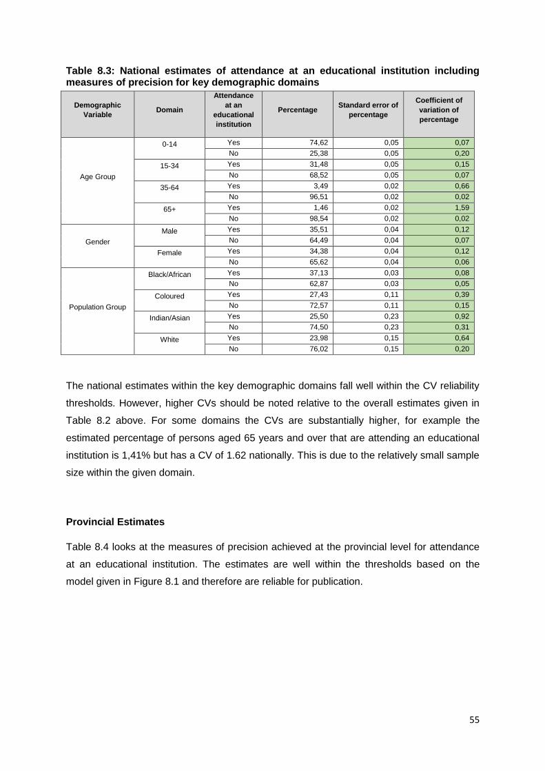
55

Table 8.3: National estimates of attendance at an educational institution including measures of precision for key demographic domains

Demographic

Variable Domain

Attendance

at an

educational

institution

Percentage Standard error of

percentage

Coefficient of

variation of

percentage

Age Group

0-14 Yes 74,62 0,05 0,07

No 25,38 0,05 0,20

15-34 Yes 31,48 0,05 0,15

No 68,52 0,05 0,07

35-64 Yes 3,49 0,02 0,66

No 96,51 0,02 0,02

65+ Yes 1,46 0,02 1,59

No 98,54 0,02 0,02

Gender

Male Yes 35,51 0,04 0,12

No 64,49 0,04 0,07

Female Yes 34,38 0,04 0,12

No 65,62 0,04 0,06

Population Group

Black/African Yes 37,13 0,03 0,08

No 62,87 0,03 0,05

Coloured Yes 27,43 0,11 0,39

No 72,57 0,11 0,15

Indian/Asian Yes 25,50 0,23 0,92

No 74,50 0,23 0,31

White Yes 23,98 0,15 0,64

No 76,02 0,15 0,20

The national estimates within the key demographic domains fall well within the CV reliability

thresholds. However, higher CVs should be noted relative to the overall estimates given in

Table 8.2 above. For some domains the CVs are substantially higher, for example the

estimated percentage of persons aged 65 years and over that are attending an educational

institution is 1,41% but has a CV of 1.62 nationally. This is due to the relatively small sample

size within the given domain.

Provincial Estimates

Table 8.4 looks at the measures of precision achieved at the provincial level for attendance

at an educational institution. The estimates are well within the thresholds based on the

model given in Figure 8.1 and therefore are reliable for publication.

56

Table 8.4: Provincial estimates of attendance at an educational institution including measures of precision

Province

Attendance

at an

educational

institution

Raw

count of

persons

Weighted

count of

persons

Percentage

Standard

error of

percentage

Lower

confidence

limit of

percentage

Upper

confidence

limit of

percentage

Coefficient

of variation

of

percentage

Western

Cape

Yes 75 414 1 765 291 28,16 0,11 27,96 28,37 0,38

No 204 555 4 502 861 71,84 0,11 71,63 72,04 0,15

Eastern

Cape

Yes 171 378 2 833 523 40,53 0,08 40,37 40,69 0,21

No 291 626 4 157 925 59,47 0,08 59,31 59,63 0,14

Northern

Cape

Yes 26 190 358 634 30,07 0,17 29,73 30,41 0,58

No 56 078 833 970 69,93 0,17 69,59 70,27 0,25

Free State Yes 69 263 979 560 34,59 0,12 34,36 34,82 0,34

No 126 149 1 852 431 65,41 0,12 65,18 65,64 0,18

KwaZulu-

Natal

Yes 241 197 4 312 671 39,00 0,07 38,87 39,13 0,17

No 418 101 6 744 689 61,00 0,07 60,87 61,13 0,11

North West Yes 82 410 1 227 737 32,79 0,11 32,58 33,00 0,33

No 165 279 2 516 948 67,21 0,11 67,00 67,42 0,16

Gauteng Yes 216 868 3 911 835 29,27 0,06 29,14 29,39 0,21

No 506 776 9 453 817 70,73 0,06 70,61 70,86 0,09

Mpumalanga Yes 98 688 1 545 593 35,73 0,10 35,52 35,93 0,29

No 171 156 2 780 488 64,27 0,10 64,07 64,48 0,16

Limpopo Yes 171 451 2 476 009 42,76 0,08 42,60 42,92 0,19

No 231 430 3 314 501 57,24 0,08 57,08 57,40 0,14

Total

3 324 009 55 568 486 100,00

Municipal Estimates

If we apply the model as given in Figure 8.1 for the precision estimates of attendance at an

educational institution at municipal level, municipalities can be categorised as given in Table

8.5 below.

57

Table 8.5: Municipalities by CV thresholds for attendance at an educational institution

Province

Attendance

at an

educational

institution

CV Thresholds

CV ≤ 16.5%

(Reliable)

16.6% ≤ CV < 33.4%

(Use with caution)

CV ≥ 33.5%

(Unreliable)

Western Cape

Yes 25 0 0

No 25 0 0

Eastern Cape

Yes 39 0 0

No 39 0 0

Northern

Cape

Yes 27 0 0

No 27 0 0

Free State

Yes 20 0 0

No 20 0 0

KwaZulu-

Natal

Yes 51 0 0

No 51 0 0

North West

Yes 19 0 0

No 19 0 0

Gauteng

Yes 10 0 0

No 10 0 0

Mpumalanga

Yes 18 0 0

No 18 0 0

Limpopo

Yes 25 0 0

No 25 0 0

South Africa

Yes 234 0 0

No 234 0 0

As shown in Table 8.5 above, all municipalities within the country provide sufficiently reliable

estimates for the categories for attendance at an educational institution (see Appendix C for

CVs at municipal level).

58

8.2.1.2. Highest level of education completed

National estimates

Table 8.6 looks at the measures of precision achieved at the national level for highest level

of education completed. The estimates are well within the thresholds based on the model

given in Figure 8.1 and therefore are reliable for publication.

Table 8.6: National estimates of highest level of education completed including measures of precision

Highest level of

education

Raw count

of persons

Weighted

count of

persons

Percentage Standard

Error

Lower

confidence

limit of

percentage

Upper

confidence

limit of

percentage

Coefficient

of variation

of

percentage

No schooling 1 254 640 19 896 975 36,12 0,03 36,06 36,18 0,08

Primary education 1 205 871 19 805 788 35,95 0,03 35,90 36,01 0,08

Secondary education 766 068 13 871 772 25,18 0,03 25,13 25,24 0,11

Bachelor's Degree 60 160 1 336 095 2,43 0,01 2,40 2,45 0,54

Other 9 023 175 597 0,32 0,00 0,31 0,33 1,39

Total 3 295 762 55 086 227 100,00

The national level percentage estimates for highest level of education completed within the

demographic domains of age group, and population group are given in Appendix E. The

national estimates within these key demographic domains generally fall within the CV

reliability thresholds for most of the categories of highest level of education completed.

However, for age group 0–14 the CV achieved for secondary education completed is greater

than 33,5% and therefore is unreliable. This is due to the small number of units realised

within this particular cell.

Provincial estimates

Table 8.7 looks at the measures of precision achieved at the provincial level for highest level

of education completed. The estimates are well within the thresholds based on the model

given in Figure 8.1 and therefore are reliable for publication.

59

Table 8.7: Provincial estimates of highest level of education completed including measures of precision

Province Highest level of

education

Raw

count of

persons

Weighted

count of

persons

Percentage Standard

Error,

Lower

confidence

limit of

percentage

Upper

confidence

limit of

percentage

Coefficient

of

variation

of

percentage

Western Cape

No schooling 82 256 1 829 898 29,64 0,10 29,43 29,85 0,35

Primary education 112 958 2 371 047 38,40 0,11 38,19 38,62 0,29

Secondary education 72 304 1 712 368 27,74 0,11 27,52 27,95 0,39

Bachelor's Degree 7 211 235 798 3,82 0,06 3,70 3,94 1,57

Other 941 24 719 0,40 0,02 0,37 0,43 4,09

Eastern Cape

No schooling 203 769 2 900 305 41,66 0,08 41,50 41,83 0,20

Primary education 182 554 2 808 905 40,35 0,08 40,19 40,51 0,20

Secondary education 67 602 1 135 809 16,32 0,07 16,19 16,45 0,40

Bachelor's Degree 6 131 102 413 1,47 0,02 1,43 1,52 1,59

Other 823 13 629 0,20 0,01 0,18 0,21 4,49

Northern Cape

No schooling 33 740 443 615 37,61 0,18 37,25 37,97 0,49

Primary education 31 270 468 249 39,70 0,19 39,32 40,07 0,48

Secondary education 15 102 246 991 20,94 0,17 20,61 21,27 0,80

Bachelor's Degree 1 035 16 808 1,42 0,05 1,33 1,52 3,48

Other 238 3 936 0,33 0,02 0,29 0,38 7,32

Free State

No schooling 74 470 997 090 35,48 0,12 35,25 35,71 0,33

Primary education 74 136 1 075 901 38,29 0,12 38,05 38,52 0,32

Secondary education 42 000 675 485 24,04 0,11 23,82 24,26 0,47

Bachelor's Degree 2 715 53 095 1,89 0,05 1,80 1,98 2,48

Other 501 8 505 0,30 0,02 0,27 0,33 5,40

KwaZulu-Natal

No schooling 258 883 4 415 503 40,04 0,07 39,92 40,17 0,16

Primary education 226 808 3 683 302 33,40 0,06 33,28 33,52 0,18

Secondary education 160 096 2 726 426 24,73 0,06 24,61 24,84 0,23

Bachelor's Degree 10 354 181 705 1,65 0,02 1,61 1,68 1,08

Other 1 143 19 635 0,18 0,01 0,17 0,19 3,30

North West

No schooling 102 206 1 458 632 39,38 0,11 39,16 39,60 0,28

Primary education 90 235 1 371 447 37,03 0,11 36,81 37,25 0,30

Secondary education 48 566 802 997 21,68 0,10 21,49 21,88 0,46

Bachelor's Degree 3 129 59 090 1,60 0,04 1,52 1,67 2,29

Other 726 11 584 0,31 0,01 0,29 0,34 4,14

Gauteng

No schooling 207 363 3 777 897 28,65 0,06 28,53 28,78 0,22

Primary education 249 405 4 346 773 32,97 0,06 32,84 33,09 0,19

Secondary education 232 987 4 450 618 33,76 0,07 33,62 33,89 0,20

Bachelor's Degree 21 417 549 241 4,17 0,04 4,09 4,24 0,87

Other 2 671 60 242 0,46 0,01 0,43 0,48 2,82

Mpumalanga

No schooling 110 362 1 679 929 39,15 0,11 38,95 39,36 0,27

Primary education 93 296 1 486 674 34,65 0,10 34,45 34,85 0,30

Secondary education 60 786 1 058 713 24,67 0,10 24,48 24,87 0,40

Bachelor's Degree 2 521 52 575 1,23 0,03 1,16 1,29 2,81

Other 723 12 937 0,30 0,01 0,28 0,33 4,29

Limpopo

No schooling 181 591 2 394 106 41,60 0,08 41,43 41,76 0,20

Primary education 145 209 2 193 490 38,11 0,08 37,95 38,27 0,22

Secondary education 66 625 1 062 366 18,46 0,07 18,32 18,59 0,37

Bachelor's Degree 5 647 85 370 1,48 0,02 1,44 1,53 1,45

Other 1 257 20 410 0,35 0,01 0,33 0,38 3,02

Total 3 295 762 55 086 227 100,00

60

Municipal estimates

If we apply the model as given in Figure 8.1 for the precision estimates highest level of

education completed at municipal level, municipalities can be categorised as given in Table

8.8 below.

Table 8.8: Municipalities by CV thresholds for highest level of education completed

Province Highest level of

education

CV Thresholds

CV ≤ 16.5%

(Reliable)

16.6% ≤ CV < 33.4%

(Use with caution)

CV ≥ 33.5%

(Unreliable)

Western Cape

No schooling 25 0 0

Primary education 25 0 0

Secondary education 25 0 0

Bachelor's Degree 16 6 3

Other 1 11 12

Eastern Cape

No schooling 39 0 0

Primary education 39 0 0

Secondary education 39 0 0

Bachelor's Degree 24 12 3

Other 3 18 16

Northern Cape

No schooling 27 0 0

Primary education 27 0 0

Secondary education 27 0 0

Bachelor's Degree 4 14 9

Other 2 5 17

Free State

No schooling 20 0 0

Primary education 20 0 0

Secondary education 20 0 0

Bachelor's Degree 13 6 1

Other 4 9 6

KwaZulu-Natal

No schooling 51 0 0

Primary education 51 0 0

Secondary education 51 0 0

Bachelor's Degree 30 21 0

Other 4 18 27

North West

No schooling 19 0 0

Primary education 19 0 0

Secondary education 19 0 0

Bachelor's Degree 13 6 0

Other 6 10 3

Gauteng

No schooling 10 0 0

Primary education 10 0 0

Secondary education 10 0 0

Bachelor's Degree 9 1 0

Other 6 4 0

Mpumalanga No schooling 18 0 0

61

Province Highest level of

education

CV Thresholds

CV ≤ 16.5%

(Reliable)

16.6% ≤ CV < 33.4%

(Use with caution)

CV ≥ 33.5%

(Unreliable)

Primary education 18 0 0

Secondary education 18 0 0

Bachelor's Degree 13 5 0

Other 7 5 6

Limpopo

No schooling 25 0 0

Primary education 25 0 0

Secondary education 25 0 0

Bachelor's Degree 24 1 0

Other 12 10 2

South Africa

No schooling 234 0 0

Primary education 234 0 0

Secondary education 234 0 0

Bachelor's Degree 146 72 16

Other 45 90 89

As shown in Table 8.8 above, most municipalities within the country provide sufficiently

reliable estimates for the categories for highest level of education completed. However, there

are some categories (i.e. Bachelor’s degree and Other) for some municipalities where the

estimates are less reliable and cautioned should be exercised due to the small cell sizes

(see Appendix D for CVs at municipal level).

8.2.2. Household level indicators

This section analyses the CVs at national, provincial and municipal levels obtained for the

following key indicators at household level:

Type of main dwelling

Water source

8.2.2.1. Type of main dwelling

National and provincial estimates

Table 8.9 looks at the measures of precision achieved at both national and provincial levels

for the type of main dwelling. The national and provincial estimates for this variable are well

within the thresholds based on the model given in Figure 8.1 and therefore are reliable.

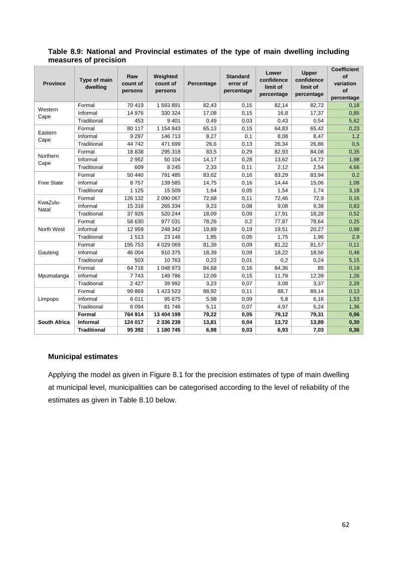
62

Table 8.9: National and Provincial estimates of the type of main dwelling including measures of precision

Province Type of main

dwelling

Raw

count of

persons

Weighted

count of

persons

Percentage

Standard

error of

percentage

Lower

confidence

limit of

percentage

Upper

confidence

limit of

percentage

Coefficient

of

variation

of

percentage

Western

Cape

Formal 70 419 1 593 891 82,43 0,15 82,14 82,72 0,18

Informal 14 976 330 324 17,08 0,15 16,8 17,37 0,85

Traditional 453 9 401 0,49 0,03 0,43 0,54 5,62

Eastern

Cape

Formal 80 117 1 154 843 65,13 0,15 64,83 65,42 0,23

Informal 9 297 146 713 8,27 0,1 8,08 8,47 1,2

Traditional 44 742 471 699 26,6 0,13 26,34 26,86 0,5

Northern

Cape

Formal 18 838 295 318 83,5 0,29 82,93 84,08 0,35

Informal 2 952 50 104 14,17 0,28 13,62 14,72 1,98

Traditional 609 8 245 2,33 0,11 2,12 2,54 4,66

Free State

Formal 50 440 791 485 83,62 0,16 83,29 83,94 0,2

Informal 8 757 139 585 14,75 0,16 14,44 15,06 1,08

Traditional 1 125 15 509 1,64 0,05 1,54 1,74 3,18

KwaZulu-

Natal

Formal 126 132 2 090 067 72,68 0,11 72,46 72,9 0,16

Informal 15 318 265 334 9,23 0,08 9,08 9,38 0,83

Traditional 37 926 520 244 18,09 0,09 17,91 18,28 0,52

North West

Formal 58 630 977 031 78,26 0,2 77,87 78,64 0,25

Informal 12 959 248 342 19,89 0,19 19,51 20,27 0,98

Traditional 1 513 23 146 1,85 0,05 1,75 1,96 2,9

Gauteng

Formal 195 753 4 029 069 81,39 0,09 81,22 81,57 0,11

Informal 46 004 910 375 18,39 0,09 18,22 18,56 0,48

Traditional 503 10 763 0,22 0,01 0,2 0,24 5,15

Mpumalanga

Formal 64 716 1 048 973 84,68 0,16 84,36 85 0,19

Informal 7 743 149 786 12,09 0,15 11,79 12,39 1,26

Traditional 2 427 39 992 3,23 0,07 3,08 3,37 2,28

Limpopo

Formal 99 869 1 423 523 88,92 0,11 88,7 89,14 0,13

Informal 6 011 95 675 5,98 0,09 5,8 6,16 1,53

Traditional 6 094 81 746 5,11 0,07 4,97 5,24 1,36

South Africa

Formal 764 914 13 404 199 79,22 0,05 79,12 79,31 0,06

Informal 124 017 2 336 239 13,81 0,04 13,72 13,89 0,30

Traditional 95 392 1 180 745 6,98 0,03 6,93 7,03 0,36

Municipal estimates

Applying the model as given in Figure 8.1 for the precision estimates of type of main dwelling

at municipal level, municipalities can be categorised according to the level of reliability of the

estimates as given in Table 8.10 below.

63

Table 8.10: Municipalities by CV thresholds for type of main dwelling

Province Type of main

dwelling

CV Thresholds

CV ≤ 16.5%

(Reliable)

16.6% ≤ CV < 33.4%

(Use with caution)

CV ≥ 33.5%

(Unreliable)

Western Cape

Formal 25 0 0

Informal 18 3 4

Traditional 2 11 10

Eastern Cape

Formal 39 0 0

Informal 26 10 2

Traditional 24 7 4

Northern Cape

Formal 27 0 0

Informal 15 8 4

Traditional 3 3 14

Free State

Formal 20 0 0

Informal 20 0 0

Traditional 4 6 9

KwaZulu-Natal

Formal 51 0 0

Informal 33 12 5

Traditional 51 0 0

North West

Formal 19 0 0

Informal 19 0 0

Traditional 9 4 6

Gauteng

Formal 10 0 0

Informal 10 0 0

Traditional 3 2 5

Mpumalanga

Formal 18 0 0

Informal 18 0 0

Traditional 14 2 2

Limpopo

Formal 25 0 0

Informal 23 2 0

Traditional 17 3 5

South Africa

Formal 234 0 0

Informal 182 35 15

Traditional 127 38 55

64

The majority of the municipalities across provinces have reliable estimates in the three

categories of type of main dwelling. There are municipalities distributed across provinces

with estimates for informal and traditional main dwelling types (i.e. 35 and 38 municipalities

respectively) that have higher CVs and these estimates should be used with caution.

Furthermore, there are 15 municipalities who have survey estimates that are unreliable for

informal dwelling types and 55 municipalities that are unreliable for traditional dwelling types.

See Table 8.11 for the list of such municipalities.

Table 8.11: Municipalities with unreliable estimates for type of main dwelling

Province Municipality Type of main

dwelling Weighted count of Households

Percentage Coefficient of variation of percentage

Western Cape

Beaufort West Informal 66 0,44 45,84

Kannaland Informal 162 2,57 38,00

Laingsburg Informal 47 1,62 70,26

Prince Albert Informal 8 0,19 100,45

Bitou Traditional 202 0,92 57,15

Cederberg Traditional 140 0,91 43,01

Drakenstein Traditional 151 0,21 42,83

George Traditional 498 0,79 37,31

Knysna Traditional 82 0,32 41,41

Laingsburg Traditional 24 0,85 99,78

Matzikama Traditional 81 0,39 50,07

Oudtshoorn Traditional 50 0,21 53,28

Stellenbosch Traditional 366 0,70 47,43

Swellendam Traditional 24 0,20 100,02

Eastern Cape

Baviaans Informal 101 2,18 39,91

Inkwanca Informal 169 2,78 38,36

Baviaans Traditional 96 2,07 44,99

Camdeboo Traditional 47 0,36 72,48

Inkwanca Traditional 119 1,97 46,55

Inxuba Yethemba Traditional 28 0,15 75,40

Northern Cape

Kamiesberg Informal 121 3,63 36,08

Kareeberg Informal 131 3,56 51,38

Karoo Hoogland Informal 25 0,55 79,78

Richtersveld Informal 53 1,25 52,69

Dikgatlong Traditional 117 0,79 38,55

Kareeberg Traditional 81 2,21 56,26

Kgatelopele Traditional 19 0,31 99,96

Khâi-Ma Traditional 41 0,99 70,57

Magareng Traditional 15 0,22 100,05

Mier Traditional 27 1,32 99,37

Phokwane Traditional 33 0,17 63,18

Richtersveld Traditional 2 0,05 100,38

Siyancuma Traditional 17 0,17 79,91

Sol Plaatjie Traditional 129 0,18 36,58

Thembelihle Traditional 61 1,30 71,69

Tsantsabane Traditional 36 0,30 79,02

Ubuntu Traditional 11 0,18 100,18

Umsobomvu Traditional 15 0,15 100,06

Free State

Kopanong Traditional 43 0,23 79,77

Letsemeng Traditional 10 0,07 100,08

Masilonyana Traditional 48 0,21 61,75

Metsimaholo Traditional 46 0,08 71,84

Mohokare Traditional 13 0,11 100,03

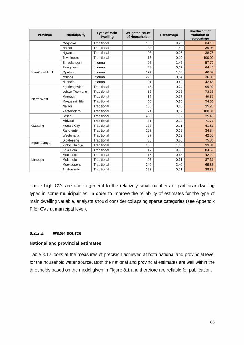
65

Province Municipality Type of main

dwelling Weighted count of Households

Percentage Coefficient of variation of percentage

Moqhaka Traditional 108 0,20 34,15

Naledi Traditional 133 1,59 39,08

Ngwathe Traditional 108 0,26 38,75

Tswelopele Traditional 13 0,10 100,00

KwaZulu-Natal

Emadlangeni Informal 97 1,45 57,72

Ezingoleni Informal 29 0,27 64,40

Mpofana Informal 174 1,50 46,37

Msinga Informal 220 0,54 36,05

Nkandla Informal 91 0,42 42,45

North West

Kgetlengrivier Traditional 45 0,24 99,92

Lekwa-Teemane Traditional 63 0,38 73,38

Mamusa Traditional 57 0,37 49,51

Maquassi Hills Traditional 68 0,28 54,83

Naledi Traditional 130 0,63 35,20

Ventersdorp Traditional 21 0,12 100,01

Gauteng

Lesedi Traditional 438 1,12 35,48

Midvaal Traditional 51 0,13 71,71

Mogale City Traditional 165 0,11 41,81

Randfontein Traditional 163 0,29 34,84

Westonaria Traditional 87 0,19 42,55

Mpumalanga Dipaleseng Traditional 30 0,20 75,36

Victor Khanye Traditional 288 1,18 33,81

Limpopo

Bela-Bela Traditional 17 0,08 84,52

Modimolle Traditional 116 0,63 42,22

Molemole Traditional 93 0,31 37,31

Mookgopong Traditional 249 2,40 69,83

Thabazimbi Traditional 253 0,71 38,88

These high CVs are due in general to the relatively small numbers of particular dwelling

types in some municipalities. In order to improve the reliability of estimates for the type of

main dwelling variable, analysts should consider collapsing sparse categories (see Appendix

F for CVs at municipal level).

8.2.2.2. Water source

National and provincial estimates

Table 8.12 looks at the measures of precision achieved at both national and provincial level

for the household water source. Both the national and provincial estimates are well within the

thresholds based on the model given in Figure 8.1 and therefore are reliable for publication.

66

Table 8.12: National and provincial estimates of the type of main dwelling including measures of precision

Province Water source

Raw

count of

persons

Weighted

count of

persons

Percentage

Standard

error of

percentage

Coefficient

of

variation

of

percentage

Western

Cape

Piped water inside dwelling 64 896 1 487 774 76,93 0,16 0,21

Piped water inside yard 11 485 232 892 12,04 0,12 1,01

Piped water from access point outside the yard 9 085 204 414 10,57 0,12 1,12

No access to piped water 394 8 797 0,45 0,03 5,99

Eastern

Cape

Piped water inside dwelling 35 324 592 428 33,41 0,17 0,49

Piped water inside yard 32 650 433 028 24,42 0,14 0,56

Piped water from access point outside the yard 35 726 429 037 24,19 0,13 0,55

No access to piped water 30 466 318 902 17,98 0,11 0,63

Northern

Cape

Piped water inside dwelling 9 429 154 529 43,69 0,38 0,88

Piped water inside yard 8 047 129 197 36,53 0,37 1,02

Piped water from access point outside the yard 4 585 64 272 18,17 0,29 1,58

No access to piped water 340 5 710 1,61 0,14 8,83

Free State

Piped water inside dwelling 20 957 357 926 37,81 0,23 0,61

Piped water inside yard 35 101 519 086 54,83 0,23 0,42

Piped water from access point outside the yard 3 776 62 136 6,56 0,12 1,76

No access to piped water 491 7 490 0,79 0,04 4,99

KwaZulu-

Natal

Piped water inside dwelling 61 544 1 076 667 37,44 0,13 0,34

Piped water inside yard 61 430 965 066 33,56 0,12 0,36

Piped water from access point outside the yard 39 772 616 299 21,43 0,11 0,49

No access to piped water 16 642 217 811 7,57 0,06 0,85

North West

Piped water inside dwelling 15 739 300 221 24,04 0,20 0,82

Piped water inside yard 36 340 616 426 49,36 0,22 0,45

Piped water from access point outside the yard 19 897 310 170 24,84 0,18 0,72

No access to piped water 1 140 21 950 1,76 0,06 3,56

Gauteng

Piped water inside dwelling 140 404 2 972 973 60,05 0,11 0,19

Piped water inside yard 81 372 1 568 039 31,67 0,11 0,34

Piped water from access point outside the yard 19 885 396 334 8,00 0,06 0,79

No access to piped water 647 13 792 0,28 0,02 5,40

Mpumalanga

Piped water inside dwelling 18 238 359 033 28,98 0,21 0,73

Piped water inside yard 40 937 630 078 50,86 0,21 0,42

Piped water from access point outside the yard 12 960 207 087 16,72 0,15 0,92

No access to piped water 2 758 42 663 3,44 0,08 2,24

Limpopo

Piped water inside dwelling 13 216 210 302 13,14 0,12 0,91

Piped water inside yard 50 589 721 579 45,07 0,16 0,36

Piped water from access point outside the yard 40 230 562 950 35,16 0,16 0,45

No access to piped water 7 951 106 251 6,64 0,08 1,19

South Africa

Piped water inside dwelling 379 747 7 511 853 44,39 0,06 0,14

Piped water inside yard 357 951 5 815 391 34,36 0,05 0,16

Piped water from access point outside the yard 185 916 2 852 700 16,86 0,04 0,25

No access to piped water 60 829 743 366 4,39 0,02 0,47

Municipal estimates

Applying the model as given in Figure 8.1 for the precision estimates of water source at

municipal level, municipalities can be categorised according to the level of reliability of the

estimates produced as given in Table 8.13 below.

67

Table 8.13: Municipalities by CV thresholds for water source

Province Water source

CV Thresholds

CV ≤ 16.5%

(Reliable)

16.6% ≤ CV < 33.4%

(Use with caution)

CV ≥ 33.5%

(Unreliable)

Western Cape

Piped water inside dwelling 25 0 0

Piped water inside yard 24 1 0

Piped water from access point outside the yard 15 6 4

No access to piped water 1 13 11

Eastern Cape

Piped water inside dwelling 35 4 0

Piped water inside yard 38 1 0

Piped water from access point outside the yard 30 6 3

No access to piped water 22 5 11

Northern Cape

Piped water inside dwelling 27 0 0

Piped water inside yard 27 0 0

Piped water from access point outside the yard 10 12 5

No access to piped water 1 5 18

Free State

Piped water inside dwelling 20 0 0

Piped water inside yard 20 0 0

Piped water from access point outside the yard 16 4 0

No access to piped water 2 7 9

KwaZulu-Natal

Piped water inside dwelling 41 10 0

Piped water inside yard 51 0 0

Piped water from access point outside the yard 49 2 0

No access to piped water 43 6 2

North West

Piped water inside dwelling 18 1 0

Piped water inside yard 19 0 0

Piped water from access point outside the yard 17 2 0

No access to piped water 7 6 6

Gauteng

Piped water inside dwelling 10 0 0

Piped water inside yard 10 0 0

Piped water from access point outside the yard 10 0 0

No access to piped water 3 4 3

Mpumalanga

Piped water inside dwelling 18 0 0

Piped water inside yard 18 0 0

Piped water from access point outside the yard 18 0 0

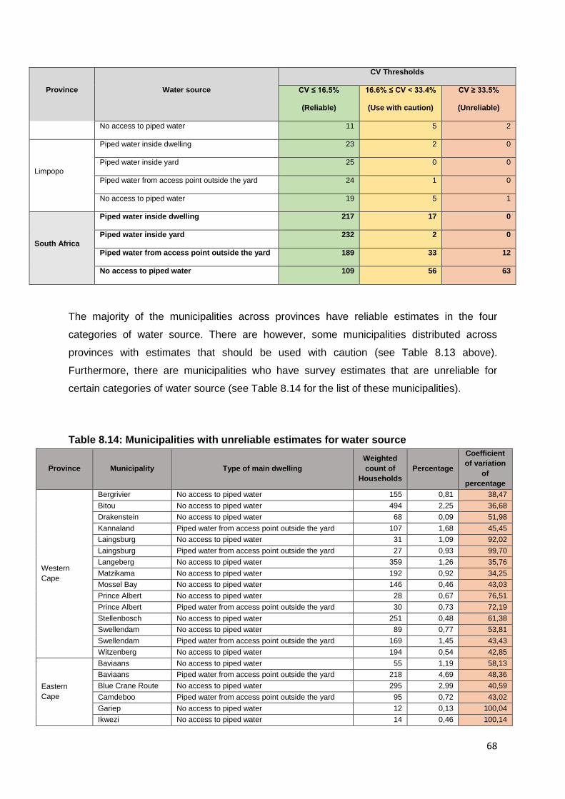
68

Province Water source

CV Thresholds

CV ≤ 16.5%

(Reliable)

16.6% ≤ CV < 33.4%

(Use with caution)

CV ≥ 33.5%

(Unreliable)

No access to piped water 11 5 2

Limpopo

Piped water inside dwelling 23 2 0

Piped water inside yard 25 0 0

Piped water from access point outside the yard 24 1 0

No access to piped water 19 5 1

South Africa

Piped water inside dwelling 217 17 0

Piped water inside yard 232 2 0

Piped water from access point outside the yard 189 33 12

No access to piped water 109 56 63

The majority of the municipalities across provinces have reliable estimates in the four

categories of water source. There are however, some municipalities distributed across

provinces with estimates that should be used with caution (see Table 8.13 above).

Furthermore, there are municipalities who have survey estimates that are unreliable for

certain categories of water source (see Table 8.14 for the list of these municipalities).

Table 8.14: Municipalities with unreliable estimates for water source

Province Municipality Type of main dwelling

Weighted

count of

Households

Percentage

Coefficient

of variation

of

percentage

Western

Cape

Bergrivier No access to piped water 155 0,81 38,47

Bitou No access to piped water 494 2,25 36,68

Drakenstein No access to piped water 68 0,09 51,98

Kannaland Piped water from access point outside the yard 107 1,68 45,45

Laingsburg No access to piped water 31 1,09 92,02

Laingsburg Piped water from access point outside the yard 27 0,93 99,70

Langeberg No access to piped water 359 1,26 35,76

Matzikama No access to piped water 192 0,92 34,25

Mossel Bay No access to piped water 146 0,46 43,03

Prince Albert No access to piped water 28 0,67 76,51

Prince Albert Piped water from access point outside the yard 30 0,73 72,19

Stellenbosch No access to piped water 251 0,48 61,38

Swellendam No access to piped water 89 0,77 53,81

Swellendam Piped water from access point outside the yard 169 1,45 43,43

Witzenberg No access to piped water 194 0,54 42,85

Eastern

Cape

Baviaans No access to piped water 55 1,19 58,13

Baviaans Piped water from access point outside the yard 218 4,69 48,36

Blue Crane Route No access to piped water 295 2,99 40,59

Camdeboo Piped water from access point outside the yard 95 0,72 43,02

Gariep No access to piped water 12 0,13 100,04

Ikwezi No access to piped water 14 0,46 100,14

69

Province Municipality Type of main dwelling

Weighted

count of

Households

Percentage

Coefficient

of variation

of

percentage

Ikwezi Piped water from access point outside the yard 102 3,44 69,85

Inkwanca No access to piped water 40 0,66 99,61

Inxuba Yethemba No access to piped water 120 0,66 45,22

Kouga No access to piped water 61 0,17 54,37

Makana No access to piped water 587 2,59 33,69

Maletswai No access to piped water 50 0,36 55,59

Nxuba No access to piped water 48 0,75 64,18

Tsolwana No access to piped water 36 0,40 56,51

Northern

Cape

!Kheis No access to piped water 119 2,73 42,92

//Khara Hais No access to piped water 171 0,64 39,95

Dikgatlong No access to piped water 177 1,20 33,65

Emthanjeni No access to piped water 12 0,10 43,79

Gamagara No access to piped water 122 0,77 51,20

Hantam No access to piped water 56 0,82 71,85

Kamiesberg No access to piped water 40 1,21 70,88

Kamiesberg Piped water from access point outside the yard 94 2,84 60,18

Kareeberg No access to piped water 58 1,57 70,81

Kareeberg Piped water from access point outside the yard 228 6,20 40,18

Karoo Hoogland Piped water from access point outside the yard 81 1,74 46,88

Khâi-Ma No access to piped water 96 2,33 52,19

Khâi-Ma Piped water from access point outside the yard 66 1,62 64,54

Magareng No access to piped water 64 0,92 58,97

Mier No access to piped water 62 3,06 57,14

Nama Khoi No access to piped water 142 0,97 46,38

Renosterberg No access to piped water 28 0,79 99,73

Renosterberg Piped water from access point outside the yard 154 4,31 34,88

Richtersveld No access to piped water 96 2,29 41,18

Sol Plaatjie No access to piped water 303 0,42 49,16

Thembelihle No access to piped water 79 1,67 59,21

Ubuntu No access to piped water 14 0,23 100,12

Umsobomvu No access to piped water 4 0,04 100,18

Free State

Kopanong No access to piped water 90 0,49 43,61

Letsemeng No access to piped water 65 0,46 61,44

Mafube No access to piped water 85 0,45 48,57

Mantsopa No access to piped water 83 0,49 42,84

Metsimaholo No access to piped water 67 0,11 51,30

Mohokare No access to piped water 35 0,28 70,88

Moqhaka No access to piped water 223 0,42 35,70

Naledi No access to piped water 32 0,38 70,66

Tswelopele No access to piped water 191 1,40 33,93

KwaZulu-

Natal

Umdoni No access to piped water 100 0,38 44,00

uMhlathuze No access to piped water 117 0,11 38,29

North West

Kgetlengrivier No access to piped water 131 0,70 35,98

Lekwa-Teemane No access to piped water 43 0,26 58,24

Mamusa No access to piped water 87 0,56 38,83

Maquassi Hills No access to piped water 104 0,43 46,42

Naledi No access to piped water 113 0,55 41,67

Ventersdorp No access to piped water 183 1,07 36,72

Gauteng

Lesedi No access to piped water 214 0,55 36,58

Midvaal No access to piped water 60 0,16 58,82

Mogale City No access to piped water 614 0,42 40,12

Mpumalanga Dipaleseng No access to piped water 70 0,47 48,44

Lekwa No access to piped water 148 0,40 36,42

Limpopo Bela-Bela No access to piped water 307 1,44 40,90

70

From Table 8.14 above, categories of water source with relatively smaller sample sizes in

these municipalities have high CVs and therefore the estimates are unreliable. In order to

improve the reliability of estimates for the type of main dwelling variable, analysts should

consider collapsing sparse categories (see Appendix G for CVs at municipal level).

8.3. Note on analysis of domains

The analysis given in the sections above show that survey estimates for all categories of the

key variables at national and provincial level are reliable. At municipal level, however there

are some categories where caution needs to be exercised when interpreting the survey

estimates, due to the relatively small number of units within these cells (see Table 8.11 and

8.14 above). In addition, when cross tabulating these variables with other analysis variables

for analysing particular domains the cell sizes will be further reduced. This effect will be

greater at local municipality level and therefore analysts are cautioned that any analysis of

particular domains especially at local municipality level need to have adequate sample sizes

within each cell in order to obtain reliable survey estimates. If cell sizes are too small,

analysts should try to collapse some cells to increase the cell sizes.

71

9. Appendices

Appendix A: Response Rates at Local Municipality Level

Appendix B: Out-of-Scope Rates at Local Municipality Level

Appendix C: Precision Estimates at Local Municipality Level for Educational Attendance

Appendix D:

Precision Estimates for Highest Level of Education by Key Demographic Variables

Nationally

Appendix E: Precision Estimates at Local Municipality Level for Highest level of Education

Appendix F: Precision Estimates at Local Municipality Level for Main Dwelling Type

Appendix G: Precision Estimates at Local Municipality Level for Main Source of Water

NB: All appendices are available on the CS 2016 webpage. If you are using an

electronic version of this report, please click here to access the appendices.

72

10. References

1) Project Charter, Community Survey 2016. Statistics South Africa.

2) Data Collection Methodology, Community Survey 2016. Statistics South Africa.

3) The Hard-to-Count Population Strategy, Community Survey 2016. Statistics South Africa.

4) Field Training Plan, Community Survey 2016. Statistics South Africa.

5) Weighting Strategy, Community Survey 2016. Statistics South Africa.

6) Weighting Accountability Report, Community Survey 2016. Statistics South Africa.

7) Dwelling Units Sampling Report, Community Survey 2016. Statistics South Africa.

8) Standard on Calculation of Response Rates for Household Surveys. December 2011.

Statistics South Africa.

9) Standard on Classification of Result Codes for Enumeration of Households. March 2016.

Statistics South Africa.