commercial motor vehicle driver restart study: final report driver restart...naturalistic study of...

Commercial Motor Vehicle (CMV) Driver Restart Study: Final Report

December 2015

FOREWORD The Federal Motor Carrier Safety Administration (FMCSA) awarded a contract to conduct a naturalistic study of the operational, safety, health, and fatigue impacts of the two restart provisions (i.e., the requirement for two nighttime periods [1–5 a.m.] during a 34-hour restart, and the requirement for a minimum of 168 hours between the beginning of a 34-hour restart period and the beginning of the previous 34-hour restart period—see Sections 395.3(c) and 395.3(d) of Title 49, Code of Federal Regulations) on commercial motor vehicle (CMV) drivers. This naturalistic study included a sample of drivers large enough to produce statistically significant results. The study compared the effects of different recovery times using both an in-subject and between-subject research design. It was expected that the two groups of drivers operating under the two restart conditions would overlap, and consequently a paired study design was used to take advantage of its statistical power. This report documents the methods, data analyses, results, and conclusions involved in successfully conducting this study and evaluating the data.

NOTICE This document is disseminated under the sponsorship of the U.S. Department of Transportation (USDOT) in the interest of information exchange. The U.S. Government assumes no liability for the use of the information contained in this document. The contents of this report reflect the views of the contractor, who is responsible for the accuracy of the data presented herein. The contents do not necessarily reflect the official policy of the USDOT. This report does not constitute a standard, specification, or regulation.

The U.S. Government does not endorse products or manufacturers named herein. Trademarks or manufacturers’ names appear in this report only because they are considered essential to the objective of this report.

QUALITY ASSURANCE STATEMENT FMCSA provides high-quality information to serve the Government, industry, and the public in a manner that promotes public understanding. Standards and policies are used to ensure and maximize the quality, objectivity, utility, and integrity of its information. FMCSA periodically reviews quality issues and adjusts its programs and processes to ensure continuous quality improvement.

i

Technical Report Documentation Page 1. Report No. FMCSA-RRR-15-011

2. Government Accession No.

3. Recipient's Catalog No.

4. Title and Subtitle Commercial Motor Vehicle (CMV) Driver Restart Study: Final Report

5. Report Date December 2015 6. Performing Organization Code

7. Author(s) Dinges, David F.; Maislin, Greg; Hanowski, Richard J.; Mollicone, Daniel J.; Hickman, Jeffrey S.; Maislin, David; Kan, Kevin; Hammond, Rebecca L.; Soccolich, Susan A.; Moeller, Devon D., Trentalange, Michael

8. Performing Organization Report No.

9. Performing Organization Name and Address Virginia Tech Transportation Institute 3500 Transportation Research Plaza, Blacksburg, VA 24061 Perelman School of Medicine, University of Pennsylvania Biomedical Statistical Consulting Pulsar Informatics, Inc. Lytx, Inc.

10. Work Unit No. (TRAIS) 11. Contract or Grant No. DTMC75-14-D-00011, Task Order#9

12. Sponsoring Agency Name and Address U.S. Department of Transportation Federal Motor Carrier Safety Administration Office of Analysis, Research, and Technology 1200 New Jersey Ave. SE Washington, DC 20590

13. Type of Report and Period Covered Final Report, December 2014–December 2015

14. Sponsoring Agency Code FMCSA

15. Supplementary Notes Contracting Officer’s Representative: Martin Walker 16. Abstract A congressionally-mandated naturalistic study was conducted to evaluate the operational, safety, fatigue, and health impacts of the restart provisions in Sections 395.3(c) and 395.3(d) of Title 49, Code of Federal Regulations. A total of 235 commercial motor vehicle drivers representative of the industry contributed data while working their normal schedules, with 181 drivers completing all 5 months of the study. Drivers were monitored via electronic logging devices to track driving and working hours; onboard monitoring systems to detect safety-critical events; wrist actigraph devices for sleep-wake tracking; and smartphone apps for self-ratings of fatigue, sleepiness, stress, sleep quality, and caffeine intake, as well as Brief Psychomotor Vigilance Test (PVT-B) performance testing. Drivers provided 26,964 days of data (17,628 duty days and 9,336 restart days). A total of 3,287 restart/duty cycle sampling units were analyzed. Statistical comparisons were performed using linear and non-linear mixed-effects modeling designed to ensure results were free of selection bias. An analysis of the safety-critical event data did not identify any differences in performance. Drivers’ fatigue ratings were higher, and sleep quality ratings were lower, during 1-night versus 2-night restarts [Section 395.3(c)]. Drivers averaged slower PVT-B response times and more PVT-B lapses during restarts after 168 hours than prior to 168 hours [Section 395.3(d)]. During restarts, drivers obtained significantly more sleep (on average, 2 hours more per day), and rated their sleep quality higher and their stress lower as compared to duty days, regardless of provision use. Results indicate that restarts serve to mitigate driver fatigue, stress, and sleep loss (i.e., the restart effectively provides the functional equivalent of a “week end” to recover from fatigue and sleep loss). 17. Key Words Commercial motor vehicle, CMV Driver Restart Study, Consolidated and Further Continuing Appropriations Act of 2015, crash, fatigue, drowsiness, hours-of-service

18. Distribution Statement No restrictions

19. Security Classif. (of this report) Unclassified

20. Security Classif. (of this page) Unclassified

21. No. of Pages 188

22. Price

Form DOT F 1700.7 (8-72) Reproduction of completed page authorized.

ii

SI* (MODERN METRIC) CONVERSION FACTORS Approximate Conversions to SI Units

Symbol When You Know Multiply By To Find Symbol Length

in ft yd mi

inches feet yards miles

25.4 0.305 0.914 1.61

millimeters meters meters kilometers

mm m m km

Area in² ft² yd² ac mi²

square inches square feet square yards Acres square miles

645.2 0.093 0.836 0.405 2.59

square millimeters square meters square meters hectares square kilometers

mm² m² m² ha km²

Volume (volumes greater than 1,000L shall be shown in m³) fl oz gal ft³ yd³

fluid ounces gallons cubic feet cubic yards

29.57 3.785 0.028 0.765

milliliters liters cubic meters cubic meters

mL L m³ m³

Mass oz lb T

ounces pounds short tons (2,000 lb)

28.35 0.454 0.907

grams kilograms megagrams (or “metric ton”)

g kg Mg (or “t”)

Temperature (exact degrees) °F Fahrenheit 5(F-32)/9 or (F-32)/1.8 Celsius °C

Illumination fc fl

foot-candles foot-Lamberts

10.76 3.426

lux candela/m²

lx cd/m²

Force and Pressure or Stress lbf lbf/in²

poundforce poundforce per square inch

4.45 6.89

newtons kilopascals

N kPa

Approximate Conversions from SI Units Symbol When You Know Multiply By To Find Symbol

Length mm m m km

millimeters meters meters kilometers

0.039 3.28 1.09

0.621

inches feet yards miles

in ft yd mi

Area mm² m² m² Ha km²

square millimeters square meters square meters hectares square kilometers

0.0016 10.764 1.195 2.47

0.386

square inches square feet square yards acres square miles

in² ft² yd² ac mi²

Volume mL L m³ m³

milliliters liters cubic meters cubic meters

0.034 0.264 35.314 1.307

fluid ounces gallons cubic feet cubic yards

fl oz gal ft³ yd³

Mass g kg Mg (or “t”)

grams kilograms megagrams (or “metric ton”)

0.035 2.202 1.103

ounces pounds short tons (2,000 lb)

oz lb T

Temperature (exact degrees) °C Celsius 1.8c+32 Fahrenheit °F

Illumination lx cd/m²

lux candela/m²

0.0929 0.2919

foot-candles foot-Lamberts

fc fl

Force and Pressure or Stress N kPa

newtons kilopascals

0.225 0.145

poundforce poundforce per square inch

lbf lbf/in²

* SI is the symbol for the International System of Units. Appropriate rounding should be made to comply with Section 4 of ASTM E380. (Revised March 2003, Section 508-accessible version September 2009.)

iii

TABLE OF CONTENTS

EXECUTIVE SUMMARY .........................................................................................................xv

1. INTRODUCTION.................................................................................................................1

1.1 LITERATURE REVIEW SUMMARY .........................................................................1

1.2 PROJECT SUMMARY .................................................................................................2

1.3 RESEARCH OBJECTIVES ..........................................................................................6

1.4 OPERATIONAL IMPACTS .........................................................................................6 1.4.1 Safety Impacts ................................................................................................... 7 1.4.2 Fatigue Impacts ................................................................................................. 7 1.4.3 Health Impacts .................................................................................................. 7

2. ASSESSMENT TECHNOLOGIES ....................................................................................9

2.1 ONBOARD MONITORING SYSTEMS ERROR! BOOKMARK NOT DEFINED. 2.1.1 Overview of DriveCam Program .................................................................... 10 2.1.2 Issues Encountered with the Onboard Monitoring Systems ........................... 12

2.2 ELECTRONIC LOGGING DEVICES.... ERROR! BOOKMARK NOT DEFINED. 2.2.1 Issues Encountered with Electronic Logging Devices.................................... 13

2.3 ACTIGRAPHY ........................................ ERROR! BOOKMARK NOT DEFINED. 2.3.1 Issues Encountered with Actigraphy Devices................................................. 14

2.4 SMARTPHONE APPS ................................................................................................14 2.4.1 Custom Smartphone Data Collection App ...................................................... 14 2.4.2 Issues Encountered with Smartphone-based Measures .................................. 17 2.4.3 Preexisting Health/Medical Conditions .......................................................... 18

3. METHODS AND APPROACH .........................................................................................19

3.1 OVERVIEW ................................................................................................................19

3.2 INSTITUTIONAL REVIEW BOARD.... ERROR! BOOKMARK NOT DEFINED. 3.3 RECRUITMENT ..................................... ERROR! BOOKMARK NOT DEFINED.

3.3.1 Sampling Plan ................................................................................................. 19 3.3.2 Industry Outreach............................................................................................ 21 3.3.3 Carrier Participation ........................................................................................ 21 3.3.4 Web-based Screening and Enrollment of Drivers .......................................... 22 3.3.5 Empanelment Logistics ................................................................................... 22

3.4 DRIVER RETENTION ...............................................................................................23

3.5 PARTICIPANT BRIEFING ........................................................................................24 3.5.1 Pre-study Briefing ........................................................................................... 24

iv

3.5.2 Weekly Debriefs ............................................................................................. 24 3.5.3 Final Debriefing .............................................................................................. 25

3.6 VEHICLE INSTALLATION ......................................................................................25

3.7 DATA COLLECTION ................................................................................................25 3.7.1 Onboard Monitoring System Data .................................................................. 25 3.7.2 Smartphone App Data ..................................................................................... 29 3.7.3 Electronic Logging Device Data ..................................................................... 30 3.7.4 Actigraph Data ................................................................................................ 30

3.8 METHODOLOGY LIMITATIONS ........ ERROR! BOOKMARK NOT DEFINED.

4. ANALYSIS PLAN AND DATA PROCESSING .............................................................33

4.1 CONCEPTUAL MODEL USED TO PARTITION ELECTRONIC LOGGING DEVICE RECORDS INTO SAMPLING UNITS ......................................................33 4.1.1 Electronic Logging Device Data Handling ..................................................... 34 4.1.2 Electronic Logging Device Sampling Unit Identification Algorithm ............. 34 4.1.3 Quality Assurance Procedures ........................................................................ 35

4.2 BLINDING OF OUTCOME VARIABLES TO AVOID ANALYSIS BIAS .............35

4.3 TRUNCATION AND EXCLUSION OF SU(T)S .......................................................36 4.3.1 Exclusions ....................................................................................................... 36

4.4 PROVISION USE ........................................................................................................37 4.4.1 Numbers of Nights Per Restart ....................................................................... 37 4.4.2 Restart in at Least 168 Hours Versus Less Than 168 Hours .......................... 37 4.4.3 Determining Time of Day ............................................................................... 37

4.5 ONBOARD MONITORING SYSTEM EVENT LINKING AND “INSTRUMENTED HOURS DRIVEN” ....................................................................37 4.5.1 Summary of Approach for Defining Exposure to SCEs ................................. 38

4.6 MIXED-EFFECTS STATISTICAL MODELS ...........................................................39

4.7 ADDRESSING SELECTION BIAS ...........................................................................39 4.7.1 Design-related Selection Bias ......................................................................... 40 4.7.2 Conduct-related and Analysis-related Selection Bias ..................................... 40

5. ANALYSES AND FINDINGS ...........................................................................................43

5.1 DESCRIPTIVE ANALYSES ......................................................................................43 5.1.1 Distributions of Baseline Characteristics of Drivers ...................................... 43

5.2 RESULTS OF MIXED-EFFECTS MODELS FOR THE EFFECTS OF PROVISIONS ..............................................................................................................45 5.2.1 Operational Outcomes: Linear Mixed-effect Model ....................................... 45 5.2.2 Safety Outcomes: Mixed-effect Model ........................................................... 49

v

5.2.3 Fatigue Outcomes: Mixed-effect Model ......................................................... 50 5.2.4 Health Outcomes: Mixed-effect Model .......................................................... 59

5.3 RESULTS OF WITHIN-DRIVER ANALYSES FOR EFFECTS OF PROVISIONS ..............................................................................................................65

5.4 POOLABILITY ANALYSES FOR THE EFFECTS OF PROVISIONS ...................70

6. CONCLUSIONS, LIMITATIONS, AND FUTURE CONSIDERATIONS ..................71

6.1 SUMMARY OF RESULTS OF THE EFFECT OF SECTION 395.3(C) ON OUTCOMES ...............................................................................................................71 6.1.1 Operational Outcomes .................................................................................... 71 6.1.2 Safety Outcomes ............................................................................................. 71 6.1.3 Fatigue Outcomes ........................................................................................... 72 6.1.4 Health Outcomes ............................................................................................. 73

6.2 RESULTS RELATIVE TO FEDERAL SECTIONS 395.3(C) AND 395.3(D) ..........73 6.2.1 1-Night Restarts and Restarts Taken in 168 Hours or More ........................... 73

6.3 CONCLUSIONS..........................................................................................................74

6.4 STUDY LIMITATIONS .............................................................................................75 6.4.1 Naturalistic Study Methodology ..................................................................... 75 6.4.2 Technology Use .............................................................................................. 75 6.4.3 Fatigue Coding of Onboard Monitoring System Data .................................... 75 6.4.4 Seasonal Variance ........................................................................................... 76 6.4.5 Driver Data Self-report ................................................................................... 76

6.5 OPPORTUNITIES FOR FUTURE RESEARCH .......................................................76

vi

LIST OF APPENDICES

APPENDIX A: LITERATURE REVIEW.................................................................................77

APPENDIX B: BACKGROUND SURVEY ..............................................................................85

APPENDIX C—INFORMED CONSENT FORM AND VTTI IRB APPROVAL LETTER ..............................................................................................................................87

APPENDIX D—RECRUITMENT POSTER............................................................................95

APPENDIX E—SCREENSHOTS OF RESTARTSTUDY.COM RECRUITMENT WEBSITE ............................................................................................................................97

APPENDIX F—FMCSA INDEPENDENT REVIEW PANEL ...............................................99

APPENDIX G—PEER REVIEW REPORT SUMMARY: STUDY WORK PLAN AND METHODOLOGY ...........................................................................................................101

APPENDIX H—PEER REVIEW REPORT SUMMARY: FINAL REPORT ....................105

APPENDIX I—NUMBERS OF INCLUDED AND EXCLUDED SAMPLING UNITS FOR ANALYSIS PER DRIVER .....................................................................................109

APPENDIX J—EXCLUDED SAMPLING UNITS AND THE REASON(S) FOR EXCLUSION .....................................................................................................................115

APPENDIX K—STATISTICAL MODELING METHODS .................................................123

APPENDIX L—POOLABILITY ANALYSES FOR THE EFFECTS OF PROVISIONS....................................................................................................................135

REFERENCES ...........................................................................................................................149

vii

LIST OF FIGURES (AND FORMULAS) Figure 1. Image. OBMS and typical installation of OBMS. .........................................................11 Figure 2. Image. Front camera view (left) and driver’s face view (right). ....................................12 Figure 3. Image. Wrist Actigraph wGT3X-BT, produced by ActiGraph Company. ....................14 Figure 4. Image. Custom smartphone data collection app. ............................................................15 Figure 5. Screenshots. PVT-B performed on the smartphone data collection app. .......................16 Figure 6. Screenshots. Sleep diary and caffeine log performed on the smartphone data

collection app. ................................................................................................................16 Figure 7. Screenshots. KSS and self-reports related to stress, fatigue, difficulty of drive, and

degree of drive hazards, performed on the smartphone data collection app. .................17 Figure 8. Chart. Rules for adjudicated sleep scoring using participants’ actigraph records and

sleep diary logs. ..............................................................................................................31 Figure 9. Schematic. Organization of ELD data into SUs, restart periods, and work periods. .....33 Figure 10. Exhibit A: Coefficients for control variables. ............................................................127 Figure 11. Image. Exhibit B: Coefficients for time-of-day variables. .........................................128 Figure 12. Image. Linear combinations of model parameters used to estimate the predicted

mean values. .................................................................................................................129 Figure 13. Image. Linear combinations of model parameters used to estimate differences in

means. ...........................................................................................................................130 Figure 14. Image. Essential SAS code for estimating the linear mixed-effects models. .............132

viii

LIST OF TABLES Table 1. Study compliance with statutory requirements. ......................................................... xviii Table 2. Measures completed by participants on the smartphone app during their duty

periods. ...........................................................................................................................xx Table 3. Sample of key findings for the research domains examined in this study. ................. xxii Table 4. Overview of linear and non-linear mixed-model outcomes. ..................................... xxvii Table 5. Study compliance with statutory requirements. ...............................................................5 Table 6. Summary of assessment technologies used in the study. .................................................9 Table 7. Frequency of ELD systems used by drivers in the study. ..............................................13 Table 8. Driver empanelment by industry segmentation. ............................................................22 Table 9. Drivers’ self-reported demographic characteristics. ......................................................44 Table 10. Drivers’ self-reported medical history and caffeine and tobacco use. ...........................45 Table 11. Drivers’ self-reports on how often they experience pain during a typical daily work

shift. ................................................................................................................................45 Table 12. Linear mixed-effect model: mean daily driving hours per 24 hours in duty periods

by provision condition. ...................................................................................................46 Table 13. Linear mixed-effect model: mean daily working hours per 24 hours in duty periods

by provision condition. ...................................................................................................47 Table 14. Linear mixed-effect model: mean driver-rated difficulty of drive in duty periods by

provision condition (rated on a scale where 1 is “easy” and 5 is “difficult”). ...............48 Table 15. Linear mixed-effect model: mean driver-rated safety hazards (1=few) in duty periods

by provision condition. ...................................................................................................49 Table 16. Non-linear (negative binomial) mixed-effect model: predicted means on the observed

scale (inverse transformation) for SCEs per 100 hours instrumented driving time by provision condition. ........................................................................................................50

Table 17. Non-linear (negative binomial) mixed-effect model: predicted mean differences on the transformed (model) scale for SCEs per 100 hours instrumented driving by provision condition. ........................................................................................................................50

Table 18. Linear mixed-effect model: mean PVT-B response speed in duty periods by provision condition. ........................................................................................................................51

Table 19. Linear mixed-effect model: mean PVT-B response speed (mean 1/RT) in restart periods by provision condition. ......................................................................................52

Table 20. Linear mixed model for PVT-B response speed for duty period minus restart period. .52 Table 21. Non-linear (Poisson) mixed-effect model: predicted PVT-B lapse means during duty

periods on the observed scale (inverse transformation). ................................................53 Table 22. Non-linear (Poisson) mixed-effect model: predicted mean differences on the model

(transformed) scale for PVT-B total lapses by provision condition during duty period. .............................................................................................................................53

Table 23. Non-linear (Poisson) mixed-effect model: predicted means on the observed (inverse transformation) scale during restart periods. ..................................................................54

ix

Table 24. Non-linear (Poisson) mixed-effect model: predicted mean differences on the model (transformed) scale for PVT-B total lapses by provision condition during restart period. .............................................................................................................................54

Table 25. Linear mixed model for PVT-B total lapses: mean difference of duty period minus restart period. ..................................................................................................................55

Table 26. Linear mixed-effect model: mean driver KSS ratings in duty periods by provision condition (rated by driver on a scale of 1 “extremely alert” to 9 “extremely sleepy”). .55

Table 27. Linear mixed-effect model: mean KSS ratings in restart periods by condition (rated by driver on a scale of 1 “extremely alert” to 9 “extremely sleepy”). ................................56

Table 28. Linear mixed model for the KSS: mean difference of duty period – restart period. .....56 Table 29. Linear mixed-effect model: mean driver-rated fatigue ratings in duty periods by

provision condition (fatigue rated on a fatigue scale where 1 is “alert” and 5 is “tired”).57 Table 30. Linear mixed-effect model: mean driver-rated fatigue in restart periods by provision

condition (on a fatigue scale where 1 is “alert” and 5 is “tired”). ..................................58 Table 31. Linear mixed model for driver-rated fatigue: mean difference of duty period – restart

period (maximum likelihood used instead of restricted maximum likelihood to obtain convergence). .................................................................................................................58

Table 32. Linear mixed-effect model: mean driver-rated stress in duty periods by provision condition on the SS (1 = “not stressed” and 5 = “very stressed”). .................................59

Table 33. Linear mixed-effect model: mean driver-rated stress in restart periods by provision condition on the SS (1 = “not stressed” and 5 = “very stressed”). .................................60

Table 34. Linear mixed model for driver-rated SS: mean difference of duty period – restart period (maximum likelihood used instead of restricted maximum likelihood to obtain convergence). .................................................................................................................60

Table 35. Linear mixed-effect model: mean hours of sleep per 24 hours in duty periods by provision condition. ........................................................................................................61

Table 36. Linear mixed-effect model: mean hours of sleep per 24 hours in restart periods by provision condition. ........................................................................................................62

Table 37. Linear mixed model for mean sleep per 24 hours: mean difference of duty period – restart period. ..................................................................................................................62

Table 38. Linear mixed-effect model: mean driver-rated sleep quality ratings in duty periods by provision (1= poor sleep quality, 5=highest sleep quality). ...........................................64

Table 39. Linear mixed-effect model: mean driver-rated sleep quality ratings in restart periods by provision (1= poor sleep quality, 5=highest sleep quality). ...........................................65

Table 40. Linear mixed model for mean sleep quality rating: mean difference of duty period – restart period. ..................................................................................................................65

Table 41. Within-driver differences for restart <168 hours since last restart minus restart ≥168 hours since last restart. ...................................................................................................67

Table 42. Within-driver differences for 1-night restarts minus 2-night restarts. ...........................68 Table 43. Within-driver differences for 1-night restart minus 2-night and more-than-2-night

restarts. ...........................................................................................................................69 Table 44. Naturalistic studies of U.S. CMV drivers’ 24-hour sleep measured with wrist

actigraphy. ......................................................................................................................79

x

Table 45. Analysis of poolability among industry segments: self-reported difficulty of drive (1-night restart minus 2-night restart). ..............................................................................135

Table 46. Analysis of poolability among industry segments: self-reported difficulty of drive (restarts taken in less than 168 hours minus restarts taken in at least 168 hours). .......135

Table 47. Analysis of poolability among industry segments: self-reported driving hazards (1-night restart minus 2-night restart). .........................................................................136

Table 48. Analysis of poolability among industry segments: self-reported driving hazards (restarts taken in less than168 hours minus restarts taken in at least 168 hours). ........136

Table 49. Analysis of poolability among industry segments: self-reported SS during duty period (1-night restart minus 2-night restart). .........................................................................136

Table 50. Analysis of poolability among industry segments: self-reported SS during duty period (restarts taken in less than 168 hours minus restarts taken in at least 168 hours). .......137

Table 51. Analysis of poolability among industry segments: self-reported SS during restart period (1-night restart minus 2-night restart). ..............................................................137

Table 52. Analysis of poolability among industry segments: self-reported SS during restart period (restarts taken in less than 168 hours minus restarts taken in at least 168 hours). ...........................................................................................................................137

Table 53. Analysis of poolability among industry segments: self-reported FS during duty period (1-night restart minus 2-night restart). ..............................................................138

Table 54. Analysis of poolability among industry segments: self-reported FS during duty period (restarts taken in less than 168 hours minus restarts in at least 168 hours). .....138

Table 55. Analysis of poolability among industry segments: self-reported FS during restart period (1-night restart minus 2-night restart). ..............................................................138

Table 56. Analysis of poolability among industry segments: self-reported FS during restart period (restarts taken in less than 168 hours minus restarts taken in at least 168 hours). ...........................................................................................................................139

Table 57. Analysis of poolability among industry segments: self-reported KSS during duty period (1-night restart minus 2-night restart). ..............................................................139

Table 58. Analysis of poolability among industry segments: self-reported KSS during duty period (restarts taken in less than 168 hours minus restarts taken in at least 168 hours). ...........................................................................................................................140

Table 59. Analysis of poolability among industry segments: self-reported KSS during restart period (1-night restart minus 2-night restart). ..............................................................140

Table 60. Analysis of poolability among industry segments: self-reported KSS during restart period (restarts taken in less than 168 hours minus restarts taken in at least 168 hours). ...........................................................................................................................141

Table 61. Analysis of poolability among industry segments: self-reported mean sleep quality during duty period (1-night restart minus 2-night restart). ...........................................141

Table 62. Analysis of poolability among industry segments: self-reported mean sleep quality during duty period (restarts taken in less than 168 hours minus restarts taken in at least 168 hours). ...........................................................................................................142

Table 63. Analysis of poolability among industry segments: self-reported mean sleep quality during restart period (1-night restart minus 2-night restart). ........................................142

xi

Table 64. Analysis of poolability among industry segments: self-reported mean sleep quality during restart period (restarts taken in less than 168 hours minus restarts taken in at least 168 hours). ...........................................................................................................142

Table 65. Analysis of poolability among industry segments: mean work hours/day in duty period as determined through ELD data (1-night restart minus 2-night restart). .........143

Table 66. Analysis of poolability among industry segments: mean work hours/day in duty period as determined through ELD data (restarts taken in less than 168 hours minus restarts taken in at least 168 hours). .............................................................................143

Table 67. Analysis of poolability among industry segments: mean driving hours/day in duty period as determined through ELD data (1-night restart minus 2-night restart). .........144

Table 68. Analysis of poolability among industry segments: mean driving hours/day in duty period as determined through ELD data (restarts taken in less than 168 hours minus restarts taken in at least 168 hours). .............................................................................144

Table 69. Analysis of poolability among industry segments: length of restart period (hours) as determined through ELD data (1-night restart – 2-night restart). ............................145

Table 70. Analysis of poolability among industry segments: length of restart period (hours) as determined through ELD data (restarts taken in less than 168 hours minus restarts taken in at least 168 hours). ..........................................................................................145

Table 71. Analysis of poolability among industry segments: length of duty period (hours) as determined through ELD data (1-night restart minus 2-night restart)..........................145

Table 72. Analysis of poolability among industry segments: length of duty period (hours) as determined through ELD data (restarts taken in less than 168 hours minus restarts taken in at least 168 hours). ..........................................................................................146

Table 73. Analysis of poolability among industry segments: adjudicated sleep per 24 hours of duty period (1-night restart minus 2-night restart). ......................................................146

Table 74. Analysis of poolability among industry segments: adjudicated sleep per 24 hours of duty period (restarts taken in less than 168 hours minus restarts taken in at least 168 hours). ...........................................................................................................................146

Table 75. Analysis of poolability among industry segments: adjudicated sleep per 24 hours of restart period (1-night restart minus 2-night restart). ...................................................147

Table 76. Analysis of poolability among industry segments: adjudicated sleep per 24 hours of restart period (restarts taken in less than 168 hours minus restarts taken in at least 168 hours). ....................................................................................................................147

Table 77. Analysis of poolability among industry segments: PVT-B mean reciprocal response time in the duty period (1-night restart minus 2-night restart). ....................................147

Table 78. Analysis of poolability among industry segments: PVT-B mean reciprocal response time in the duty period (restarts taken in less than 168 hours minus restarts taken in at least 168 hours). .......................................................................................................148

Table 79. Analysis of poolability among industry segments: PVT-B mean reciprocal response time in the restart period (1-night restart minus 2-night restart). .................................148

Table 80. Analysis of poolability among industry segments: PVT-B mean reciprocal response time in the restart period (restarts taken in less than 168 hours minus restarts taken in at least 168 hours). ...................................................................................................148

xii

LIST OF ACRONYMS, ABBREVIATIONS, AND SYMBOLS

Acronym Definition

app application

AVECLOS mean percent eye closure

BMI body mass index

CCMTA Canadian Council of Motor Transport Administrators

CDC Centers for Disease Control and Prevention

CDL commercial driver’s license

CFR Code of Federal Regulations

CMV commercial motor vehicle

DF degrees of freedom

DHS Department of Homeland Security

ELD electronic logging device

FAST Fatigue Avoidance Scheduling Tool

FMCSA Federal Motor Carrier Safety Administration

FMP Fatigue Management Program

FMT Fatigue Management Technology

FS fatigue scale

GIS geographic information system

GPS global positioning system

HOS hours of service

ICF informed consent form

ID identification

IRB Institutional Review Board

KSS Karolinska Sleepiness Scale

LTL less-than-truckload

xiii

Acronym Definition

mph miles per hour

N/A not available

NASA National Aeronautics and Space Administration

NIH National Institutes of Health

NR non-restart or duty period

NSBRI National Space Biomedical Research Institute

OBMS onboard monitoring system

OIG Office of Inspector General

ORD Observer Rating of Drowsiness

OSA obstructive sleep apnea

PERCLOS percentage of eye closure

PP predicted probabilities

PVT Psychomotor Vigilance Test

PVT-B Brief Psychomotor Vigilance Test

R restart period

R1 1-night restart

R2 2-night restart

>R2 more-than-2-night restart

REML restricted maximum likelihood

RT reaction time

SAS Statistical Analysis Software

SCE safety-critical event

SS stress scale

SU sampling unit

T&E train and engine

xiv

Acronym Definition

The Act Consolidated and Further Continuing Appropriations Act, 2015

TL truckload

USDOT U.S. Department of Transportation

USC U.S. Code

UTC Coordinated Universal Time

VTTI Virginia Tech Transportation Institute

xv

EXECUTIVE SUMMARY Section 133(c) of the Consolidated and Further Continuing Appropriations Act, 2015 (Public Law 113-235) enacted on December 16, 2014 (“The Act”) requires the Secretary of the U.S. Department of Transportation (USDOT) to conduct a naturalistic study of the operational, safety, health, and fatigue impacts of the restart provisions in Sections 395.3(c) and 395.3(d) of Title 49, Code of Federal Regulations, on commercial motor vehicle (CMV) drivers.(1)

The hours of service (HOS) regulations in effect until June 30, 2013, prescribed the following:

• Drivers may drive up to 11 hours within a 14-hour non-extendable window after coming on duty following 10 consecutive hours off duty.

• Drivers may not drive after accumulating 60 hours on-duty time (includes driving time and any other work such as loading and unloading the vehicle) in a period of 7 consecutive days (60-hour rule) or 70 hours of on-duty time in 8 consecutive days (70-hour rule).

• Drivers may restart their calculations under the 60/70-hour rule (i.e., the weekly duty cycle) after taking a restart break of 34 or more consecutive hours off duty (commonly referred to as the 34-hour restart rule).

Under the new restart rule that went into effect on July 1, 2013, if CMV drivers choose to use a 34-hour “restart” of the 60- or 70-hour duty-cycle limit, they are required to include at least two nighttime periods—defined as periods from 1 a.m. until 5 a.m. (based on the time zone for their home terminal)—in their restart breaks. Use of the 34-hour restart is limited to once every 168 hours—at least 168 hours must separate the beginning of a restart period and the beginning of the previous restart period.

As required by statute, and over a period lasting as long as 5 months, this study compared operational (work- and sleep-related), safety, fatigue, and health outcomes among CMV drivers operating under a restart period with 1, 2, or more than 2 nights. The study also analyzed the safety and fatigue effects on those drivers who had less than 168 hours between their restart periods and those drivers who had at least 168 hours between their restart periods. The Act temporarily suspended the enforcement of the rules until the Secretary submits the final study report to Congress.

This report details the methods and results of a naturalistic study of the operational, safety, health, and fatigue impacts of the restart provisions in Sections 395.3(c) and 395.3(d) of Title 49, Code of Federal Regulations, on CMV drivers. Participating drivers from a diverse range of trucking operations, types, and locations worked their normal schedules and performed their normal duties, for a period lasting as long as 5 months, while being continuously monitored via:

• Electronic logging devices (ELDs) to track hours of service (HOS).

• Onboard monitoring systems (OBMSs) to detect safety-critical events (SCEs).

• Wrist actigraph devices to monitor sleep-wake timing.

xvi

• Smartphone-based apps for self-ratings of fatigue, sleepiness, stress, caffeine intake, and performance of the Brief Psychomotor Vigilance Test (PVT-B) of alertness.

A total of 235 CMV drivers enrolled in the study and provided data; 181 drivers finished all 5 months of data collection. This number was sufficient to detect with adequate statistical power relatively small differences in operational, safety, health, and fatigue outcomes between sampling units varying in provision use. In order to track the manner in which drivers opted to utilize the restart provisions, the sampling unit for data analysis was the individual restart/duty cycle. Participating drivers drove a total of 140,671 hours during the study. Drivers contributed a total of 26,964 days of data to the study, including more than 79,000 PVT-B performance tests. Formal statistical comparisons for testing hypotheses concerning differences in expected outcome on the basis of provision use were performed using linear and non-linear mixed-effects modeling. This reduced potential bias and confounding arising from the observational naturalistic study design and accounted for correlations among multiple outcomes from the same driver and among multiple outcomes observed within the same sampling unit.

The mixed-effects model results revealed that use of the 1-night restart option versus the 2-night restart option in Section 395.3(c) had some effects on the study outcomes. When comparing a 1-night restart to a 2-night restart, drivers rated themselves as more fatigued during the 1-night restarts, and their sleep quality was lower during the 1-night restart than during the 2-night restart. However, their sleep quality ratings did not differ during duty periods following a 1-night or 2-night restart. Within-driver analyses focusing on those drivers who used both provision options in each of the two provisions confirmed some of the key findings from the mixed-effects model. Drivers also averaged slower PVT-B response times and more PVT-B lapses during restarts that occurred after 168 hours than during restarts that occurred in less than 168 hours [Section 395.3(d)].

A poolability analysis was used to evaluate whether restart provision effects were consistent across subsets of the trucking operations represented in the study. These results indicated that, in general, industry diversity, relative to carrier size, operations, and segment, did not differ in the use of the provisions or their effects on different outcome domains.

The most robust finding from the study was the increase in sleep time of approximately 2 hours per 24 hours obtained during restart periods compared to duty days. The study provided evidence that drivers were in need of sleep when they undertook a restart, and when they slept during restart they slept much longer than when they were working. Regardless of the restart provision used (i.e., having 34 consecutive hours off duty [Section 395.3(c)] and/or restarting in at least 168 hours [Section 395.3(d)]), there was evidence that the restart periods benefitted the ability of drivers to recover from fatigue and sleep loss.

The research team conducted the naturalistic field study from March to September, 2015. As required by statute, the study compared operational (work- and sleep-related), safety, fatigue, and health outcomes among CMV drivers operating under restart periods with 1, 2, or more than 2 nights. The study also analyzed the safety and fatigue effects on those drivers who had less than 168 hours between their restart periods and those drivers who had at least 168 hours between their restart periods. The sample included drivers from fleets of various sizes (small, medium, and large) and operations (long-haul, regional, and short-haul) in various sectors of the industry

xvii

(flat-bed, refrigerated, tank, and dry-van) to the extent practicable, to enhance generalizability of the study results.

Table 1 describes the study’s statutory requirements and the actions taken to meet them. Page numbers in brackets direct readers to corresponding sections within this report.

xviii

Table 1. Study compliance with statutory requirements.

Statutory Requirement/Section Actions Taken to Successfully Meet Requirement

1. Initiate a naturalistic study of the operational, safety, health, and fatigue impacts of the two restart provisions. [Sec. 133(c)]

FMCSA initiated and completed a naturalistic study of drivers who used one or both of the two restart provisions. Data were collected on the time of day and day of week when drivers operated their vehicles, fatigue levels, safety performance, and amounts of sleep and stress. [pp. 19–31]

2. Compare the work schedules and assess operator fatigue between the two groups of drivers (i.e., drivers who take a 2-night [or more] rest period and drivers who take a 1-night rest period). [Sec. 133(c)(1); Sec. 133 (c)(4)]

Electronic logging devices (ELDs) generated detailed data on driver schedules, including on-duty and drive time. Data were also collected on driver fatigue levels. The levels of operator fatigue were compared between the different duty cycles. [p. 30]

3. Compare 5-month work schedules and assess safety-critical events (or SCEs, which include crashes, near-crashes, and crash-relevant conflicts) and operator fatigue between the two groups of drivers. [Sec. 133(c)(2)]

Each driver was provided a 5-month period to contribute data. Onboard monitoring systems (OBMSs) were used to capture and record SCEs. Primary statistical testing involved within-subjects and between-subjects comparisons. [pp. 25–26]

4. A statistically significant sample should be comprised of drivers from fleets of all sizes, including long-haul, regional, and short-haul operations in various sectors of the industry, including flat-bed, refrigerated, tank, and dry-van, to the extent practicable. [Sec. 133(c)(2)]

The Office of Inspector General (OIG) concluded that “…the study plan included a sufficient number of participating drivers to produce statistically significant results.” Drivers were recruited from a wide variety of fleet sizes and operation types, making the sample representative of the industry to the extent practicable. [pp. 33–42]

5. Assess drivers’ SCEs, driver fatigue and levels of alertness, and driver health outcomes by using both electronic and captured record of duty status, including PVT, e-logging data, actigraph devices and cameras that record SCEs and driver alertness. [Sec. 133(c)(3)]

The study utilized state-of-the-art tools to collect data on SCEs, driver fatigue, and health outcomes including OBMSs, ELDs, Brief Psychomotor Vigilance Tests (PVT-Bs), actigraph devices, and smartphone-based daily activity logs and self-reports.

6. Utilize data from ELDs. [Sec. 133(c)(4)] Each vehicle in the study was equipped with an ELD. [p. 30] 7. Initial study plan and final report subject to an

independent peer review by a panel of individuals with relevant medical and scientific expertise. [Sec. 133(c)(5)]

An independent panel reviewed the initial study plan and the final report, both of which reflect the panel’s comments. [pp. 99–108, Appendices F−H]

8. Study to contain a sufficient number of participating drivers to produce statistically significant results. [Sec. 133(d)(1)(A)]

The study met the statistical significance requirement with 235 drivers (181 drivers finished all 5 months of data collection) who contributed 3,287 restarts for analysis. [pp. 99–104, Appendices F−G]

9. Use reliable technologies to assess operational, safety, and fatigue components of the study. [Sec. 133(d)(1)(B)]

OIG concluded that “…the study plan identified reliable technologies to produce consistent and valid results when assessing operational, safety, fatigue, and health impacts.”

10. Use appropriate performance measures to properly evaluate the study outcomes. [Sec. 133(d)(1)(C)]

Data were collected on driver demographics and health-related factors, hours of driving and time of day, SCEs, sleep duration, behavioral alertness (PVT-B), and stress measures to assess differences in driver duty cycles. OIG concluded that “the study plan outlined appropriate performance measures to evaluate study outcomes.”

11. An appropriate selection of the independent peer review panel. [Sec. 133(d)]

OIG concluded that “FMCSA selected individuals with relevant medical and scientific expertise to form an independent peer review panel.”

12. Submit work plan to OIG by February 14, 2015. [Sec. 133(d)]

Study work plan was submitted to OIG on February 12, 2015, and later posted on the USDOT/FMCSA Web site. OIG briefed Committee staff on March 16, 2015.

13. Submit final report and Department recommendations to OIG. [Sec. 133(e)]

The final report and Department recommendations were submitted to the OIG on January 5, 2017.

http://www.fmcsa.dot.gov/research-and-analysis/research/new-cmv-driver-restart-study-study-plan

xix

The study assessed work-related and sleep-related operational factors, drivers’ SCEs (crashes, near-crashes, and other safety events), fatigue, driver stress estimates, and driver sleep duration and quality using the technologies specified in the statute. During the study, drivers were monitored for up to 5 months, permitting up to 32 duty cycles (observational periods), each of which constituted a unique sampling unit for analysis. In the design stage, it was expected that drivers would contribute up to 22 duty cycles; however, 32 duty cycles were observed, as the ELDs recorded restart periods that occurred more frequently than every 7 days. Each sampling unit was defined to include the restart period and the duty or non-restart period. This field evaluation oversampled CMV drivers who were more likely to have at least one type of each restart condition. The study team recruited CMV drivers who indicated they routinely drove duty cycles that involved one of the two restart provisions.

The 235 drivers who contributed data for analysis provided a total of:

• 26,964 days of data: – 17,628 duty days. – 9,336 restart days.

• 3,287 restarts for data analyses: – 1-night restarts observed = 426. – 2-night restarts observed = 1,577. – More-than-2-night restarts observed = 1,284. – Restarts taken in less than 168 hours = 1,482. – Restarts taken in at least 168 hours = 1,592.

The protocol and consent form for this observational study were approved by an Institutional Review Board (IRB). Drivers were compensated for completing the study measurements.

STUDY DESIGN AND PROCEDURES

Prior to data collection, participants were given a detailed explanation of the study procedures and the informed consent process. The study team provided each participant a study-programmed smartphone, a wrist actigraph device, and training on how to operate the devices. Throughout the study, members of the study team communicated telephonically with drivers on an as-needed basis regarding the condition of the equipment and data transmission capability. Study team members also conducted telephonic weekly scheduled debriefs with drivers to clarify any temporally misaligned data; to allow drivers to ask questions; and to provide feedback to drivers regarding any missing data, study equipment problems, or variations in study procedures.

Participants used a custom smartphone data collection app every day throughout the 5 months of data collection. Table 2 shows the points in time during the participant’s duty period when specific measures on the smartphone app were completed.

xx

Participants also used the app during restart days to provide the same measures at a time within 2 hours of waking, about midway through the wakeful period, and within 2 hours prior to sleeping. The app detected motion and did not allow participants to complete the smartphone-based PVT-B while the vehicle was in motion. For team drivers, the study team provided instructions to the off-duty driver in the sleeper berth to complete assessments at the same time as his or her driving partner before the drive, after the drive, and when taking a break.

Table 2. Measures completed by participants on the smartphone app during their duty periods.

Duty Period Measures Completed

Measures completed on a smartphone (approximately 10 minutes), at the beginning of a duty period before driving.

• Driver completed sleep/wake/duty diary. • Driver performed a Brief Psychomotor Vigilance Test

(PVT-B). • Driver rated fatigue on a Fatigue Scale (FS). • Driver rated sleepiness on the Karolinska Sleepiness

Scale (KSS). Measures completed on a smartphone (approximately 5 minutes), during a break from driving, about halfway through a duty period.

• Driver performed a PVT-B. • Driver rated stress on a stress scale (SS). • Driver rated fatigue on the FS. • Driver rated difficulty of drive. • Driver rated degree of drive hazards. • Driver rated sleepiness on the KSS.

Measures completed on a smartphone (approximately 10 minutes), at the end of a duty period after driving.

• Driver performed a PVT-B. • Driver rated fatigue on the FS. • Driver rated sleepiness on the KSS. • Driver completed sleep/wake/duty diary.

ELD data were collected using a variety of approaches based on the carrier’s deployed ELD solution. In cases where a carrier did not have an ELD solution, a smartphone-based ELD solution was provided during the study. Drivers’ SCEs were captured using camera-based OBMSs. Each OBMS unit was installed in a location that did not impede the driver’s view of the forward roadway and was mounted so that it would provide a good view of the forward roadway and the driver (from the driver’s lap to the top of the driver’s head), thereby allowing data analysts to code fatigue and/or engagement in any non-driving tasks (e.g., texting, eating, etc.).

STATISTICAL ANALYSES

Formal statistical comparisons, including testing of the primary and secondary hypotheses concerning differences in expected outcome on the basis of provision use, were performed using linear(2,3) and non-linear(4) mixed-effects modeling. These analyses were performed using the Statistical Analysis Software (SAS)/STAT® procedures MIXED and GLIMMIX (version 9.4), respectively. The objectives of using the mixed modeling approach were to reduce potential bias and confounding arising from the observational naturalistic study design and to account for correlations among multiple outcomes from the same driver and among multiple outcomes observed within the same sampling unit. As a consequence of being a naturalistic study, drivers self-selected the restart conditions which are the subject of this study. Therefore, adequate

xxi

handling of selection bias was essential in order to provide for valid inference. Selection bias was addressed in several ways. It was recognized at the design stage that having drivers serve as their own control would be an effective way to minimize selection bias. Notwithstanding the within-driver design features, some drivers were, in fact, not observed under both provision conditions for particular comparisons. Therefore, a statistical modeling approach was employed to address residual selection bias. These approaches are presented in detail in Section 4.7 of this report.

Every model included a factor for the number of nights included in the restart period (1 night versus 2 nights versus more than 2 nights), use of the 168-hour provision, and a factor for restart nights by 168-hour provision interaction. Models also included a set of a priori selected covariates specified in the approved study plan. These covariates included age and body mass index (BMI) as continuous variables and the following baseline categorical variables: prior participation in a fatigue management program, gender, marital status, diabetes, high blood pressure, insomnia, sleep apnea, pain experience, use of caffeine, and use of tobacco. Models also included two factors obtained prior to each restart period. These factors related to drivers’ planned number of restart nights on their next restart and the reason for this decision. Finally, models for outcomes collected multiple times per day included a time-of-day factor defined according to home terminal time:

• 12 a.m. (midnight) to 3:59 a.m.

• 4 a.m. to 7:59 a.m.

• 8 a.m. to 11:59 a.m.

• 12 p.m. (noon) to 3:59 p.m.

• 4 p.m. to 7:59 p.m.

• 8 p.m. to 11:59 p.m.

Using the covariates described above, estimated predicted mean values for type of provision use were weighted to reflect the characteristics in the obtained sample. Random effects were included in the mixed linear models to account for correlations among outcomes from the same driver and to account for any ‘extra’ correlation among multiple observations within the same sampling unit for outcomes assessed multiple times. Linear mixed models were used for all continuous and ordinal outcomes. Generalized mixed-effects models were used for outcomes expressed as counts or rates. Details regarding the construction of the mixed-effects models are provided in Appendix K.

RESULTS: KEY OUTCOMES

Table 3 highlights the key findings from data analyses of the four outcome areas. More detailed analyses for each outcome area are presented after this table.

xxii

Table 3. Sample of key findings for the research domains examined in this study.

Domain Research Questions Study Findings

Operational

Do drivers using the 1-night restart provision have longer work hours per day than drivers using a 2-night restart?

No statistically significant difference.

Do drivers with <168 hours between restarts have longer work hours per day than drivers with >168 hours between restarts?

No difference, based on the variations among drivers in the shorter periods between the restarts.

Safety

Do drivers using the 1-night restart provision experience a higher safety-critical event (SCE) rate per 100 instrumented hours than drivers who use a 2-night restart?

Not higher.

Do drivers with <168 hours between restarts experience a higher SCE rate than drivers with >168 hours between restarts?

Not higher, based on the variations among drivers in the shorter periods between the restarts.

Fatigue

Do drivers using the 1-night restart provision have slower psychomotor vigilance responses (lower reciprocal reaction times) on the PVT-B than drivers using a 2-night restart?

Not slower.

Do drivers with <168 hours between restarts have slower psychomotor vigilance responses (lower reciprocal reaction times) on the PVT-B than drivers with >168 hours between restarts?

Not slower, based on the variations among drivers in the shorter periods between the restarts.

Health

Do drivers using the 1-night restart provision experience increased perceived stress compared to drivers using a 2-night restart?

No significant increase.

Do drivers with <168 hours between restarts experience increased perceived stress compared to drivers with >168 hours between restarts?

No significant increase, based on the variations among drivers in the shorter periods between the restarts.

Across all provisions, do drivers sleep more during their restart periods as compared to during their duty cycles?

Yes, ≥2 hours more sleep per 24 hours during restart.

Across all provisions, do drivers experience more stress during their duty cycles as compared to their restart periods? Yes, more stress during duty cycle.

Operational Outcomes To measure the operational impacts of the two restart provisions on CMV drivers, the study team acquired ELD data to determine the number of driving and working hours per day. Table 4 displays the key linear mixed-model operational outcomes in the study. As shown in Table 4, drivers’ mean driving hours per 24 hours in duty periods were as follows: 8.22 hours for drivers using a 1-night restart, 8.08 hours for drivers using a 2-night restart, and 8.00 hours for driver using a more-than-2-night restart. The mean driving hours per 24 hours in duty periods for drivers using the 1-night restart were significantly greater than they were for drivers using the more-than-2-night restart (t-value = 2.37, p = 0.018). Mean driving hours per 24 hours in duty periods were the same (8.06 hours) for drivers who had less than 168 hours between their restart periods and for drivers who had at least 168 hours between their restart periods.

Drivers’ mean work hours per 24 hours in duty periods were as follows: 10.20 hours for drivers using a 1-night restart, 10.11 hours for drivers using a 2-night restart, and 9.98 hours for drivers using a more-than-2-night restart. Mean work hours per 24 hours in duty periods following a 1-night restart were significantly greater than mean work hours per 24 hours in duty periods following a more-than-2-night restart (t-value = 2.30, p = 0.021). Mean work hours per 24 hours

xxiii

in duty periods following a 2-night restart were also significantly greater than mean work hours per 24 hours in duty periods following a more-than-2-night restart (t-value = 2.14, p = 0.033). For drivers with less than 168 hours between restart periods, mean work hours per 24 hours in duty periods were 10.11; for drivers with at least 168 hours between restart periods, mean work hours per 24 hours in duty periods were 10.03.

Safety Outcomes The primary safety outcomes were the rates of SCEs and fatigue-related SCEs per 100 hours instrumented driving time captured via OBMS. These included electronically-recorded hard braking, hard acceleration, swerves, contact with other objects, and driving in excess of posted speed limits. As shown in Table 4 the rates of SCEs per 100 hours instrumented driving time in duty periods were as follows: 0.34 for drivers using a 1-night restart, 0.37 for drivers using a 2-night restart, and 0.35 for drivers using a more-than-2-night restart. For drivers with less than 168 hours between restart periods, the rate of SCEs per 100 hours instrumented driving time in duty periods was 0.36; for drivers with at least 168 hours between restart periods, the rate was 0.37.

The rates of fatigue-related SCEs per 100 hours instrumented driving time in duty periods were as follows: 0.00 for drivers using a 1-night restart, 0.01 for drivers using a 2-night restart, and 0.00 for drivers using a more-than-2-night restart. For drivers with less than 168 hours between restart periods and for drivers with at least 168 hours between restart periods, the rate of fatigue-related SCEs per 100 hours instrumented driving time in duty periods was 0.00.

Fatigue Outcomes Driver fatigue was objectively assessed by measuring driver performance on daily iterations of an electronic PVT-B and subjectively assessed via driver ratings on the KSS. To capture any combined effects of work and sleep on drivers’ self-perceptions, drivers also completed a visual-analog FS on a smartphone app.

PVT-B Response Speed As shown in Table 4 drivers’ mean PVT-B response speeds during duty periods were as follows: 3.79 for drivers using a 1-night restart, 3.79 for drivers using a 2-night restart, and 3.77 for drivers using a more-than-2-night restart. The mean PVT-B response speed in duty periods following a 2-night restart was significantly faster (higher number = faster) than in duty periods following a more-than-2-night restart (t-value = 2.57, p = 0.010). For drivers with less than 168 hours between restarts, the mean PVT-B response speed during duty periods was 3.78; for drivers with at least 168 hours between their restart periods, it was 3.77.

Drivers’ mean PVT-B response speeds during restart periods were as follows: 3.78 for drivers using a 1-night restart, 3.77 for drivers using a 2-night restart, and 3.73 for drivers using a more-than-2-night restart. The mean PVT-B response speed in 1-night restart periods was significantly faster than it was in more-than-2-night restart periods (t-value = 2.71, p = 0.0067). The mean PVT-B response speed in 2-night restart periods was also significantly greater than it was in more-than-2-night restart periods (t-value = 3.51, p < 0.001). For drivers with less than 168 hours between restart periods, the mean PVT-B response speed in restart periods (mean = 3.76) was

xxiv

significantly faster than for those drivers who had at least 168 hours between their restart periods (mean = 3.77, t-value = 2.30, p = 0.021).

PVT-B Performance Lapses As shown in Table 4, during duty periods, drivers’ mean numbers of PVT-B lapses were as follows: 2.97 for drivers using a 1-night restart, 2.90 for drivers using a 2-night restart, and 3.08 for drivers using a more-than-2-night restart. The mean number of PVT-B lapses in duty periods following a 2-night restart was significantly less (fewer lapses = better performance) than the mean number of PVT-B lapses in duty periods following a more-than-2-night restart (t-value = -2.83, p < 0.005). For drivers who had less than 168 hours between restart periods, the mean number of PVT-B lapses in duty periods (mean = 2.94) was significantly less than for those drivers who had at least 168 hours between their restart periods (mean = 3.09, t-value = -2.40, p = 0.017).

Drivers’ mean numbers of PVT-B lapses in restart periods were as follows: 3.16 for drivers using a 1-night restart, 3.20 for drivers using a 2-night restart, and 3.59 for drivers using a more-than-2-night restart. The mean number of PVT-B lapses in 1-night restart periods was significantly less than the mean number of PVT-B lapses in more-than-2-night restart periods (t-value = -3.12 p = 0.002). The mean number of PVT-B lapses in 2-nights restart periods was significantly less than the mean number of PVT-B lapses in more-than-2-night restart periods (t-value = -4.71 p < 0.001). For drivers with less than 168 hours between restart periods, the mean number of PVT-B lapses in restart periods (mean = 3.27) was significantly less than for those drivers who had at least 168 hours between their restart periods (mean = 3.48, t-value = -2.63, p = 0.009).

Driver-rated Fatigue on the Fatigue Scale As shown in Table 4, mean driver-rated fatigue scores on the FS (1 = alert; 5 = tired) in duty periods were as follows: 1.94 for drivers using a 1-night restart, 1.94 for drivers using a 2-night restart, and 1.93 for drivers using a more-than-2-night restart. For drivers with less than 168 hours between restart periods, the mean driver-rated fatigue score on the FS in duty periods was 1.94; for drivers with at least 168 hours between restart periods, it was 1.93.

Mean driver-rated fatigue scores on the FS in restart periods were as follows: 2.01 for drivers using a 1-night restart, 1.95 for drivers using a 2-night restart, and 1.95 for drivers using a more-than-2-night restart. The mean driver-rated fatigue score on the FS in 1-night restart periods was significantly greater than it was in 2-night restart periods (t-value = 1.97 p = 0.049). The mean driver-rated fatigue score on the FS in 1-night restart periods was also significantly greater than it was in more–than-2-night restart periods (t-value = 2.02, p = 0.044). For drivers with less than 168 hours between restart periods, the mean driver-rated fatigue score on the FS in restart periods was 1.96; for drivers with at least 168 hours between restart periods, it was 1.95.

Driver-rated Sleepiness on the KSS As shown in Table 4, mean driver-rated KSS scores (1 = extremely alert; 9 = extremely sleepy) in duty periods were as follows: 3.46 for drivers using a 1-night restart, 3.47 for drivers using a 2-night restart, and 3.47 for drivers using a more-than-2-night restart. For drivers with less than 168 hours between duty periods, the mean driver-rated KSS score in duty periods was 3.47; for drivers with at least 168 hours between duty periods, it was 3.46.

xxv

Mean driver-rated KSS scores in restart periods were as follows: 3.67 for drivers using a 1-night restart, 3.58 for drivers using a 2-night restart, and 3.61 for drivers using a more-than-2-night restart. For drivers with less than 168 hours between restart periods and for drivers with at least 168 hours between restart periods, the mean driver-rated KSS score in restart periods was 3.60.

Health Outcomes The effects of restart schedules on daily sleep duration and driver-rated stress, which are relevant to drivers, were assessed daily throughout the study. Visual-analog SS ratings by drivers were used to assess their perceptions of their stress under each of the restart provisions. There were no statistically reliable differences within duty or restart periods when comparing use of the provisions.

Sleep Duration per 24 Hours As shown in Table 4, mean sleep duration per 24 hours in duty periods was as follows: 6.48 hours for drivers using a 1-night restart, 6.59 for drivers using a 2-night restart, and 6.59 for drivers using a more-than-2-night restart. For drivers with less than 168 hours between restart periods, the mean sleep duration per 24 hours in duty periods was 6.55 hours; for drivers with at least 168 hours between restart periods, it was 6.58 hours.

Drivers’ mean sleep duration per 24 hours in restart periods was as follows: 8.86 hours for drivers using a 1-night restart, 8.83 hours for drivers using a 2-night restart, and 8.32 hours for drivers using a more-than-2-night restart. The mean sleep duration per 24 hours during 1-night restart periods was significantly greater than it was during more-than-2-night restart periods (t-value = 4.48 p < 0.001). The mean sleep duration per 24 hours in 2-night restart periods was also significantly greater than it was during more-than-2-night restart periods (t-value = 6.62 p < 0.001). For drivers with less than 168 hours between restart periods, the mean sleep duration per 24 hours in restart periods (mean = 8.57 hours ) was significantly less than it was for drivers with at least 168 hours between their restart periods (mean = 8.71 hours, t-value = -2.00, p = 0.046).

Driver-rated Sleep Quality As shown in Table 4, mean driver-rated sleep quality (1 = poor sleep quality; 5 = high sleep quality) in duty periods was as follows: 3.75 for drivers using a 1-night restart, 3.79 for drivers using a 2-night restart, and 3.80 for drivers using a more-than-2-night restart. For drivers with less than 168 hours between restart periods, the mean driver-rated sleep quality in duty periods was 3.79; for drivers with at least 168 hours between restart periods, it was 3.80.

Mean driver-rated sleep quality in restart periods was as follows: 3.79 for drivers using a 1-night restart; 3.86 for drivers using a 2-night restart, and 3.87 for drivers using a more-than-2-night restart. The mean driver-rated sleep quality in 1-night restart periods was significantly less than it was during 2-night restart periods (t-value = -2.53, p = 0.011). The mean driver-rated sleep quality in 1-night restart periods was also significantly less than it was during more-than-2-night restart periods (t-value = -2.65, p = 0.008). For drivers with less than 168 hours between restart periods and for drivers with at least 168 hours between restart periods, the mean driver-rated sleep quality was 3.86.

xxvi

Driver-rated Stress on the SS As shown in Table 4, mean driver-rated stress scores on the SS (1 = not stressed; 5 = very stressed) in duty periods were as follows: 1.54 for drivers using a 1-night restart, 1.56 for drivers using a 2-night restart, and 1.58 for drivers using a more-than-2-night restart. For drivers with less than 168 hours between restart periods and for drivers with at least 168 hours between restart periods, the mean driver-rated stress score on the SS in duty periods was 1.57.

Mean driver-rated stress scores on the SS in restart periods were as follows: 1.40 for drivers using a 1-night restart, 1.42 for drivers using a 2-night restart, and 1.44 for drivers using a more-than-2-night restart. For drivers with less than 168 hours between restart periods, the mean driver-rated stress score on the SS in restart periods was 1.44; for drivers with at least 168 hours between restart periods, it was 1.42.

xxvii

Table 4. Overview of linear and non-linear mixed-model outcomes.

34-hour 34-hour Restart in Restart in

Domain Study Component and Measurement 1-night Restart

2-night Restart

>2-night Restart

<168 Hours

≥168 Hours

Operational Mean driving hours per 24 hours in duty periods 8.22 8.08 8.00 8.06 8.06 Mean work hours per 24 hours in duty periods 10.20 10.11 9.98 10.11 10.03

Safety Safety-critical events (SCEs) per 100 hours periods

instrumented driving time in duty 0.34 0.37 0.35 0.36 0.37

Fatigue-related SCEs per 100 hours instrumented driving time in duty periods 0.00 0.01 0.00 0.00 0.00 Fatigue Mean Brief Psychomotor Vigilance Test (PVT-B) response speed in duty

periods (≥3.8 = good performance) 3.79 3.79 3.77 3.78 3.77

Mean PVT-B response speed in restart periods (≥3.8 = good performance) 3.78 3.77 3.73 3.76 3.73 Mean PVT-B lapses in duty periods (0 = good performance) 2.97 2.90 3.08 2.94 3.09 Mean PVT-B lapses in restart periods (0 = good performance) 3.16 3.20 3.59 3.27 3.48 Mean driver-rated fatigue in duty periods (1 = alert)* 1.94 1.94 1.93 1.94 1.93 Mean driver-rated fatigue in restart periods (1 = alert)* 2.01 1.95 1.95 1.96 1.95 Mean driver-rated KSS sleepiness in duty periods (3 = alert)** 3.46 3.47 3.47 3.47 3.46 Mean driver-rated KSS sleepiness in restart periods (3 = alert)** 3.67 3.58 3.61 3.60 3.60

Health Mean sleep duration (in hours) per 24 hours in duty periods 6.48 6.59 6.59 6.55 6.58 Mean sleep duration (in hours) per 24 hours in restart periods 8.86 8.83 8.32 8.57 8.71 Mean driver-rated sleep quality in duty periods (5 = good)† 3.75 3.79 3.80 3.79 3.80 Mean driver-rated sleep quality in restart periods (5 = good)† 3.79 3.86 3.87 3.86 3.86 Mean driver-rated stress in duty periods (1 = no stress)‡ 1.54 1.56 1.58 1.57 1.57 Mean driver-rated stress in restart periods (1 = no stress)‡ 1.40 1.42 1.44 1.44 1.42

*Fatigue scale ranges from 1 “alert” to 5 “tired.” **KSS ranges from 1 “extremely alert” to 9 “extremely sleepy.” †Sleep quality scale ranges from 1 “poor sleep quality” to 5 “high sleep quality.” ‡Stress scale ranges from 1 “not stressed” to 5 “very stressed.”

xxviii

CONCLUSIONS

This extensive naturalistic investigation yielded both expected and unexpected findings. The use of 1-night, 2-night, and more-than-2-night restarts was expected, as was the additional sleep time the restart afforded drivers for recovery from work fatigue and reduced sleep time when working. The small number of significant effects from the type of restart used for each provision was unexpected. For example, sleep time during duty periods was not different between the two restart provisions. On the other hand, drivers’ fatigue ratings were higher during a 1-night restart relative to a 2-night restart and a more-than-2-night restart (statistically reliable differences). Drivers’ sleep quality ratings during a 1-night restart were lower than they were during a 2-night restart and a more-than-2-night restart (statistically reliable differences). Although of modest size, these reliable differences were found even when a 1-night restart was compared to the average of all restarts greater than 1 night. This suggests that relative to Section 395.3(c), restarts of 2 or more nights may result in subjectively better quality sleep and less fatigue compared to a 1-night restart. These modest subjective differences in the restart periods had no relationship to fatigue ratings and PVT-B performance during duty periods, which did not vary by how Section 395.3(c) was used.

With regard to Section 395.3(d), restarting in less than 168 hours was associated with faster PVT-B response times and fewer PVT-B lapses of attention during restarts and subsequent duty periods (again, these were modest, but statistically reliable differences). Sleep duration per 24 hours was also longer when the restart was taken at or after 168 hours. These findings suggest that drivers experienced modest, but reliable decreases in behavioral alertness for restarts that occurred at or after 168 hours [Section 395.3(d)].

The slightly elevated subjective fatigue during 1-night restarts [Section 395.3(c)], and the slightly decreased PVT-B performance during restart and duty periods associated with restarts that took place in at least 168 hours [Section 393.5(d)], were consistent with an elevated sleep drive. Consistent with this was evidence that drivers obtained a greater amount of sleep per 24 hours during a 1-night restart compared to a more-than-2-night restart (p < 0.0001), and more sleep when restarting at or after 168 hours than when restarting before 168 hours (p = 0.0457).

With regard to Section 395.3(d), restarting in less than 168 hours was associated with faster PVT-B response times and fewer PVT-B lapses of attention during both restarts and subsequent duty periods (again, these were modest but statistically reliable differences). Sleep duration per 24 hours was also longer when the restart was taken at or after 168 hours. Together, these findings suggest that drivers experience moderate but reliably greater fatigue associated with 1-night restarts [Section 395.3(c)] and restarts that occur at or after 168 hours [Section 395.3(d)]. Additionally, this fatigue is associated with an elevated sleep drive, as evidenced by the fact that drivers showed a greater amount of sleep per 24 hours during 1-night restart periods compared to more-than-2-night restart periods (p < 0.0001), and more sleep when restarting at or after 168 hours than when restarting before 168 hours.

What was profoundly evident in the study results was the markedly increased sleep time afforded by the restarts relative to sleep during work weeks. Sleep time per 24 hours during restart time was increased by over 2 hours from duty time amounts. This kind of differential between sleep

xxix

duration when working and sleep duration when off duty has also been found in three studies(5,6,7) over the past 10 years that have used actigraphy to track sleep in CMV operators during duty periods and restart or off-duty periods. The consistency of the finding that sleep during duty periods is markedly less than sleep on off-duty days (including restarts) in CMV operators should not be ignored relative to the provisions or to future studies. There is extensive scientific evidence that inadequate sleep is a risk factor for many common health conditions (e.g., obesity, diabetes, and hypertension), as well as errors and crashes.

A recent comprehensive consensus report from a group of scientists from the American Academy of Sleep Medicine and the Sleep Research Society, as well as a report from the Centers for Disease Control and Prevention (CDC), concluded that “insufficient sleep” involves sleeping less than 7 hours per day.(8,9,10) The studies of sleep in CMV drivers, including the extensive data in this study, indicate that drivers obtain 6–6.5 hours of sleep per day for 4–7 days straight (i.e., up to the 168-hour limit), before getting an opportunity to sleep long enough to recover from a sleep debt. There is a need to identify how to increase driver sleep time and avoid the risks that repeated chronic partial sleep loss pose to the health and safety of CMV drivers.

This study provided evidence that drivers were in need of sleep when they undertook a restart, and that when they slept, it was for much longer than when they slept on work/duty days. They were more fatigued (p = 0.0005), sleepier (p < 0.0001), less behaviorally alert on the PVT-B performance test (p < 0.0001), and less stressed (p < 0.0001) during restarts. Regardless of the restart provision used (i.e., getting 34 consecutive hours off duty [Section 395.3(c)] and/or restarting in less than 168 hours [Section 395.3(d)]), there was evidence that taking restarts benefitted the ability of drivers to obtain some recovery from cumulative fatigue and chronic sleep restriction. The drivers who participated in the study have made an important contribution to a continued evidenced-based approach to safe CMV driver operations.

xxx

[This page intentionally left blank.]

1

1. INTRODUCTION The Federal Motor Carrier Safety Administration (FMCSA) hours-of-service (HOS) regulations effective July 1, 2013, for property-carrying commercial motor vehicle (CMV) drivers prescribe that drivers:

• Drivers may drive up to 11 hours within a 14-hour non-extendable window after coming on duty following 10 consecutive hours off duty.

• Drivers may not drive after accumulating 60 hours on-duty time (includes driving time and any other work such as loading and unloading the vehicle) in a period of 7 consecutive days (60-hour rule) or 70 hours of on-duty time in 8 consecutive days (70-hour rule).

• Drivers may restart their calculations under the 60/70-hour rule (i.e., the weekly duty cycle) after taking a restart break of 34 or more consecutive hours off duty (commonly referred to as the 34-hour restart rule).

The regulation requires the 34-hour restart to include two rest periods of 1–5 a.m. Use of the 34-hour restart is limited to once every 168 hours.

The Consolidated and Further Continuing Appropriations Act, 2015 (The Act) directed FMCSA to conduct a CMV Driver Restart Study. Congress directed that within 90 days of enactment of The Act, “…the Secretary shall initiate a naturalistic study of the operational, safety, health, and fatigue impacts of the restart provisions in Sections 395.3(c) and 395.3(d) of Title 49, Code of Federal Regulations, on commercial motor vehicle drivers.” The FMCSA study required under The Act should compare these impacts in CMV drivers working under the provisions in effect between July 1, 2013, and the day before the date of enactment of The Act (i.e., 2-night restart period), compared to the impacts on drivers working under the provisions in effect on June 30, 2013 (i.e., 1-night restart period) in a sample of drivers large enough to produce statistically significant results. This research project was designed to compare the effects of different recovery times as both a “[with]in-subject and between-subject research design.”i It was expected that the two groups of drivers operating under the two restart conditions would overlap, and consequently a paired study design was used to take advantage of its statistical power.

1.1 LITERATURE REVIEW SUMMARY

The literature review for recent information pertinent to CMV driver fatigue and recovery times needed between work weeks focused on four domains:

• Recent studies on the need for recovery from fatigue and the effectiveness of the 34-hour restart.

i FMCSA ATTACHMENT A, Statement of Work Commercial Motor Vehicle [CMV] Driver Restart Study, December 18, 2014, p. 2.

2

• Significant findings from both domestic and international research relating to commercial vehicle driver fatigue.

• Significant findings from the military, Federal Aviation Administration, transit industry, and Federal Railroad Administration (regulations for training railroad engineers) on the effectiveness and measurable safety benefits of an adequate recovery period.

• Health outcomes and sleep among CMV drivers.

Recent findings were examined on:

• Crash risk, breaks, and the 34-hour restart.

• CMV drivers’ sleep on work days versus their sleep on off-duty days.

• Human factors and ways to reduce fatigue-related CMV crashes.

• Fatigue management technologies to reduce fatigue-related risks in CMV drivers.

• Fatigue management in other transportation modalities.

• Health outcomes and sleep among CMV drivers.

Studies continue to show that CMV drivers accumulate a sleep debt during duty periods and attempt to pay it off by sleeping longer per 24 hours during restarts and days off duty.(11,12) The latter involves acquiring additional sleep, especially during the biologically programmed nocturnal period for sleep. The literature indicates that fatigue mitigation via work schedules, fatigue management training, and technologies are potentially important avenues for reducing the risk of sleep debt and its consequences for safety and health (obesity-related disorders) in CMV drivers (see References 13, 14, 15, and 16). See Appendix A for the literature review.

The CMV Driver Restart Study contributes to this existing body of knowledge by:

• Providing the most extensive data to date on factors that may contribute to driver safety and fatigue after 34-hour restarts relative to Sections 395.3(c) and 395.3(d) of Title 49, Code of Federal Regulations. These measures include safety-critical events (SCEs), which are relevant to crash risk,(17) as well as work time, drive time, sleep-wake timing on work days and restart days, fatigue, sleepiness, stress, driver-reported age, and a variety of self-reported health conditions.

• Demonstrating the importance of cumulative daily duration of sleep obtained during 1-night versus 2-night and more-than-2-night restarts, which aids in determining the extent to which the sleep obtained within each restart provides recovery from fatigue.

1.2 PROJECT SUMMARY

As required by statute, and over a period lasting as long as 5 months, this study compared operational (work- and sleep-related), safety, fatigue, and health outcomes among CMV drivers operating under restart periods with 1, 2, or more than 2 nights. The study also analyzed the safety and fatigue effects on those drivers who had less than 168 hours between the beginning of

3

a restart period and the beginning of the previous 34-hour restart period and those drivers who had at least 168 hours between their restart periods. The sample included drivers from fleets of various sizes (i.e., small, medium, and large) and operations (including long-haul, regional, and short-haul) in various sectors of the industry (including flat-bed, refrigerated, tank, and dry-van) to the extent practicable, to enhance generalizability of the study results. The study assessed work-related and sleep-related operational factors, drivers’ SCEs (crashes, near-crashes, and other safety events), fatigue, driver stress estimates, and driver health outcomes by using the following:

• Brief Psychomotor Vigilance Tests (PVT-Bs).

• Electronic logging devices (ELDs).

• Wrist actigraph devices.

• Camera-based onboard monitoring systems (OBMSs).

• Self-administered questionnaires, including: – Background survey. – Caffeine log. – Drive difficulty scale. – Drive hazards scale. – Fatigue scale (FS). – Karolinska Sleepiness Scale (KSS). – Sleep diary (sleep onset and offset times). – Sleep quality scale. – Stress scale (SS).

During this naturalistic field study, drivers were monitored for up to 5 months, permitting up to 32 duty cycles (observational periods) per driver, each of which constituted a unique sampling unit for analysis. In the design stage, it was expected that drivers would contribute up to 22 duty cycles; however, as many as 32 duty cycles were observed for some drivers, as ELDs recorded restart periods that occurred more frequently than every 7 days. Each sampling unit was defined to include the restart period and the duty or non-restart period. This field evaluation oversampled CMV drivers who were more likely to have at least one type of each restart condition. The study team recruited CMV drivers who indicated that they used either or both of the two provisions.

Like other research methods, naturalistic studies can result in participants changing their behavior in a manner they think is desired by the researchers (i.e., demand characteristics), rather than behaving the way they normally would. These studies may also result in people changing behaviors by virtue of their awareness that they are being monitored. Finally, naturalistic studies may have a higher number of volunteer participants who feel they can tolerate the monitoring. They may differ in unknown ways from those who do not want to be monitored in a study, and therefore do not volunteer. These factors may have been present in the study in varying degrees, but every effort was made to provide no guidance to participants as to how they conducted their

4

work-rest activities and schedules. They were assured that their data was treated with strict confidentiality, and the only information provided to them was in relation to study compensation and use of study equipment.

The naturalistic study met the following statutory requirements:

• Used the specified technologies (PVT-Bs, ELDs, wrist actigraph devices, and OBMSs) to measure:

• Operational, safety, health, and fatigue impacts of the two restart provisions.

• SCEs.

• Established an independent peer review panel of individuals with relevant medical and scientific expertise, which: – Reviewed the draft study work plan and provided comments. – Reviewed the draft final report and provided comments.

• Submitted the study work plan to the Office of Inspector General (OIG).

5

Table 5 describes the study’s statutory requirements and the actions taken to meet them. Page numbers in brackets direct readers to corresponding sections within this report.

Table 5. Study compliance with statutory requirements.

Statutory Requirement Actions Taken to Meet Requirement Successfully

1. Initiate a naturalistic study of the operational, safety, health, and fatigue impacts of the two restart provisions. [Sec. 133(c)]

FMCSA initiated and completed an observation-based naturalistic study of drivers who used one or both of the two restart provisions. The study met the statistical significance requirement with 235 drivers who contributed 3,287 restarts for analysis. Drivers provided data on 17,628 duty days and 9,336 restart days. Data were collected on the time of day and day of week when drivers operated their vehicles, fatigue levels, safety performance, and amounts of sleep and stress. [pp. 19–31]

2. Compare the work schedules and assess operator fatigue between the two groups of drivers [i.e., drivers who take a 2-night (or more) rest period and drivers who take a 1-night rest period]. [Sec. 133(c)(1); Sec. 133(c)(4)]

Electronic logging devices (ELDs) generated detailed data on driver schedules, including on-duty and drive time. Data were also collected on driver fatigue levels. The levels of operator fatigue were compared between the different duty cycles. [p. 30]

3. Compare 5-month work schedules and assess safety-critical events (SCEs—crashes, near-crashes, and crash-relevant conflicts) and operator fatigue between the two groups of drivers. [Sec. 133(c)(2)]

Each driver was provided a 5-month period to contribute data. Onboard monitoring systems (OBMSs) were used to capture and record SCEs. Primary statistical testing involved within-subjects comparisons (i.e., assessing an individual driver’s performance across the different types of restarts taken by that particular driver) and between-subjects comparisons (i.e., comparing the performance of different drivers who took different types of restarts). [p. 25–26]

4. A statistically significant sample should be comprised of drivers from fleets of all sizes, including long-haul, regional, and short-haul operations in various sectors of the industry, including flat-bed, refrigerated, tank, and dry-van, to the extent practicable. [Sec. 133(c)(2)]

The Office of Inspector General (OIG) concluded that “…the study plan included a sufficient number of participating drivers to produce statistically significant results.” The study met the statistical significance requirement with 235 drivers who contributed 3,287 restarts for analysis. These drivers were recruited from a wide variety of fleet sizes and operation types, making the sample representative of the industry to the extent practicable. [pp. 33–42]

5. Assess drivers’ SCEs, driver fatigue and levels of alertness, and driver health outcomes by using both electronic and captured record of duty status, including PVT-B, e-logging data, actigraph devices, and cameras that record SCEs and driver alertness. [Sec. 133(c)(3)]

The study utilized the following reliable technologies to collect data on SCEs, driver fatigue, and health outcomes:

• OBMS • ELD • PVT-B performance test • Wrist actigraphy • Karolinska Sleepiness Scale (KSS) • Stress scale (SS) • Fatigue scale (FS) • Sleep diaries • Caffeine logs • Background survey [pp. 85–86, Appendix B]

6. Utilize data from ELDs. [Sec. 133(c)(4)] Each vehicle in the study was equipped with an ELD, which collected driver duty status data. [p. 30]

7. Initial study plan and final report subject to an independent peer review by a panel of individuals with relevant medical and scientific expertise. [Sec. 133(c)(5)]

An independent panel reviewed the initial study plan and the final report, both of which reflect the panel’s comments. [pp. 99–108, Appendices F−H]

6

Statutory Requirement Actions Taken to Meet Requirement Successfully

8. Study to contain a sufficient number of participating drivers to produce statistically significant results. [Sec. 133(d)(1)(A)]

The study met the statistical significance requirement with 235 drivers who contributed 3,287 restarts for analysis. The sampling unit for analysis was the individual restart/duty cycle. Each sampling unit for each participant was categorized as a 1-night restart/duty cycle, a 2-night restart/duty cycle, or a 2-or-more-night restart/duty cycle and as less than 168 hours between restarts or 168 hours or more between restarts. This was reviewed by the independent peer review panel and OIG. OIG concluded that “…the study plan included a sufficient number of participating drivers to produce statistically significant results.” [pp. 99–104, Appendices F−G]

9. Use reliable technologies to assess operational, safety, and fatigue components of the study. [Sec. 133(d)(1)(B)]

State-of-the-art technologies (including wrist actigraphs, ELDs, OBMSs, PVT-Bs, and custom smartphone apps) were used to assess the operational, safety, fatigue, and health components of the study. A review of the literature indicates that these technologies are highly reliable and adequately collect data related to the identified measures. Specific products were selected based on a market scan of available technologies. OIG concluded that “…the study plan identified reliable technologies to produce consistent and valid results when assessing operational, safety, fatigue, and health impacts.”

10. Use appropriate performance measures to properly evaluate the study outcomes. [Sec. 133(d)(1)(C)]

The study collected data on driver demographics and health-related factors, hours of driving and time of day, SCEs, sleep duration, behavioral alertness (PVT-B), and stress measures to assess differences in driver duty cycles. OIG concluded that “…the study plan outlined appropriate performance measures to evaluate study outcomes.”

11. An appropriate selection of the independent peer review panel. [Sec. 133(d)]

FMCSA selected the independent peer review panel based on each individual’s scientific and medical expertise. A detailed description of the peer review panel’s composition, expertise, and charter was provided to OIG in February of 2015. OIG concluded that “…FMCSA selected individuals with relevant medical and scientific expertise to form an independent peer review panel.”

12. Submit work plan to OIG by February 14, 2015. [Sec. 133(d)]

The study work plan was submitted to OIG on February 12, 2015, and later posted on the USDOT/FMCSA Web site: http://www.fmcsa.dot.gov/research-and-analysis/research/new-cmv-driver-restart-study-study-plan. OIG briefed Committee staff on March 16, 2015.

13. Submit final report and Department recommendations to OIG. [Sec. 133(e)]

The final report and Department recommendations were submitted to the OIG on January 5, 2017.

1.3 RESEARCH OBJECTIVES

Project research objectives were focused on using technologies to measure the operational, safety, fatigue, and health impacts relative to CMV driver use of the two restart provisions.

1.4 OPERATIONAL IMPACTS

The measurement of operational impacts consisted of acquiring electronic information on the effects of restart schedule on two major sources of driver fatigue: work and sleep.(18,19) The first



7

domain, operational outcomes (work-related), involved collecting electronic information on the impact of the restart schedule on the demands of driving, relative to four outcomes:

1. Duration of driving per day.

2. Time of day of the drive.

3. Work hours per day.

4. Perceived difficulty of the drive.

5. Perceived degree of drive hazards.

Work-related outcomes 1, 2 and 3 were measured using ELD data, and work-related outcomes 4 and 5 were measured using drivers’ visual-analog ratings derived from a smartphone application (app). Sleep-related outcomes were measured using data collected by wrist actigraph devices (actigraph watches), and the sleep diary smartphone app. These tools acquired data on the impact of restart schedule on (recovery) sleep relative to three outcomes:

1. Total sleep time per 24 hours on duty and non-duty days.

2. Subjective sleep quality ratings on duty and non-duty days.

3. Subjective stress ratings on duty days and non-duty days.

1.4.1 Safety Impacts The primary safety outcomes were the rates of SCEs and fatigue-related SCEs captured via OBMS. These included electronically-recorded hard braking, hard acceleration, swerves, contact with other objects, and driving in excess of posted speed limits. SCEs have been found to increase as a function of time of driving in interaction with time-on-duty of drive.(20)

1.4.2 Fatigue Impacts Driver fatigue was objectively assessed by measuring driver performance on daily iterations of an electronic PVT-B, which is validated to be sensitive to fatigue from inadequate sleep.(21) Driver sleepiness was subjectively assessed via driver ratings on the KSS, which is validated to be sensitive to sleep loss and sleepiness while driving.(22) PVT-B performance and KSS ratings yielded statistically reliable differences between restart conditions in the original FMCSA HOS Restart Study.(23) False safety triggers, triggered by the OBMS, were also analyzed to identify effects of the restart rule on fatigue-related events. False safety triggers include instances where a trigger threshold was exceeded but there was no safety implication (e.g., the vehicle traveled across train tracks or a pothole and exceeded the kinematic threshold, the driver braked in response to no apparent traffic safety situation, etc.). To capture any combined effects of work and sleep on drivers’ self-perceptions, drivers also completed the visual-analog FS and SS on a smartphone app.

1.4.3 Health Impacts The effects of restart schedules on daily sleep duration and driver-rated stress, which can pose increased risks to health (see Appendix A), were assessed daily throughout the study. In addition, drivers’ preexisting health conditions (i.e., obesity, sleep apnea, hypertension, insomnia,

8

diabetes, and pain) were assessed via a background survey (Appendix B) at study entry. Drivers’ self-reported health conditions did not have any impact on recruitment selection. Drivers were recruited based on their use of the restart provisions and the other specified recruitment criteria (see Section 3.3.3.). Data from drivers’ responses to these questions on the background survey were used as covariates in the analyses.

In addition to the impacts of restricted sleep time on driver alertness/safety, mounting evidence indicates the adverse effects of chronic sleep restriction on health outcomes. Actigraphy evidence has shown that CMV drivers sleep an average of 6.07 hours per 24 hours while in the sleeper berth,(24) and the initial HOS Restart Study confirmed that average daily sleep per 24 hours was 6.0 ± 0.2 hours per 24 hours when there was one nighttime sleep before restart, versus an average of 6.2 ± 0.1 hours per 24 hours when there were at least two nighttime sleeps before restart.(25) Dozens of published biomedical studies indicate the restriction of daily sleep time to less than 6 hours per day results in an increased prevalence and/or risk of the following adverse health outcomes: obesity, diabetes, hypertension, cardiovascular disease, inflammation, pain, and all-cause mortality (see References 26, 27, 28, 29, 30, and 31). Actigraphy and self-reported sleep monitoring of drivers during the study provided evidence on how the use of the provisions relates to daily sleep duration and sleep quality.

Behavioral health refers to maintaining normal emotional and behavioral reactions. Stress, especially chronic stress, erodes behavioral and physical health. Stress leading to burnout in transportation workers has been found to result from reduced and irregular sleep times, resulting in poorer behavioral health and lower job satisfaction.(32,33) The study evaluated the subjective stress levels of study participants under each of the restart provisions using a visual-analog SS. This provided information on the extent to which driver perceptions of stress differed relative to the two restart provisions.

1.4.3.1 Actigraphy that Measures Physiological Metrics The study team evaluated the publicly-available technologies on the following criteria:

• The reliability and validity of providing physiological health metrics in the trucking environment.

• Time and intrusiveness (burden) on drivers, to ensure the device did not decrease driver recruitment and adherence to the protocols.

• Cost-effectiveness of the device, device implementation, data extraction, and interpretation of data.

• The study team’s search of actigraph devices claiming to reliably measure physiological metrics revealed no published scientific evidence of their measurement reliability and validity for medical interpretation; thus, this was not included as a variable in the evaluated products. There was evidence for the validity and reliability of the wrist actigraph device selected for measurement in the study.

9

2. ASSESSMENT TECHNOLOGIES As indicated in The Act, the study shall “…assess drivers’ safety critical events, fatigue and levels of alertness, and driver health outcomes by using electronic and captured records of duty status, including the Psychomotor Vigilance Test (PVT), e-logging data, wrist actigraphs and cameras or other on-board monitoring systems that record or measure SCEs and driver alertness.” ELD devices used in the study shall, to the extent practicable, adhere to “the anticipated requirements for such devices in Section 31137(b) of Title 49, United States Code, from motor carriers and drivers of CMVs, notwithstanding any limitation on the use of such data under Section 31137(e) of Title 49, U.S.C.” Table 6 provides a brief summary of each of the assessment technologies used in the study.

Table 6. Summary of assessment technologies used in the study.

Technology Short Description What it Measured Performance Assessment

Onboard monitoring system (OBMS)

An electronic monitoring system with video recorder was installed on the dashboard of each instrumented vehicle. An OBMS event is triggered by certain criteria (e.g., hard braking or swerving). Each event is subsequently reviewed.

• Safety-critical events. Overall, the OBMS used in the study performed well. There were few issues with the OBMS that resulted in data loss. The 12-second video epoch was a limitation in assessing driver fatigue while driving.

Electronic logging device (ELD)

Device that electronically tracks a driver’s on-duty and off-duty driving time for hours-of-service (HOS) monitoring purposes.

• HOS. • Driver duty status.

Overall, there were a few issues with ELDs that resulted in data loss during the study. The total amount of data lost constituted 3.3 percent of the total number of data collection days.

Wrist actigraph Device similar to a wristwatch that collects movement information while worn and is used to measure sleep/wake patterns.

• Sleep timing. • Sleep quantity.

During the study, there were a few occasions when the actigraph devices did not function properly. The total amount of data lost to actigraph device malfunction constituted 5.5 percent of the total number of data collection days.

Smartphone application (app)

Interactive data collection program installed on a touchscreen mobile phone. The app allows study participants to record sleep/wake times and caffeine use and collects subjective ratings pertaining to fatigue, stress, and difficulty of drive.

• Sleep timing and quantity.

• Caffeine consumption. • Perceived fatigue and

stress (using fatigue and stress scales).

• Perceived difficulty of drive and degree of drive hazards.

During the study, there were 21 instances of a smartphone being lost or damaged. The total amount of data lost to smartphones being lost or damaged constituted 1.4 percent of the total smartphone measures.

Brief Psychomotor Vigilance Test (PVT-B)

Interactive data collection app installed on a smartphone. Each PVT-B lasts 3 minutes and requires drivers to react to triggers that appear on the screen.

Behavioral alertness. The PVT-B was performed on the smartphone app; see data loss for the smartphone app.

10

2.1 ONBOARD MONITORING SYSTEMS

The OBMS used in this study was designed to collect the total number of SCEs and fatigue-related events experienced by participating drivers. The latter can only be evaluated using a video-based OBMS, as a kinematic-only OBMS does not allow for the evaluation of fatigue-related events (which can only be accomplished by reviewing the video). Lytx©, which is a major provider of OBMS services (www.lytx.com) and offers the DriveCam Program®, was the OBMS vendor in the study.

2.1.1 Overview of DriveCam Program The OBMS used in this study had two camera views: a driver face view and a forward-facing view. Figure 1 and Figure 2 show the OBMS and the two camera views captured by the event recorder, respectively. Video was collected at 4 Hz (i.e., one frame of video each 0.25 seconds or four frames of video each second). The OBMS had three accelerometers (y-, x-, and z-axes) that could trigger an event to be recorded. If a forward and/or lateral criterion was met or surpassed (e.g., greater than or equal to │0.35 g│ and │0.40 g│, respectively) the OBMS saved 12 seconds of video (i.e., 8 seconds prior to the criterion being met or surpassed and 4 seconds after). These were the standard thresholds set by the technology vendor for “semi-tractor trailer” vehicles. Triggers included hard brakes, hard accelerations, swerves, contact with other objects, and a speed trigger (described below). There was no discriminating among severity levels for crashes.

The operational definition of a SCE was defined by the technology vendor, and it was not altered in the study (i.e., the technology vendor used its established operational definition for determining if a video epochii was an SCE). False safety triggers, which are similar to control events or non-events, were also collected in the study. False safety triggers have no relationship to safety, but include instances where a trigger threshold was exceeded (e.g., the vehicle traveled across train tracks or a pothole and exceeded the kinematic threshold, the driver braked in response to no apparent traffic safety situation, etc.). These false safety triggers—which were a secondary outcome variable in this study— were evaluated for visual evidence of driver fatigue (e.g., prolonged eyelid closure, body posture, etc.).

Also available was a speed trigger that recorded video when the vehicle’s speed exceeded the posted speed limit by 10 miles per hour (mi/h) or more. The speed trigger used the vehicle’s location, as determined by a global positioning system (GPS), and a geographic information system (GIS) overlay to 1) determine the posted speed and 2) compare the posted speed limit to the vehicle’s current speed using the GPS information. A speeding event was triggered if the vehicle was traveling 10 mi/h or more over the posted speed limit for 10–15 consecutive seconds. If a driver was traveling continuously above the posted speed limit, the OBMS would initiate approximately three speeding triggers per minute. No prolonged speeding occurred in the study.

ii An epoch is 12 seconds long (8 seconds before the trigger threshold is exceeded and 4 seconds after the trigger threshold)

http://www.lytx.com/

11

For analysis purposes, only the first speeding trigger in the “speeding event” was a distinct SCE. Speeding triggers that occurred within 60 minutes of each other were filtered. Below are some examples of how the study team filtered the speeding triggers.

• Example with multiple speeding triggers and no duty status change or change in driving behavior: – Speeding trigger (SCE), speeding trigger 10 minutes later (discarded), speeding

trigger 20 minutes later (discarded), speeding trigger 70 minutes later (SCE).

• Example with multiple speeding triggers and a change in driving behavior: – Speeding trigger (SCE), speeding trigger with following too close 10 minutes later

(SCE), speeding trigger 20 minutes later (SCE), speeding trigger 5 minutes later (discarded).

• Example with multiple speeding triggers and duty status change: – Speeding trigger (SCE), duty status change 15 minutes later (off duty for 15 minutes),

speeding trigger 20 minutes later (SCE), speeding trigger 30 minutes later (discarded).

Typically, when a fleet is using the DriveCam program, the OBMS will display a light when the vehicle surpasses this speed threshold, alerting the driver of his or her driving performance. The reduced SCEs are then uploaded to a secure server where safety managers can access the data and coach drivers (where warranted). The OBMS light and safety manager access/coaching were not included in this study.

Figure 1. Image. OBMS and typical installation of OBMS.

12

Figure 2. Image. Front camera view (left) and driver’s face view (right).

2.1.2 Issues Encountered with the Onboard Monitoring Systems During the study, there were occasions when the OBMS did not function properly (e.g., malfunctioning OBMS, object blocking the OBMS cameras, etc.). If the technology vendor could not repair these issues remotely, the problems were communicated to the research team and addressed as soon as possible using situation-appropriate solutions, such as replacing the OBMS or contacting the driver and requesting that he/she remove an item blocking the cameras. There were also occasions when a driver drove a truck that was not equipped with an OBMS (e.g., truck with an OBMS was being repaired, slip-seat operations, etc.). The time periods when the OBMS was malfunctioning and/or a driver was driving a truck without an OBMS would result in no SCEs being collected, leading to the false assumption that the driver did not have any SCEs. As described in more detail below, the time periods when the OBMS was malfunctioning and/or a driver was driving a truck without an OBMS were removed from the analyses of SCEs.

2.2 ELECTRONIC LOGGING DEVICES

HOS data provided the primary independent variables (1 night versus 2 nights versus more than 2 nights) during the restart period and whether the elapsed time from the initiation of the prior restart to the initiation of the next restart was less than 168 hours or 168 hours or more. From the HOS data, the study team extracted variables related to driver duty status. These data included date- and time-stamped (Coordinated Universal Time [UTC] and converted home terminal time) indicators of when driver status changed to “Driving,” “On-duty,” “Sleeper,” and “Off-duty.” When determining status of restart provisions, “Driving” and “On-duty” were collapsed to “Working,” and “Off-duty” and “Sleeper” were categorized to “Not Working.” Off-duty time can include a variety of non-working activities. These HOS data were collected via ELDs. When possible, the research team used the carrier’s existing enterprise-grade ELD solutions, such as Omnitrac or Peoplenet.

Table 7 lists the frequency of ELD products used by drivers in the study.

13

Table 7. Frequency of ELD systems used by drivers in the study.

ELD Product Number of Drivers

BigRoad with DashLink 29 JJ Keller 1 Omnitracs 134 Peoplenet 74 Rand McNally 2 XRS 1 Custom ELD solution 1

In cases where a carrier did not have an ELD solution, the BigRoad smartphone app with DashLink© was provided to the driver. The BigRoad smartphone app with DashLink was selected after a review of available technologies on the market. DashLink is fully compliant with 49 U.S.C., Section 395.15. It works in conjunction with the BigRoad mobile app to record driving time, automatically ensuring that driver HOS logs are created accurately. The DashLink device is plugged into the truck’s diagnostic port, or otherwise connected to the vehicle’s engine, and the BigRoad app is used to configure the vehicle for use in engine-connected mode. HOS data entered through the BigRoad app was automatically transmitted to a centralized BigRoad server and was accessible by the study team.

2.2.1 Issues Encountered with Electronic Logging Devices Overall, there were few issues with ELD devices that resulted in data loss during the study. However, there were several occasions where the study team was unable to collect ELD data, including the following: driver or carrier refusal; a temporary switch to operations where logs were not required; and driver discontinuation of participation in the study, with a delayed actual withdrawal date due to difficulty reaching the driver. Drivers did not provide ELD for 1,074 days during the data collection period (or 3.3 percent of the total data collection days). Note that data collection days are different than study days.iii

2.3 ACTIGRAPHY

Participants wore wrist actigraph devices throughout their time in the study to measure sleep timing and quantity. Actigraphy is a minimally obtrusive, validated approach to assessing sleep/wake patterns. The Actigraph wGT3X-BT, produced by ActiGraph Company (see Figure 3), was selected for use in the study after a review of available technologies. At the time of the study, it was the one cost-effective actigraph technology that could wirelessly transmit

iii Ongoing comprehensive quality control checks identified an additional issue regarding the ELD source data subsequent to completion of the analysis. It was determined that for 29 drivers, occasionally only partial ELD data for a specific study day was transmitted. There were a total of 109 study days where this occurred (0.40 percent of all study days). The calculated average duty hours per work day would have only increased by 0.01 hours (48 seconds) with the inclusion of these data. Review of the additional data also indicated one instance (0.03 percent of all sampling units) of a misclassified sampling unit that was designated as a 1-night restart instead of a 2-night restart.

14

movement data to the smartphone for uplink, along with the drivers’ self-reported data and PVT-B performance data, to the investigators. This markedly improved data acquisition timeliness and completeness.

Figure 3. Image. Wrist Actigraph wGT3X-BT, produced by ActiGraph Company.

2.3.1 Issues Encountered with Actigraphy Devices During the study, there were occasions when the actigraph devices did not function properly. The most common device malfunctions occurred when the battery on the device was fully discharged. When this occurred, devices had to be sent back to the study team to be reconfigured. When actigraph data was not uploaded to the data server via a participant’s mobile data link, a member of the study team contacted the study participant to determine the status of the actigraph device. Once the actigraph device was verified to be nonfunctional, the study team couriered a replacement actigraph device to the study participant. In the time between malfunction of the actigraph device and receipt of a replacement actigraph device, participants continued to provide data on all other measures. The total amount of data lost to actigraph device malfunction constituted 1,752 data collection days (or 5.5 percent of the total number of data collection days).

2.4 SMARTPHONE APPS

During the participant briefing session, each participant was assigned an Android smartphone that was used for data collection in the study. This smartphone was enabled with a mobile data plan only (no phone call or texting capability). Three apps were delivered on the smartphones to support data collection:

• A background survey app.

• The BigRoad ELD app (described above and only for those drivers without an enterprise-grade ELD solution).

• The Pulsar custom SleepFit data collection app (described below).

2.4.1 Custom Smartphone Data Collection App The custom data collection app used in this study was specifically developed to support transportation field studies. This app was used successfully in the 2014 field study evaluating the HOS restart provision.(34) In this study, participants used the app every duty day for up to 5

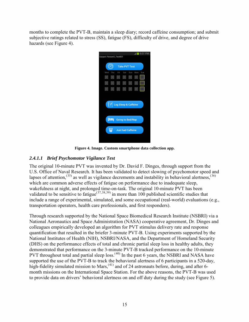
15

months to complete the PVT-B, maintain a sleep diary; record caffeine consumption; and submit subjective ratings related to stress (SS), fatigue (FS), difficulty of drive, and degree of drive hazards (see Figure 4).

Figure 4. Image. Custom smartphone data collection app.

2.4.1.1 Brief Psychomotor Vigilance Test The original 10-minute PVT was invented by Dr. David F. Dinges, through support from the U.S. Office of Naval Research. It has been validated to detect slowing of psychomotor speed and lapses of attention,(35) as well as vigilance decrements and instability in behavioral alertness,(36) which are common adverse effects of fatigue on performance due to inadequate sleep, wakefulness at night, and prolonged time-on-task. The original 10-minute PVT has been validated to be sensitive to fatigue(37,38,39) in more than 100 published scientific studies that include a range of experimental, simulated, and some occupational (real-world) evaluations (e.g., transportation operators, health care professionals, and first responders).

Through research supported by the National Space Biomedical Research Institute (NSBRI) via a National Aeronautics and Space Administration (NASA) cooperative agreement, Dr. Dinges and colleagues empirically developed an algorithm for PVT stimulus delivery rate and response quantification that resulted in the briefer 3-minute PVT-B. Using experiments supported by the National Institutes of Health (NIH), NSBRI/NASA, and the Department of Homeland Security (DHS) on the performance effects of total and chronic partial sleep loss in healthy adults, they demonstrated that performance on the 3-minute PVT-B tracked performance on the 10-minute PVT throughout total and partial sleep loss.(40) In the past 6 years, the NSBRI and NASA have supported the use of the PVT-B to track the behavioral alertness of 6 participants in a 520-day, high-fidelity simulated mission to Mars,(41) and of 24 astronauts before, during, and after 6-month missions on the International Space Station. For the above reasons, the PVT-B was used to provide data on drivers’ behavioral alertness on and off duty during the study (see Figure 5).

16

Figure 5. Screenshots. PVT-B performed on the smartphone data collection app.

2.4.1.2 Sleep and Caffeine Logs In addition to wearing an actigraph device, participants completed a daily sleep diary providing inputs related to sleep timing and self-reported sleep quality (including naps) and caffeine use. The sleep diary aided in interpreting the actigraph data, while providing an opportunity to collect data related to participants’ perceptions about their sleep quality and their caffeine consumption (see Figure 6).

Figure 6. Screenshots. Sleep diary and caffeine log performed on the smartphone data collection app.

17

2.4.1.3 Karolinska Sleepiness Scale and self-reports related to stress, fatigue, difficulty of drive, and degree of drive hazards

After completing each PVT-B, participants completed the KSS and provided subjective ratings (based on their perceptions) related to their stress level (rated on the SS), fatigue level (rated on the FS), the difficulty of their drive, and safety hazards experienced during their drive. The KSS and the above-listed self-reports of fatigue, stress, difficulty of drive, and safety hazards experienced were used in the 2014 field study on the HOS restart provision.(42) The KSS has been widely used in the literature as a subjective assessment of alertness (see Figure 7). The KSS is a 9-point Likert-type scale ranging from “extremely alert” to “extremely sleepy.” The FS is a 5-point scale ranging from “alert” to “tired.” The SS is a 5-point scale ranging from “not stressed” to “very stressed.” The difficulty of drive scale is a 5-point scale ranging from “easy” to “difficult.” The degree of drive hazards scale is a 5-point scale ranging from “few” to “many.”

Figure 7. Screenshots. KSS and self-reports related to stress, fatigue, difficulty of drive,

and degree of drive hazards, performed on the smartphone data collection app.

2.4.2 Issues Encountered with Smartphone-based Measures During the study, there were 21 instances of a smartphone being lost or damaged. When smartphone data (i.e., PVT-B, sleep diary, or driver ratings) were not uploaded to the study data server via a participant’s mobile data link, a member of the study team contacted the study participant to determine smartphone device status. Once the smartphone was verified to be lost or damaged, the study team couriered a replacement device to the study participant. In the time between damage to or loss of the smartphone and receipt of their replacement smartphone, participants were instructed to provide data on all other available study measures. The total amount of data lost to smartphones being lost or damaged constituted 440 data collection days (or 1.4 percent of the total smart phone measures).

18

2.4.3 Preexisting Health/Medical Conditions The background survey questionnaire (Appendix B) was administered to drivers during study enrollment. This questionnaire requested anthropometric measures (i.e., height, weight, and age) and data related to existing health conditions that were used as covariates in the analyses.

19

3. METHODS AND APPROACH Below is a description of the procedures and methods used to complete this study. The aim was to provide these methods in chronological order (as they were initiated during this study), but there may be some overlap of activities.

3.1 OVERVIEW

The study used a naturalistic approach—defined as an “unobtrusive observation or observation taking place in a natural setting”(43)—to evaluate the impacts of Sections 395.3(c) and 395.3(d) of Title 49, Code of Federal Regulations on CMV drivers. Specifically, the potential effects of 1) a 1-night restart relative to a 2-night restart and a more-than-2-night restart and 2) the potential effects of a restart taken in less than 168 hours versus a restart taken in at least 168 hours were evaluated relative to selected operational, safety, health, and fatigue outcomes. The study team enrolled a stratified convenience sample spanning the industry in terms of fleet size (small, medium, and large), type of operation (long-haul, regional, and short-haul), and industry sector (flatbed, refrigerated, tank, and dry-van) to enhance the generalizability of study findings. Participants were observed over the course of 5 months.

3.2 INSTITUTIONAL REVIEW BOARD

As required for all studies involving human subjects, the study team submitted an application to the Virginia Tech Transportation Institute (VTTI) Institutional Review Board (IRB) for their review and approval. The application included the research protocol, which provided a detailed description of all study tasks, data confidentiality, and data access. The application also contained an Informed Consent Form (ICF) to be signed by each participating driver. See Appendix C for one of the four different versions of the ICF (different versions of the ICF were created to account for presence of an ELD, presence of the BigRoad app, and significant travel to an installation site) and the VTTI IRB approval letter. The ICF outlines the study objectives and methods, data confidentiality, any possible risks, compensation, and the rights of the participant (including freedom to withdraw from the study at any time, for any reason). No human subject activities were conducted until IRB approval was received on February 18, 2015 (VTTI IRB# 15-063).

3.3 RECRUITMENT

3.3.1 Sampling Plan Taking advantage of the within- and between-driver design, a sample size of 199 has 80 percent power to detect a standardized effect size of 0.2 (mean difference divided by the standard deviation of within-driver differences) using a paired t-test with a 0.05 two-sided significance. A standardized effect size equal to 0.2 is typically considered small in the behavioral sciences.(44) However, effect sizes of this magnitude still have potentially important public health policy implications when applied to populations. Inclusion criteria were used to enrich the sample with regard to drivers expected to contribute both 1-night restarts and 2-or-more-night restarts.

20

However, drivers contributing only 2-or-more-night restarts still contribute statistical power to the comparisons in the mixed-model analyses. The target enrollment was specified in the approved study plan as 207 drivers, which is larger than 199. The number of drivers in excess of 199 helps to make up for any loss of power arising from some drivers contributing only more-than-2-night restarts. By the end of the study, 235 drivers had contributed at least 1 sampling unit for analysis. In summary, enough drivers were included in the study to detect with adequate statistical power relatively small differences in outcomes between sampling units varying in provision use.

For the results to be generalizable to the widest range of driving operations, drivers were to be recruited from small, medium, and large carriers involved in short-haul, regional, and long-haul operations on different truck types, including flat-bed, refrigerated, tank, and dry-van to the extent practicable. Each of the subgroups was represented to the extent feasible.

Below are the operational definitions for the industry segmentations:

• Carrier size: – Small: 1‒50 power units. – Medium: 51‒500 power units. – Large: more than 500 power units.

• Type of operation: – Short-haul: the driver normally operates within a 100 air-mile radius of the driver’s

home terminal. – Regional: the driver normally operates beyond a 100-air mile radius and up to 250

air-mile radius of the home terminal. The trip normally involves a single day—out and back to the home terminal.

– Long-haul: the driver normally operates beyond a 250 air-mile radius of the driver’s home terminal. The driver operates away from the home terminal for multiple days and the trip involves single or multiple loads.

• Industry sector (definitions used in the Fatality Analysis Reporting Systemiv and General Estimates Systemv): – Flat-bed: flat surface above rear tires; may have a front bulkhead and stake or strap

accommodations (including car hauler). – Refrigerated: a refrigerated and insulated box trailer. – Tank: cylindrical for liquid transport (including cement trucks). – Dry-van: fully enclosed with hard or soft sides and side and/or rear doors.

iv http://www.nhtsa.gov/FARS v http://www.nhtsa.gov/Data/National+Automotive+Sampling+System+(NASS)/NASS+General+Estimates+System

21

3.3.2 Industry Outreach The study required recruitment of carriers and individual driver participants from participating carriers. The study team used existing industry contacts to communicate with drivers and trucking companies in an effort to recruit drivers at their respective fleets. This involved sending 1,143 direct emails and making 244 direct phone calls to drivers and carriers. A wide variety of organizations were contacted to solicit their support in recruiting drivers for the study. These included the following organizations:

• Alliance for Driver Safety & Security.

• American Trucking Associations.

• American Transportation Research Institute.

• California Construction Trucking Association.

• California Trucking Association.

• Commercial Vehicle Safety Alliance.

• International Brotherhood of Teamsters.

• National Association of Small Trucking Companies.

• Owner Operator Independent Drivers Association.

• Tennessee Trucking Association.

• Transportation Trades Union.

• Washington State Trucking Association.

• Western Trucking Alliance.

• Women in Trucking.

The study was advertised on the Dave Nemo Open Road Channel Radio Show (every other Monday morning from 9–10 a.m. at Satellite Radio XM 171 or Sirius 147) throughout the recruitment period. The study team also visited the Mid-America Trucking Show in Louisville, KY from March 31 to April 2, 2015.

3.3.3 Carrier Participation After carriers provided a commitment to support the study, the study team worked closely with senior management and operational personnel to review company HOS data (if available) and/or driver self-report data to identify drivers who met the following criteria:

• Held a valid Class A commercial driver’s license (CDL) during the course of participation.

• Worked more than 60 hours per week (at least occasionally).

• Completed drives in the day and night.

22

• Used 1-night, 2-night, or more-than-2-night restarts and/or took restarts more frequently than 168 hours.

The study team also asked potential participants if they planned on continuing to work under the above conditions. Every effort was made to coordinate with the dispatchers and carrier operational staff to advertise the study to drivers who met the study criteria. In support of driver recruitment, two standardized posters were created (one directed at carriers and one directed at drivers) that provided details about the study (see Appendix D).

3.3.4 Web-based Screening and Enrollment of Drivers The recruitment efforts described above directed carriers and drivers to the official recruitment Web site (www.RestartStudy.com). The recruitment Web site (see Appendix E for screenshots) provided an overview of the study and an opportunity for drivers to register to be considered as participants. Interested drivers answered several screening questions designed to assess whether carriers/drivers met the study inclusion criteria (as shown above). Drivers were also asked to provide contact information so that the study team could later contact them. A total of 5,176 unique visitors accessed the recruitment Web site—757 of these visitors completed or partially completed the screening questionnaire, and 379 met the study criteria. Ultimately, 242 drivers were empaneled in the study. Table 8 shows the distribution of empaneled drivers across the various industry segmentations.

Table 8. Driver empanelment by industry segmentation.

Industry Segmentation Target N for Analysis Drivers Empaneled

Drivers Contributing ≥ One Sample Carriers

Small 110 47 43 45 Medium 20 76 73 34 Large 77 119 119 16

Total 207 242 235 95 Long-haul 95 192 187 90 Regional 56 32 31 8 Short-haul 56 18 17 3

Total 207 242 235 101* Dry-van 119 133 130 55 Flat-bed 33 35 35 14 Refrigerated 33 63 59 26 Tank 22 11 11 11

Total 207 242 235 106*

*A total of 95 different carriers participated in the study. Some carriers provided drivers from more than one industry segment.

3.3.5 Empanelment Logistics Due to the geographic distribution of participants and varying driver schedules, the process of empaneling drivers and equipping vehicles required a great deal of coordination. To support timely hardware installation and in-person informed consent briefings, the study team offered a variety of empanelment options. Drivers had the option of attending a scheduled vehicle

23

installation and briefing session at 1 of 11 selected technology deployment locations/convenient operational centers. Alternatively, the empanelment team scheduled empanelment trips—on a case-by-case basis—to carriers employing eight or more participants. Finally, seven participants were empaneled on site at the Mid-America Trucking Show.

The technology deployment locations/convenient operational centers used for empanelment purposes during this study included: Allentown, PA; Atlanta, GA; Blacksburg, VA; Freemont, CA; Memphis TN; Ontario, CA; Philadelphia, PA; Riverside, MO; Seattle, WA; and Warrenville, IL.

3.4 DRIVER RETENTION

To maximize participant retention and compliance with study protocols, the study measures were collected in near-real-time and reviewed daily to detect missing, spurious, or corrupt data, or device hardware or software failures. When a protocol deviation was detected (e.g., the OBMS camera lens was obstructed), a member of the study team contacted the participant to understand the source of the problem and to provide corrective feedback. Immediate feedback was essential for ensuring driver compliance with the study protocol throughout the entire data collection phase of the study.

Drivers were reimbursed for their efforts in support of the study. Driver compensation was based on completion rates of study activities on a pro rata basis according to the following schedule. Drivers could receive up to $2,166 if they participated for the entire 5 months of this study, and if they completed all assessments as requested. Participants received three payments over the course of their participation as follows:

• $75 at the initial meeting for signing the ICF and completing the health assessment. This was paid in cash or check at the time of the meeting (if possible), or a check was mailed to the participant’s home within 1 week. – $50 for attending the initial briefing and signing up for the study. – $25 for completing a health assessment questionnaire during the initial briefing.

• A second payment of up to $1,891 for participating in the study if they contributed data for 5 full months. They received this payment by check mailed to their home within 30 days of completing participation. – Up to $1,606 for 22 weeks of participation. Participants were asked to complete three

smartphone assessments, three times per day, to receive the following payment: › $3 per assessment × three assessments/day = up to $9/day. › $9/day × 7 days in a week + $10 bonus for completing all assessments in a week

= up to $73/week. › 22 weeks × $73/week = $1,606 for completing all assessments.

– $25 for participating in a debriefing phone call at the end of the study. – $260 bonus for completing 5 full months of participation.

24

• Drivers received a third (and final) payment of up to $200 if they returned all three pieces of equipment. Pre-paid packaging materials were sent to participants at the end of the study. Participants received this payment by check, which was mailed to their home within 30 days of receiving the equipment: – $50 for returning the actigraph device. – $50 for returning the smartphone. – $100 for returning the OBMS.

If a participant elected to withdraw from the study or if their employment ended (and the new employer would not authorize their involvement in the study), that participant was compensated for their participation up to that point.

3.5 PARTICIPANT BRIEFING

3.5.1 Pre-study Briefing During the pre-study briefing, participants were given a detailed explanation of all of the study procedures and the informed consent process. These pre-study briefings were held at one of the participating carrier’s terminal locations, the Mid-America Trucking Show, or at one of the other installation locations across the United States. The following activities took place during the pre-study briefing:

• Participants were asked to confirm that they had a valid CDL.

• Participants were assigned a smartphone and an actigraph device.

• Researchers took a digital photograph of each participant’s face to assist with identification when reviewing video data.

• Participants completed the background survey, either on paper or using a researcher’s computer.

• Participants completed a W9 tax form for subject reimbursement.

• Participants were trained to use the various smartphone apps (i.e., PVT-B, FS, SS, KSS, caffeine log, difficulty of drive, degree of drive hazards, and sleep diary), the BigRoad app (if their truck did not have an existing enterprise-grade ELD), and how to download the data from their wrist actigraph devices.

• Participants also had the opportunity to ask any questions.

3.5.2 Weekly Debriefs Throughout the study, members of the study team communicated (by phone and/or email) with drivers on an as-needed basis and during weekly scheduled debriefs. The purpose of this contact was to receive clarifications from drivers regarding misaligned data, to ask questions, and to provide feedback about missing data, study equipment problems, or study procedures that were not followed correctly.

25

During these weekly debriefs, study participants were also asked to predict their next restart (e.g., 1-night, 2-night, or more-than-2-night restart). The reason for this selection (operational imperative versus driver preference) was also elicited, using the following wording:

1. Largely my decision, but based on work requirements.

2. Largely my decision, but based on personal preference.

3. Largely my company’s decision.

4. Largely due to Federal regulations.

This allowed comparisons between driver predictions and actual restart conditions. This was done as a measure of selection bias.

3.5.3 Final Debriefing The final participant debriefing was scheduled following the 5-month data collection period or when participants exited the study. Participants returned the equipment (smartphone, actigraph device, and OBMS) to the study team via mail using pre-paid packaging. Those drivers who had an existing Lytx OBMS installed in their truck prior to the study did not return the OBMS and automatically received the $100. The study team received final clarifications from drivers regarding data that did not align, asked questions, and provided feedback about missing data, study equipment problems, or study procedures that were not followed correctly. In addition, study participants had an opportunity to ask questions about the study or express any concerns.

3.6 VEHICLE INSTALLATION

The study team equipped participants’ vehicles with an OBMS. This installation took place after the participant pre-study briefing. The installation process was fairly easy and took approximately 30‒60 minutes. As shown in Figure 1, the OBMS was installed in a location that did not impede the driver’s view of the forward roadway. As shown in Figure 2, the OBMS was mounted so that it would provide a good view of the forward roadway and the driver (from the driver’s lap to the top of the driver’s head), thereby allowing data analysts to code fatigue and/or engagement in any non-driving tasks (e.g., texting, eating, etc.).

3.7 DATA COLLECTION

Once participants signed the ICF, received their assigned study equipment/training on how to use the apps and actigraph devices, and their vehicles were fully installed with the required equipment (OBMS and possibly an ELD), data collection began. Participating drivers drove an instrumented vehicle for up to 5 consecutive months. Below is a description of how the data were collected, reduced, and transmitted.

3.7.1 Onboard Monitoring System Data The technology vendor was responsible for all OBMS data collection and reduction. The encrypted video and quantitative data from all instrumented trucks were automatically sent to the technology vendor via cellular transmission. The received data were reviewed, reduced (i.e., data

26

analysts marked the presence of specific variables pertaining to each event), and uploaded to a secure server.

3.7.1.1 Data Reduction Data analysts underwent an extensive 5-week training regimen prior to reducing “real” data. The technology vendor currently sees 97-percent reliability with a 95-percent confidence interval using their standard data reduction protocols. The study team added additional reduction variables, including enhanced fatigue, traffic density, and reaction time to precipitating event. To ensure the additional reduction variables were being reduced correctly, the study team requested that the first 500 events (SCEs and false safety triggers) be reduced by two data analysts and one senior trainer (if necessary, to break any discrepancies between the two data analysts) and that the results be sent to the research team to calculate reliability. At the quarter point of data reduction (25 percent of all events reduced), the study team evaluated reliability on events reviewed by two reductionists. Reliability at both checkpoints was satisfactory; thus, no retraining was required and data reduction commenced as planned. Random reliability checks were also completed on validated events (events that overlapped with the driver’s duty status via the ELD and truck number) by comparing the participating driver’s picture to the video image. These random checks were 100 percent accurate. The technology vendor’s data analysts performed blind data coding, in that they did not know what type of restart each of the participants had taken.

Once the data were received, a trained data analyst reviewed the data to determine if it represented a valid SCE or a false safety trigger (e.g., hitting a pothole in the street, driving on a bumpy road, etc.). False safety triggers, though normally not reduced, received the same reduction as SCEs except for the reaction time to predicating event variable (noted below). Standard data reduction involved reviewing the video and recording the trigger type, outcome, root cause, demeanor, risky behaviors, and adverse weather conditions (if necessary). Additional reduction questions were added in the study, including enhanced fatigue coding, traffic density, and reaction time to precipitating event. The date, time, fleet number, and driver identification (ID) number were automatically tagged to the SCE and false safety trigger. Data analysts completed their reduction of the SCEs and false safety triggers approximately 1–14 days from the time the data were recorded by the OBMS in the instrumented truck and uploaded to the technology vendor’s secure server.

3.7.1.2 Fatigue-coded Safety-critical Events and False Safety Triggers from the Onboard Monitoring System

“Observer rating of drowsiness” (ORD)vi is a well-established method for measuring fatigue using video data to assess facial features and body language.(45) However, ORD requires at least 1 minute of video and the “average” score over that minute is used to assess fatigue. For example, a driver could show significant signs of fatigue earlier in the video, but appear to be less fatigued later in the video, as it is common for people to drift in and out of fatigue, but

vi ORD demonstrated good intra- and inter-rater reliability in that the measure correlated highly (r = +0.7 to 0.9) with eye closure measures such as PERCLOS (percentage of time that the eyes were closed 80 percent or more) and mean percent eye closure (AVECLOS).

27

remain fatigued overall. In this example, the driver would be coded as showing significant signs of fatigue even though he/she showed periods of lower fatigue in the video.

The video length in this study was 12 seconds, and only the first 8 seconds of video could be used, as the precipitating event (e.g., swerve in response to a lead vehicle stopping or driving over rough road if it was a false safety trigger) could increase the driver’s arousal. Thus, ORD was not possible and data analysts at the technology vendor were trained to perform an enhanced analysis of fatigue (conducted on all SCEs and false safety triggers). The length of the video only allowed for a determination of acute fatigue, as less subtle (but common) signs of fatigue could not be determined reliably with 8 seconds of video.

Data analysts were instructed to watch the driver’s face and body language in the 8 seconds prior to the trigger threshold during SCEs and false safety triggers. A bivariate measure of fatigue was used given the limited amount of video data. After watching the video data, data analysts employed a rating to record the presence of acute fatigue using the following ratings:

• Fatigue (but not asleep): As a driver becomes very fatigued, slow eyelid closures usually occur. This is often accompanied by a rolling upward or sideways movement of the eyes themselves. The individual may also appear not to be focusing the eyes properly, or may exhibit a cross-eyed (lack of proper vergence) look. Facial tone will probably have decreased. Very fatigued drivers may also exhibit a lack of apparent activity, and there may be large isolated (or punctuating) movements, such as providing a large correction to steering or re-orienting the head from a leaning or tilted position. Drivers are close to falling asleep and usually exhibit prolonged eyelid closures and similar prolonged periods of lack of activity. There may be large punctuated movements as they open their eyes.

• No fatigue: May exhibit some or none of the signs above; however, the driver did not meet the criteria noted above for fatigue.

• Asleep: Drivers are falling asleep if they exhibit prolonged eyelid closures (3 seconds or more). There may be large punctuated movements as they transition in and out of intervals of dozing. A driver cannot be coded as fatigued and asleep.

• Unknown: It was too dark to make out the driver’s eyes, the view was obscured, or the camera malfunctioned.

• Not available (or N/A): A parked vehicle was struck or was being loaded; a driver bumped the camera when parked.

The overall inter-rater reliability (i.e., agreement between the two data analysts) for the enhanced fatigue reduction was 88.3 percent.

3.7.1.3 Traffic Density All SCEs and false safety trigger events were reviewed by the data analysts to determine traffic density. Traffic density was a qualitative measure used to relate the quality of traffic service (in terms of traffic flow and speed). There were three levels of traffic density: low, medium, and high. Low density was when traffic flowed at or above the posted speed limit and motorists had

28

complete mobility between lanes or maneuverability within the traffic stream was only slightly restricted. Medium density was where the ability to maneuver through lanes was noticeably restricted and lane changes required more driver awareness. Speeds were slightly decreased as traffic volume slightly increased. Freedom to maneuver within the traffic stream was much more limited. High density was when traffic flow became irregular and speed varied rapidly because there were virtually no usable gaps to maneuver in the traffic stream and the speeds rarely reached the posted limit. This also included instances where every vehicle moved in lockstep with the vehicle in front of it, with frequent slowing required (i.e., traffic jam). The overall inter-rater reliability for the traffic density reduction was 85.9 percent.

3.7.1.4 Reaction Time to Precipitating Event All SCEs were reviewed by the data analysts to determine the driver’s reaction time to the precipitating event. A precipitating event was the state of environment or action that began the SCE sequence under analysis. In other words, what environmental state or what action by the subject vehicle, another vehicle, person, animal, or non-fixed object was critical to this vehicle becoming involved in the SCE. The driver’s reaction to the precipitating event was when the driver was first seen to recognize and begin to react to the SCE occurring. The number of frames (each frame is 0.25 seconds) between the precipitating event and the driver’s reaction to the precipitating event was used to determine the driver’s reaction time. No reduction was performed on SCEs with a speeding trigger, as there was no precipitating event. No reliability checks were performed on this variable; the average value of the two data analysts’ results was used as the final value.

3.7.1.5 Data Transmission Once data reduction and reliability checks were completed, the reduced data set was sent to the study team for analysis. The data set was stored on a secure, password-protected server. Contained in the data set was the categorical reduction for each false safety trigger and SCE, including:

• A unique time/date.

• GPS location of the event.

• Carrier ID number.

• Unique driver ID number.

• Unique event ID number.

• Trigger type.

• Severity of SCE (including a crash, near-crash, or other event).

• The categorical reduction (including the standard Lytx protocol and the additional reduction variables).

• The maximum kinematic values.

29

3.7.2 Smartphone App Data Participants used the custom smartphone data collection app every day throughout the 5 months of data collection at the following points in time:

• At the beginning of a duty period before driving, on a smartphone (approximately 10 minutes): – Driver completed sleep/wake/duty diary. – Driver performed a 3-minute behavioral alertness test (PVT-B). – Driver rated fatigue on a fatigue scale (FS). – Driver rated sleepiness on the Karolinska Sleepiness Scale (KSS).

• During a break from driving, about halfway through a duty period, on a smartphone (approximately 5 minutes): – Driver performed a PVT-B. – Driver rated stress (SS). – Driver rated fatigue (FS). – Driver rated difficulty of drive. – Driver rated degree of drive hazards. – Driver rated sleepiness (KSS).

• At end of a duty period after driving, on a smartphone (approximately 10 minutes): – Driver performed a PVT-B. – Driver rated fatigue (FS). – Driver rated sleepiness (KSS). – Driver completed sleep/wake/duty diary.

Participants also used the app during restart days to provide the same measures at a time within 2 hours of waking, about midway through the waking period, and within 2 hours of sleeping. The app detected motion and did not allow participants to complete the smartphone-based PVT-B while the vehicle was in motion. For team drivers, the study team provided instructions to the off-duty driver in the sleeper berth to complete assessments at the same time as his or her driving partner before the drive, after the drive, and when taking a break.

3.7.2.1 Data Transmission and Reduction Smartphone app data (PVT-B, sleep diary, caffeine log, etc.) were collected and transmitted in real-time via secure mobile data link to a server. Raw PVT-B data, sleep diary and caffeine log entries, and other questionnaire data were parsed and secondary metrics calculated. Data quality control analyses included programmatic scripts and manual review to detect missing, spurious, or corrupt data, and device hardware or software failures. Weekly data quality reports were generated to support weekly participant telephone debriefings.

30

After the data quality control process was completed, de-identified data were formatted and transmitted for statistical analysis. Data were automatically uploaded and securely transferred to the research team to support near-real-time data collection, quality control, and variables extraction.

3.7.3 Electronic Logging Device Data ELD data were collected using a variety of approaches based on the carrier’s deployed ELD solution. In cases where a carrier did not have an ELD solution, one was provided during the study (the BigRoad app with DashLink was delivered on the study-issued smartphone).

3.7.3.1 Data Transmission and Reduction The study team developed an ELD data flow plan for each carrier based on the technology used and a carrier-specific work flow. The goal was to collect ELD data as frequently as possible in a manner that had the smallest impact on carriers. ELD data were collected and variables related to driver status were extracted (i.e., timing and duration of driving, working, sleeper berth, and off-duty) to provide the primary independent study measure in the aggregate analysis.

3.7.4 Actigraph Data Participants wore ActiGraph’s wGT3X-BT actigraph devices on their wrists during the study to measure sleep timing and quantity. The rechargeable battery lasted 7‒14 days with wireless transmit mode enabled. Each participant received a universal serial bus charger with an alternating current wall adapter and 12-volt cigarette lighter adapter to enable charging in the vehicle. Devices took approximately 2 hours to charge. Participants were instructed to remove and charge the actigraph device once per week (e.g., every Wednesday). As the data were uplinked in near-real-time (i.e., daily), the study team was aware of any problems with the device, such as a dead battery, and contacted the participant promptly to troubleshoot the problem.

3.7.4.1 Data Transmission and Reduction Actigraph data were transmitted in real-time via secure mobile data link to the study team’s server. Raw actigraph data were parsed and secondary metrics calculated. Data quality control analyses included programmatic scripts and manual review to detect missing, spurious, or corrupt data, and device hardware or software failures. Weekly data quality reports were generated to support weekly participant telephone debriefings. Data were automatically uploaded and securely transferred to the study team to support real-time data collection, quality control, and variable extraction.

Sleep was manually scored by a research assistant who received training in scoring actigraph-based sleep records. Sleep was scored in 1-minute epochs for every minute during participants’ data collection period. Sleep was scored as either “awake,” “asleep,” or “unknown” based on data from the actigraph device and the sleep diary. These data were cross-referenced with ELD data to ensure data consistency. Each epoch was additionally assigned a code indicating which data sources contributed to the determination for that epoch according to the rules in Figure 8. For example, if a driver recorded a sleep period in the smartphone-based sleep log and the data from that driver’s actigraph device also indicated sleep, then all of those 1-minute epochs would

31

be scored as sleep. If a driver did not provide a sleep entry in the smartphone-based sleep log for a given 24-hour period, but the data from that driver’s actigraph device indicated sleep, then the period of time would be scored as sleep. If the actigraph indicated continuous movement it would be scored as wakefulness. If a driver did not provide a sleep entry in the smartphone-based sleep log for a given 24-hour period, and the actigraph record for the same 24-hour period was missing data (e.g., due to battery failure), the adjudicated scoring would indicate missing data.

Figure 8. Chart. Rules for adjudicated sleep scoring using participants’ actigraph records and sleep diary

logs.

3.8 METHODOLOGY LIMITATIONS

The smartphone required daily battery recharging, and a driver could also use it for data input and submission by plugging it into a charger. The actigraph device required a battery recharge every 7–14 days. When the battery failed to be recharged, data were not received and the driver was sent a replacement actigraph device with a new battery. Study staff contacted drivers weekly regarding the charging status of the devices and any replacement equipment being sent to them. Sections 2.4.2 and 2.3.1 detail the data acquired with the devices and the extent to which data were lost due to battery discharge or damage to the devices.

32


33

4. ANALYSIS PLAN AND DATA PROCESSING The study used a naturalistic approach defined as an “unobtrusive observation or observation taking place in a natural setting”(46) to evaluate the impacts of Sections 395.3(c) and 395.3(d) of Title 49, Code of Federal Regulations. Specifically, the study addressed two HOS provisions:

• First, potential effects of a 1-night restart duty cycle, relative to a 2-night or more-than-2-night restart duty cycle.

• Second, the potential effects of taking a restart in 168 hours or more following the beginning of the prior restart compared to taking a restart in less than 168 hours. These were evaluated relative to selected operational, safety, health, and fatigue outcomes.

The ELD data generated from each driver were partitioned into sampling units (SUs). SU partitioning, as executed, was required to meet the study objectives, and is consistent with the study work plan.(47) This section describes the conceptual model used and defines the primary concepts implemented using a computer-based algorithm.

4.1 CONCEPTUAL MODEL USED TO PARTITION ELECTRONIC LOGGING DEVICE RECORDS INTO SAMPLING UNITS

Figure 9 summarizes the conceptual model that guided the data reduction procedures used to partition each driver’s ELD data into discrete SUs. By definition, each SU was comprised of a restart period (R), followed by a duty or non-restart period (NR). The letter ‘t’ signifies a specific sampling unit [SU(t)], and by extension, its corresponding R(t) and NR(t). A central component to this model was that every R(t) was classified according to the restart provisions described above.

Figure 9. Schematic. Organization of ELD data into SUs, restart periods, and work periods.

The distributions of the operational, safety, health, and fatigue outcomes determined during NR(t) were compared among SU(t)s that had been categorized according to provision use associated with the corresponding R(t). In some cases, outcomes defined within R(t) itself were relevant (e.g., mean daily sleep during R(t)).

The notation defined above was formally extended to identify specific drivers, i = 1 to ND, as in SU(i,t), where ND was the number of enrolled drivers contributing at least one valid SU(t).

34

Among the 242 enrolled drivers, ND = 235 contributed at least one SU(t). The reasons for lack of contributing at least one sampling unit are summarized below.

In this way, the follow-up periods as reflected in the ELD data for each driver were partitioned into sampling units SU(i,t) (i=1 to ND, t=1 to T) and each SU(i,t) was constructed to include exactly one R(i,t) period followed by exactly one NR(i,t) period. For example, R(3,5) denotes the 5th restart period for driver 3 and NR(100, 10) is the 10th non-restart period, that is, the 10th work duty cycle for driver 100.

4.1.1 Electronic Logging Device Data Handling The ELD data were collected from participating carriers and independent drivers as necessary. The ELD records were delivered in varying formats, which were converted into a standardized format. Consistency checks and other methods of validation (described above) were conducted. Each file contained date-times of ELD status changes recorded by the driver in UTC and home terminal time, as well as a truck ID number necessary for cross-linking with a specific OBMS installed in an instrumented truck. This cross-linking was necessary for defining “instrumented hours driving” for each SU(t) included in the data analysis to obtain more accurate measures of “exposure” for the SCEs.

4.1.2 Electronic Logging Device Sampling Unit Identification Algorithm The driver-specific ELD history files served as the input for the ELD SU identification algorithm. This algorithm was based on the use of Statistical Analysis Software (SAS) Proc Expand. It begins by expanding the set of status change onsets into a minute-by-minute chronology in which each minute is classified according to the ELD status types of:

1. Driving.

2. On-duty.

3. Off-duty.

4. Sleeper Berth.

These ELD status types were further simplified to “working” (driving or on-duty) and “not working” (off-duty or sleeper) for the purpose of implementing the algorithm. It is important to highlight the definition of the ELD status “sleeper.” This was time spent in the truck’s sleeper berth, but does not necessarily imply the driver was actually sleeping. It only indicates the driver reported he or she was in the truck’s sleeper berth, which was classified—along with “off-duty”—as “not working” time.

The ELD data that serves as input in the algorithm includes confidential information protected by the VTTI IRB. These data are analogous to video files that contain personally identifying information. Thus, the protected components of the ELD data are not included in the public data set.

To summarize, the ELD SU identification algorithm was used to determine the onset and completion of each R(i,t) and NR(i,t) for each driver. The R(i,t)s were identified sequentially as any period in which there were at least 34 consecutive hours in which the ELD status indicated

35

“not working.” The interval of time until the onset of the next 34 consecutive hours (minimum) of “not working” was then defined as NR(i,t). By construction and consistent with regulations, the R(i,t)s could include only “off-duty” or in “sleeper.” An ELD status of “on-duty” or “driving” would necessarily end R(i,t). NR(i,t)s could consist of all four possible ELD status types (i.e., on-duty, driving, off-duty, and sleeper).

4.1.3 Quality Assurance Procedures The raw ELD data files contained information reflecting driver behavior that could be used to identify specific drivers. Therefore, the raw ELD records collected during this study are protected and cannot be made available to the general public. Consequently, the study team determined it was essential to validate the output of the ELD sampling unit identification algorithm. In general, there are two key methods to validate such programming: “double programming” and “code review.” Both methods were used to ensure the outputs from the algorithm were valid, including the partitioning of the ELD records into sampling units and determining the beginning and end of every restart period and duty period. Double programming was accomplished by having the algorithm independently programmed by two different organizations within the research team using different programming platforms. Initially, one member of the research team programmed the algorithm using MATLAB (a proprietary programming language). Results from these preliminary findings were provided to the study team in an ongoing fashion. Simultaneously, another member of the research team programmed the algorithm in SAS with special attention as to how outcome variables could be assigned to each restart and duty period as appropriate. As the SAS algorithm matured, results were compared to those produced by the MATLAB algorithm. Differences in results between the algorithms were investigated and resolved in an ongoing fashion, including substantial discussion between responsible parties. The same process was used for counting the SCEs. At the end of this process, quality metrics revealed greater than 99 percent agreement on all relevant variables. In addition to double programming, code review was performed on multiple occasions. Code review involved the primary programmer explaining to another programmer the logic of key program elements. This method is effective in identifying code segments with potential logical problems and included line by line inspection of key elements in the algorithm. Similar quality assurance checks were performed on the other outcome variables (e.g., actigraphy, sleep diary, KSS, etc.). This included comparing counts of testing bouts (e.g., PVT-B and driver-reported outcomes) from the source data to the numbers of testing bouts included in the final analysis data sets produced by the analysis team. Finally, in addition to the above, the study team reviewed marginal distributions of outcomes prior to unblinding (see Section 4.2) to assess scientific and logical plausibility. This process was repeated after unblinding. In total, these quality assurance procedures ensured the analyses were performed on the highest quality data possible.

4.2 BLINDING OF OUTCOME VARIABLES TO AVOID ANALYSIS BIAS

A number of decisions and assumptions were made to implement the data reduction plan and the analysis plan. To avoid conscious (or subconscious) bias, the study team decided to keep the outcome data, including PVT-B outcomes; driver-reported responses pertaining to sleepiness, fatigue, stress, hazards and difficulty of drive; adjudicated estimates of sleep duration; and

36

OBMS event data blinded from the primary study statistician, the project technical lead, and other members of the study team, and from FMCSA. This was implemented by having the primary study analyst randomly sort outcome data before attaching outcomes to the SU(t)s when constructing the preliminary analysis datasets. In this way, the distributions of outcome variables could be reviewed and beta testing of descriptive and statistical analyses was performed without concern that decisions would bias the results in one direction or another. Only when all quality-related data decisions, such as exclusions of SUs from the analysis set and statistical models for testing primary hypotheses were specified, were the outcome variables unblinded with regard to the real SU(t) and associated provisions to which they belonged.

4.3 TRUNCATION AND EXCLUSION OF SU(T)S

In preliminary analyses, it was observed that some lengths of SU(t)s were several months long. There were several reasons for this. In some cases, this reflected the driver’s behavior (e.g., the driver simply did not have periods of at least 34 consecutive hours “not working,” preventing the algorithm from terminating the NR(t) period). In other cases, it was determined the driver did not log off his or her ELD prior to leaving work for an extended period, such as a vacation. Finally, regardless of the particular reason, the study team decided the maximum length of NR(t) should be 14 days. This length of time was long enough to capture outcomes during periods of time in which it was reasonably expected the provisions may have impacted the driver’s safety, fatigue, operations, and health. Moreover, there was little or no evidence that changes in behavior implied by provision use extend beyond 14 days for the outcomes of interest in this study. The 14-day truncation rule was observed to produce distributions that contained fewer outliers, likely due to artifacts in the ELD records.

4.3.1 Exclusions As described below, the ELD SU identification algorithm generally produced partitions of the ELD follow-up into SU(t)s with mean driving time and on-and off-duty times per day that had substantial face validity during R(t) and NR(t). However, in some cases, the NR(t)s appeared too short to provide a meaningful assessment of outcomes in general. Furthermore, when evaluating SCE rates, there was a further reduction in the estimated hours driving since only hours driving in an OBMS-instrumented truck provided “exposure time” for SCEs. Therefore, the following exclusion criteria were employed. All data from SU(t)s meeting any of the following criteria were excluded from the analysis to test the effects of the provisions on the outcome variables. Appendix I and Appendix J provide listings of excluded SU(t)s. In total, 315 of 3,602 SU(t)s were excluded (resulting in 3,287 sampling units) based on the following criteria (note that a driver could have had more than one of these exclusion criteria):

1. Exclude SU(t)s with total driving time less than 4 hours (154 exclusions).

2. Exclude SU(t)s with NR(t)s that were less than 1 day (270 exclusions).

3. Exclude SU(t)s with mean driving time per day more than 20 hours and total driving time more than 300 hours (2 exclusions).

4. Exclude SU(t)s with NR(t)s that were more than 87 days (2 exclusions).

37

4.4 PROVISION USE

The HOS data in the ELD files were similarly processed to determine the primary independent variables related to Section 395.3(c). To this end, each R(t) was classified according to whether the consecutive period of at least 34 hours included one period of 1–5 a.m. versus two or more such periods. To add clarity to the interpretations, the study team decided to also evaluate comparisons among SUs with one period of 1–5 a.m. versus those with exactly two such periods, versus those with three or more such periods. Similarly, to evaluate the impact of Section 395.3(d), each R(t) was classified according to whether the elapsed time from the initiation of the prior restart to the initiation of next restart was at least 168 hours or less than 168 hours.

4.4.1 Numbers of Nights Per Restart The number of nights in R(i,t) was determined by counting the number of 1–5 a.m. pairs that occurred during this time period. This allowed each SU(i,t) to be categorized as 1 night, 2 nights, or more than 2 nights. The impacts of Section 395.3(c) on selected operational, safety, health, and fatigue outcomes were assessed by comparing SUs with 1 night versus 2 or more nights, and by comparing SUs with 1 night to those with 2 nights (versus more than 2 nights).

4.4.2 Restart in at Least 168 Hours Versus Less Than 168 Hours For Section 395.3(d), provision use was determined according to the number of hours from the beginning of the prior restart, R(i,t-1), to the initiation of R(i,t). This time period was exactly equal to the length of SU(i,t-1), implying the first SU could not be categorized according to this provision. Therefore, the SU(i,t=1)s could not be used for the comparisons of SUs with less than 168 hours versus at least 168 hours, and when both provisions were evaluated simultaneously, such as in multivariable statistical models.

4.4.3 Determining Time of Day Time of day in the study was set to the driver’s home terminal time zone. If a driver changed jobs and home terminal time zones, then time of day was set to new home terminal time zone.

4.5 ONBOARD MONITORING SYSTEM EVENT LINKING AND “INSTRUMENTED HOURS DRIVEN”

Linking the thousands of captured SCEs and false safety triggers to participating drivers presented special challenges. The first challenge was dealing with SCEs and false safety triggers from drivers not participating in the study. If a SCE or false safety trigger occurred while a particular driver had an ELD status of anything but “driving,” it was concluded the OBMS was not capturing the study driver. These instances could include various situations, such as a mechanic driving the truck, team drivers (where only one of the team drivers participated in the study), or slip-seat drivers (where several drivers were driving several trucks). These SCEs and false safety triggers were not matched and were excluded from all analyses.

The second challenge involved a study driver driving a truck other than the OBMS-instrumented truck. Here “instrumented” means the participating driver was driving in a truck with an operational OBMS that was associated with that driver (at least during this time interval).

38

“Operational” means the OBMS was working as intended, with no reported technical issues. Each driver’s ELD file included a specific truck ID. Each SCE and false safety trigger was checked against the driver’s ELD status and specific truck ID.

The third challenge involved non-operational OBMSs. If the OBMS experienced technical issues or there was abuse/obstruction of the OBMS (e.g., camera was obscured), this was indicated for the event. These types of OBMS issues could render the OBMS unreliable for accurately capturing SCEs and false safety triggers. Some of these SCEs and false safety triggers required troubleshooting with the driver prior to being deemed reliable. These times were defined as non-instrumented driving time and not included in the denominators when determining SCE and fatigue-related false safety trigger rates. A separate file containing the dates a specific OBMS was non-operational/operational was provided. Upon resolution of the OBMS issue, driving time may have been considered “instrumented.”

The following strategy was used to link SCEs and false safety triggers to specific drivers. A key concept was that these events were linked to a specific OBMS (which was also linked to a specific truck ID). An SCE or false safety trigger was considered correctly linked to a specific driver if the following three conditions were met:

• Complete driver accounting in the “linking” document.

• ELD data included truck ID for that time period.

• SCEs and false safety triggers included a date-time stamp that matched the date-time stamp to a time in which it was known the driver was driving a truck with an operational OBMS. Indication of a non-operational/unreliable OBMS was considered not-instrumented time. This not-instrumented time ends with successful troubleshooting.

The linking document recorded the date of installation (and subsequent installation, if necessary) with the OBMS ID (and secondary or tertiary OBMS ID, if applicable). The criteria above were necessary and sufficient for determining the driving times per SU (during periods when participants were driving in instrumented trucks with fully operational OBMSs that accurately captured SCEs and false safety triggers). During driving times classified as “not instrumented,” SCEs and false safety triggers were not matched, but were not given counts of 0 for this time. Rather, the hours of driving exposure were reduced to accurately reflect the true “driving-while-instrumented” time. Similarly, for each SU, hours in which the OBMS was “not operational” were subtracted from total hours driving and a new variable was constructed—“total instrumented driving time per sampling unit.” This approach was also applied to single-truck, multiple-driver situations (e.g., team drivers and slip-seat drivers).

4.5.1 Summary of Approach for Defining Exposure to SCEs In summary, for each SU, the following numerators and denominators were determined. The numerator equals the number of “confirmed” SCEs or false safety triggers per SU. The denominator equals the number of “instrumented” hours driving per SU. “Confirmed” means it was known, based on the three criteria listed above, that the SCE or false safety trigger occurred while the specific driver was driving. “Instrumented” means the driver was driving in a truck with an operational OBMS that was associated with that driver (at least during this time interval).

39

4.6 MIXED-EFFECTS STATISTICAL MODELS

Formal statistical comparisons, including testing of the primary and secondary hypotheses concerning differences in expected outcome on the basis of provision use, were performed using linear(48,49) and non-linear(50) mixed-effects modeling. These analyses were performed using the SAS/STAT® procedures MIXED and GLIMMIX (version 9.4), respectively. The objectives of using the mixed modeling approach were to reduce potential bias and confounding arising from the observational naturalistic study design and to account for correlations among multiple outcomes from the same driver and among multiple outcomes observed within the same sampling unit.

Every model included a factor for the number of nights included in the restart period (1 night versus 2 nights versus 2 or more nights), use of the 168-hour provision, and a factor for restart nights by 168-hour provision interaction. Models also included a set of a priori selected covariates specified in the work plan. These covariates included age and body mass index (BMI) as continuous variables, and the following baseline categorical variables: prior participation in a fatigue management program, gender, marital status, diabetes, high blood pressure, insomnia, sleep apnea, pain experience, use of caffeine, and use of tobacco. Models also included two factors obtained prior to each restart period. These factors related to drivers’ planned number of restart nights on their next restart and the reason for this decision. Finally, models for outcomes collected multiple times per day included a time-of-day factor defined according to home terminal time:

• 12 a.m. (midnight) to 3:59 a.m.

• 4 a.m. to 7:59 a.m.

• 8 a.m. to 11:59 a.m.

• 12 p.m. (noon) to 3:59 p.m.

• 4 p.m. to 7:59 p.m.

• 8 p.m. to 11:59 p.m.

Using these covariates, estimated predicted mean values for type of provision use were weighted to reflect the characteristics in the obtained sample. Random effects were included in the mixed linear models to account for correlations among outcomes from the same driver and to account for any “extra” correlation among multiple observations within the same sampling unit for outcomes assessed multiple times. Linear mixed models were used for all continuous and ordinal outcomes. Generalized mixed-effects models were used for outcomes expressed as counts or rates. Details regarding the construction of the mixed-effects models are provided in Appendix K.

4.7 ADDRESSING SELECTION BIAS

As a consequence of being a naturalistic study, drivers self-selected the restart conditions which are the subject of this study. Therefore, adequate handling of selection bias was essential in order

40

to provide for valid inference. Selection bias in this study was addressed in three ways: design-related, conduct-related, and analysis-related.

4.7.1 Design-related Selection Bias It was recognized at the design stage that having drivers serve as their own control would be an effective way to minimize selection bias. Specifically, the design specified that in order to maximize statistical power for testing key hypotheses, participants would be prescreened according to whether or not it was expected that the participant’s schedule was, or was not, likely to include at least one restart duty cycle of both types (1 night and 2 or more nights).

Within-driver comparisons derive their enhanced statistical power by filtering out between-driver “nuisance” variance (e.g., age, medical conditions, personality, etc.). This was an observational study in which participants self-selected their experimental condition. However, the study was designed to focus on within-driver comparisons in order to strengthen causal inferences to be derived on the basis of study data. Nonetheless, even participants with only one type of duty cycle (and who completed at least one duty cycle) contributed to the analyses using the mixed-effects statistical models employed. The mixed model analytic plan handled inequality in the cell frequencies, and drivers with less than all four types of restarts were included in and contributed to the analyses.

The efforts to observe drivers under multiple conditions was successful, with 132 (56.2 percent) of the 235 drivers contributing at least one 1-night restart and at least one restart with 2 or more nights. Moreover, 201 (87.4 percent) of the 235 contributing drivers had at least one restart within 168 hours of initiating their prior restart and at least one restart that was 168 hours or more since the start of their last restart. These relatively large percentages of participating drivers observed under multiple conditions mitigated the potential for selection bias. Non-parametric within-driver statistical comparisons based only on drivers contributing sampling units under multiple conditions were performed in parallel to parametric mixed-effects statistical modeling. The general similarity of results under the two analysis approaches provided evidence supporting the notion that the primary mixed-effect modeling results (with covariate adjustment as discussed below) were not subject to enough selection bias to invalidate statistical estimates of mean differences.

4.7.2 Conduct-related and Analysis-related Selection Bias Notwithstanding the within-driver design features discussed above, some drivers were, in fact, not observed under both provision conditions for particular comparisons. Therefore, a statistical modeling approach was employed to address residual selection bias.

Ideally, any non-randomized group comparison should be “designed” prior to analysis, just as randomized group comparisons should be. Here “design” may be interpreted as the “contemplating, collecting, organizing, and analyzing of data that takes place prior to seeing any outcome data.”(51) Useful design efforts are a hallmark of good randomized clinical trial practice. It is widely accepted that these design efforts minimize bias and produce efficient treatment group comparisons. A principled approach in performing treatment group comparisons in observational studies includes a priori specification of the details regarding the treatment group comparison without access to outcome data. This approach was used to compare between

41

outcomes assessed under varying provision use, thereby reproducing the desirable features of randomized designs to the extent possible.

Consistent with the above, the following occurred: a set of baseline covariates was specified in the work plan prior to driver enrollment. Baseline covariates were selected on the basis of their potential association with outcomes as determined through the expert literature review. At the recommendation of the Peer Review Committee, weekly calls were made to drivers to determine their intended provision use and reasons for selection. Outcome data were blinded to the study statistician and to most of the study team throughout the data collection phase and the preliminary analysis phase. This was accomplished by randomly sorting outcome data in a fashion depending upon the data collection timing before attaching outcome data to sampling units. The analysis data set allowed for visualization of marginal outcome distributions, but only ‘pseudo’ comparisons among provision conditions were possible. This blinding of all outcomes variables was maintained until after all sampling unit exclusion and related decisions were made.

One potential limitation to covariate adjustment as implemented in this study was that, unlike comparisons based on randomized groups, bias reduction could only be based on observed variables that were included in the model. Nonetheless, “bias from unobserved covariates can be removed to the extent that they are correlated with the observed x after adjustment.”(52) The covariate set was defined to include information from multiple demographic and health domains; thus, the set of variables was likely to have at least some association with important variables that were not included in the covariate model.

An alternative to a covariate adjustment model for control of selection bias was to use the propensity score approach. “The propensity score is the observational study analogue of complete randomization in randomized experiments in the sense that its use is not intended to increase precision but only to eliminate systematic biases in treatment-control comparisons.”(53) Moreover, the “propensity score technique allows the straightforward assessment [of] whether the treatment groups overlap enough regarding baseline covariates to allow for a sensible treatment comparison.”(54)

Although covariate adjustment, rather than propensity scores, was used to account for residual selection bias, propensity score analysis was used to assess the validity and potential effectiveness of the covariate adjustment model. To this end, three logistic regression models were estimated. Predictor variables included all baseline and sampling unit specific covariates. The outcome variables were 1-night restart versus 2-or-more-night restart; 1-night restart versus 2-night restart; and <168 hours versus ≥168 hours since start of prior restart. Model-based predicted probabilities for one condition versus the other were evaluated graphically and using summary statistics. The overall association between the covariates and the provision condition was assessed using a concordance or ‘c-statistic.’(55) The value of the c-statistic can be interpreted as the probability that a randomly selected sampling unit observed under, as an example, a 1-night restart has a higher predicted probability of being a 1-night restart than a randomly selected sampling unit with a 2-night restart. The predicted probabilities (PP) are first-order approximations to the propensity scores.

For the comparison between 1-night restart and 2-or-more-night restart, the median (number; range) PP values were 0.14 (426; 0.01–0.55) and 0.10 (2,861; 0.01–0.55), respectively, with c-

42

statistic = 0.68. This value indicates that about two-thirds of the time, the model correctly orders pairs of sampling units. This is a reasonable amount of predictive power for use in covariate adjustment. Graphical displays confirmed reasonable overlap throughout the range of PP scores. These results provide evidence supporting the validity of the covariate adjustment model for accounting for residual selection bias. The PP scores significantly discriminate between conditions, yet high and low values were observed in both conditions. This is the situation in which covariate adjustment may be expected to be effective in controlling for selection bias. Similar findings were observed in the comparison between 1-night restarts and 2-night restarts. The median (number; range) PP values were 0.24 (426; 0.02–0.64) and 0.17 (1,577; 0.02–0.64), respectively, with c-statistic = 0.67. Graphical displays also confirmed reasonable overlap throughout the range of PP scores.

In contrast, the covariate model for the 168-hour provision was not predictive. Median (number; range) values were 0.49 (1,482; 0.38–0.63) and 0.47 (1,592; 0.34–0.63) with c-statistic = 0.56. This finding was not unexpected since the sampling unit specific covariates focused on the number-of-nights provision. Fortunately, most drivers were observed under both 168-hour conditions, which provides substantial control of selection bias for comparisons involving this provision. Regarding the weekly predictions, among the 625 sampling units in which drivers predicted they would take a 1-night restart, 25 percent (or 156 sampling units) were actually 1-night restarts and 75 percent (307 of the sampling units) were 2-or-more-night restarts. In contrast, among the 2,313 restarts in which drivers predicted they would take a 2-or-more-night restart, 90 percent (2,085 of the sampling units) were 2-or-more-night restarts, and only 10 percent (228 sampling units) were 1-night restarts. There were 349 sampling units missing their weekly prediction. Among these, 12 percent (42 sampling units) were 1-night restarts and 88 percent (307 sampling units) were 2-or-more-night restarts. The reason for choice also provided discrimination. When the decision was the company’s decision, 18 percent (98 of the 538 sampling units) of the sampling units turned out to be 1-night restarts. A similar finding was observed when the decision was “largely due to Federal regulations” (17 percent, or 59 of the 352 sampling units). However, when the locus of control was perceived to be “largely my decision, but based on personal preference,” only 9 percent (104 of the 1,104 sampling units) of subsequent sampling units turned out to be a 1-night restart.

In summary, the above analyses of predicted probabilities in conjunction with the relatively large numbers of drivers with sampling units observed under both conditions being compared provides substantial confidence that selection bias does not invalidate the findings from this study.

43

5. ANALYSES AND FINDINGS The 235 participating drivers who contributed data for analysis provided a total of:

• 140,671 hours of driving time.

• 26,964 days of data: – 17,628 duty days. – 9,336 restart days.

• 3,287 restarts for data analyses: – 1-night restarts observed = 426. – 2-night restarts observed = 1,577. – More-than-2-night restarts observed = 1,284. – Restarts taken in less than 168 hours = 1,482. – Restarts taken in at least 168 hours = 1,592.

As indicated in the previous section, four sets of analyses were conducted. This chapter presents the results of those analyses. First, the results of descriptive analyses, which characterize the general makeup of the drivers that participated in the study, are presented. Second, the results of the analyses that focused on the impact of the provisions are presented. These analyses are directed at understanding if there were differences in the four outcome domains for either of the two provisions. Third, the within-subjects analyses results are presented. The within-subjects analyses increased statistical power beyond between-subjects analyses in that the former were constrained to drivers who experienced both provision options for Section 395.3(c) (i.e., restart in either 1 night, 2 nights, or more than 2 nights), or Section 395.3(d) (i.e., in less than 168 hours and at least 168 hours). Fourth, poolability analyses were conducted to break out the different industry segments for the drivers who participated in the study. The purpose of the poolability analyses was to determine if either provision impacted one segment of the participant groups (e.g., small carriers) differently than the other groups (e.g., medium or large carriers). Each of the four analyses is presented in turn.

5.1 DESCRIPTIVE ANALYSES

5.1.1 Distributions of Baseline Characteristics of Drivers For the descriptive analyses, there were three areas of focus: demographics, medical history, and experience of pain.

5.1.1.1 Driver Demographic Characteristics Table 9 highlights the demographic makeup of the 235 drivers who participated in the study. The participating drivers were generally similar demographically to the overall population of truck drivers in the United States. For example, 95 percent of the study drivers were male, and most

44

drivers were between 40 and 60 years of age. This gender and age distribution was similar to what the American Trucking Associations has reported.(56) As shown in

Table 9, 12 percent of drivers had a normal BMI of less than 25, and 57 percent of drivers were either obese or morbidly obese. This is similar to the prevalence of obesity found in a survey of long-haul truck drivers completed by the National Institute of Occupational Safety and Health.(57)

Table 9 also highlights that the research team attempted to include a diverse group of drivers relative to provision use in terms of driving times (day, night, and mixed). There was geographical representation across the participants, though most were from the east and central regions of the continental United States, consistent with many of the carrier locations in the United States.

Table 9. Drivers’ self-reported demographic characteristics.

Demographic Characteristic N Percent

Driver Sex: Male 224 95.3 Driver Sex: Female 11 4.7 Driver Age: 20–29 24 10.2 Driver Age: 30–39 44 18.7 Driver Age: 40–49 72 30.6 Driver Age: 50–59 77 32.8 Driver Age: 60–69 18 7.7 BMI > 40 (Morbid Obesity) 31 13.2 30 ≤ BMI < 40 (Obese) 103 43.8 25 ≤ BMI < 30 (Overweight) 74 31.5 BMI < 25 (Normal) 27 11.5 Marital Status: No 96 40.9 Marital Status: Yes 139 59.2 Driver Type: Drove Mostly During Day 24 10.2 Driver Type: Drove During Day & Night Mixed 176 74.9 Driver Type: Drove Mostly During Night 35 14.9 Home Terminal Time Zone: Eastern 130 55.3 Home Terminal Time Zone: Central 83 35.3 Home Terminal Time Zone: Mountain 5 2.1 Home Terminal Time Zone: Pacific 17 7.2

5.1.1.2 Driver Medical History Table 10 highlights findings from self-reported medical history and use of caffeine and tobacco. Twenty percent of the participants reported having high blood pressure, and sleep apnea was reported by 10 percent. The high prevalence of the medical conditions noted in Table 10 is similar to findings in other studies.(58) Most of the drivers reported using caffeine, and approximately half indicated use of some type of tobacco.

45

Table 10. Drivers’ self-reported medical history and caffeine and tobacco use.

Medical History, Caffeine, and Tobacco Use N Percent of Total

Diabetes 21 8.9 High Blood Pressure 47 20.0 Insomnia 2 0.9 Sleep Apnea 24 10.2 Consumes Caffeine 217 92.3 Uses Tobacco 113 48.1

5.1.1.3 Experience Pain Table 11 shows the results of a self-report question that asked drivers about their experience of pain during their shifts. As the table indicates, this did not seem to be a significant issue for most study participants.

Table 11. Drivers’ self-reports on how often they experience pain during a typical daily work shift.

Percent of Shift Experience Pain N Percent

0–5% 185 78.7 5–25% 28 11.9 25–50% 13 5.5 50–75% 6 2.6 ≥75% 3 1.3

5.2 RESULTS OF MIXED-EFFECTS MODELS FOR THE EFFECTS OF PROVISIONS

The next set of results highlights the analyses that were conducted to assess the impacts of the provisions. The impacts of the two provisions were studied with respect to the operational, safety, fatigue, and health outcomes. Each of these four outcome domains is presented in turn.

5.2.1 Operational Outcomes: Linear Mixed-effect Model Operational outcomes included the following variables for duty periods: driving hours, working hours, perceived difficulty of drive, and perceived safety hazards. A total of 3,287 sampling units among 235 drivers were available for evaluation of the operational outcomes.

5.2.1.1 Driving Hours in Duty Periods As shown in Table 12, statistically-predicted mean driving hours per day ranged between 8.00 hours and 8.22 hours for all uses of the provisions (rows 1, 2, 3, 8, and 9). Relative to Section 395.3(c), drivers spent more time driving in the duty period following a 1-night restart than they did following a more-than-2-night restart (p = 0.0180, row 5); the same was true for the average of a 2-night restart and a more-than-2-night restart (p = 0.0337, row 7). However, the driving increases were modest, ranging from 10–13 minutes. There was no effect on driving time relative to Section 395.3(d). DF, or degrees of freedom, is the number of values in the calculation of a statistic that are free to vary.

46

Table 12. Linear mixed-effect model: mean daily driving hours per 24 hours in duty periods by provision condition.

Row Section

Relevance Variable

Predicted Mean or Predicted

Mean Difference

Standard Error DF

T-value

P-value for Test of

Mean Difference

= Zero

1 395.3(c) 1-night restart (R1) 8.2166 0.1298 475 . . 2 395.3(c) 2-night restart (R2) 8.0751 0.1102 255 . . 3 395.3(c) >2-night restart (>R2) 7.9982 0.1116 270 . . 4 395.3(c) Difference between 1-night and

2-night restarts (R1 minus R2) 0.1415 0.0870 3123 1.63 0.1038

5 395.3(c) Difference between 1-night restart and >2-night restart (R1 minus >R2)

0.2184 0.0923 3141 2.37 0.0180*

6 395.3(c) Difference between 2-night restart and>2-night restart (R2 minus >R2)

0.0769 0.0588 3122 1.31 0.1906

7 395.3(c) Difference between 1-night restart and the average of a 2-night and >2-night restart

0.1800 0.0847 3134 2.12 0.0337*

8 395.3(d) <168 hours between restarts 8.0557 0.1108 261 . . 9 395.3(d) ≥168 hours between restarts 8.0576 0.1094 249 . . 10 395.3(d) Difference between <168 hours

between restarts and ≥168 hours between restarts

-0.0020 0.0542 3101 -0.04 0.9710

*Statistically significant difference at .05 level.

5.2.1.2 Working Hours in Duty Periods Table 13 shows that similar to driving time and use of Section 395.3(c), drivers spent more time working in the duty period following a 1-night restart than they did in the duty period following a more-than-2-night restart (p = 0.0213; row 5), and more time working in a duty period following a 2-night restart than they did following a more-than-2-night restart (p = 0.0325; row 6). As with driving time, the work time increase between 1-night restarts and more-than-2-night restarts was only 6–13 minutes. There was no effect on work hours relative to the manner in which Section 395.3(d) was used.

47

Table 13. Linear mixed-effect model: mean daily working hours per 24 hours in duty periods by provision condition.

Row

Section Relevance Variable


Mean Difference

Standard Error DF

T-value

P-value for Test of Mean

Difference = Zero

1 395.3(c) 1-night restart (R1) 10.1978 0.1311 470 . . 2 395.3(c) 2-night restart (R2) 10.1073 0.1100 241 . . 3 395.3(c) >2-night restart (>R2) 9.9765 0.1115 256 . . 4 395.3(c) Difference between 1-night

and 2-night restarts (R1 minus R2)

0.0905 0.0905 3121 1.00 0.3175

5 395.3(c) Difference between 1-night and >2-night restart (R1 minus >R2)

0.2213 0.0960 3140 2.30 0.0213*


0.1308 0.0612 3118 2.14 0.0325*


0.1559 0.0882 3133 1.77 0.0771

8 395.3(d) <168 hours between restarts 10.1132 0.1108 247 . . 9 395.3(d) ≥168 hours between restarts 10.0339 0.1092 235 . . 10 395.3(d) Difference between <168 hours

between restarts and ≥168 hours between restarts

0.0793 0.0564 3095 1.41 0.1599


5.2.1.3 Driver-rated Difficulty of Drive in Duty Periods As shown in Table 14, use of the provisions in Sections 395.3(c) and 395.3(d) had no effect on drivers’ ratings of the difficulty of the drive during the duty period. The statistically-predicted means for the subjective rating of difficulty of the drive were very similar across use of provisions, resulting in no significant differences.

48

Table 14. Linear mixed-effect model: mean driver-rated difficulty of drive in duty periods by provision condition (rated on a scale where 1 is “easy” and 5 is “difficult”).

Row Section

Relevance Variable


Mean Difference

Standard Error DF

T-value


Difference = Zero



-0.0029 0.0223 2852 -0.13 0.8954


0.0004 0.0236 2863 0.02 0.9857


0.0033 0.0148 2734 0.23 0.8206


-0.0013 0.0217 2873 -0.06 0.9541

8 395.3(d) <168 hours between restarts 1.5449 0.0424 231 . . 9 395.3(d) ≥168 hours between restarts 1.5332 0.0423 227 . .

10 395.3(d) Difference between <168 hours between restarts and ≥168 hours between restarts

0.0117 0.0136 2736 0.87 0.3868

5.2.1.4 Driver-rated Safety Hazards in Duty Periods In addition to rating the difficulty of the drive, drivers also rated the safety hazards experienced during the duty period. As shown in Table 15, there were no statistical differences between the two provisions with respect to drivers’ perceived ratings of safety hazards during duty periods.

49

Table 15. Linear mixed-effect model: mean driver-rated safety hazards (1=few) in duty periods by provision condition.

Row



Mean Differences

Standard Error DF

T-value


Difference = Zero


2-night restarts (R1 minus R2) -0.0188 0.0250 2856 -0.75 0.4522


-0.0058 0.0265 2868 -0.22 0.8281


0.0130 0.0166 2738 0.79 0.4322

7 395.3(c) Difference between 1-night restart and the average of a 2-night restart and >2-night restart

-0.0123 0.0244 2877 -0.50 0.6151



0.0133 0.0152 2740 0.87 0.3822

5.2.2 Safety Outcomes: Mixed-effect Model Safety outcomes included the following variables for duty periods: SCEs and fatigue-related SCEs. A total of 2,988 sampling units among 226 drivers were available for evaluation of the safety outcomes (fewer drivers and sampling units were included in these analyses, which rely on OBMS data, due to some non-instrumented driving [see Section 4.5 for details]).

5.2.2.1 Safety-critical Events in Duty Periods Non-linear mixed-effects modeling was used to evaluate whether the options afforded by either provision affected SCEs per 100 hours instrumented driving time in duty periods (Table 16). It is important to highlight that exposure was accounted for in this analyses by calculating a ratio of SCEs per 100 instrumented driving hours. As shown in Table 16, the means for each provisional condition were very similar. Table 17 highlights the results of statistical analysis conducted on these SCE data. As displayed in Table 17, there was no evidence that Sections 395.3(c) or 395.3(d) had an effect on SCEs.

50

Table 16. Non-linear (negative binomial) mixed-effect model: predicted means on the observed scale (inverse transformation) for SCEs per 100 hours instrumented driving time by provision condition.

Row Section

Relevance Variable Predicted

Mean Standard

Error DF

1 395.3(c) 1-night restart (R1) 0.3420 0.0476 213 2 395.3(c) 2-night restart (R2) 0.3688 0.0445 213 3 395.3(c) >2-night restart (>R2) 0.3501 0.0427 213 4 395.3(d) <168 hours between restarts 0.3589 0.0435 213 5 395.3(d) ≥168 hours between restarts 0.3680 0.0442 213

Table 17. Non-linear (negative binomial) mixed-effect model: predicted mean differences on the transformed (model) scale for SCEs per 100 hours instrumented driving by provision condition.

Row Section

Relevance Variable

Predicted Mean

Difference Standard

Error DF T-

value


Difference = Zero

1 395.3(c) Difference between 1-night and 2-night restarts (R1 minus R2)

-0.0756 0.0857 131 -0.88 0.3792


-0.0236 0.0907 131 -0.26 0.7949


0.0520 0.0547 131 0.95 0.3433


-0.0496 0.0839 131 -0.59 0.5552


-0.0251 0.0496 131 -0.51 0.6139

5.2.2.2 Fatigue-related SCEs in Duty Periods The subset of OBMS event data categorized as fatigue-related SCEs resulted in a data set not substantial enough for statistical analyses. Therefore, fatigue-related SCE data were not analyzed to assess significant differences in rates for each provision condition.

5.2.3 Fatigue Outcomes: Mixed-effect Model Four measures were used to assess fatigue during both duty periods and restart periods: PVT-B response speed (i.e., driver’s mean 1/RT; also called reciprocal response time), PVT-B number of lapses (i.e., errors of omission), KSS sleepiness rating, and driver-rated fatigue on the FS. A total of 3,287 sampling units among 235 drivers were available for evaluation of each of these fatigue outcomes.

51

5.2.3.1 PVT-B Response Speed During Duty Periods The PVT-B performance test provided objective information on drivers’ psychomotor speed (i.e., mean reciprocal reaction times) and was the primary fatigue measure in the study. A higher number in the predicted mean column in Table 18 and Table 19 indicates better performance. There was limited evidence that PVT-B response speed was affected during duty periods relative to Section 395.3(c). As shown in Table 18 (row 6), there was an indication that PVT-B response speed was slightly slower following a more-than-2-night restart period compared to a 2-night restart period (p = 0.0103).

Table 18. Linear mixed-effect model: mean PVT-B response speed in duty periods by provision condition.

Row



Mean Difference

Standard Error DF

T-value


Difference = Zero



-0.0024 0.0153 2843 -0.15 0.8772


0.0238 0.0162 2846 1.47 0.1425


0.0262 0.0102 2756 2.57 0.0103*


0.0107 0.0149 2855 0.72 0.4722

8 395.3(d) <168 hours between restarts 3.784 0.0389 224 . . 9 395.3(d) ≥168 hours between restarts 3.766 0.0388 222 . . 10 395.3(d) Difference between <168

hours between restarts and ≥168 hours between restarts

0.0183 0.0094 2755 1.96 0.0503


5.2.3.2 PVT-B Response Speed in Restart Periods Relevant to Section 395.3(c), PVT-B response speed was slightly slower during more-than-2-night restart periods compared to 1-night restart periods (p = 0.0067, Table 19, row 5), and slightly slower during more-than-2-night restart periods compared to 2-night restart periods (p = 0.0005), as shown in Table 19 (row 6). PVT-B response speed was somewhat slower relative to Section 395.3(d) when there were 168 hours or more between restarts, versus less than 168 hours between restarts (p = 0.0216, Table 19, row 10).

52

Table 19. Linear mixed-effect model: mean PVT-B response speed (mean 1/RT) in restart periods by provision condition.

Row



Mean Difference

Standard Error DF

T-value


Difference = Zero



0.0105 0.0181 3160 0.58 0.5611


0.0515 0.0190 3027 2.71 0.0067*


0.0411 0.0117 2666 3.51 0.0005*


0.0310 0.0176 3141 1.76 0.0779



0.0249 0.0108 2786 2.30 0.0216*


Table 18 and Table 19 suggest that PVT-B response speed may have been faster during duty periods than during restarts. Table 20 presents the result of this comparison. It shows a reliable, albeit modest, difference between PVT-B response speeds during restart periods versus during duty periods, with faster response times during duty periods (p < 0.0001).

Table 20. Linear mixed model for PVT-B response speed for duty period minus restart period.

Comparison

Predicted Mean

Difference Standard

Error DF T-value

P-value for Mean

Difference = Zero

Duty Period – Restart Period 0.0430 0.0026 69,000 16.40 <0.0001*


5.2.3.3 PVT-B Number of Lapses in Duty Periods The second fatigue outcome measure was the number of lapses in PVT-B performance during the duty periods. A higher number in the predicted means column indicates worse performance. Table 21 shows the predicted means for PVT-B lapses were similar across the provisions and ranged from 2.90 (2-night restart) to 3.08 (more-than-2-night restart) for Section 395.3(c). For

53

the 168-hour provision [Section 395.3(d)], the means ranged from 2.94 for restarts that occurred in less than 168 hours restarts to 3.09 for restarts that occurred in 168 hours or more.

Table 21. Non-linear (Poisson) mixed-effect model: predicted PVT-B lapse means during duty periods on the observed scale (inverse transformation).

Row Section


Mean Standard

Error DF

1 395.3(c) 1-night restart (R1) 2.9735 0.2413 275.1 2 395.3(c) 2-night restart (R2) 2.8969 0.2224 221.1 3 395.3(c) >2-night restart (>R2) 3.0818 0.2375 224.4 4 395.3(d) <168 hours between restarts 2.9410 0.2263 223 5 395.3(d) ≥168 hours between restarts 3.0860 0.2367 220.0

Statistical analysis using a non-linear (Poisson) mixed model was conducted on the frequency of PVT-B performance lapses. As shown in Table 22, the only statistically significant differences during duty periods were between restarts with 2 nights and those with more than 2 nights (p = 0.0047, row 3), and between the 168-hour provisions (p = 0.0167, row 5). PVT-B lapses were more frequent during duty periods after more-than-2-night restarts and more common when restarts occurred after 168 hours or more, compared to restarts that occurred in less than 168 hours. These statistically reliable differences were modest.

Table 22. Non-linear (Poisson) mixed-effect model: predicted mean differences on the model (transformed) scale for PVT-B total lapses by provision condition during duty period.


5.2.3.4 PVT-B Number of Lapses in Restart Periods Table 23 and Table 24 show the results for the number of PVT-B lapses during restarts. The mean values for the options of the two provisions are shown in Table 23. The ranges of mean

Row Section

Relevance Variable

Predicted Mean

Difference Standard

Error DF T-

value


Difference = Zero


0.0261 0.0331 2595 0.79 0.4307


-0.0358 0.0351 2596 -1.02 0.3087


-0.0619 0.0218 2481 -2.83 0.0047*


-0.0048 0.0323 2609 -0.15 0.8814


-0.0481 0.0201 2490 -2.40 0.0167*

54

values across each condition were more varied in the restart period as compared to the duty period.

Table 23. Non-linear (Poisson) mixed-effect model: predicted means on the observed (inverse transformation) scale during restart periods.

Row Section


Mean Standard

Error DF

1 395.3(c) 1-night restart (R1) 3.1623 0.2489 303.1 2 395.3(c) 2-night restart (R2) 3.1954 0.2310 217.3 3 395.3(c) >2-night restart (>R2) 3.5943 0.2604 219.2 4 395.3(d) <168 hours between restarts 3.2743 0.2372 219 5 395.3(d) ≥168 hours between restarts 3.4805 0.2509 215

A non-linear (Poisson) mixed-effect model analysis was conducted on the lapse data. The results are shown in Table 24. The relatively larger mean differences shown in Table 24 were significantly different across most comparisons (except 1-night versus 2-night restarts, row 1, and 1-night versus the average of 2-night and more-than-2-night restarts, row 4). As was found for the duty period (Table 22), there were more PVT-B lapses during restart periods when restarts involved more than 2 nights, and occurred in 168 hours or more.

Table 24. Non-linear (Poisson) mixed-effect model: predicted mean differences on the model (transformed) scale for PVT-B total lapses by provision condition during restart period.


Table 25 displays the results of comparing the PVT-B lapse rates between the duty periods and the restart periods. As can be seen in this table, there were more lapses during restart periods than during duty periods (p < 0.0001). This result is consistent with the finding for PVT response speed, which was slower in restarts than during duty periods (Table 20).

Row Section

Relevance Variable

Predicted Mean

Differences Standard

Error DF T-

value


Difference = Zero


-0.0104 0.0391 2731 -0.27 0.7898


-0.1281 0.0411 2656 -3.12 0.0019*


-0.1176 0.0250 2339 -4.71 <.0001*


-0.0692 0.0381 2734 -1.82 0.0694


-0.0611 0.0233 2430 -2.63 0.0087*

55

Table 25. Linear mixed model for PVT-B total lapses: mean difference of duty period minus restart period.

Comparison

Predicted Mean

Difference Standard

Error DF T-value

P-value for Mean

Difference = Zero

Duty Period – Restart Period -0.0496 0.0036 65503 -13.61 <0.0001*


5.2.3.5 Karolinska Sleepiness Scale (KSS) in Duty Periods The third fatigue outcome measure was subjective sleepiness as measured by the KSS. Values on the KSS range from 1 (“extremely alert”) to 9 (“extremely sleepy”). The mean values for duty periods relative to the provisions are shown in Table 26. They indicate drivers were rating themselves as generally “alert.” The table shows that their ratings of sleepiness on the KSS were not affected by the use of either restart provision [Section 395.3(c) and 395.3(d)].

Table 26. Linear mixed-effect model: mean driver KSS ratings in duty periods by provision condition (rated by driver on a scale of 1 “extremely alert” to 9 “extremely sleepy”).

5.2.3.6 Karolinska Sleepiness Scale (KSS) in Restart Periods Similar to findings for driver sleepiness ratings during duty periods, driver sleepiness ratings during restart periods were not related to provision use. As Table 27 shows, the KSS sleepiness scores were consistently near 3.6 across provisions. Table 27 also shows no statistically reliable differences in sleepiness as a function of provision used during restarts.

Row



Mean Difference

Standard Error DF

T-value

P-value for Test of Mean Difference =

Zero


2-night restarts (R1 minus R2) -0.0111 0.0293 2937 -0.38 0.7045


-0.0053 0.0310 2892 -0.17 0.8638


0.0058 0.0190 2589 0.30 0.7611


-0.0082 0.0286 2952 -0.29 0.7743



0.0117 0.0175 2700 0.67 0.5060

56

Table 27. Linear mixed-effect model: mean KSS ratings in restart periods by condition (rated by driver on a scale of 1 “extremely alert” to 9 “extremely sleepy”).

Row



Mean Difference

Standard Error DF

T-value


Difference = Zero



0.0864 0.0468 4580 1.85 0.0648


0.0587 0.0480 3882 1.22 0.2208


-0.0277 0.0274 2579 -1.01 0.3134


0.0726 0.0453 4418 1.60 0.1095



0.0018 0.0262 3073 0.07 0.9461

As shown in Table 28, overall, drivers rated their sleepiness higher during the restart period than during duty periods (p < 0.0001).

Table 28. Linear mixed model for the KSS: mean difference of duty period – restart period.

Comparison Predicted Mean

Difference Standard

Error DF T-value

P-value for Mean

Difference = Zero



5.2.3.7 Driver-rated Fatigue in Duty Periods Table 29 displays the results for fatigue scale (FS) ratings during duty periods. The FS ranged from 1 “alert” to 5 “tired.” As shown in the table, drivers’ use of provision options within Section 395.3(c) and 395.3(d) had no effect on their FS ratings during duty periods.

57

Table 29. Linear mixed-effect model: mean driver-rated fatigue ratings in duty periods by provision condition (fatigue rated on a fatigue scale where 1 is “alert” and 5 is “tired”).

Row

Section

Relevance Variable


Mean Difference

Standard Error DF

T-value


Difference = Zero



-0.0003 0.0201 2855 -0.01 0.9883


0.0126 0.0213 2838 0.59 0.5555


0.0129 0.0131 2605 0.98 0.3276


0.0061 0.0196 2875 0.31 0.7547


hours between restarts and ≥168 hour between restarts

0.0083 0.0121 2662 0.69 0.4927

5.2.3.8 Driver-rated Fatigue in Restart Periods Although drivers’ ratings of fatigue did not vary by provision use in duty periods (Table 29), some provision-related differences were found in restart periods. These are shown in Table 30. During duty periods, drivers rated themselves as moderately more fatigued during a 1-night restart than during a 2-night restart (Row 4, p = 0.0491); more fatigued during a 1-night restart than during a more-than-2-night restart (Row 5, p = 0.0438); and more fatigued during a 1-night restart compared to the average of the 2-night restart and the more-than-2-night restart (Row 7, p = 0.0371). Section 395.3(d) options were not associated with differences in drivers’ fatigue during restarts.

58

Table 30. Linear mixed-effect model: mean driver-rated fatigue in restart periods by provision condition (on a fatigue scale where 1 is “alert” and 5 is “tired”).

Row



Mean Difference

Standard Error DF

T-value


Difference = Zero


and 2-night restarts (R1 - R2)

0.0585 0.0297 4177 1.97 0.0491*


0.0618 0.0306 3642 2.02 0.0438*


0.0033 0.0178 2564 0.18 0.8537


0.0601 0.0288 4062 2.09 0.0371*



0.0121 0.0169 2962 0.72 0.4746


Table 31 shows the result of a comparison of drivers’ fatigue ratings between duty periods and restart periods. Fatigue ratings during restarts were reliably higher than fatigue ratings during duty periods (p = 0.0005).

Table 31. Linear mixed model for driver-rated fatigue: mean difference of duty period – restart period (maximum likelihood used instead of restricted maximum likelihood to obtain convergence).

Comparison Predicted Mean

Difference Standard

Error DF T-value

P-value for Mean

Difference = 0

Duty Period – Restart Period -0.0239 0.0069 3009 -3.48 0.0005


5.2.3.9 Fatigue-related False Safety Triggers in Duty Periods The last fatigue outcome, fatigue-related false safety triggers, was only relevant to duty periods. A total of 2,988 sampling units among 226 drivers were available for this analysis. However, as with the fatigue-related SCEs, the fatigue-related false safety triggers did not result in a sufficiently substantial data set for statistical analysis. In many cases, this was due to inadequate time (8 seconds) to use established criteria to determine if the driver was fatigued. Thus, there

59

were too few fatigue-related false safety triggers to sufficiently evaluate whether there were differences for each provision. (See Section 4.5 for details.)

5.2.4 Health Outcomes: Mixed-effect Model Health outcomes included the following variables for duty periods and restart periods: stress, sleep duration per 24 hours, and driver-rated sleep quality. A total of 3,287 sampling units among 235 drivers were available for evaluation of stress and sleep quality. To evaluate sleep duration per 24 hours, a total of 1,964 sampling units among 202 drivers and 2,539 sampling units among 210 drivers were used for restart periods and duty periods, respectively (missing actigraph data and sleep diary entries reduced the number of drivers and sampling units).

5.2.4.1 Driver Stress Ratings in Duty Periods A 5-point subjective rating stress scale (SS), where 1 indicated “not stressed,” and 5 indicated “very stressed,” was used to obtain information on drivers’ perceptions of their stress levels during their duty periods. Table 32 shows the mean SS ratings for each provision and the results of the statistical analyses. As Table 32 shows, there were no statistically significant differences in the use of the provisions during the duty periods.

Table 32. Linear mixed-effect model: mean driver-rated stress in duty periods by provision condition on the SS (1 = “not stressed” and 5 = “very stressed”).

Row


Predicted Means or Predicted

Mean Differences

Standard Error DF

T-value


Difference = Zero



-0.0218 0.0238 2916 -0.92 0.3589


-0.0344 0.0252 2921 -1.36 0.1731


-0.0126 0.0158 2787 -0.80 0.4252


-0.0281 0.0232 2935 -1.21 0.2261



0.0045 0.0145 2786 0.31 0.7575

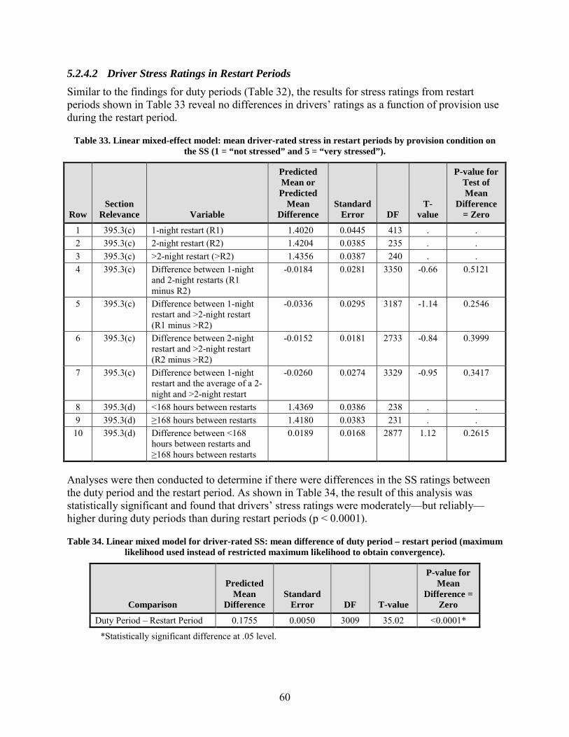
60

5.2.4.2 Driver Stress Ratings in Restart Periods Similar to the findings for duty periods (Table 32), the results for stress ratings from restart periods shown in Table 33 reveal no differences in drivers’ ratings as a function of provision use during the restart period.

Table 33. Linear mixed-effect model: mean driver-rated stress in restart periods by provision condition on the SS (1 = “not stressed” and 5 = “very stressed”).

Row



Mean Difference

Standard Error DF

T-value


Difference = Zero



-0.0184 0.0281 3350 -0.66 0.5121


-0.0336 0.0295 3187 -1.14 0.2546


-0.0152 0.0181 2733 -0.84 0.3999


-0.0260 0.0274 3329 -0.95 0.3417



0.0189 0.0168 2877 1.12 0.2615

Analyses were then conducted to determine if there were differences in the SS ratings between the duty period and the restart period. As shown in Table 34, the result of this analysis was statistically significant and found that drivers’ stress ratings were moderately—but reliably—higher during duty periods than during restart periods (p < 0.0001).

Table 34. Linear mixed model for driver-rated SS: mean difference of duty period – restart period (maximum likelihood used instead of restricted maximum likelihood to obtain convergence).

Comparison

Predicted Mean

Difference Standard

Error DF T-value

P-value for Mean

Difference = Zero

Duty Period – Restart Period 0.1755 0.0050 3009 35.02 <0.0001*


61

5.2.4.3 Sleep Duration in Duty Periods Table 35 displays the means and analyses for sleep per 24 hours during duty periods. It is noteworthy that across all provisions, mean sleep was approximately 6.5 hours during the duty period. The analyses did not find statistically significant differences in the use of the provisions during duty periods.

Table 35. Linear mixed-effect model: mean hours of sleep per 24 hours in duty periods by provision condition.

Row



Mean Difference

Standard Error DF

T-value


Difference = Zero



-0.1036 0.0590 2374 -1.76 0.0793


-0.1063 0.0630 2388 -1.69 0.0918


-0.0027 0.0404 2377 -0.07 0.9472


-0.1050 0.0576 2382 -1.82 0.0686



-0.0269 0.0370 2358 -0.73 0.4671

5.2.4.4 Sleep Duration in Restart Periods Table 36 shows drivers’ mean hours of sleep per 24 hours during the restart periods. As shown, Section 395.3(c) affected sleep duration during restarts. The analysis of sleep duration per 24 hours did not find statistically significant differences between 1- and 2-night restarts. However, sleep duration per 24 hours was longer during 1-night restarts compared to more-than-2-night restarts (p < 0.0001), and longer than during the average of the 2-night restart and the more-than-2-night restart (p = 0.01). The 2-night restart averaged higher sleep durations than the more-than-2-night restart (p < 0.0001), because the more nights drivers had for restart, the lower the sleep amount per 24 hours (an indication of dissipating sleep debt across nights of recovery). In addition, Section 395.3(d) was related to sleep duration per 24 hours during restart. When restart occurred at or after 168 hours, sleep duration per 24 hours was longer (p = 0.0457). This pattern was consistent with the reduction of sleep pressure when recovering from a cumulative sleep

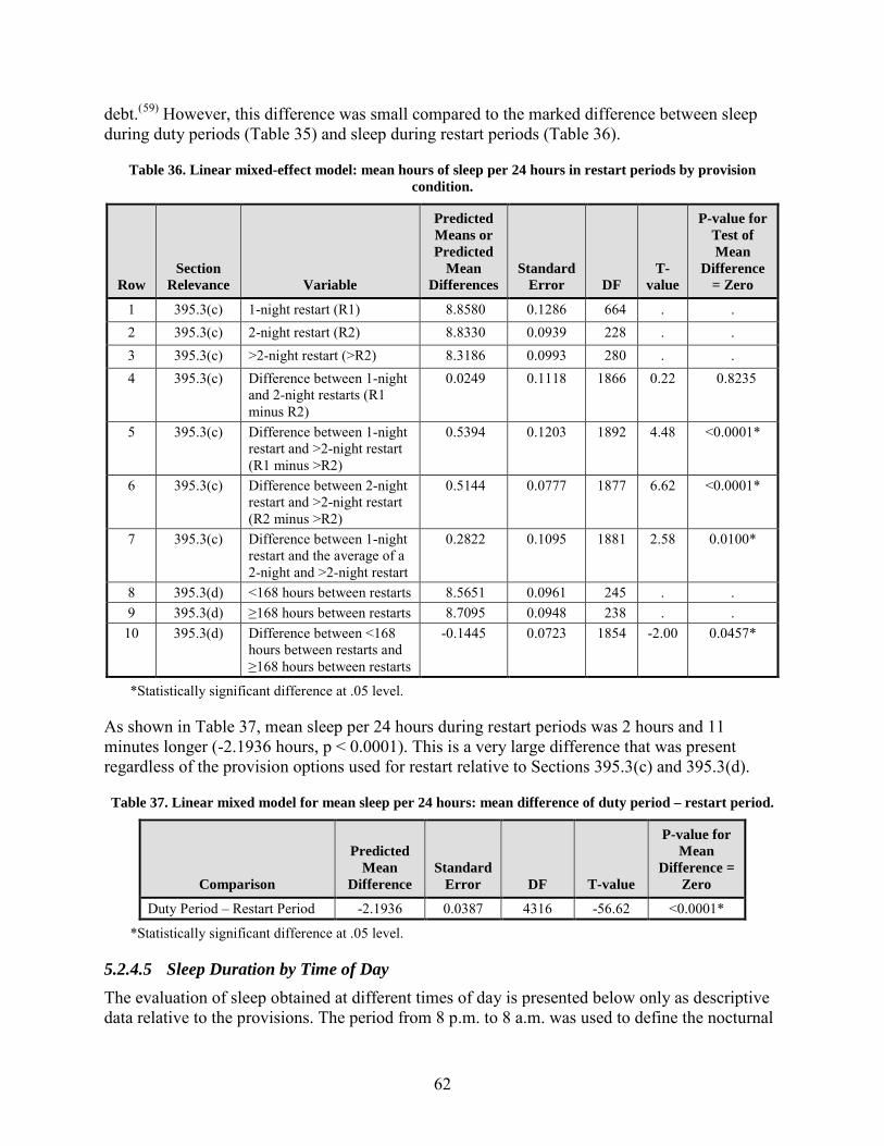
62

debt.(59) However, this difference was small compared to the marked difference between sleep during duty periods (Table 35) and sleep during restart periods (Table 36).

Table 36. Linear mixed-effect model: mean hours of sleep per 24 hours in restart periods by provision condition.

Row


Predicted Means or Predicted

Mean Differences

Standard Error DF

T-value


Difference = Zero



0.0249 0.1118 1866 0.22 0.8235


0.5394 0.1203 1892 4.48 <0.0001*


0.5144 0.0777 1877 6.62 <0.0001*


0.2822 0.1095 1881 2.58 0.0100*



-0.1445 0.0723 1854 -2.00 0.0457*


As shown in Table 37, mean sleep per 24 hours during restart periods was 2 hours and 11 minutes longer (-2.1936 hours, p < 0.0001). This is a very large difference that was present regardless of the provision options used for restart relative to Sections 395.3(c) and 395.3(d).

Table 37. Linear mixed model for mean sleep per 24 hours: mean difference of duty period – restart period.

Comparison

Predicted Mean

Difference Standard

Error DF T-value

P-value for Mean

Difference = Zero



5.2.4.5 Sleep Duration by Time of Day The evaluation of sleep obtained at different times of day is presented below only as descriptive data relative to the provisions. The period from 8 p.m. to 8 a.m. was used to define the nocturnal

63

portion of the day, which is the phase when humans are biologically programmed to sleep. The amount of time drivers were sleeping during this 12-hour phase was then calculated as a percentage of their total time sleeping, to obtain an unadjusted estimate of the extent to which the use of different provision options resulted in sleep that was appropriately timed to the biological phase for sleep.

Sleep timing relative to Section 395.3(c) During their duty periods, drivers who used a 1-night restart obtained approximately 56 percent of their duty sleep during the nocturnal period from 8 p.m. to 8 a.m. The comparable percentages for drivers who had a 2-night or more-than-2-night restart were 78 percent and 84 percent, respectively, during their duty periods. During restart periods, drivers who used a 1-night restart obtained 71 percent of their sleep between 8 p.m. and 8 a.m., compared to 83 percent and 88 percent for drivers who used a 2-night restart and a more-than-2-night restart, respectively. This suggests that drivers who opt for 1-night restarts were more likely to obtain sleep during the diurnal portion of the day than drivers who elected to restart with 2 or more nights of sleep.

Sleep timing relative to Section 395.3(d) During their duty periods, drivers who used a restart in less than 168 hours obtained approximately 75 percent of their duty sleep during the nocturnal period from 8 p.m. to 8 a.m. Those who took a restart after 168 hours or more had approximately 79 percent of their duty sleep during this nocturnal window. During restarts, those who took a restart in less than 168 hours had 82 percent of their restart sleep during the nocturnal period from 8 p.m. to 8 a.m., and those who took a restart at or after 168 hours had 84 percent of their restart sleep in this nocturnal window.

Overall, sleep during the nocturnal portion of the day was more likely during restart periods than during duty periods. Among restart options, 1-night restarts were associated with the lowest proportion of time sleeping during the nocturnal time (8 p.m. – 8 a.m.), when the body is biologically programmed to sleep.

5.2.4.6 Sleep Quality in Duty Periods Drivers provided subjective quality ratings for their sleep periods. The predicted means and analyses of these data are shown in Table 38. The use of the provisions had no relationship to drivers’ sleep quality ratings during duty periods.

64

Table 38. Linear mixed-effect model: mean driver-rated sleep quality ratings in duty periods by provision (1= poor sleep quality, 5=highest sleep quality).

Row



Mean Difference

Standard Error DF

T-value


Difference = Zero



-0.0331 0.0247 2602 -1.34 0.1797


-0.0416 0.0262 2608 -1.59 0.1122


-0.0085 0.0166 2600 -0.52 0.6066


-0.0374 0.0240 2606 -1.55 0.1204



-0.0123 0.0152 2591 -0.81 0.4181

5.2.4.7 Sleep Quality in Restart Periods Table 39 shows drivers’ sleep quality ratings. Sleep quality ratings were associated with provision use during restarts for Section 395.3(c). Sleep quality ratings were lower during a 1-night restart relative to a 2-night restart (p = 0.0114), relative to a more-than-2-night restart (p = 0.0080), and relative to the average of the 2-night restart and the more-than-2-night restart (p = 0.0061). Restart options in Section 395.3(d) had no relationship to sleep quality.

65

Table 39. Linear mixed-effect model: mean driver-rated sleep quality ratings in restart periods by provision (1= poor sleep quality, 5=highest sleep quality).

Row



Mean Difference

Standard Error DF

T-value


Difference = Zero


and 2-night restarts (R1 – R2) -0.0745 0.0294 2585 -2.53 0.0114*

5 395.3(c) Difference between 1-night restart and >2-night restart (R1 - >R2)

-0.0830 0.0313 2596 -2.65 0.0080*

6 395.3(c) Difference between 2-night restart and >2-night restart (R2 - >R2)

-0.0085 0.0198 2589 -0.43 0.6688


-0.0787 0.0287 2591 -2.74 0.0061*



0.0017 0.0182 2576 0.09 0.9262


As shown in Table 40, sleep quality ratings were significantly lower during duty periods than during restart periods (p < 0.0001).

Table 40. Linear mixed model for mean sleep quality rating: mean difference of duty period – restart period.

Comparison

Predicted Mean

Difference Standard

Error DF T-value

P-value for Mean

Difference = Zero

Duty Period – Restart Period -0.0851 0.0108 5336 -7.86 <0.0001


5.3 RESULTS OF WITHIN-DRIVER ANALYSES FOR EFFECTS OF PROVISIONS

In addition to the mixed-model analyses, the research team capitalized on the fact that a substantial number of drivers opted to use 1-night and 2-night restarts, and/or to take restarts in less than 168 hours or in at least 168 hours. This provided another opportunity to conduct simple within-subjects analyses (parametric and nonparametric) to determine the effects of the restart

66

provisions on the study outcomes. Table 41, Table 42, and Table 43 display these within-subjects comparisons. The direction of the comparison can be seen by which percentage is larger, the positive or the negative. The sign-test is very robust and does not depend on any distribution for its validity. This is the primary test for the within-subjects analyses (it is non-parametric). If the paired t-test results are very different than the sign-test results, the sign-test should be interpreted. However, comparisons with a marginal sign-test coupled with a significant paired t-test should be interpreted.

Table 41 displays results for Section 395.3(d). It confirms the mixed-model results that PVT-B lapses in restarts were more frequent during restart periods when restarts were taken in at least 168 hours as compared to less than 168 hours (p = 0.026), and that mean sleep duration in restarts was higher during restart periods when they were taken in at least 168 hours as compared to less than 168 hours (p = 0.0006).

Table 42 provides within-driver results relevant to Section 395.3(c) for a 1-night versus 2-night restart. It confirms the mixed-model results that during the restart period, drivers rated their sleep quality higher during a 2-night restart than during a 1-night restart (p = 0.047). There is also a finding that drivers’ ratings of stress during the restart period were higher during the 2-night restart than during the 1-night restart (p = 0.007).

Table 43 displays the within-subjects comparisons for a 1-night restart compared to a 2-night or more-than-2-night restart. It confirms there was greater driving time with a 1-night restart (p = 0.042) and longer PVT-B response speed (p = 0.046) in restarts during a 1-night restart compared to a more-than-2-night restart. There were fewer PVT-B lapses (p = 0.036) during restarts, drivers rated their difficulty of driver lower (p = 0.014), and drivers’ ratings of stress during restarts were lower (p = 0.003) during a 1-night restart compared to a more-than-2-night restart.

To summarize, the within-subjects analyses provide a different approach to analyzing the data where the data are limited to only drivers that experienced both provisions. This is a powerful statistical approach as it controls for individual error variance because the same drivers are included in both provisional options. The results from these analyses confirm some of the key results of the full mixed-model analyses presented earlier. Therefore, two different approaches to analyze the data were conducted and the results from each approach were similar.

67

Table 41. Within-driver differences for restart <168 hours since last restart minus restart ≥168 hours since last restart.

Outcome Pairs Number positive

Percent positive

Number negative

Percent negative

Number zeros

Mean Difference

Standard Deviation Min Max

Sign Test p-value

Paired T

p-value

Driving Hours per Day 201 92 45.8 109 54.2 0 -0.170 1.098 -7.934 2.266 0.259 0.167 Work Hours per Day 201 90 44.8 111 55.2 0 -0.130 1.325 -11.197 4.707 0.158 0.167 SCE Rate per 100 Hours 201 81 40.3 85 42.3 35 -0.059 5.279 -17.739 51.433 0.816 0.875 PVT-B Mean 1/RT in NR(t) 193 99 51.3 94 48.7 0 0.014 0.183 -1.329 1.126 0.774 0.273 PVT-B Mean 1/RT in R(t) 191 107 56.0 84 44.0 0 0.026 0.198 -0.906 1.016 0.111 0.070 PVT-B Total Lapses in NR(t) 193 93 48.2 100 51.8 0 -0.271 1.948 -12.091 6.080 0.666 0.055 PVT-B Total Lapses in R(t) 191 84 44.0 107 56.0 1 -0.400 2.471 -15.292 6.682 0.111 0.026* Difficulty of Drive 192 92 47.9 83 43.2 17 0.001 0.259 -2.092 1.006 0.546 0.978 Safety Hazards 192 97 50.5 84 43.8 11 -0.007 0.289 -2.738 0.501 0.373 0.721 Stress Scale in NR(t) 193 98 50.8 84 43.5 11 -0.008 0.245 -1.219 1.493 0.335 0.640 Stress Scale in R(t) 191 82 42.9 85 44.5 24 0.012 0.361 -2.463 2.683 0.877 0.649 Fatigue Scale in NR(t) 193 100 51.8 88 45.6 5 0.008 0.223 -0.708 1.442 0.423 0.604 Fatigue Scale in R(t) 191 90 47.1 95 49.7 6 -0.015 0.293 -1.800 0.618 0.769 0.472 KSS Sleepiness in NR(t) 193 97 50.3 95 49.2 1 -0.004 0.399 -2.727 1.722 0.943 0.893 KSS Sleepiness in R(t) 191 88 46.1 102 53.4 1 -0.073 0.545 -3.667 1.118 0.346 0.065 Mean Sleep Quality in NR(t) 175 82 46.9 84 48.0 9 -0.001 0.188 -0.677 0.571 0.938 0.920 Mean Sleep Quality in R(t) 174 83 47.7 76 43.7 15 0.003 0.309 -1.115 2.000 0.634 0.891 Mean Sleep in NR(t) 166 93 56.0 73 44.0 0 0.017 0.612 -1.895 2.553 0.140 0.727 Mean Sleep in R(t) 146 52 35.6 94 64.4 0 -0.184 1.291 -5.189 7.221 0.0006* 0.087

*Statistically significant difference at .05 level. NR(t) = Duty Period; R(t) = Restart Period

68

Table 42. Within-driver differences for 1-night restarts minus 2-night restarts.


Percent positive

Number negative

Percent negative

Number zeros

Mean Difference


Sign Test p-value

Paired T

p-value

Driving Hours per Day 129 73 56.6 56 43.4 0 0.178 1.252 -3.012 5.057 0.159 0.108 Work Hours per Day 129 68 52.7 61 47.3 0 0.198 1.635 -6.570 4.911 0.598 0.171 SCE Rate per 100 Hours 129 43 33.3 56 43.4 30 -0.672 6.059 -51.598 16.387 0.228 0.210 PVT-B Mean Reciprocal RT in NR(t) 120 61 50.8 59 49.2 0 0.021 0.271 -0.779 1.565 0.927 0.408 PVT-B Mean Reciprocal RT in R(t) 118 63 53.4 55 46.6 0 0.029 0.335 -1.059 1.675 0.520 0.351 PVT-B Total Lapses in NR(t) 120 58 48.3 62 51.7 0 -0.229 3.218 -15.009 8.433 0.784 0.436 PVT-B Total Lapses in R(t) 118 49 41.5 68 57.6 1 -0.264 4.521 -15.444 16.729 0.096 0.527 Difficulty of Drive 120 45 37.5 62 51.6 13 -0.010 0.305 -0.864 1.203 0.122 0.733 Safety Hazards 120 54 45.0 57 47.5 9 -0.032 0.371 -1.099 1.190 0.850 0.347 Stress Scale in NR(t) 120 50 41.7 62 51.9 8 -0.025 0.383 -1.194 1.634 0.299 0.475 Stress Scale in R(t) 118 37 31.4 65 55.1 16 -0.020 0.385 -1.250 1.909 0.007* 0.574 Fatigue Scale in NR(t) 120 61 50.8 59 49.2 0 0.010 0.285 -0.841 1.063 0.927 0.649 Fatigue Scale in R(t) 118 52 44.1 57 48.3 9 0.019 0.400 -1.083 1.600 0.702 0.613 KSS in NR(t) 120 54 45.0 65 54.2 1 -0.019 0.491 -2.015 1.583 0.359 0.675 KSS in R(t) 118 57 48.3 59 50.0 2 -0.033 0.627 -2.711 2.148 0.926 0.564 Mean Sleep Quality in NR(t) 109 44 40.4 55 50.5 10 -0.061 0.358 -1.486 1.003 0.315 0.080 Mean Sleep Quality in R(t) 108 44 40.7 50 46.3 14 -0.099 0.516 -2.438 2.222 0.606 0.047* Mean Sleep in NR(t) 104 45 43.3 59 56.7 0 -0.115 0.812 -2.285 2.903 0.202 0.151 Mean Sleep in R(t) 92 48 52.2 44 47.8 0 -0.030 1.774 -7.170 3.783 0.755 0.874


69

Table 43. Within-driver differences for 1-night restart minus 2-night and more-than-2-night restarts.


Percent positive

Number negative

Percent negative

Number zeros

Mean Difference


Sign Test p-value

Paired T

p-value

Driving Hours per Day 132 75 56.8 57 43.2 0 0.225 1.2621 -2.973 5.577 0.139 0.042* Work Hours per Day 132 75 56.8 57 43.2 0 0.233 1.4592 -5.218 5.637 0.139 0.069 SCE Rate per 100 Hours 132 41 31.1 66 50.0 24 -0.174 3.5825 -12.573 18.362 0.020 0.578 PVT-B Mean Reciprocal RT in NR(t) 123 60 48.8 63 51.2 0 0.024 0.2395 -0.674 1.280 0.857 0.260 PVT-B Mean Reciprocal RT in R(t) 123 73 59.4 50 40.7 0 0.054 0.3166 -0.835 1.435 0.046* 0.062 PVT-B Total Lapses in NR(t) 123 60 48.8 63 51.2 0 -0.302 2.9256 -15.009 6.196 0.857 0.255 PVT-B Total Lapses in R(t) 123 49 39.8 73 59.4 1 -0.442 4.2184 -18.333 12.952 0.036* 0.247 Difficulty of Drive 123 43 35.0 70 56.9 10 -0.005 0.2831 -0.750 1.087 0.014* 0.831 Safety Hazards 123 55 44.7 61 49.6 7 -0.029 0.3426 -1.055 1.146 0.643 0.355 Stress Scale in NR(t) 123 52 42.3 65 52.9 6 -0.013 0.3590 -1.215 1.658 0.267 0.691 Stress in R(t) 123 39 31.7 70 56.9 14 -0.016 0.3609 -1.439 1.274 0.003* 0.633 Fatigue Scale in NR(t) 123 64 52.0 59 48.0 0 0.012 0.2842 -1.125 0.832 0.719 0.649 Fatigue Scale in R(t) 123 61 49.5 61 49.5 1 0.008 0.4165 -1.363 1.474 1.000 0.822 KSS in NR(t) 123 57 46.3 66 53.7 0 -0.009 0.4406 -1.460 1.620 0.471 0.820 KSS in R(t) 123 62 50.4 59 48.0 2 -0.056 0.6713 -2.674 2.684 0.856 0.353 Mean Sleep Quality in NR(t) 111 49 44.1 57 51.4 5 -0.059 0.3568 -1.486 1.091 0.497 0.085 Mean Sleep Quality in R(t) 110 47 42.7 54 49.1 9 -0.107 0.4917 -1.936 2.289 0.551 0.025* Mean Sleep in NR(t) 107 49 45.8 58 54.2 0 -0.053 0.8390 -2.339 3.330 0.439 0.514 Mean Sleep in R(t) 95 52 54.7 43 45.3 0 0.102 1.6983 -5.041 3.986 0.412 0.560


70

5.4 POOLABILITY ANALYSES FOR THE EFFECTS OF PROVISIONS

As stated in the statute, “The study shall include fleets of all sizes (i.e., small, medium, and large) and operations (including long-haul, regional, and short-haul) in various sectors of the industry (including flat-bed, refrigerated, tank, and dry-van) to the extent practicable. Thus, a third set of analyses were conducted as part of this study. Although the study was not powered to compare outcome differences associated with the two provisions as a function of type of operation or fleet size, the study plan indicated these differences would be assessed in descriptive “poolability” analyses using appropriate summary statistics. The sampling plan required representativeness of industry elements diverse in company size, type of operation, and industry sector. This forms the basis for the poolability analysis to evaluate whether restart provision effects were consistent across subsets of the trucking operations represented in the study. Specific contrasts are statistically pooled over fleet sizes in order to compare among types of operations. In general, the focus of comparisons across sampling strata was to evaluate whether it can be confidently concluded that results (relative to restart schedules) compare across drivers from different fleet sizes and different types of operations.

Tables 45–80 in Appendix L present the results of the poolability analyses. The takeaway message from the poolability analyses is that the results show that diversity in the industry, relative to carrier size, operations, and industry sector, does not differ in the use of the provisions and their effects on different outcome domains. A notable exception is found in Table 75 on sleep time during restarts. Drivers from large carriers (estimate = 0.5133) and regional carriers (estimate = 0.6862, p = 0.0006) appear to get less sleep during 2-night restarts than during 1-night restarts, but the opposite is the case for medium carriers (estimate = -0.4757, p = 0.0158) and small carriers (estimate = -0.8713, p = 0.0042). This is evidence of a qualitative interaction between industry segment and provision use.

Another interesting observation is found in Table 69, which displays the results for the duration of restart as determined through ELD data. Not surprisingly, all segments indicate a longer restart when drivers take a 2-night restart relative to a 1-night restart. However, the difference in the length of the restart appears to be two- to three-fold across segments, with shorter restarts occurring in small companies, in tanker operations, and in long-haul operations. In contrast, longer restarts occurred in large companies, short-haul operations, and flatbed trailers.

It is recognized that some of the differences in the poolability analyses are due to chance, given the number of comparisons. The tables should be used to look for large qualitative interactions, such as in Table 69 and Table 75, where one segment is significantly negative while another is significantly positive. These poolability analyses were designed to add detail concerning the possibility of variations in the overall outcomes by segment. Other analyses of the data and future studies will be necessary to shed further light on how diversity of trucking operations affects the utility and impact of the restart provisions.

71

6. CONCLUSIONS, LIMITATIONS, AND FUTURE CONSIDERATIONS

6.1 SUMMARY OF RESULTS OF THE EFFECT OF SECTION 395.3(C) ON OUTCOMES

The mixed-effects model results presented in Tables 12–40 indicate that the use of the 1-night restart option versus the 2-night restart option in Section 395.3(c) had effects on some of the study outcomes, as did Section 395.3(d). However, the magnitude of the effects was modest compared to the overall benefit afforded by a restart. The results of this extensive naturalistic investigation of how CMV operators use Sections 395.3(c) and 395.3(d) of Title 49, Code of Federal Regulations, relative to operational, safety, fatigue, and health outcomes revealed both expected and unexpected findings in the four outcome domains.

6.1.1 Operational Outcomes Drivers’ mean driving hours per 24 hours in duty periods were as follows: 8.22 hours for drivers using a 1-night restart, 8.08 hours for drivers using a 2-night restart, and 8.00 hours for driver using a more-than-2-night restart. The mean driving hours per 24 hours in duty periods for drivers using the 1-night restart were significantly greater than they were for drivers using the more-than-2-night restart (t-value = 2.37, p = 0.018). Mean driving hours per 24 hours in duty periods were the same (8.06 hours) for drivers who had less than 168 hours between their restart periods and for drivers who had at least 168 hours between their restart periods.

Drivers’ mean work hours per 24 hours in duty periods were as follows: 10.20 hours for drivers using a 1-night restart, 10.11 hours for drivers using a 2-night restart, and 9.98 hours for drivers using a more-than-2-night restart. Mean work hours per 24 hours in duty periods following a 1-night restart were significantly greater than mean work hours per 24 hours in duty periods following a more-than-2-night restart (t-value = 2.30, p = 0.021). Mean work hours per 24 hours in duty periods following a 2-night restart were also significantly greater than mean work hours per 24 hours in duty periods following a more-than-2-night restart (t-value = 2.14, p = 0.033). For drivers with less than 168 hours between restart periods, mean work hours per 24 hours in duty periods were 10.11; for drivers with at least 168 hours between restart periods, mean work hours per 24 hours in duty periods were 10.03.

6.1.2 Safety Outcomes The primary safety outcomes were the rates of SCEs and fatigue-related SCEs per 100 hours instrumented driving time captured via OBMS. These included electronically-recorded hard braking, hard acceleration, swerves, contact with other objects, and driving in excess of posted speed limits. As shown in Table 16, the rates of SCEs per 100 hours instrumented driving time in duty periods were as follows: 0.34 for drivers using a 1-night restart, 0.37 for drivers using a 2-night restart, and 0.35 for drivers using a more-than-2-night restart. For drivers with less than 168 hours between restart periods, the rate of SCEs per 100 hours instrumented driving time in duty periods was 0.36; for drivers with at least 168 hours between restart periods, the rate was 0.37.

72

The rates of fatigue-related SCEs per 100 hours instrumented driving time in duty periods were as follows: 0.00 for drivers using a 1-night restart, 0.01 for drivers using a 2-night restart, and 0.00 for drivers using a more-than-2-night restart. For drivers with less than 168 hours between restart periods and for drivers with at least 168 hours between restart periods, the rate of fatigue-related SCEs per 100 hours instrumented driving time in duty periods was 0.00.

6.1.3 Fatigue Outcomes Driver fatigue was objectively assessed by measuring driver alertness performance on daily iterations of an electronic PVT-B performance test, and subjectively assessed via driver ratings of fatigue and sleepiness. Driver ratings of fatigue were higher during 1-night restarts (p = 0.0371), but not during duty periods following 1-night restarts. In both restart and duty periods, PVT-B response speed was slowest in drivers who took restarts that were longer than 2 nights. Relative to Section 395.3(d), PVT-B response speed was slower and PVT-B lapses were more frequent when drivers restarted at 168 hours or more compared to less than 168 hours. This was the case for PVT-B performance in both duty periods and restart periods (p values between 0.0503 and 0.0087, Tables 18, 19, 22, 23, and 24). This suggests that restarts taken after 168 or more hours reduce psychomotor vigilance performance due to cumulative fatigue. Consistent with this finding was the fact that drivers averaged more sleep during restarts that occurred in 168 hours or more than they did during restarts that occurred in less than 168 hours (p = 0.0457, Table 36).

Other evidence that drivers were consistently fatigued by the time they took restarts, regardless of the provision used, derives from comparisons of drivers’ responses during duty periods compared to their responses during restarts. In addition to slower PVT-B responses (p < 0.0001, Table 20) during restart periods compared to duty periods, drivers had a higher rate of PVT-B lapses of attention (p < 0.0001, Table 25); higher sleepiness ratings (p < 0.0001, Table 28); and higher fatigue ratings (p < 0.0001, Table 31) during restarts than during duty periods. Consistent with this evidence of behavioral fatigue is the fact that drivers averaged more than a 2-hour increase in sleep duration during restart compared to duty periods, regardless of the provision they used to restart.

Drivers averaged a statistically-predicted mean of greater than 8.5 hours of sleep per 24 hours during restarts of 1 or 2 nights and regardless of the 168-hour rule used. This is approximately 30 percent more sleep than they routinely obtained each day during duty periods (p < 0.0001, Table 37). Their statistically-predicted mean sleep time on duty days was less than 6.6 hours per 24 hours, which is below the recommended 7-hour threshold for daily sleep to promote health (as recently published by the American Academy of Sleep Medicine and the Sleep Research Society).(60,61,62) Collectively, the data suggest that drivers developed a cumulative sleep debt during duty periods, which increased their biological sleep propensity (i.e., the tendency to fall asleep and sleep longer) during restarts. This outcome would be consistent with drivers also reporting more subjective fatigue and sleepiness, and manifesting reduced PVT-B performance during restarts as compared to duty periods. There is little known scientifically about the potential effects of repeated cycling through sleep restriction and sleep extension. Although this study suggests the sleep restriction-recovery differential is large (and common in the trucking industry), the health and performance effects of repeated cycling through sleep restriction need to be better understood in this cohort.

73

6.1.4 Health Outcomes The value of restarts for increasing needed sleep time in drivers was evident in the results, but there also was evidence that restart sleep was perceived as better by the drivers. Drivers rated restart sleep to be of higher quality than sleep during duty periods (p < 0.0001, Table 40). Both adequate sleep duration and sleep quality are essential aspects of sleep health. It is noteworthy that relative to Section 395.3(c), drivers rated 2-night restarts to be of higher sleep quality than 1-night restarts (p < 0.0114, Table 39). The provisions did not affect drivers’ ratings of stress, but drivers rated their stress higher during duty periods than during restart periods (p < 0.0001, Table 34). Therefore, restart periods served to mitigate driver fatigue, sleep loss and stress.

6.2 RESULTS RELATIVE TO FEDERAL SECTIONS 395.3(C) AND 395.3(D)

The use of 1-night and 2-night restarts, as well as more-than-2-night restarts, was expected, as was the additional sleep time the restart afforded drivers for recovery from work fatigue and reduced sleep time when working. The limited number of effects on duty periods from the type of restart used for each provision was unexpected. For example, sleep time was not different between the restart provisions during duty periods. On the other hand, drivers’ fatigue ratings were higher during 1-night restarts relative to 2-night and more-than-2-night restarts (statistically reliable differences). Drivers’ ratings of sleep quality during 1-night restarts were lower than during 2-night and more-than-2-night restarts (statistically reliable differences).

6.2.1 1-Night Restarts and Restarts Taken in 168 Hours or More The slightly elevated subjective fatigue during 1-night restarts [Section 395.3(c)], and the slightly decreased PVT-B performance during both restart and duty periods associated with restarts greater than or equal to 168 hours [Section 393.5(d)], are consistent with an elevated sleep drive when these provisions are used. This was also evident in the fact that drivers obtained more sleep per 24 hours during the 1-night restart compared to the more-than-2-night restart (p < 0.0001), and more sleep when restarting at or after 168 hours than before 168 hours (p = 0.0457). Thus it appears that greater fatigue induced by these two options in the provisions is mitigated in part by somewhat greater sleep amounts during restart (Table 36).

Although of modest size, these reliable differences were found even when 1-night restarts were compared to the average of all restarts greater than 1 night. This suggests that relative to Section 395.3(c), restarts of 2 or more nights may result in subjectively better quality sleep and less fatigue relative to 1-night restarts. On the other hand, these modest subjective differences in the restart periods had no relationship to fatigue ratings and PVT-B performance during duty periods, which did not vary by how Section 395.3(c) was used.

The results also suggest that restarting when reaching 168 hours or more [Section 395.3(d)] resulted in greater subjective and objective indicators of fatigue. Thus, relative to Section 395.3(d), restarting in less than 168 hours was associated with faster PVT-B response times and fewer PVT-B lapses of attention during both restart periods and subsequent duty periods (again, these were modest but statistically reliable differences). Sleep duration per 24 hours was also longer when the restart was taken at or after 168 hours. These findings suggest that drivers

74

experienced modest but reliable decreases in behavioral alertness for restarts that occurred at or after 168 hours [Section 395.3(d)].

Collectively, the data suggest that greater fatigue can be expected when drivers utilize the 1-night restart and take a restart in 168 hours or more. It is possible that a restart period of extended sleep can compensate for the cumulative sleep loss (sleep debt) from repeated duty days of reduced sleep. However, the long-term health and/or performance consequences of this pattern are not clear. There is a need to determine how to reduce some of the cumulative sleep debt of drivers by increasing duty day sleep time. Even small increments of 20–30 minutes per day may be beneficial for health and performance.

6.3 CONCLUSIONS

What was evident in the study results was the markedly increased sleep time afforded by the restarts relative to sleep during work weeks. Sleep time per 24 hours was increased by more than 2 hours from duty time amounts. This kind of differential between sleep duration when working and sleep duration when off duty also has been found in three studies(63,64,65) over the past 10 years (see Appendix A) that have used actigraphy to track sleep in CMV operators during duty periods and restart or off-duty periods—although the present data set is by far the largest collected on this topic. The consistency of the finding that sleep during duty periods is markedly less than sleep on off-duty days (including restarts) in CMV operators should not be ignored relative to the provisions or to future studies. There is extensive scientific evidence that inadequate sleep is a risk factor for many common health conditions (e.g., obesity, diabetes, and hypertension) as well as errors and accidents. As noted above, a recent comprehensive consensus report from the American Academy of Sleep Medicine and the Sleep Research Society by a group of scientists who used a modified RAND Appropriateness Method to conclude that “insufficient sleep” involves sleeping less than 7 hours per day. The CMV drivers who participated in this study average below that level on their working days.

The studies of sleep in CMV drivers, including the extensive data in this study, indicate that drivers obtain 6–6.5 hours of sleep a day for 4–7 days straight (i.e., up to 168-hour limit), before getting an opportunity to sleep long enough to recover from a sleep debt. There is a need to identify ways to increase the amount of time drivers spend sleeping within the 10 consecutive hours of off-duty time required by the current HOS regulations and avoid the risk that repeated chronic partial sleep loss poses to the health and safety of commercial truck drivers.

This study provided clear evidence that drivers were in need of sleep when they undertook a restart, and when they slept, it was much longer than when they slept on work/duty days. They were more fatigued; sleepier; less behaviorally alert on the PVT-B performance test; and less stressed during restarts than on duty days. Regardless of the restart provision used [Section 395.3(c) or Section 395.3(d)], there was evidence that the restart benefitted the ability of drivers to get some recovery from work stress, cumulative fatigue, and chronic sleep restriction. The drivers who participated in the study have made an important contribution to a continued evidenced-based approach to safe operations by CMV drivers.

75

6.4 STUDY LIMITATIONS

There are strengths and limitations of any research approach. The following is a description of the study’s limitations.

6.4.1 Naturalistic Study Methodology The Act directed FMCSA to conduct a CMV Driver Restart Study. Congress directed that within 90 days of enactment of The Act, “the Secretary shall initiate a naturalistic study of the operational, safety, health, and fatigue impacts of the restart provisions in Sections 395.3(c) and 395.3(d) of Title 49, Code of Federal Regulations, on commercial motor vehicle drivers.” A naturalistic study of human behavior requires researchers to carefully observe and record behavior over a period of time in a natural setting, without applying an intervention, and while minimizing interference with the participants being monitored. This describes precisely how the CMV Driver Restart Study was conducted. It was fully observational without interventions or randomization of participants to different procedures. During the course of their participation, drivers directed their own schedules.

This approach limits the ability to determine the exact cause of a behavior (e.g., why a given restart provision was used by a CMV driver) and it prevents the control or measurement of variables that may influence behavior. Also, like other research methods, naturalistic studies can result in participants changing their behavior in a manner they think is desired by the researchers (i.e., demand characteristics), rather than behaving the way they normally would. These studies may also result in people changing behaviors by virtue of their awareness that they are being monitored. Finally, naturalistic studies may have a higher number of volunteer participants who feel they can tolerate the monitoring. They may differ in unknown ways from those who do not want to be monitored in a study, and therefore do not volunteer.

These factors may have been present in the study in varying degrees, but every effort was made to provide no guidance to participants as to how they conducted their work-rest activities and schedules. They were assured that their data was treated with strict confidentiality, and the only information provided to them was in relation to study compensation and use of study equipment.

6.4.2 Technology Use The study used low-burden, minimally-obtrusive wrist actigraphy and smartphone app technologies to record drivers’ sleep timing, duration, and quality. Physiological assessment of drivers’ sleep using polysomnography would have provided a more precise measure of sleep timing, duration, and continuity, but it was beyond the scope, practicality, and cost of the study, and just as importantly, it would have risked altering the naturalistic study design by requiring the repeated application of electrodes for sleep recordings. In contrast, wrist actigraphy and electronic self-report of sleep times and quality are minimally intrusive, cost-effective, and demonstrated to provide reasonably good estimates of physiological sleep time and sleep quality. Therefore, these technologies were used in the study.

6.4.3 Fatigue Coding of Onboard Monitoring System Data The method of determining driver fatigue from the OBMS data was to review the OBMS clips to look for, and score, overt fatigue by using procedures used in previous naturalistic driving

76

studies. The technology vendor in this study used an 8-second pre-trigger duration, which was likely insufficient to reliably determine a driver’s level of fatigue. However, it is unlikely that this limitation impacted the conclusions regarding fatigue, as the primary fatigue measure was the PVT-B test.

6.4.4 Seasonal Variance Data acquisition for the study occurred from March through September in the northern hemisphere. Data were not acquired in the winter, when driving can pose greater weather-related risks. Driver participants came from across the United States, which further contributed to the representativeness of the study data. However, it is possible that had the study monitored driving in the winter, the drivers may have used the provisions in different ways.

6.4.5 Driver Data Self-report Drivers were asked to provide their height and weight, as well as whether they had been diagnosed as having certain disorders (e.g., high blood pressure), and whether they were prescribed medications/therapies for those disorders. Self-report of such information is less reliable than physical measurements and confidential medical evaluations, which would have been beyond the scope of this naturalistic study. Consequently, the information that drivers provided regarding their physical and medical status may have limited accuracy.

6.5 OPPORTUNITIES FOR FUTURE RESEARCH

The analyses conducted in this study were focused on addressing the research questions that were directed in the statute. However, an important by-product of this study is a very rich data set that can be mined to answer many additional research questions that were not addressed in this report. This data set will provide the research community with a new opportunity to inform techniques and strategies that can be used to better the safety, health, and wellness of CMV drivers and the motoring public. This public-use dataset will provide the opportunity to further the science regarding work schedules and fatigue. Potential studies include examining fatigue of drivers working and driving for extended hours; fatigue levels of drivers who sleep less than 5 hours per 24-hour period; modeling the relationship between amount of sleep and off-duty time; examining how fatigue varies across the work day and work week; examining the impacts of driving breaks; and potentially modeling the aspects of driver schedules that are associated with greater fatigue.

77

APPENDIX A: LITERATURE REVIEW The published literature was reviewed for recent information pertinent to the issue of CMV driver fatigue and recovery times needed between work weeks, with a focus on four areas:

1. New studies on the need for recovery from fatigue and the effectiveness of the 34-hour restart.

2. Significant findings from domestic and international research relating to commercial vehicle driver fatigue.

3. Significant findings from the military, Federal Aviation Administration, transit industry, and Federal Railroad Administration (regulations for training railroad engineers) on the effectiveness and measurable safety benefits of an adequate recovery period.

4. Health outcomes and sleep among CMV drivers.

STUDIES ON THE NEED FOR RECOVERY FROM FATIGUE AND THE EFFECTIVENESS OF THE 34-HOUR RESTART

Crash Risk, Breaks, and 34-hour Restart In addition to addressing the number of hours that a CMV driver may drive and be on duty, the HOS regulations set the minimum amount of time that must be reserved for rest, which includes behaviors that promote recovery and the ability to work again. These behavioral requirements include time not working in the form of breaks during work, and time away from work to recover from acute and chronic work fatigue. Additional support for the benefits of breaks has recently been reported. Increases in crash risk for driving up to 11 hours have been found, but crash odds were incrementally reduced by one and two breaks in the latter half of a 10- to 11-hour drive in truckload (TL) and less-than-truckload (LTL) drivers.(66,67)

This work also revealed that drivers who had 34 hours or more off-duty (i.e., a 34-hour restart) immediately prior to a driving period had a nearly 43 percent increase in crash odds, which diminished on subsequent work days. The reasons for this risk elevation following the 34-hour restart are unknown, including whether they are associated with drowsy driving. One recent CMV naturalistic study found approximately 30 percent of all observed instances of drowsiness occurred within the first hour of the work shift, and observed instances of drowsiness were twice as likely to occur between 6 a.m. and 9 a.m., as compared to baseline or non-drowsy driving.(68) A database study of falling-asleep crashes (all vehicles) in North Carolina also found that they peaked in frequency between 6 a.m. and 9 a.m.(69) These are the hours of the day when sleepiness can be elevated from no sleep the night before,(70) from multiple days of sleep restriction,(71,72) and/or from sleep inertia.(73)

The range of possible contributors to CMV driver drowsiness serves to emphasize the importance in determining whether any of the following factors contribute to driver fatigue and crash risk immediately after a 34-hour restart:

78

• Time of day of the first drive after restart.

• Duration of restart recovery sleep.

• Quality of restart recovery sleep.

• Continuous time awake prior to restart first drive.

• Time of day of sleep during restart.

• Extent to which non-driving work occurred prior to the first drive post-restart. (74)

• Drivers’ perceptions of stress following the 34-hour restart. (75)

• Perceived difficulty of the drive.

• Perceived degree of drive hazards.

• Driver characteristics that have been found to be associated with elevated crash risk (e. g., younger age, high blood pressure).

• Prior exposure of drivers to a Fatigue Management Program (FMP).

Although the current driver restart study does not have sufficient data to evaluate crash risk per se, data has been acquired on factors that may contribute to driver safety and fatigue after 34-hour restarts, relative to Sections 395.3(c) and 395.3(d) of Title 49, Code of Federal Regulations (CFR). These measures include SCEs, which are relevant to crash risk,(76) as well as work time, drive time, sleep-wake timing on work days and restart days, fatigue, sleepiness, stress, driver-reported age, and a variety of self-reported health conditions. These data were acquired across a representative group of trucking operations.

Drivers’ Sleep on Workdays Versus Sleep on Off-duty Days An issue central to the 34-hour restart provision is the promotion of adequate recovery from CMV driver fatigue by providing the “circadian advantages of nighttime sleep,”(77) which is defined in the regulation as two consecutive sleep opportunities during biological and environmental nights (operationalized as 1 a.m. to 5 a.m.). Thus, the 34-hour restart provision was intended to provide drivers an opportunity to obtain two 8-hour rest periods to promote recovery from cumulative sleep deprivation (i.e., sleep debt).(78) In addition, over the past 10 years there have been a number of naturalistic studies in which CMV drivers wore wrist actigraph devices to objectively record their sleep periods (onset/offset times) and sleep duration per 24 hours. Table 44 displays the results of three of these naturalistic studies, including the 2014 field study of the 34-hour restart provision.(79,80 ,81)

These studies (and others) confirm that the amount of sleep per 24 hours obtained by CMV drivers on workdays is consistently less than the amount of sleep per 24 hours obtained on non-workdays (gray background on Table 44), suggesting that drivers accumulate a sleep debt and attempt to pay it off by sleeping longer during restarts and days off. This response is consistent with laboratory evidence of the fatiguing effects of restricting sleep to less than 7 hours of time in bed per day for 1 week(82,83) and evidence of a compensatory increase in sleep duration for 1 or more nights being essential to help recover performance and alertness deficits following 5 days of sleep restriction.(84) The mean differences in Table 44 between sleep per 24 hours on

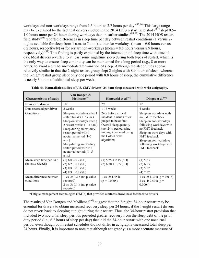
79

workdays and non-workdays range from 1.3 hours to 2.7 hours per day.(85,86) This large range may be explained by the fact that drivers studied in the 2014 HOS restart field study(87) slept 0.5–1.0 hours more per 24 hours during workdays than in earlier studies.(88,89) The 2014 HOS restart field study(90) reported differences in sleep time per day between restart conditions (1 versus 2-nights available for sleep from 1 a.m. to 5 a.m.), either for workdays (mean = 6.0 hours versus 6.2 hours, respectively) or for restart non-workdays (mean = 8.8 hours versus 8.9 hours, respectively).(91) This finding is partly explained by the interaction of sleep time with time of day. Most drivers reverted to at least some nighttime sleep during both types of restart, which is the only way to ensure sleep continuity can be maintained for a long period (e.g., 8 or more hours) to avoid a circadian-mediated termination of sleep. Although the sleep times appear relatively similar in that the 2-night restart group slept 2-nights with 8.9 hours of sleep, whereas the 1-night restart group slept only one period with 8.8 hours of sleep, the cumulative difference is nearly 3 hours of additional sleep per week.

Table 44. Naturalistic studies of U.S. CMV drivers’ 24-hour sleep measured with wrist actigraphy.

Characteristics of study Van Dongen &

Mollicone(92) Hanowski et al.(93) Dinges et al.(94)

Number of drivers 106 29 12 Data recorded per driver 2 weeks 1-16 weeks 4 weeks Conditions Sleep on workdays after 1

restart break (1–5 a.m.) Sleep on workdays after ≥ 2 restart breaks (1–5 a.m.) Sleep during an off-duty restart period with 1 nocturnal period (1–5 a.m.) Sleep during an off-duty restart period with ≥ 2 nocturnal periods (1–5 a.m.)

24 h before critical incident in which truck judged to be at fault Overall sleep quantity (per 24-h period using midnight centered using the Cole-Kripke algorithm)

Sleep on workdays with no FMT* feedback Sleep on non-workdays following workdays with no FMT feedback Sleep on work days with FMT feedback Sleep on non-workdays following workdays with FMT feedback

Mean sleep time per 24 h (hours ± SD/SE)

(1) 6.0 ± 0.2 (SE) (2) 6.2 ± 0.1 (SE) (3) 8.8 ± 0.3 (SE) (4) 8.9 ± 0.2 (SE)

(1) 5.25 ± 2.15 (SD) (2) 6.70 ± 1.65 (SD)

(1) 5.23 (2) 6.53 (3) 5.02 (4) 7.52

Mean difference between conditions

1 vs. 2: 0.2 h (no p-value reported) 2 vs. 3: 0.1 h (no p-value reported)

1 vs. 2: 1.45 h (p = 0.0005)

1 vs. 2: 1.30 h (p = 0.018) 3 vs. 4: 2.50 h (p = 0.0004)

*Fatigue management technologies (FMTs) that provided alertness/drowsiness feedback to drivers

The results of Van Dongen and Mollicone(95) suggest that the 2-night, 34-hour restart may be essential for drivers to obtain increased recovery sleep per 24 hours, if the 1-night restart drivers do not revert back to sleeping at night during their restart. Thus, the 34-hour restart provision that included two nocturnal sleep periods provided greater recovery from the sleep debt of the prior duty period (i.e., 6.2 hours of sleep per day) than did the 34-hour restart with one nocturnal period, even though both restart schedules did not differ in actigraphy-measured total sleep per 24 hours. Finally, it is important to note that although actigraphy is a more accurate measure of

80

sleep duration than self-reports of sleep duration,(96) like the latter, it tends to overestimate physiological sleep time.(97)

FINDINGS FROM DOMESTIC AND INTERNATIONAL RESEARCH RELATING TO COMMERCIAL VEHICLE DRIVER FATIGUE AND TECHNOLOGIES TO MANAGE FATIGUE

Human Factors and Ways to Reduce Fatigue-Related CMV Crashes The Canadian Council of Motor Transport Administrators (CCMTA) completed a major report in 2011 entitled “Addressing Human Factors in the Motor Carrier Industry in Canada.”(98) The report found that numerous sources and methodologies indicate the most significant causation factors for CMV crashes relate to drivers’ recognition (caused either by fatigue [hypovigilance] or distraction) and decision errors, rather than performance errors or the use of drugs and alcohol. This resulted in a set of 44 action items to address fatigue, distraction, and risky driving. Although not mentioned in the CCMTA report, the relationships between fatigue, distraction, and risky behaviors are more intimate than commonly assumed. An extensive naturalistic study of SCEs found that the most frequent critical reasons assigned to CMV drivers for SCEs involved internal distractions (57.1 percent), external distractions (11.4 percent), and drowsiness (8.9 percent).(99) Recent scientific studies have established that sleep loss increases distractibility,(100) which suggests inadequate sleep can be central to driver inattention and distractibility.

The CCMTA report concluded that HOS regulations are necessary but not sufficient to address fatigue in the motor carrier industry.(101) Although HOS rules were regarded as the foundation of fatigue management, the report proposed various initiatives to generate a comprehensive and efficient fatigue management approach endorsed by industry and government. Among the initiatives the report recommended to reduce fatigue-related CMV crashes were the following:

• HOS rules enforced with tamper-proof equipment (e.g., electronic onboard recorders).

• Evaluation of the operational and safety effects of new HOS rules in Canada.

• Study of the psychological determinants of the decision to keep driving while fatigued.

• Study of pay structure as a determinant of the decision to keep driving while drowsy.

• Increased driver training in the causes, consequences, and management of fatigue.

• Adoption of Web-based FMPs by all stakeholders.

• Increased use of scientific evidence on the mitigation of fatigue by recovery sleep.

• Evaluation and implementation of fatigue monitoring technologies.

• Implementation of crash avoidance technologies (e.g., collision warning systems).

• Screening and treatment of obstructive sleep apnea (OSA) in CMV operators.

• Increase understanding of how to optimize rest areas for fatigue mitigation.

81

• Installation of lateral and central rumble strips.

Human Factors and Technologies to Reduce Fatigue-Related Risks in CMV Drivers Inadequate sleep quantity and quality each day are the primary contributors to fatigue and loss of alertness in CMV drivers. Sleep quantity and quality are heavily influenced by sleep environment. Drivers have consistently been observed to sleep longer during restart and when off duty at home, than during work weeks (as shown in Table 44). On the other hand, sleep quality is rarely assessed, even though it is primarily a subjective rating. It is important to assess quality as well, because the reason sleep may be of shorter duration on workdays may relate to disruptions of sleep that reduce the quality, and thus the ability, to sleep. A recent study of Australian truck drivers found that sleep quality was rated as being higher at home than in the truck (p < 0.05). The main obstacles to obtaining good sleep at home were noise and family issues, and the main obstacles to obtaining good sleep when away from home were noise, temperature, and finding a suitable place to stop the truck.(102) The Australian study suggests the domain of technologies for monitoring and mitigating fatigue in CMV drivers should include the sleeping environment during on-duty and off-duty periods.

Since humans are genetically programmed to sleep each day during the nocturnal period, they cannot reverse this biological imperative without accumulating a sleep debt (as shown in Table 44) and suffering cumulative adverse health effects.(103) Maintaining human alertness and behavioral capability under conditions of sleep loss and circadian misalignment requires FMTs to be able to evaluate:

• Dynamic nonlinear modulation of performance capability by the interaction of sleep homeostatic drive and circadian regulation.

• Large differences among people in neurobehavioral vulnerability to sleep loss.

• Error in subjective estimates of fatigue on performance.

• Informing people of the need for recovery sleep.(104)

Therefore, the ability of those who work/drive at night to obtain adequate sleep during duty periods requires optimizing the sleep environment to minimize sleep debt, and optimizing the detection of driver fatigue from sleep debt when working and driving. It has increasingly been noted in recent years that the growing number of cost-effective FMTs can have a key role in minimizing sleep debt and maximizing driver alertness. (See References 105, 106, 107, and 108). Promising areas of technology for managing fatigue risk in safety-sensitive occupations, such as CMV driving, include preventing fatigue by optimizing work-rest schedules using biomathematical models of performance changes associated with sleep homeostatic and circadian dynamics; use of technologies such as the PVT-B as a quick aid for detecting fatigue from sleep loss;(109) and online video or machine-vision tracking of facial signs of sleepiness (e.g., percentage of eye closure [PERCLOS]), which have been validated to be associated with lapses of attention(110) and drowsy driving.(111) However, there have been few systematic evaluations of the extent to which FMTs can improve driver sleep and waking alertness. One notable exception is a naturalistic study in which a variety of FMT approaches were combined. This study revealed that during night driving, FMT feedback significantly reduced drivers’

82

drowsiness (p = 0.004) and lane tracking variability (p = 0.007), and significantly increased driver sleep duration on days off duty by an average of 1 hour (p = 0.018).(112)

FINDINGS FROM THE MILITARY, FEDERAL AVIATION ADMINISTRATION, TRANSIT INDUSTRY, AND FEDERAL RAILROAD ADMINISTRATION (REGULATIONS FOR TRAINING RAILROAD ENGINEERS) ON THE EFFECTIVENESS AND MEASURABLE SAFETY BENEFITS OF AN ADEQUATE RECOVERY PERIOD

Fatigue Management in Commercial Aviation Fatigue management was also a focus of an extensive review of aircrew fatigue, sleep need and circadian rhythmicity, and fatigue countermeasures.(113) The authors concluded that although aviation technology that allows travel over multiple time zones in a single day is a major advance, it poses substantial challenges to sleep and circadian physiology, which can result in flight crew fatigue. Their analysis had many parallels to the fatigue issues faced in commercial trucking. Operational demands resulting in extended work days, increased workload levels, reduced sleep opportunities, and disrupted circadian cycle continue to pose significant challenges during aviation operations. Current prescriptive approaches to fatigue prevention in commercial aviation do not adequately address sleep and circadian challenges associated with operations that run 24 hours per day, 7 days per week, nor do they provide operational flexibility. This has resulted in increasing interest in evidence-based nonprescriptive approaches for the management of fatigue in aviation operations. The authors conclude there is a need to develop approaches that exceed current fatigue management practices by implementation of scientifically valid and operationally feasible technologies that adjust, in real-time, to an individual’s fatigue level and provide an intervention to help manage the fatigue in flight crew members. They assert that, although it may not be possible at this time to know which FMTs will be most useful and acceptable in commercial aviation, it is fairly certain that in order for valid technologies to be used, they must not violate the privacy rights of individuals. It is for this reason they conclude that FMTs in commercial aviation should first be developed as personal aids. They also conclude these technologies must be used responsibly, as they are not a substitute for reasonable working conditions. They anticipate that if these principles are followed, information from FMTs can help people involved in commercial aviation to be less fatigued and more alert, and this is an achievable goal worthy of our best efforts.

Sleep, Fatigue, and Accidents in the U.S. Railroad Industry A recent Federal Railroad Administration report provided a comprehensive description of fatigue in U.S. railroad workers employed in safety-sensitive positions.(114) Five survey studies were conducted between 2006 and 2011 on maintenance-of-way employees, signalmen, dispatchers, train and engine (T&E) employees, and T&E employees engaged in passenger service. These studies were re-analyzed and compared with regard to work schedules and sleep patterns. Fatigue exposure was determined by analysis of work schedules and sleep patterns with a fatigue biomathematical model, the Fatigue Avoidance Scheduling Tool (FAST). Twelve different schedules of work were identified in the five groups of railroad employees. Work schedules largely determined sleep patterns, which, in turn, determined fatigue exposure. T&E crews and dispatchers had the highest fatigue exposure, but these two groups had considerably less fatigue

83

exposure than T&E crews who were involved in accidents. Passenger service T&E employees had the least fatigue exposure, even though the distribution of work time was highly similar to that of T&E employees. This difference in fatigue exposure may be due to the greater predictability of work for the passenger service T&E. The authors found the risk (probability × cost) of an accident caused by human factors increased exponentially with fatigue exposure. The methodology they applied makes it possible to identify differences in sleep patterns as a function of work group and work schedule. They recommend that future work on fatigue in occupational groups should focus on similar methods to expand knowledge of the role of work schedules on sleep, fatigue, and accident risk.

HEALTH OUTCOMES AND SLEEP AMONG CMV DRIVERS

Obesity is a major public health and economic concern due to its promotion of morbidity and mortality. Obesity-related conditions include OSA, heart disease, stroke, type 2 diabetes, and certain types of cancer—some of the leading causes of preventable death. Currently, 34.9 percent (78.6 million) of U.S. adults are obese.(115) A recent Centers for Disease Control and Prevention (CDC) obesity prevalence study by occupation of 37,626 employed Washington State respondents found that truck drivers had the highest prevalence of obesity (38.6 percent) among 28 occupations.(116)

A new study utilized 88,246 commercial driver medical examinations from 2004–13 to estimate the prevalence of obesity, comorbidities, and certification outcomes.(117) A majority of the drivers were obese (53.3 percent, BMI > 30.0 kg/m2), and many were morbidly obese (26.6 percent, BMI > 35.0 kg/m2), which was found to be higher than prior reports. Obese drivers were less likely to be certified for 2 years and more likely to report heart disease, hypertension, diabetes mellitus, nervous disorders, sleep disorders, and chronic low back pain (all p < 0.0001). There were relationships between multiple potentially disqualifying conditions and increasing obesity (p < 0.0001). Morbid obesity prevalence increased 8.9 percent and prevalence of three or more conditions increased fourfold between 2005 and 2012. The authors concluded that obesity is related to multiple medical factors as well as increasing numbers of conditions that limit driving certification.(118)

These recent studies indicating a high prevalence of obesity and associated health risks in CMV drivers have implications for driver fatigue and alertness. It has been well established that obesity is the cause of OSA in the vast majority of adults, and that if left untreated or under-treated, sleep apnea leads to excessive daytime sleepiness in CMV drivers,(119) which has been associated with crash risk.(120) Obesity also has been associated with driver fatigue and SCEs.(121,122) There is also epidemiological evidence that restriction of daily sleep time to less than 6 hours per day results in an increased prevalence risk of obesity, as well as diabetes, hypertension, cardiovascular disease, and all-cause mortality. This raises the possibility that a combination of reduced sleep time during duty periods (as shown in Table 44) and a limited selection of healthy food availability while on the road(123) may promote obesity in drivers, which in turn places them at greater risk for disorders that further limit their ability to cope with sleep debt and operate safely.

84


85

APPENDIX B: BACKGROUND SURVEY

Please answer all questions as accurately as possible. All information is confidential and anonymous.

Boxes should get a checkmark or an “X”. Example: X Blank lines allow you to input your answer as a number or text response.

1. Age? _____years

2. Gender? __ male __ female

3. Married? __ no __ yes

4. What is you height? ___ feet ___ inches

5. What is your weight? ______ pounds

6. Years of driving experience ______ years

7. Years at present company _______ years

8. Type of driver? Day / Night/ Mixed

9. What is your home terminal time zone used for HOS logs _______ (Eastern/Central

Mountain/Pacific)

10. Have you participated in a Fatigue Management Program (FMP)? __ no __ yes __ unsure

11. Has a physician informed you that you have any of the following conditions? (Mark all that apply to you.) __ Sleep apnea __ Diabetes

__ High blood pressure __ Insomnia

12. Do you use any of the following? (Mark all that apply to you) __ CPAP for sleep apnea __ Medication for diabetes __ Medication for high blood pressure __ Medication for insomnia

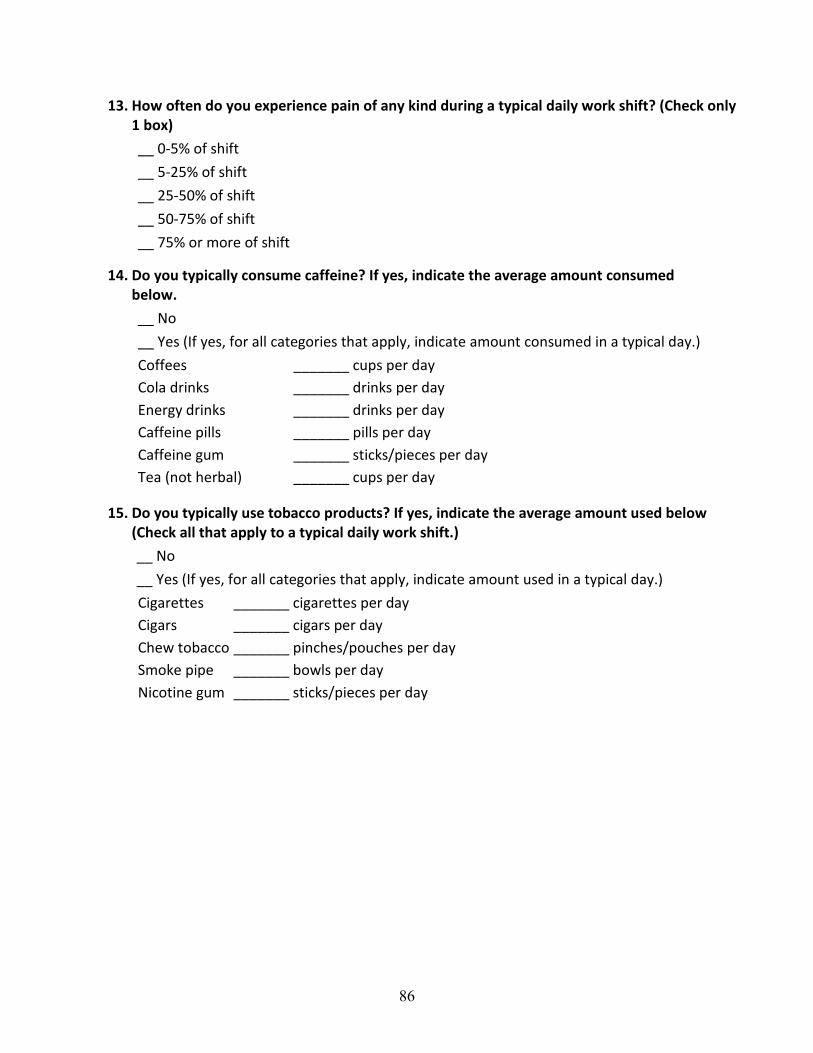
86

13. How often do you experience pain of any kind during a typical daily work shift? (Check only 1 box) __ 0-5% of shift __ 5-25% of shift __ 25-50% of shift __ 50-75% of shift __ 75% or more of shift

14. Do you typically consume caffeine? If yes, indicate the average amount consumed below. __ No __ Yes (If yes, for all categories that apply, indicate amount consumed in a typical day.) Coffees _______ cups per day Cola drinks _______ drinks per day Energy drinks _______ drinks per day Caffeine pills _______ pills per day Caffeine gum _______ sticks/pieces per day Tea (not herbal) _______ cups per day

15. Do you typically use tobacco products? If yes, indicate the average amount used below (Check all that apply to a typical daily work shift.) __ No __ Yes (If yes, for all categories that apply, indicate amount used in a typical day.) Cigarettes _______ cigarettes per day Cigars _______ cigars per day Chew tobacco _______ pinches/pouches per day Smoke pipe _______ bowls per day Nicotine gum _______ sticks/pieces per day

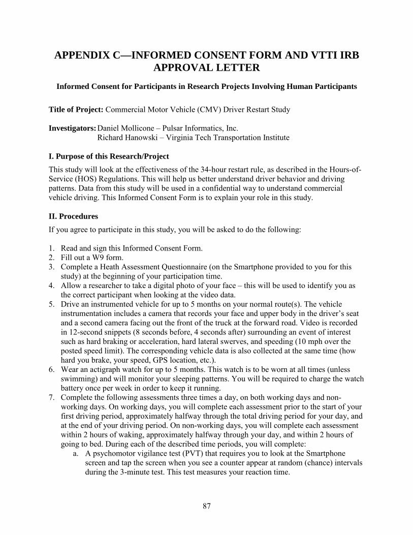
87

APPENDIX C—INFORMED CONSENT FORM AND VTTI IRB APPROVAL LETTER

Informed Consent for Participants in Research Projects Involving Human Participants

Title of Project: Commercial Motor Vehicle (CMV) Driver Restart Study Investigators: Daniel Mollicone – Pulsar Informatics, Inc.

Richard Hanowski – Virginia Tech Transportation Institute I. Purpose of this Research/Project This study will look at the effectiveness of the 34-hour restart rule, as described in the Hours-of-Service (HOS) Regulations. This will help us better understand driver behavior and driving patterns. Data from this study will be used in a confidential way to understand commercial vehicle driving. This Informed Consent Form is to explain your role in this study. II. Procedures If you agree to participate in this study, you will be asked to do the following: 1. Read and sign this Informed Consent Form. 2. Fill out a W9 form. 3. Complete a Heath Assessment Questionnaire (on the Smartphone provided to you for this

study) at the beginning of your participation time. 4. Allow a researcher to take a digital photo of your face – this will be used to identify you as

the correct participant when looking at the video data. 5. Drive an instrumented vehicle for up to 5 months on your normal route(s). The vehicle

instrumentation includes a camera that records your face and upper body in the driver’s seat and a second camera facing out the front of the truck at the forward road. Video is recorded in 12-second snippets (8 seconds before, 4 seconds after) surrounding an event of interest such as hard braking or acceleration, hard lateral swerves, and speeding (10 mph over the posted speed limit). The corresponding vehicle data is also collected at the same time (how hard you brake, your speed, GPS location, etc.).

6. Wear an actigraph watch for up to 5 months. This watch is to be worn at all times (unless swimming) and will monitor your sleeping patterns. You will be required to charge the watch battery once per week in order to keep it running.

7. Complete the following assessments three times a day, on both working days and non-working days. On working days, you will complete each assessment prior to the start of your first driving period, approximately halfway through the total driving period for your day, and at the end of your driving period. On non-working days, you will complete each assessment within 2 hours of waking, approximately halfway through your day, and within 2 hours of going to bed. During each of the described time periods, you will complete:

a. A psychomotor vigilance test (PVT) that requires you to look at the Smartphone screen and tap the screen when you see a counter appear at random (chance) intervals during the 3-minute test. This test measures your reaction time.

88

b. A drowsiness assessment, caffeine diary, stress rating, and a sleep/wake/duty diary on the provided Smartphone.

These assessments will take approximately 30 minutes each day. You will also be required to charge the Smartphone approximately once per day in order to keep it running.

8. Log your hours of service in the BigRoad app on the Smartphone and allow a DashLink adapter to be plugged into your vehicle diagnostic port. You will be required to log your hours of service in the BigRoad app throughout the study period, in addition to logging your hours of service using your company procedures to be compliant with law enforcement.

9. Participate in a brief (approximately 5 – 10 minute) phone call with a researcher, approximately once a week, to review your assessments.

10. Participate in a debriefing phone call at the end of your participation to provide feedback from the study to a member of the research team. You will also receive instructions on how to return the equipment at this time.

For this study we will be collecting data from up to 300 commercial-vehicle drivers like you. The starting day of data collection is determined by the date when you start driving an instrumented vehicle. III. Risks and Discomforts There are some risks and discomforts to which you may be exposed to in volunteering for this research. These risks include: 1. The risk of a crash associated with driving a commercial vehicle as you usually do. 2. The risk of completing the questionnaires is minimal and similar to completing office

paperwork. 3. If you do not already have a Lytx Video Event Recorder (VER) in your vehicle, there may be

stress associated with being recorded while driving if the VER is triggered, for example, due to hard braking, hard acceleration, hard lateral swerve, or speeding. The video will show your face, and a forward view and your actions in response to the driving situation.

4. If you drive into an area where cameras are not allowed, including international border crossings, certain military and intelligence locations, and certain manufacturing facilities, there is a risk that you may be detained or arrested or that your vehicle may be impounded.

5. There is an additional risk not encountered in everyday driving. While you are driving the instrumented vehicle, the VER, if triggered by an event, will record video of you, your actions, and surrounding traffic. In the event of an accident, there is a risk that the video and vehicle parametric data could be obtained in conjunction with a government inquiry or in litigation or dispute resolution. Even if you are not in any accidents, there is a risk of someone outside of the study requesting your data. However, under normal circumstances your identity and the company you work for will be kept confidential.

6. The risk that if the provided Smartphone is lost or stolen, or confiscated by law enforcement or your employer, that these other persons will be able to view your research data and learn your participant number.

7. The risk that your study data may be viewed by people outside of the research team if the Smartphone or actigraph watch is lost in the mail during the return process. However, if

89

either is lost in the mail, there is nothing that ties the data on the Smartphone or actigraph watch to you personally that will be available to whoever finds it.

The following precautions will be taken to ensure minimal risk to the participants:

1. You will be instructed to follow your company’s safety policies. 2. The Smartphone apps you will use during the study will not operate while the vehicle is

moving. 3. Your participation in (or withdrawal from) this study does not have any influence on your

status as an employee with your current company. 4. All data collection equipment will be mounted such that, to the greatest extent possible, it

will not pose a hazard in any foreseeable way. 5. If your provided Smartphone is lost or stolen, we will perform a remote data wipe. 6. In order to help protect the anonymity of your data, it is advised not to include your name

and/or mailing address in any way on, or in, the packaging when returning the equipment at the end of the study. The research team will be tracking which piece of equipment belongs to each driver so there is no need to provide your name with the mailing.

IV. Benefits There are no direct benefits to you for the data collection portion of this study, other than you will have the opportunity to be involved in this very important research study. The results of this study will be briefed to Congress and will be used to modify, as needed, the current CMV HOS regulations. V. Extent of Confidentiality The data gathered in this experiment will be treated with confidentiality. Shortly after participating, your name and the company you work for will be separated from the data and replaced with a number. That is, your data will not be attached to your name, but rather to a number (e.g., Participant 001, Location A). It is possible that the Institutional Review Board (IRB) may view this study’s collected data for auditing purposes. The IRB is responsible for the oversight of the protection of human subjects involved in research. While you are driving the vehicle, a camera will record 12-second snippets (8 seconds before, 4 seconds after) if the VER is triggered because of an event of interest such as hard braking, hard acceleration, hard lateral swerve, or speeding (10 mph over the posted speed limit). Video of your face and out the front of your truck will be recorded during this 12 seconds, as well as audio. An example is shown below. All Lytx data will be encrypted at the time of data collection and will be decrypted only once it arrives back at Lytx and will be stored on a secure server. Access to the video and audio will be limited to Lytx personnel only.

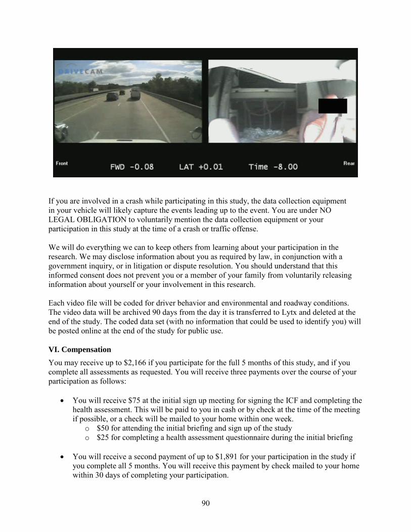
90

If you are involved in a crash while participating in this study, the data collection equipment in your vehicle will likely capture the events leading up to the event. You are under NO LEGAL OBLIGATION to voluntarily mention the data collection equipment or your participation in this study at the time of a crash or traffic offense. We will do everything we can to keep others from learning about your participation in the research. We may disclose information about you as required by law, in conjunction with a government inquiry, or in litigation or dispute resolution. You should understand that this informed consent does not prevent you or a member of your family from voluntarily releasing information about yourself or your involvement in this research. Each video file will be coded for driver behavior and environmental and roadway conditions. The video data will be archived 90 days from the day it is transferred to Lytx and deleted at the end of the study. The coded data set (with no information that could be used to identify you) will be posted online at the end of the study for public use. VI. Compensation You may receive up to $2,166 if you participate for the full 5 months of this study, and if you complete all assessments as requested. You will receive three payments over the course of your participation as follows:

• You will receive $75 at the initial sign up meeting for signing the ICF and completing the health assessment. This will be paid to you in cash or by check at the time of the meeting if possible, or a check will be mailed to your home within one week.

o $50 for attending the initial briefing and sign up of the study o $25 for completing a health assessment questionnaire during the initial briefing

• You will receive a second payment of up to $1,891 for your participation in the study if

you complete all 5 months. You will receive this payment by check mailed to your home within 30 days of completing your participation.

91

o Up to $1,606 for 22 weeks of participation. You will be asked to complete three Smartphone assessments, three times per day and may receive the following payment: $3 per assessment × 3 assessments/day = up to $9/day $9/day × 7 days in a week + $10 bonus for completing all assessments in a

week = up to $73/week 22 weeks × $73/week = $1,606 for completing all assessments

o $25 for participating in a debriefing phone call at the end of the study o $260 bonus for completing all 5 months of participation

• You will receive a third, and final, payment of up to $200 if you return all three pieces of

equipment. Pre-paid packaging materials will be sent to you at the end of the study for you to use to return the actigraph watch, Smartphone, and Lytx system. You will receive this payment by check mailed to your home within 30 days of receiving back the equipment.

o $50 for returning the actigraph watch o $50 for returning the Smartphone o $100 for returning the Lytx system

If you elect to withdraw from the study or if your employment is terminated, you will be compensated for your participation up to that time. You will be asked to return the actigraph watch and Smartphone if you end your participation early. VII. Freedom to Withdraw Participation in this research is voluntary. You are free to withdraw at any time without penalty. If you withdraw, are dismissed from the study, or if your employment is terminated, we will retain data collected before that time, but delete any data collected in the interval between when we become aware of the withdrawal/dismissal and before we are able to remove the data collection equipment. If you withdraw from the study, or if your employment is terminated, you will be paid for your participation up to that time. Withdrawal from this study will not adversely affect your employment status. VIII. Approval of Research This research project has been approved, as required, by the Institutional Review Board for Research Involving Human Participants at Virginia Polytechnic Institute and State University. You should know that this approval has been obtained and is valid for the dates listed at the bottom of this form. IX. Participant's Responsibilities I voluntarily agree to participate in this study. I have the following responsibilities:

1. You will be instructed to follow your company’s safety policies. 2. You will maintain a valid CDL-A throughout the course of the study. 3. To follow the experimental procedures as well as I can. 4. To inform the experimenters if I incur difficulties of any type.

92

X. Participant's Permission I have read and understand the Informed Consent and conditions of this project. I have had all my questions answered. I hereby acknowledge the above and give my voluntary consent for participation in this project. If I participate, I understand that I may withdraw at any time without penalty.

Participant’s name (print) Signature Date

Experimenter’s name (print) Signature Date

Should I have any questions about this research or its conduct, I may contact: Daniel Mollicone, Co-Investigator (206) 673-4733, [email protected] Richard Hanowski, Principal Investigator (540) 231-1513, [email protected] If I should have any questions about the protection of human research participants regarding this study, I may contact: Dr. David Moore, Chair Virginia Tech Institutional Review Board for the Protection of Human Subjects Telephone: (540) 231-4991; Email: [email protected] Participants must be given a complete signed copy (or duplicate original) of the Informed Consent.

mailto:[email protected]



93

VTTI IRB APPROVAL LETTER

95

APPENDIX D—RECRUITMENT POSTER

96


97

APPENDIX E—SCREENSHOTS OF RESTARTSTUDY.COM RECRUITMENT WEBSITE

99

APPENDIX F—FMCSA INDEPENDENT REVIEW PANEL In the regular course of business, FMCSA utilizes an independent peer review when conducting research activities. At the project’s outset, the panel evaluates the clarity of the research questions, the validity of the research methodology, and the quality of the data collection plan. The peer review panel also evaluates the draft final report and comments on the strength of the analyses and the appropriateness of the study conclusions. The Consolidated and Further Continuing Appropriations Act, 2015, required that the initial CMV Driver Restart Study work plan and final report be subject to an independent peer review. The USDOT OIG reviewed the selection of the independent review panel and concluded that “FMCSA selected individuals with relevant medical and scientific expertise.” The peer review panel team members communicated their project reviews and inquiries directly with FMCSA staff.

SELECTION PROCESS AND CRITERIA

FMCSA selected the members of the independent peer review panel based on their scientific and medical expertise. To identify a broad pool of potential team members, FMCSA reached out to the National Academy of Sciences Committee on National Statistics, the American Statistical Association, and several Federal research agencies, such as NIH, for advice on independent experts who could serve on the panel. FMCSA met to review the candidates and narrowed the list to four experts. These individuals represent expertise in statistics, human subject research design, and medical research. FMCSA also gave due consideration to each individual’s independence and ability to objectively review the study, based on a review of their publicly available biographical materials, academic vitae, and résumés. Two of the members are Federal scientists who are required to abide by government-wide ethics and conflict of interest rules. As Federal employees, they do not have ties to industry or other outside groups which could impair their ability to make objective professional judgments regarding the study plan. Two other peer review team members hold academic positions and have experience with national scientific study panels and grant-funded research. A review of their professional backgrounds does not indicate any financial or other ties to industry or other outside groups which could impair their ability to review the study plan and findings objectively. Each of the four peer review panel members came highly recommended by professional colleagues. Each member was required to sign a nondisclosure/conflict of interest statement.

In selecting the peer review panel members, FMCSA followed the overall guidance issued by the OMB Final Information Quality Bulletin for Peer Review (issued December 16, 2004).(124) FMCSA also followed the policies employed by the National Academy of Sciences to ensure independence and avoidance of conflicts of interest. For further information on this topic, see National Academy of Sciences, Policy and Procedures on Committee Composition and Balance and Conflicts of Interest for Committees Used in the Development of Reports, May 2003.(125) The National Academy of Sciences defines conflict of interest as “any financial or other interest that conflicts with the service of an individual on the review panel because it could impair the individual’s objectivity or could create an unfair competitive advantage of a person or organization.”(125)

100

ROLES AND RESPONSIBILITIES

FMCSA provided the peer review team with the project’s draft work plan and methodological design for their review and comment. The team members attended the project kick-off meeting in February 2015 and provided comments to FMCSA. FMCSA evaluated the comments and modified the draft work plan as necessary. Once data collection began, the peer review team was informed of any significant issues that could have changed the research design. FMCSA provided the peer review team with copies of the draft final report for their review and comment.

The Peer Review Charge for this study provided the specific activities assigned to the peer review panel. As recommended by OMB guidelines, FMCSA engaged the peer review team early in the research study process to benefit from their expert review of the research design and methodology.

The peer review panel’s evaluation of the initial study plan included a review of the study hypothesis, soundness of the research methodology, adequacy of the technology used to measure safety performance and driver fatigue, data collection protocol, and analysis plan. The peer review panel also commented on the study’s performance measures to properly evaluate the study outcomes. The independent review of the final report included an evaluation of whether the findings in the report were supportable in view of the statistical evidence provided and whether the report addressed all the items in the initial study plan (see Appendix G and Appendix H).

KEY MILESTONES FOR THE INDEPENDENT PEER REVIEW PANEL

• Peer review panel established – January 2015.

• Peer review panel information submitted to OIG – February 2015.

• Project kick-off – February 2015.

• Peer review panel reviewed study plan prior to submission to OIG – February 2015.

• Peer review panel reviewed draft final report prior to submission to OIG – November 2015.

101

APPENDIX G—PEER REVIEW REPORT SUMMARY: STUDY WORK PLAN AND METHODOLOGY

COMMERCIAL MOTOR VEHICLE (CMV) DRIVER RESTART STUDY: PEER REVIEW OF DRAFT DETAILED WORK PLAN

The present naturalistic study is designed to compare the effects of two commercial motor vehicle (CMV) driver work schedules (restart periods that include 1 versus 2 or more nights) on safety-critical events (SCEs), operator fatigue, and health. The study design is generally solid and reflects the intent of the Congressional directive made through the 2015 Consolidated and Further Continuing Appropriations Act.

PROJECT STRENGTHS:

1. The peer review panel is unanimous in congratulating the FMCSA on its selection of an outstanding research team, which consists of world-renowned experts in fatigue research, naturalistic driving studies, complex field research, and statistics.

2. The use of a mixed “within- and between-subject” design is appropriate and will serve to maximize statistical power.

3. The advanced technology used to capture safety events, sleep, fatigue, and other important variables, coupled with the planned intense follow-up, is likely to result in very high quality data.

4. Although lowering the threshold of the OBMS system to capture potential SCEs is not a perfect solution, it is creative and currently the best way to help ensure that an adequate number of SCEs are captured in a “control/comparison” condition.

PROJECT WEAKNESSES:

1. Given that the primary intent of the study is to examine safety and fatigue in 1-night versus 2-night restarts, sampling to include fleets of all sizes (i.e., small, medium, and large) and operations (including long-haul, regional, and short-haul) in various sectors of the industry for the sake of “generalizability” potentially detracts from the study. The peer review panel recognizes that the researchers’ mandate is to study a “representative” sample. However, from a scientific standpoint, the purpose of ensuring representativeness of a study sample is typically to facilitate the subsequent generalizability of the findings. However, successful generalization requires and pre-supposes (a) that the cells in the sampling plan represent meaningful populations—i.e., populations that might reasonably be expected to be differentially affected by independent variable(s) (in this case, the 1- versus 2-night restart conditions) and (b) that each cell in the sampling plan will have an “n” sufficient to warrant generalization of the study findings. The peer review panel feels that neither of these conditions are satisfied (i.e., that the mandated 36-cell sampling plan is ill-conceived) and worries that expending resources (time and effort) trying to ensure that each of

102

these cells has representation could potentially (and needlessly) impede study efficiency and progress.

2. The original study design did not sufficiently account for driver self-selection effects for choosing a restart condition as well as other potential confounding variables. [This was discussed during the conference call and the investigators indicated that they understood the issues and were making changes to address this weakness. See recommendations below.]

3. It is not clear what will be done during the recruitment phase for a driver who qualifies with respect to the eligibility driving criteria set out on page 14 [of the draft study work plan] (Recruitment and Retention Plan) but who has, for example, a serious health problem. This is an ethical issue, as well as one that bears on the need to be clear about what is meant by generalizability.

4. As indicated previously, the use of smartphone technology to measure subjective fatigue and objective measures of performance is a significant strength. The importance that these devices not be used while driving is clearly understood and adequately addressed. However, it is not clear how the safeguards will impact data collection activities when deployed in team driving situations (i.e., if the device “lockout” while moving will prevent a team driver from entering data while off duty and prior to sleep or awakening in the sleeper berth). To the extent that the study sample includes such driving teams, these issues should be addressed.

Recommendations Given the constraints imposed by the congressionally-directed research mandate, the proposed research plan is generally well-conceived, with appropriately selected dependent variables, appropriate methodology, and a reasonable plan for statistical analyses. Accordingly, although the peer review panel has several suggestions for the research team to consider, we offer only two actual recommendations:

1. There are many unknown confounds that may influence selection of a 1- versus 2-day restart. An effort should be made, for example, using propensity score matching, to balance the two conditions. This requires that more information be collected regarding the reasons for implementing one or the other restart condition. One possibility is to add a survey, perhaps as a smartphone app, that specifies the reason for the type of restart, and the possible reason for using the restart at all. The latter may be particularly helpful for characterizing drivers who take fewer restarts. An additional possibility is to add a question(s) to the background survey regarding the drivers’ attitude[s] toward 1-night restarts in their own schedules.

2. Although generalizability is an important consideration, the current scheme for recruiting drivers does not facilitate the ability to make inferences regarding a more general population. A clear statement of who the target population is and the extent to which the study (recruited) population is representative of that target population should be added.

103

Suggestions: The following are provided only as suggestions for the research team to consider as they conduct the study, analyses, and interpret the findings from this very important study. Accordingly, the research team should feel free to adopt or reject the following suggestions (which are in no particular order) as they see fit:

C. The current subjective measures of fatigue (KSS, FS) do not address the multidimensional nature of fatigue states, such as decreased task engagement, motivation, and the potential relationship between fatigue and broad personality traits such as extroversion and neuroticism. Some research on mood suggests that energetic arousal (or positive affect) is strongly correlated with extroversion and implies that introverts may be particularly prone to fatigue. Viewing fatigue as a complex of unpleasant state symptoms, high neurotic individuals might be more fatigue-prone, given their general tendency towards stress symptoms. This is arguably beyond the scope and intent of the study, but it may be that including broader measures to capture the multidimensional nature of driving-induced fatigue could prove informative, especially if the occurrence of SCEs is low.

D. Broaden the measures of fatigue and stress to capture the multidimensionality of stress and

fatigue states. Consider including trait measures of fatigue. E. Caffeine intake is being measured but not herbal or illicit stimulant use. If anonymity

assurances will ensure accurate reporting, it might be beneficial to collect this information, as well.

F. As a follow-on to the first recommendation re: propensity score matching, it should be noted

that new work has been developed for adaptive treatment studies in randomized trials called SMART designs by Susan Murphy (who just won a MacArthur Award for this work). If each restart period is thought of as an “adaptive treatment assignment” where the “assignment” depends on the driver’s previous “restart-experiences,” appropriate modifications of methods for the analysis of SMART-designed studies may be a useful approach for analysis of this naturalistic study.

G. Potentially meaningful characteristics of the trucking companies, for example, whether or

not they have a fatigue management program (and the quality/comprehensiveness of those programs) is important, and worth capturing.

H. Given that this study is going to occur during the summer months, a statement regarding the

possibility that time-of-year effects could affect the generalizability of the results might be considered (if the researchers agree that this is a possibility).

I. Anticipating that recruitment may not go according to schedule, the panel suggests that a

protocol be specified ahead of time that outlines the steps that would be taken to increase driver recruitment. Having such a plan would add to the transparency of the study, its scientific rigor, and the ability to generalize results.

104

J. As part of the recruitment process, consider collecting information from carriers that quantify the prevalence of drivers in each recruitment category. This information could be used to improve the generalization of the study results to the population of interest, as defined in accordance with recommendation 2.

K. The researchers might consider augmenting the proposed initial data analyses with a few

more exploratory data analyses that as a whole address the impact of self-selecting restart type and other cycle attributes that may confound the effect of the type of restart. For example, the proposed simple analysis might be repeated within groups defined by the reason for selecting the type of restart. Similar simple analyses that incorporate the number of days in each restart/duty cycle and attributes of the previous cycle(s) could potentially differentiate the type of restart from other potential causes of different rates of SCEs such as accumulated fatigue.

L. Similar to suggestions F and K, complex models developed for the final statistical analysis

plan should focus on eliminating confounding due to competing potential causes of different rates of SCEs and other stress and fatigue outcomes.

SUMMARY AND COMMENT

The research team has produced a coherent and comprehensive research study plan that addresses critical questions regarding possible differential effects of restart schedules that include one versus two nighttime periods (during which nighttime sleep is typically obtained). The study is exceptionally well-designed given the constraints imposed by the congressionally-directed sampling requirements, which, in the unanimous opinion of the peer review panel, are inconsistent with the stated goal of facilitating the study’s generalizability. Accordingly, the panel has produced only two recommendations: (a) application of ‘propensity score matching’ to account for self-selection effects that may be attributable to the various reasons for a 1- versus 2-night restart; and (b) a clear explication of the population to which the anticipated results will be generalized. In addition, a number of suggestions for possible modifications or additions to the design and/or analyses were provided by the panel—to be implemented (or not) at the discretion of this exceptional research team.

105

APPENDIX H—PEER REVIEW REPORT SUMMARY: FINAL REPORT

DATE: 25 NOVEMBER 2015

PROJECT SCOPE

The study mandate was to employ a naturalistic field study design to assess the relative effects of the 1- versus 2-night restart options in provision 395.3(c) on operational, performance, safety, health, and fatigue in commercial motor vehicle (CMV) drivers.

Peer Review Methodology The review process implemented for this study—which included teleconferences with key study team members and the peer review panel members at critical junctures in the planning and execution phases of the study—were informative and productive (largely the result of the forethought and care with which these meetings were timed and prepared for by all involved, and the study team’s willingness and ability to rapidly “adjust fire” as necessary). Accordingly, the draft final report contains few surprises, and as detailed below, we (the peer review panel) have only a few remaining questions and suggestions.

Clarity of Hypothesis The study hypotheses were simple and clear: that the effects of the two restart provisions described in Sections 395.3(c) and 395.3(d) of Title 49, Code of Federal Regulations, would differ significantly on outcomes reflecting operational performance, safety, health, and fatigue in commercial motor vehicle (CMV) drivers, with no a-priori hypotheses regarding which restart condition would prove more beneficial. The study team operationally defined each of the outcomes using appropriate and sensitive tests and measures, thus “putting flesh on” what were initially broad and nebulous conceptual requirements.

Validity of Research Design This was a naturalistic field study, subject to all of the limitations inherent to such designs—in particular, the lack of experimental control (e.g., random assignment to 1- versus 2-night restart conditions) that unavoidably limits the ability to determine cause-effect relationships (as pointed out in the report itself, on page 75).

Another criticism of the research design was that, in a well-meaning effort to ensure representativeness of the study sample, there were many irrelevant but mandated “industry segments” (i.e., inclusion of driver categories that were unlikely to systematically impact any of the outcome variables, e.g., drivers of refrigerated trucks, flatbed trucks, panel trucks, etc.). Had the mandated list of driver categories been restricted to those potentially more relevant (e.g., long- versus short-haul) the ability of the study team to recruit for and detect the effects of these potentially more relevant/meaningful industry segments would have been enhanced.

106

Quality of Data Collection Activities

The peer review panel is unanimous in its praise of the study team, who in the draft final report dated November 2015, provide the major findings from a large, complex field study to assess the effects of the restart provisions in Sections 395.3(c) and 395.3(d) of Title 49, Code of Federal Regulations, on the operational, safety, health, and fatigue in commercial motor vehicle (CMV) drivers. By virtue of its scope and size, its nearly flawless execution (no significant protocol deviations), and the alacrity with which the data were analyzed and reported, this study sets a new mark for excellence in naturalistic field studies—a testament to the competence and dedication of the study team.

PEER REVIEW FINDINGS

Robustness and Depth of Analysis Method Used The present data set is massive and the current analyses have only begun to “scratch the surface” of possibilities. It is anticipated that once the data set is made available to the broader research community, it will generate considerable excitement and further, in-depth analyses/exploration.

The study team has adequately conducted all of the required statistical analyses, and ha[s] been receptive to including further analyses requested by the peer review panel. As detailed in the comments by two members of the peer review panel, it was, within the past 2 weeks, suggested that the study team focus the analyses more sharply on the potential bias effects resulting from the differing levels of control that participating drivers exerted over the decision to restart after 1 or 2 nights. (Although this factor was included as a covariate in analyses, more concerted analyses to determine the impact of this factor on the various outcome variables was suggested—a suggestion readily accepted by the study team.) The study team subsequently provided details that satisfied the main concerns of the peer review panel, although presentation of additional analyses to strengthen the conclusions and offset potential selection bias-related criticisms are suggested. As an example, a panel member suggested that the study team might “repeat the presented analyses for subsets related to the probability the particular restart type was experienced” (see below), although several other valid approaches are possible.

Appropriateness of Methods for the Hypothesis Being Tested Within the constraints inherent to naturalistic field studies, the methods were appropriate. The peer review panel was favorably impressed by the study team’s utilization of cutting-edge technology, which helped ensure the currency, accuracy and validity of the data collected over the course of the study.

Extent to which the Conclusions Follow the Analysis In general, and befitting a naturalistic (correlational) field study such as this, the draft final report contains few definitive conclusions regarding the relative benefits of the 1- versus 2-day (or more-than-2 days) restart options on the various outcome measures. Rather, the results of the analyses are mostly “allowed to speak for themselves.”

107

Strengths and Limitations of Overall Product The strengths of the product are considerable, and are generally derived from the obvious care/attention to detail with which the data were collected, and the clarity with which the initial results have been presented in the report.

The limitation of the product generally derive[d] from:

a) The limited ability to infer cause-effect relationships from naturalistic observational studies.

b) The short period of performance afforded to the study team (given another few months, it is likely that the study team would have conducted more extensive exploration and analyses of the data which would have enhanced the richness of the findings included in the report).

c) The mandated inclusion of a large number industry segments – not for scientifically valid or logical reasons (i.e., not because it was expected that these segments would actually account for significant amounts of variance) but to help ensure “representativeness.” This non-scientific requirement unnecessarily added significant logistical (i.e., recruitment-related) burden to the study effort.

d) As detailed in the individual comments of some of the reviewers, it was felt that the organization/presentation of the findings in the draft final report could be improved to enhance clarity and overall impact.

Specific Recommendations for Improvement The peer review panel had relatively few substantive recommendations for improvement: (a) that further analyses be conducted on (and that the final report focus more sharply on) the potential confounds and bias issues surrounding the 1- versus 2-day restart conditions, and (b) that, where possible, more emphasis be placed on within-subject statistical analyses. Remaining recommendations (detailed in the comments of the individual reviewers) focused primarily on (a) enhancing the manner in which the report is organized and the findings are presented; and (b) suggested edits to correct grammatical errors and typos.

SUMMARY OF PEER REVIEW COMMENTS:

Project Strengths: 1. Outstanding study team.

2. Near-flawless study execution/data quality despite severe time pressure.

3. Foresight of the study team reflected in the collection of data on “anticipated restart type” and “reason for anticipated restart type” which permits exploration of possible sources of selection bias.

4. Assessment of the heterogeneity of effects of restart type across diverse industry segments effectively revealed the complexity of this issue.

108

5. Although many additional analyses are possible, the findings that were presented were generally clear, thorough, and directly relevant to the study hypotheses.

Project Weaknesses: 1. Mandated constraints on the study design (i.e., constraints that were beyond the

control of the study team).

2. The report should contain greater detail and/or clarity regarding how, and the extent to which, potential bias or confounding due to self-selection of 1- versus 2-day restart options were dealt with/controlled.

3. Better use of graphs and figures in the report is suggested to facilitate comprehension by non-scientific readers.

4. The ‘recruitment via convenience’ methodology utilized in the present study limits the extent to which the present findings may generalize to the U.S. CMV driver population.

Suggested Improvements: 1. Increased utilization of graphical displays in the report.

2. Inclusion of more analyses to determine the potential effects of self-selection of the 1- versus 2-day restart options.

3. Inclusion of more exploratory data analyses on outcome variables.

4. The report requires proofreading.

109

APPENDIX I—NUMBERS OF INCLUDED AND EXCLUDED SAMPLING UNITS FOR ANALYSIS PER DRIVER

Subject ID Driver has at least 1 SU(t)

Total Number of Sampling

Units Determined

by Algorithm

Total Excluded Sampling

Units

Total Included Sampling

Units

Sampling Units

Excluded from SCE

Analysis Set

Total Sampling

Units Included in

SCE Analysis Set

1 1 9 0 9 0 9 2 1 11 0 11 0 11 3 1 12 0 12 0 12 4 1 1 0 1 0 1 5 1 4 1 3 0 3 6 1 3 0 3 3 0 7 1 9 0 9 0 9 8 1 5 0 5 0 5 9 1 2 0 2 0 2 10 1 9 1 8 0 8 11 1 22 1 21 0 21 12 1 5 0 5 5 0 13 1 10 1 9 0 9 14 1 2 1 1 0 1 15 1 3 0 3 3 0 16 1 9 0 9 0 9 17 1 11 3 8 8 0 18 1 6 0 6 0 6 19 1 11 0 11 6 5 20 1 2 1 1 0 1 21 1 4 0 4 0 4 22 1 5 0 5 5 0 23 1 21 0 21 0 21 24 1 9 0 9 0 9 25 1 22 1 21 0 21 26 1 14 2 12 6 6 27 1 10 1 9 1 8 28 1 8 0 8 0 8 29 1 13 0 13 0 13 30 1 10 0 10 0 10 31 1 3 1 2 0 2 32 1 22 1 21 0 21 33 1 1 0 1 0 1 34 1 14 0 14 11 3 35 1 6 0 6 0 6 36 1 12 0 12 0 12 37 1 21 0 21 1 20

110



Units Determined

by Algorithm


Units


Units

Sampling Units

excluded from SCE

Analysis Set

Total Sampling

Units Included in

SCE Analysis Set

38 1 8 0 8 0 8 39 1 6 0 6 0 6 40 1 13 5 8 0 8 41 1 2 1 1 0 1 42 1 2 0 2 1 1 43 1 7 0 7 0 7 44 1 3 0 3 0 3 45 1 8 0 8 1 7 46 1 6 0 6 0 6 47 1 14 3 11 8 3 48 1 24 1 23 1 22 49 1 21 1 20 0 20 50 1 22 0 22 0 22 51 1 22 1 21 1 20 52 1 17 1 16 0 16 53 1 6 0 6 0 6 54 1 16 2 14 0 14 55 1 20 2 18 0 18 56 1 21 0 21 0 21 57 1 18 7 11 0 11 58 1 2 1 1 1 0 59 1 22 1 21 0 21 60 1 22 1 21 0 21 61 1 24 1 23 1 22 62 1 19 0 19 0 19 63 1 21 0 21 5 16 64 1 23 1 22 0 22 65 1 2 1 1 0 1 66 1 23 1 22 0 22 67 1 22 0 22 0 22 68 1 21 0 21 0 21 69 1 17 1 16 0 16 70 1 22 1 21 0 21 71 1 16 1 15 0 15 72 1 23 1 22 0 22 73 1 5 0 5 0 5 74 1 4 0 4 0 4 75 1 18 1 17 0 17 76 1 18 0 18 0 18 77 1 22 0 22 0 22

111



Units Determined

by Algorithm


Units


Units

Sampling Units

excluded from SCE

Analysis Set

Total Sampling

Units Included in

SCE Analysis Set

78 1 22 0 22 0 22 79 1 24 1 23 2 21 80 1 14 1 13 0 13 81 1 23 1 22 0 22 82 1 23 1 22 0 22 83 1 22 0 22 1 21 84 1 22 1 21 0 21 85 1 22 1 21 0 21 86 1 14 0 14 0 14 87 1 21 0 21 0 21 88 1 18 2 16 3 13 89 1 2 0 2 0 2 90 1 21 5 16 0 16 91 1 4 0 4 0 4 92 1 4 0 4 0 4 93 1 4 0 4 0 4 94 1 12 1 11 0 11 95 1 8 0 8 0 8 96 1 18 3 15 0 15 97 1 21 2 19 6 13 98 1 24 2 22 0 22 99 1 19 0 19 0 19 100 1 10 1 9 0 9 101 1 22 0 22 0 22 102 1 10 1 9 9 0 103 1 12 0 12 1 11 104 1 21 0 21 0 21 105 1 22 3 19 6 13 106 1 4 0 4 0 4 107 1 18 0 18 0 18 108 1 11 0 11 0 11 109 1 8 0 8 0 8 110 1 15 2 13 0 13 111 1 4 0 4 0 4 112 1 19 1 18 0 18 113 1 13 3 10 0 10 114 1 5 2 3 0 3 115 1 6 1 5 0 5 116 1 12 0 12 0 12 117 1 10 1 9 4 5

112



Units Determined

by Algorithm


Units


Units

Sampling Units

excluded from SCE

Analysis Set

Total Sampling

Units Included in

SCE Analysis Set

118 1 2 1 1 0 1 119 1 21 0 21 0 21 120 1 10 1 9 8 1 121 1 29 12 17 4 13 122 1 3 0 3 0 3 123 1 13 5 8 0 8 124 1 21 0 21 0 21 125 1 19 0 19 13 6 126 1 18 3 15 1 14 127 1 27 5 22 5 17 128 1 25 2 23 6 17 129 1 24 2 22 1 21 130 1 10 0 10 2 8 131 1 10 3 7 0 7 132 1 20 0 20 5 15 133 1 25 2 23 0 23 134 1 22 4 18 2 16 135 1 23 3 20 8 12 136 1 3 1 2 0 2 137 1 19 0 19 0 19 138 1 24 3 21 0 21 139 1 3 0 3 0 3 140 1 22 3 19 1 18 141 1 15 3 12 0 12 142 1 19 5 14 0 14 143 1 11 1 10 0 10 144 1 22 7 15 3 12 145 1 13 4 9 0 9 146 1 4 2 2 0 2 147 1 12 0 12 0 12 148 1 22 0 22 15 7 149 1 16 2 14 0 14 150 1 21 3 18 3 15 151 1 11 0 11 6 5 152 1 22 1 21 0 21 153 1 20 3 17 0 17 154 1 17 0 17 0 17 155 1 3 0 3 0 3 156 1 22 5 17 0 17 157 1 15 7 8 0 8

113



Units Determined

by Algorithm


Units


Units

Sampling Units

excluded from SCE

Analysis Set

Total Sampling

Units Included in

SCE Analysis Set

158 1 26 11 15 4 11 159 1 26 4 22 4 18 160 1 20 1 19 0 19 161 1 22 0 22 1 21 162 1 23 2 21 0 21 163 1 17 1 16 3 13 164 1 19 0 19 0 19 165 1 18 1 17 7 10 166 1 19 0 19 0 19 167 1 10 0 10 0 10 168 1 2 0 2 2 0 169 1 26 5 21 0 21 170 1 20 1 19 0 19 171 1 22 0 22 0 22 172 1 21 4 17 5 12 173 1 23 2 21 0 21 174 1 16 0 16 0 16 175 1 23 0 23 1 22 176 1 17 1 16 0 16 177 1 16 4 12 0 12 178 1 4 0 4 0 4 179 1 21 2 19 0 19 180 1 21 0 21 0 21 181 1 22 1 21 0 21 182 1 21 1 20 0 20 183 1 21 1 20 0 20 184 0 1 1 0 0 0 185 1 23 3 20 0 20 186 1 23 3 20 0 20 187 1 22 0 22 0 22 188 1 21 0 21 0 21 189 1 21 1 20 0 20 190 1 20 0 20 0 20 191 1 21 1 20 0 20 192 1 20 0 20 0 20 193 1 19 0 19 0 19 194 1 23 1 22 1 21 195 1 9 1 8 8 0 196 1 5 0 5 0 5 197 1 4 0 4 0 4

114



Units Determined

by Algorithm


Units


Units

Sampling Units

excluded from SCE

Analysis Set

Total Sampling

Units Included in

SCE Analysis Set

198 1 12 2 10 3 7 199 1 21 1 20 0 20 200 1 21 1 20 0 20 201 1 21 2 19 0 19 202 1 15 1 14 0 14 203 1 18 0 18 0 18 204 1 10 0 10 0 10 205 1 11 1 10 0 10 206 1 22 2 20 0 20 207 1 8 2 6 0 6 208 1 12 3 9 5 4 209 1 17 0 17 0 17 210 1 7 2 5 0 5 211 1 19 0 19 0 19 212 1 16 0 16 0 16 213 1 17 0 17 1 16 214 1 21 1 20 0 20 215 1 22 1 21 0 21 216 1 14 1 13 0 13 217 1 16 6 10 0 10 218 1 21 0 21 0 21 219 1 20 1 19 7 12 220 1 10 6 4 0 4 221 1 22 2 20 10 10 222 1 20 0 20 0 20 223 1 30 7 23 7 16 224 1 11 3 8 1 7 225 1 32 8 24 13 11 226 1 23 11 12 2 10 227 1 19 6 13 5 8 228 1 16 0 16 1 15 229 1 21 0 21 0 21 230 1 25 3 22 17 5 231 1 14 2 12 8 4 232 1 18 0 18 0 18 233 1 19 1 18 0 18 234 1 28 5 23 0 23 235 1 4 0 4 0 4 236 1 16 1 15 0 15

Total 235 3,602 315 3,287 299 2,988

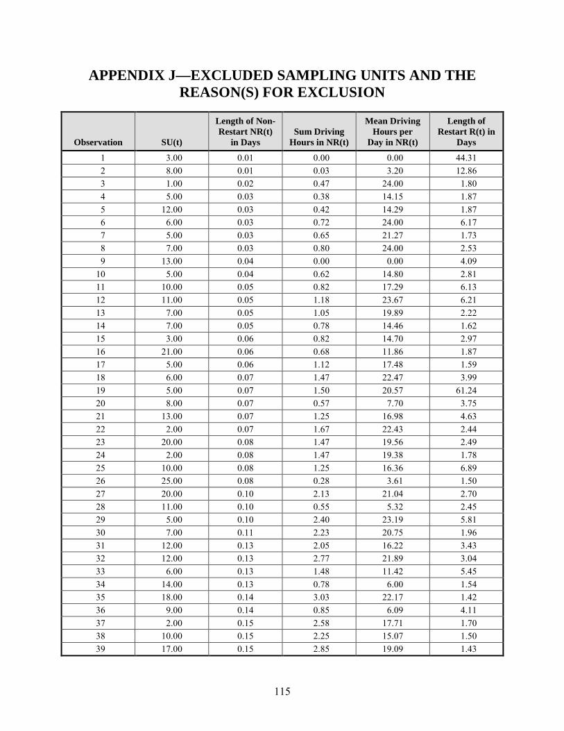
115

APPENDIX J—EXCLUDED SAMPLING UNITS AND THE REASON(S) FOR EXCLUSION

Observation SU(t)

Length of Non-Restart NR(t)

in Days Sum Driving

Hours in NR(t)

Mean Driving Hours per

Day in NR(t)

Length of Restart R(t) in

Days

1 3.00 0.01 0.00 0.00 44.31 2 8.00 0.01 0.03 3.20 12.86 3 1.00 0.02 0.47 24.00 1.80 4 5.00 0.03 0.38 14.15 1.87 5 12.00 0.03 0.42 14.29 1.87 6 6.00 0.03 0.72 24.00 6.17 7 5.00 0.03 0.65 21.27 1.73 8 7.00 0.03 0.80 24.00 2.53 9 13.00 0.04 0.00 0.00 4.09 10 5.00 0.04 0.62 14.80 2.81 11 10.00 0.05 0.82 17.29 6.13 12 11.00 0.05 1.18 23.67 6.21 13 7.00 0.05 1.05 19.89 2.22 14 7.00 0.05 0.78 14.46 1.62 15 3.00 0.06 0.82 14.70 2.97 16 21.00 0.06 0.68 11.86 1.87 17 5.00 0.06 1.12 17.48 1.59 18 6.00 0.07 1.47 22.47 3.99 19 5.00 0.07 1.50 20.57 61.24 20 8.00 0.07 0.57 7.70 3.75 21 13.00 0.07 1.25 16.98 4.63 22 2.00 0.07 1.67 22.43 2.44 23 20.00 0.08 1.47 19.56 2.49 24 2.00 0.08 1.47 19.38 1.78 25 10.00 0.08 1.25 16.36 6.89 26 25.00 0.08 0.28 3.61 1.50 27 20.00 0.10 2.13 21.04 2.70 28 11.00 0.10 0.55 5.32 2.45 29 5.00 0.10 2.40 23.19 5.81 30 7.00 0.11 2.23 20.75 1.96 31 12.00 0.13 2.05 16.22 3.43 32 12.00 0.13 2.77 21.89 3.04 33 6.00 0.13 1.48 11.42 5.45 34 14.00 0.13 0.78 6.00 1.54 35 18.00 0.14 3.03 22.17 1.42 36 9.00 0.14 0.85 6.09 4.11 37 2.00 0.15 2.58 17.71 1.70 38 10.00 0.15 2.25 15.07 1.50 39 17.00 0.15 2.85 19.09 1.43

116

Observation SU(t)


in Days Sum Driving

Hours in NR(t)

Mean Driving Hours per day

in NR(t)


Days

40 1.00 0.15 1.17 7.64 1.83 41 5.00 0.16 3.60 22.94 3.86 42 3.00 0.16 2.62 16.17 2.32 43 14.00 0.17 2.48 14.42 1.83 44 10.00 0.17 2.75 15.90 1.70 45 10.00 0.18 3.77 21.35 1.57 46 12.00 0.18 3.00 16.68 2.00 47 4.00 0.18 0.00 0.00 1.62 48 19.00 0.18 0.45 2.45 1.60 49 7.00 0.19 3.90 20.13 1.67 50 5.00 0.19 4.67 24.00 1.47 51 16.00 0.20 0.93 4.75 2.70 52 15.00 0.20 4.07 20.48 2.14 53 20.00 0.20 1.75 8.78 1.47 54 10.00 0.21 3.50 16.86 1.56 55 12.00 0.21 1.57 7.45 2.20 56 8.00 0.22 2.15 9.77 1.51 57 3.00 0.22 5.35 23.85 4.52 58 14.00 0.23 0.95 4.21 2.51 59 1.00 0.23 5.02 22.16 1.69 60 13.00 0.23 5.02 21.82 1.63 61 8.00 0.24 3.90 16.52 2.29 62 18.00 0.24 5.00 20.99 2.02 63 21.00 0.25 0.00 0.00 1.42 64 1.00 0.25 1.93 7.59 2.02 65 6.00 0.26 4.50 17.42 6.79 66 9.00 0.26 5.95 23.03 4.13 67 14.00 0.26 1.38 5.33 2.34 68 14.00 0.26 5.23 19.94 15.83 69 5.00 0.27 5.42 20.37 1.87 70 4.00 0.27 3.22 12.03 2.68 71 17.00 0.27 6.57 24.00 1.51 72 18.00 0.28 2.18 7.94 3.61 73 15.00 0.28 4.47 16.16 1.96 74 5.00 0.29 4.17 14.53 3.53 75 2.00 0.29 6.43 22.43 1.71 76 13.00 0.29 1.03 3.59 4.63 77 11.00 0.29 1.85 6.30 3.35 78 6.00 0.30 0.63 2.12 6.37 79 1.00 0.30 0.00 0.00 2.93 80 15.00 0.30 4.42 14.55 2.05 81 6.00 0.31 0.37 1.18 1.79 82 17.00 0.31 1.92 6.15 7.68

117

Observation SU(t)


in Days Sum Driving

Hours in NR(t)


in NR(t)


Days

83 15.00 0.31 4.58 14.70 1.68 84 2.00 0.31 1.82 5.81 1.75 85 4.00 0.31 3.37 10.70 1.56 86 1.00 0.31 5.62 17.85 1.45 87 7.00 0.32 5.32 16.72 6.26 88 10.00 0.32 4.25 13.16 1.51 89 20.00 0.32 6.57 20.29 3.13 90 6.00 0.33 5.27 16.21 3.55 91 6.00 0.33 5.02 15.40 5.83 92 1.00 0.33 3.00 9.19 3.57 93 3.00 0.33 3.55 10.88 2.64 94 1.00 0.33 7.33 22.42 1.97 95 14.00 0.33 5.97 18.09 3.44 96 6.00 0.33 0.80 2.40 5.39 97 16.00 0.34 5.67 16.45 2.01 98 12.00 0.35 5.05 14.51 1.85 99 9.00 0.35 1.07 3.05 1.51 100 19.00 0.35 7.62 21.81 6.68 101 18.00 0.35 4.22 12.02 5.19 102 6.00 0.35 2.70 7.67 1.47 103 9.00 0.35 5.85 16.52 6.30 104 12.00 0.36 3.02 8.43 1.55 105 3.00 0.36 7.00 19.57 1.90 106 4.00 0.36 4.25 11.79 3.59 107 15.00 0.36 6.87 18.94 1.86 108 4.00 0.36 4.10 11.29 1.42 109 24.00 0.37 7.13 19.49 2.69 110 4.00 0.38 6.98 18.55 3.40 111 2.00 0.38 5.80 15.27 3.64 112 18.00 0.38 5.65 14.85 1.83 113 5.00 0.38 3.25 8.52 2.69 114 14.00 0.38 4.67 12.24 2.45 115 17.00 0.38 6.77 17.65 1.62 116 11.00 0.39 7.75 20.11 1.68 117 16.00 0.39 3.52 9.11 2.55 118 9.00 0.40 5.70 14.37 1.61 119 2.00 0.40 4.10 10.27 3.58 120 19.00 0.40 6.70 16.69 1.69 121 17.00 0.40 9.05 22.47 1.90 122 20.00 0.40 6.07 15.04 14.55 123 5.00 0.40 6.18 15.33 2.56 124 22.00 0.40 5.52 13.65 2.86 125 3.00 0.40 8.18 20.21 1.46

118

Observation SU(t)


in Days Sum Driving

Hours in NR(t)


in NR(t)


Days

126 15.00 0.41 8.10 19.94 1.52 127 6.00 0.41 7.22 17.55 3.61 128 20.00 0.41 8.23 20.03 1.57 129 9.00 0.41 2.23 5.41 2.41 130 6.00 0.41 7.80 18.85 2.58 131 10.00 0.41 3.12 7.52 2.51 132 18.00 0.41 7.33 17.69 2.49 133 24.00 0.42 6.40 15.33 2.74 134 5.00 0.42 6.50 15.55 2.49 135 21.00 0.42 4.87 11.58 2.59 136 15.00 0.42 7.43 17.66 1.53 137 24.00 0.42 7.90 18.77 3.17 138 14.00 0.42 8.82 20.88 1.70 139 14.00 0.42 8.38 19.82 2.49 140 24.00 0.43 0.57 1.33 1.56 141 16.00 0.43 8.52 19.94 1.69 142 15.00 0.43 2.07 4.81 2.56 143 8.00 0.43 4.25 9.87 3.04 144 12.00 0.43 7.32 16.99 2.60 145 1.00 0.43 8.57 19.80 1.47 146 20.00 0.43 2.97 6.82 1.56 147 5.00 0.43 7.27 16.72 1.52 148 2.00 0.44 7.30 16.74 2.98 149 1.00 0.44 1.90 4.34 1.86 150 14.00 0.44 2.13 4.87 2.58 151 4.00 0.44 6.48 14.77 2.18 152 3.00 0.44 1.37 3.09 2.59 153 7.00 0.44 4.05 9.14 1.52 154 9.00 0.44 8.92 20.13 9.58 155 22.00 0.45 5.73 12.88 2.30 156 4.00 0.45 7.50 16.85 2.51 157 18.00 0.45 8.87 19.89 1.63 158 5.00 0.45 4.83 10.76 4.48 159 27.00 0.45 5.90 13.07 1.50 160 7.00 0.45 6.88 15.25 3.50 161 14.00 0.45 7.85 17.39 5.91 162 10.00 0.45 2.02 4.46 2.55 163 14.00 0.46 0.00 0.00 1.58 164 9.00 0.46 3.62 7.93 3.60 165 8.00 0.46 10.10 22.14 2.04 166 7.00 0.46 4.42 9.61 1.58 167 4.00 0.46 9.22 19.96 1.53 168 12.00 0.46 9.32 20.17 1.68

119

Observation SU(t)


in Days Sum Driving

Hours in NR(t)


in NR(t)


Days

169 6.00 0.46 8.25 17.84 3.60 170 2.00 0.46 9.43 20.40 3.71 171 20.00 0.46 5.70 12.29 1.63 172 9.00 0.46 9.17 19.76 2.58 173 1.00 0.47 1.00 2.14 3.52 174 4.00 0.47 1.18 2.54 1.55 175 18.00 0.47 7.52 16.08 1.50 176 3.00 0.47 9.43 20.09 1.51 177 4.00 0.47 9.68 20.63 1.57 178 12.00 0.47 9.60 20.42 1.52 179 17.00 0.47 9.18 19.45 2.01 180 16.00 0.48 6.05 12.72 4.58 181 7.00 0.48 6.65 13.98 1.53 182 20.00 0.48 6.85 14.40 1.43 183 14.00 0.48 10.45 21.90 12.04 184 15.00 0.48 10.67 22.33 1.62 185 5.00 0.48 7.05 14.69 1.63 186 22.00 0.48 7.95 16.52 2.39 187 8.00 0.49 3.22 6.63 3.33 188 2.00 0.49 6.10 12.48 1.51 189 18.00 0.49 5.58 11.36 2.02 190 6.00 0.49 7.27 14.76 1.51 191 15.00 0.50 3.23 6.53 1.51 192 19.00 0.50 4.73 9.55 2.64 193 7.00 0.50 9.68 19.34 2.42 194 7.00 0.50 8.13 16.22 29.16 195 12.00 0.50 6.62 13.18 2.15 196 25.00 0.51 4.83 9.53 3.23 197 11.00 0.51 10.72 21.14 2.35 198 23.00 0.51 0.93 1.84 1.42 199 3.00 0.51 0.07 0.13 2.51 200 12.00 0.51 6.75 13.17 1.59 201 10.00 0.51 6.22 12.10 1.84 202 1.00 0.51 1.60 3.11 4.51 203 5.00 0.51 3.33 6.48 4.13 204 16.00 0.51 8.52 16.55 1.57 205 1.00 0.52 6.23 12.08 2.00 206 7.00 0.52 5.37 10.39 1.78 207 4.00 0.52 9.62 18.44 1.50 208 10.00 0.53 3.75 7.12 3.70 209 8.00 0.53 5.12 9.67 2.38 210 23.00 0.53 1.87 3.51 2.46 211 11.00 0.54 2.63 4.92 2.82

120

Observation SU(t)


in Days Sum Driving

Hours in NR(t)


in NR(t)


Days

212 2.00 0.54 8.58 15.95 2.51 213 22.00 0.54 4.05 7.52 2.57 214 11.00 0.54 9.90 18.37 1.44 215 4.00 0.54 8.98 16.63 1.48 216 21.00 0.54 9.83 18.11 2.47 217 4.00 0.54 5.70 10.47 80.47 218 4.00 0.54 6.98 12.83 3.06 219 24.00 0.55 8.03 14.74 1.45 220 14.00 0.55 11.00 20.05 2.60 221 3.00 0.55 1.38 2.52 2.55 222 2.00 0.55 9.68 17.52 1.60 223 5.00 0.55 13.13 23.76 9.92 224 1.00 0.55 8.03 14.50 3.22 225 14.00 0.56 9.15 16.43 2.45 226 5.00 0.56 10.60 18.89 2.05 227 12.00 0.56 3.45 6.13 2.35 228 10.00 0.56 4.98 8.83 1.43 229 12.00 0.57 6.03 10.63 2.54 230 11.00 0.57 6.38 11.24 2.43 231 19.00 0.57 11.07 19.39 1.42 232 2.00 0.57 1.42 2.48 1.43 233 1.00 0.57 2.00 3.49 1.52 234 1.00 0.57 2.37 4.13 2.19 235 22.00 0.58 8.67 15.02 1.58 236 12.00 0.58 9.80 16.96 2.03 237 6.00 0.58 10.10 17.48 2.51 238 2.00 0.58 3.45 5.95 2.86 239 15.00 0.58 10.68 18.42 3.58 240 16.00 0.58 9.82 16.87 1.43 241 18.00 0.58 2.28 3.91 1.56 242 8.00 0.58 5.87 10.03 2.05 243 16.00 0.59 9.03 15.41 2.18 244 7.00 0.59 8.97 15.19 3.44 245 22.00 0.59 3.55 5.99 3.44 246 10.00 0.60 9.57 15.98 4.86 247 21.00 0.61 1.35 2.23 1.62 248 1.00 0.61 1.77 2.89 4.47 249 18.00 0.61 6.22 10.16 1.87 250 13.00 0.65 3.30 5.07 2.54 251 7.00 0.65 6.22 9.52 2.31 252 7.00 0.66 12.55 19.08 3.62 253 2.00 0.66 6.00 9.10 2.68 254 7.00 0.67 7.25 10.88 3.15

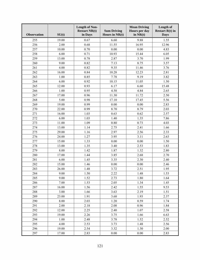
121

Observation SU(t)


in Days Sum Driving

Hours in NR(t)


in NR(t)


Days

255 19.00 0.67 6.60 9.88 1.55 256 2.00 0.68 11.55 16.95 12.96 257 10.00 0.70 0.00 0.00 4.83 258 6.00 0.71 10.93 15.44 6.05 259 13.00 0.78 2.87 3.70 1.99 260 9.00 0.82 7.13 8.75 3.57 261 4.00 0.82 9.35 11.46 3.76 262 16.00 0.84 10.28 12.23 2.81 263 1.00 0.85 7.78 9.19 3.82 264 6.00 0.92 10.15 11.05 1.50 265 12.00 0.93 6.17 6.60 15.48 266 1.00 0.95 4.58 4.84 2.65 267 17.00 0.96 11.30 11.72 2.50 268 5.00 0.98 17.10 17.45 5.56 269 19.00 0.99 0.00 0.00 2.83 270 22.00 0.99 8.70 8.79 2.03 271 16.00 1.03 0.63 0.62 2.57 272 6.00 1.03 1.40 1.35 7.86 273 11.00 1.09 0.80 0.73 4.03 274 13.00 1.14 2.75 2.41 1.66 275 29.00 1.16 2.97 2.56 2.33 276 24.00 1.27 3.95 3.11 2.63 277 15.00 1.33 0.00 0.00 1.50 278 13.00 1.35 3.40 2.53 1.83 279 8.00 1.42 1.87 1.32 2.80 280 17.00 1.44 3.85 2.68 2.70 281 6.00 1.45 3.35 2.30 2.40 282 15.00 1.46 0.00 0.00 2.46 283 26.00 1.48 3.72 2.51 1.95 284 9.00 1.50 2.22 1.48 1.53 285 9.00 1.52 2.73 1.80 1.64 286 7.00 1.53 2.05 1.34 1.45 287 16.00 1.56 2.42 1.55 9.53 288 3.00 1.66 3.63 2.19 1.51 289 23.00 1.91 3.68 1.93 2.37 290 8.00 2.03 1.20 0.59 1.74 291 2.00 2.18 2.08 0.96 1.84 292 12.00 2.25 2.40 1.07 2.58 293 19.00 2.26 3.75 1.66 6.63 294 1.00 2.48 3.78 1.52 2.52 295 4.00 2.53 3.73 1.48 2.56 296 19.00 2.54 3.32 1.30 2.00 297 17.00 2.83 0.00 0.00 2.83

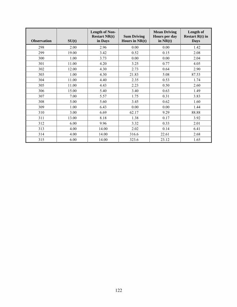
122

Observation SU(t)


in Days Sum Driving

Hours in NR(t)


in NR(t)


Days

298 2.00 2.96 0.00 0.00 1.42 299 19.00 3.42 0.52 0.15 2.08 300 1.00 3.73 0.00 0.00 2.04 301 11.00 4.20 3.25 0.77 4.05 302 12.00 4.30 2.73 0.64 2.90 303 1.00 4.30 21.83 5.08 87.53 304 11.00 4.40 2.35 0.53 1.74 305 11.00 4.43 2.23 0.50 2.60 306 15.00 5.40 3.40 0.63 1.49 307 7.00 5.57 1.75 0.31 3.83 308 5.00 5.60 3.45 0.62 1.60 309 1.00 6.43 0.00 0.00 1.44 310 3.00 6.69 62.17 9.29 88.88 311 13.00 8.18 1.38 0.17 3.92 312 6.00 9.96 3.32 0.33 2.01 313 4.00 14.00 2.02 0.14 6.41 314 4.00 14.00 316.6 22.61 2.68 315 6.00 14.00 323.6 23.12 1.65

123

APPENDIX K—STATISTICAL MODELING METHODS

MIXED-EFFECTS STATISTICAL MODELS

Formal statistical comparisons among expected outcomes on the basis of provision use were performed using linear and non-linear mixed-effects modeling. The objectives of using the mixed modeling approach are:

1. To reduce bias and potential confounding arising from the observational naturalistic study design by producing estimated means and differences in means adjusting for an a priori set of covariates.

2. To adequately account for correlations among outcomes from sampling units from the same driver and among multiple outcomes observed within the same sampling unit. Unless such correlations are adequately accounted for, there can be inflation of type 1 error when testing hypotheses.

The linear mixed-effects model for continuous outcomes(126,127) can be expressed as:

Yi = Xiβ + Ziu + ei

The ‘fixed’ part of this model involves the terms Xiβ. X is a design matrix for the fixed effects. β is the set of parameters to be estimated including provision use factors and the set of covariates. The predicted mean values under each provision condition as well as differences in mean values were estimated as a function of estimates of β. The remaining parts of the model reflect “random effects.” Random effects are used to account for correlations among measurements taken from the same driver and for additional correlations among multiple outcomes measured within the same sampling unit (when applicable). Random effects can be accounted for by the u terms in the above model or by specifying special structure for the covariance matrix of the error terms e. This latter approach is especially applicable for longitudinal data. Generally speaking, the expected values of random effects are equal to zero. This permits all hypotheses of interest to be specified in terms of estimated β’s. The various models for random effects impact on estimated standard errors of model parameters of interest. The random effects used in models are described below. Generalized linear mixed models(128) were used to assess outcomes expressed as counts (PVT-B lapses per 3-minute test) or rates (SCEs).

MODEL COVARIATES

Every model included the following primary factors:

• Number of restart nights (1 night versus 2 nights versus >2 nights)

• Use of the 168-hour provision (<168 hours versus ≥168 hours versus 1st sampling unit). The “1st sampling unit level” for this factor was needed to avoid excluding all first sampling units. This is because classifying sampling units by the 168-hour provision depends on the time between the start of the prior restart period to next restart period, which is unknown for the first sampling unit.

124

• Restart nights by 168-hour provision interaction. The interaction term was included in the model to allow for the effects of one provision on outcomes to vary according to use of the other. However, the focus of estimation was on the main effects of provision use.

Baseline Covariates Every mixed-effects model included an a priori set of covariates that was specified in Table 1 of the study plan. These covariates included both baseline variables and sampling unit specific variables. Restricting attention to an a priori set of covariate reduces bias and helps to control Type 1 error.

There were 2 continuous baseline covariates included in the models. These variables were:

• Driver age.

• Driver BMI.

There were 10 categorical baseline variables. These were:

• Driver in Fatigue Management Program (No, Yes, Unsure).

• Gender (male versus female).

• Marital status (married yes versus no).

• Diabetes (yes versus no).

• High blood pressure (yes versus no).

• Insomnia (yes versus no).

• Sleep apnea (yes versus no).

• Driver pain experience (0–5 percent, 5–25 percent, 25–50 percent, 50–75 percent, ≥75percent). The last two categories were combined in the models due to the small number of drivers reporting ≥75 percent pain.

• Use of caffeine.

• Use of tobacco.

Sampling Unit Specific Covariates In addition to the baseline variables, there were two categorical factors related to driver expectations regarding their next use of the provisions. These factors were obtained from weekly calls made during the non-restart duty cycles.

These 2 factors were:

• For upcoming restart—planned number of nights off? (“Planning 1 Night Next Restart” versus “Planning ≥2 Nights Next Restart” versus “Missing”).

125

• Next restart—night off rationale? (“Largely Due to Federal Regulations” versus “Largely My Company’s Decision” versus “Largely My decision, but Based on Personal Preference” versus “Largely My Decision, but Based on Work Requirements” versus “Missing”).

In cases when there was more than one call prior to a restart, the responses closest to the restart were chosen. In cases when there were no calls prior to a specific restart, a last observation carried forward approach was taken, and the responses from prior restarts closest to the sampling unit in question were used. There was a small percentage of sampling units, often including the first sampling unit, in which there was no prior weekly call. In these cases, the categorical variables were given levels of “Missing” in order to avoid excluding sampling units.

Time-of-Day Models for outcomes collected multiple times per day included a time-of-day factor defined according to home terminal time:

• 12 a.m. to 3:59 a.m.

• 4 a.m. to 7:59 a.m.

• 8 a.m. to 11:59 a.m.

• 12 p.m. to 3:59 p.m.

• 4 p.m. to 7:59 p.m.

• 8 p.m. to 11:59 p.m.

Inclusion of a six-level time-of-day factor was designed to account for variability associated with circadian effects on outcomes.

DEFINING THE TARGET POPULATION FOR ESTIMATING MEAN VALUES

The mixed-effects models were used to estimate population mean values of outcomes under the following sets of condition reflecting provision use:

• 1-night restart.

• 2-night restart.

• >2-night restart.

And for:

• <168 hours between restarts.

• ≥168 hours between restarts.

• 1st sampling unit.

126

When estimating predicted mean values for each level of provision use, it is necessary to specify precisely for whom these predicted mean values apply. For this study, predicted mean values were determined for a target population that reflected the covariate distributions observed in the collection of sampling units. The model formulation used to accomplish this are discussed in the following sections.

Coefficients for Covariates By default, the SAS procedures MIXED and GLIMMIX determine predicted mean values that assume that continuous covariates are equal to the sample mean. For age and BMI, the mean values are 46.085 years and 32.418 k/m2, respectively. Therefore, predicted mean values under the various categories of provision use are for drivers who are about 46.1 years old with BMI equal to about 32.4 k/m2. It is noteworthy that this applies to predicted mean values. When estimating differences among provision use categories, age and BMI effects, as well as the effects of all of the covariates, are not involved.

In contrast to continuous variables, the SAS default is to assume that each level of categorical variables (included in a class statement) are equally represented in the population. Thus, this default leads to distorted predicted means if the levels in the target population are not equally likely. For example, there were relatively few women contributing sampling units in this study and so assuming an equally likely distribution of males and females would result in distorted predicted mean values across provision use categories for any outcome that is associated with gender.

To address this issue, all control factors were represented in the model as a set of 0-1 numeric indicator variables. This is in contrast to the modeling these as qualitative factors by including them in the SAS “class” statement. This approach permitted specification of coefficients designed to reflect the relative proportions observed in the sample. In this way, the predicted mean values are designed to reflect a population that mimics the sample population.

Figure 10 indicates the X variables for each indicator variable used in the model:

Yi = Xiβ + Ziu + ei.

127

Figure 10. Exhibit A: Coefficients for control variables.

The first level of factors with more than two levels is commented out and so is not included in the mode. These are not needed in the estimation since they are redundant. Although the predicted mean results are the same with or without commenting out the redundant levels, type III p-values for the covariates do not appear in the SAS output documenting the results unless the redundant level indicators are excluded. Although it was beyond the scope of this study to interpret the statistical or substantive significance of associations between covariates and outcomes, the SAS documentation output file would indicates zero degrees of freedom with no p-values listed. This would look strange but would not otherwise impact on resulting pertaining to provision use.

The coefficients listed above are simply the sample proportions for these levels of the covariates in the collection of included sampling units. NRC1, NRC2, NRC3, NRC4, and NRCM refer to “Next Restart Cause” with 1=“Largely Due to Federal Regulations”; 2= “Largely My Company’s Decision”; 3=“Largely My Decision, but Based on Personal Preference”; 4=“Largely My Decision, but Based on Work Requirements”; and M= “Missing.” The first level was arbitrarily made reference. Similarly, PNNR1, PNNR2, and PNNRM refer to the 3 levels of “Planned Number of Nights in Next Restart” equal to 1, ≥2, or “missing,” respectively, with the first level arbitrarily selected as reference. Finally, DRV_FMP0, DRV_FMP1, and DRV_FMP2 refer to driver participation in a Fatigue Management Program with 0, 1, and 2 referring “No,” “Yes,” and “Unsure,” respectively, with the “No” level arbitrarily serving as reference.

128

Coefficients for Time-of-Day Effects Outcomes observed during the non-restart period and the restart period were always modeled separately. It was observed that the distribution of times-of-day for driver reported subjective ratings and PVT-B outcomes differed between the non-restart and restart follow-up periods. Therefore, to more accurately determine predicted mean values, different sets of coefficients were used for models involving non-restart outcomes and for models involving outcomes observed during restart periods (Figure 11).

Figure 11. Image. Exhibit B: Coefficients for time-of-day variables.

These coefficients correspond to the times-of-day listed above. It is readily apparent that there were relatively fewer outcomes observed between 12–4 a.m. and 4–8 a.m. during non-restart duty cycles compared to restart periods (4.3 percent versus 8.9 percent and 12.1 percent versus 17.5 percent, respectively).

Coefficients for One Provision When Estimating the Mean Values for the Other Finally, when determining the predicted mean values for 1-night, 2-night, and > 2-night restarts, it was similarly necessary to properly weight the coefficients for the 168-hour provision indicator variables. This is especially important since otherwise, the predicted mean values would reflect a population in which one-third of the sampling units were first sampling units, which is known to be false. Therefore, when estimating mean values for 1-night, 2-night, and > 2-night restarts, the following 168-hour provision coefficients were used:

– .065 – .451 – 0.484

These coefficients reflect the proportion of first restarts, restarts within 168 hours of the prior restart, and restarts occurring ≥168 hours from the prior restart, respectively.

Correspondingly, when estimating mean values for the 168-hour provision categories, the following coefficients were used for the number of nights of restart.

– .13 – .48 – .39

As noted above, a fixed effect for the interaction between number of restart nights and time between restarts was included in model. The above coefficients were also used for the contribution of these interactions to the predicted mean values across the provision use factors.

129

LINEAR COMBINATIONS OF MODEL PARAMETERS FOR PREDICTED MEANS BY PROVISION USE

The parameters of the model Yi = Xiβ + Ziu + ei were estimated using restricted maximum likelihood (REML). The estimates include a set of parameter estimates for β.

Figure 12 shows the linear combinations of model parameters were therefore used to estimate predicted mean values.

Figure 12. Image. Linear combinations of model parameters used to estimate the predicted mean values.

Where EXHIBIT_B and EXHIBIT_A in Figure 12 are the sets of coefficients for the time-of-day effects (where applicable) and covariate effects as defined above. For EXHIBIT B, either the coefficients for the non-restart period or the coefficients for restart period were used as appropriate.

LINEAR COMBINATIONS OF MODEL PARAMETERS FOR PROVISION USE COMPARISONS

Figure 13 shows the linear combinations of model parameters were used to estimate differences in means by provision use and to determine p-values for testing the null hypotheses of no difference in means by provision use. The coefficients in Exhibits A and B cancel out when estimating mean differences and so do not appear in the linear combination of model parameters.

130

Figure 13. Image. Linear combinations of model parameters used to estimate differences in means.

The fourth estimate statement in Figure 13 tests the null hypothesis that predicted mean values for restarts with 1 night is equal to the average of the predicted mean values for restarts with 2 nights and for restarts with more than 2 nights.

RANDOM EFFECTS

Random effects are included in mixed linear models to account for correlations among outcomes from the same driver. There are many ways to include random effects in mixed-effects linear models. Unless such correlations are adequately accounted for, there can be inflation of type 1 error when testing hypotheses. However, it was beyond the scope of the current analysis to precisely characterize random effects. Rather, the goal was to specify relatively simple random effects structure likely to adequately reduce type 1 error when testing hypotheses.

The models used for this study can be classified into two types. The first type was for outcomes that were observed multiple times within a single sampling unit. These outcomes included the five subjective ratings derived from the smartphone during the non-restart periods,three subjective ratings derived from the smartphone during the restart periods, PVT-B mean reciprocal response time during the non-restart and restart periods, as well as PVT-B total lapses during the non-restart and restart periods. Other outcomes were defined for the entire non-restart or restart periods. These included sleep estimates, sleep quality estimates, and outcomes determined from the ELD data.

Multiple Observations per Sampling Unit There are a number of ways to account for ‘extra’ correlation among multiple observations within a sampling unit in conjunction with correlations among observations from the same driver.

One approach is to model correlations among outcomes within a sampling unit considering these as longitudinal data. For this purpose, a ‘sequence’ ID was defined within each sampling unit for all outcomes measured during a specific non-restart or restart period. This allows the ‘extra’ correlation over and above that induced by random driver effects to be modelled as repeated measures and reflected in the covariance matrix of the ei residual error terms. The simplest of such models assumes “compound symmetry.” Compound symmetry assumes that the all

131

correlations among any pair of observations within a sampling unit are equal. In conjunction with compound symmetry, this model also includes a ‘random intercept’ term to reflect correlation among all outcomes within driver whether or not these came from the same sampling unit. The between-driver random effect is designated as u in the model formulation above and is assumed to be normally distributed with mean zero and some variance that is estimated along with the fixed effects.

The following SAS statements are used to generate this random effects structure:

• random intercept / subject=sid ;

• repeated SUBJ_SEQ_NUM /subject = sid_su type=cs ;

It turns out that the same inferences can be made with an alternative model that includes two random effects in u but no longitudinal effect in e. The SAS statement to generate this random effects structure is:

• random sid sampling_unit(sid);

The random effect ‘sid’ (subject identification) is essentially the same as the random intercept term in the first formulation. The potential for ‘extra’ correlation among outcomes within the same sampling unit is accounted for by the nested random effect for sampling unit within driver.

It is important to note that the correspondence between these two models only arises when assumption compound symmetry. More complex covariance structures for e are possible including those that specify how correlations attenuate as the time (or distance) increases. However, it was felt that that inclusion of two sources of correlation would be sufficient to meet the objective of adequately accounting for correlations among outcomes from sampling units from the same driver and among multiple outcomes observed within the same sampling unit for the purpose of making comparisons among predicted means by provision use.

Both of these models were applied to the eight subjective rating outcomes and results were identical. However, when applied to the PVT-B outcomes, the repeated measures model formulation resulted in model ‘convergence’ errors while using the strictly random effects models could be estimated with no such error. Therefore, the second model formulation was used for all outcomes other than the subjective ratings outcomes.

Outcomes Defined Over the Entire Sampling Unit For outcomes defined over the entire sampling unit such as outcomes derived from the ELD as well as for sleep determinations and sleep quality determinations, the random effects included only the between driver factors as well as residual error. For the sleep quality measure only, multiple assessments within each sampling unit (separately for Restart and Non-Restart periods) were averaged for consistency with determinations of actual sleep through actigraphy which were defined for the entire sampling unit.

132

SUMMARY OF SAS CODE FOR LINEAR MIXED MODELS

Figure 14 shows the essential SAS code for estimating the linear mixed effects models using in this study.

Figure 14. Image. Essential SAS code for estimating the linear mixed-effects models.

NON-LINEAR MIXED MODELS

For the two generalized mixed-effects models, the SAS procedure GLMMIX was used. For PVT-B total lapses, the version of the model that included the nested effect for sampling unit was used. The only other adjustments needed were the inclusion of “dist=poisson” to indicate the assumption that total lapses per 3-minute trial follow a Poisson distribution rather than a Gaussian distribution. Preliminary graphical analyses of total lapses clearly demonstrated that the Poisson assumption was valid while the Gaussian assumption was not. Preliminary attempts to identify a ‘normalizing’ transformation were not successful. Therefore, it was decided to model the total lapses using the Poisson distribution. The other required addition was the ‘ilink’ (inverse link) option in the estimate statements. This was needed to produce predicted mean values on the original total lapses per 3-minute trial scale.

For modeling of SCE, the distribution was assumed to be negative binomial (dist=negbin) rather than Poisson to increase model flexibility in handling variability among drivers and sampling units. Additionally, the model accounted for variability in time exposed to SCEs. This was accomplished by including a term for number of ‘instrumented’ driving hours. As described elsewhere, instrumented driving hours refers to times in which available information contained no indication that the OBMS was non-operational. Exposure time was done by adding an offset

133

statement with the offset defined as the sum of instrumented hours after dividing by 100 (offset= SUM_ELD_DRIVING_I_NR).

134


135

APPENDIX L—POOLABILITY ANALYSES FOR THE EFFECTS OF PROVISIONS

Table 45. Analysis of poolability among industry segments: self-reported difficulty of drive (1-night restart minus 2-night restart).

Industry Segment Estimate Standard Error DF T-value P-value

Long-haul (>250 miles) -0.00004 0.0285 2056 0.00 0.9988 Regional (101–250 miles) -0.04649 0.0453 542 -1.03 0.3057 Short-haul (≤100 miles) 0.07557 0.0703 200 1.08 0.2834 Large (>500 power units) -0.02860 0.0323 1368 -0.88 0.3764 Medium (51–500 power units) -0.05718 0.0351 1098 -1.63 0.1032 Small (1–50 power units) 0.16960 0.0681 348 2.49 0.0132* Dry-van -0.02173 0.0285 1670 -0.76 0.4455 Flat-bed -0.02687 0.0487 498 -0.55 0.5811 Refrigerated -0.06369 0.0560 414 -1.14 0.2560 Tanker 0.32300 0.1264 145 2.56 0.0116*


Table 46. Analysis of poolability among industry segments: self-reported difficulty of drive (restarts taken in less than 168 hours minus restarts taken in at least 168 hours).


Long-haul (>250 miles) 0.00514 0.0156 1998 0.33 0.7421 Regional (101–250 miles) 0.01494 0.0339 537 0.44 0.6595 Short-haul (≤100 miles) 0.10390 0.0593 205 1.75 0.0812 Large (>500 power units) -0.00203 0.0200 1299 -0.10 0.9193 Medium (51–500 power units) 0.01777 0.0201 1070 0.89 0.3756 Small (1–50 power units) 0.03674 0.0441 340 0.83 0.4054 Dry-van 0.02351 0.0170 1630 1.39 0.1662 Flat-bed -0.00592 0.0245 496 -0.24 0.8092 Refrigerated -0.00547 0.0403 391 -0.14 0.8920 Tanker 0.32300 0.1264 145 2.56 0.0116*


136

Table 47. Analysis of poolability among industry segments: self-reported driving hazards (1-night restart minus 2-night restart).


Long-haul (>250 miles) -0.02562 0.0329 2048 -0.78 0.4363 Regional (101–250 miles) -0.01811 0.0510 532 -0.35 0.7228 Short-haul (≤100 miles) 0.02068 0.0570 201 0.36 0.7173 Large (>500 power units) -0.00787 0.0357 1379 -0.22 0.8256 Medium (51–500 power units) -0.11820 0.0401 1103 -2.94 0.0033* Small (1–50 power units) 0.11420 0.0761 338 1.50 0.1343 Dry-van -0.05048 0.0322 1676 -1.57 0.1176 Flat-bed 0.00967 0.0534 473 0.18 0.8564 Refrigerated -0.05712 0.0614 436 -0.93 0.3529 Tanker 0.29600 0.1470 140 2.01 0.046*


Table 48. Analysis of poolability among industry segments: self-reported driving hazards (restarts taken in less than168 hours minus restarts taken in at least 168 hours).


Long-haul (>250 miles) 0.00719 0.0181 1989 0.40 0.6905 Regional (101–250 miles) 0.01629 0.0381 528 0.43 0.6695 Short-haul (≤100 miles) 0.07615 0.0483 208 1.58 0.1160 Large (>500 power units) 0.01871 0.0221 1308 0.85 0.3974 Medium (51–500 power units) 0.00415 0.0230 1075 0.18 0.8566 Small (1–50 power units) 0.02825 0.0493 330 0.57 0.5671 Dry-van 0.03525 0.0192 1637 1.83 0.0667 Flat-bed -0.00921 0.0269 471 -0.34 0.7321 Refrigerated -0.03608 0.0442 413 -0.82 0.4148 Tanker -0.06019 0.1026 137 -0.59 0.5584


Table 49. Analysis of poolability among industry segments: self-reported SS during duty period (1-night restart minus 2-night restart).


Long-haul (>250 miles) -0.01837 0.0323 2098 -0.57 0.5691 Regional (101–250 miles) -0.01261 0.0420 559 -0.30 0.7643 Short-haul (≤100 miles) -0.02149 0.0605 176 -0.36 0.7230 Large (>500 power units) 0.01384 0.0312 1404 0.44 0.6569 Medium (51–500 power units) -0.07149 0.0404 1118 -1.77 0.0774 Small (1–50 power units) -0.03010 0.0808 362 -0.37 0.7098 Dry-van -0.03010 0.0808 362 -0.37 0.7098 Flat-bed -0.00644 0.0542 479 -0.12 0.9055 Refrigerated -0.12880 0.0482 384 -2.67 0.0079* Tanker 0.15440 0.0911 147 1.69 0.0923


137

Table 50. Analysis of poolability among industry segments: self-reported SS during duty period (restarts taken in less than 168 hours minus restarts taken in at least 168 hours).


Long-haul (>250 miles) 0.00635 0.0178 2034 0.36 0.7206 Regional (101–250 miles) 0.00278 0.0314 549 0.09 0.9294 Short-haul (≤100 miles) 0.03137 0.0511 180 0.61 0.5399 Large (>500 power units) -0.01357 0.0192 1321 -0.71 0.4808 Medium (51–500 power units) 0.00339 0.0232 1083 0.15 0.8836 Small (1–50 power units) 0.06616 0.0526 356 1.26 0.2096 Dry-van 0.06616 0.0526 356 1.26 0.2096 Flat-bed -0.00677 0.0275 490 -0.25 0.8057 Refrigerated -0.01010 0.0346 364 -0.29 0.7705 Tanker -0.08390 0.0636 142 -1.32 0.1894


Table 51. Analysis of poolability among industry segments: self-reported SS during restart period (1-night restart minus 2-night restart).


Long-haul (>250 miles) -0.00812 0.0391 2418 -0.21 0.8353 Regional (101–250 miles) -0.00953 0.0457 646 -0.21 0.8347 Short-haul (≤100 miles) -0.02886 0.0720 239 -0.40 0.6887 Large (>500 power units) 0.00582 0.0338 1699 0.17 0.8636 Medium (51–500 power units) -0.09747 0.0495 1325 -1.97 0.0492 Small (1–50 power units) 0.13070 0.1059 378 1.24 0.2176 Dry-van -0.02827 0.0378 2014 -0.75 0.4550 Flat-bed -0.05439 0.0789 610 -0.69 0.4906 Refrigerated -0.05412 0.0585 568 -0.92 0.3555 Tanker 0.13310 0.1028 152 1.30 0.1971


Table 52. Analysis of poolability among industry segments: self-reported SS during restart period (restarts taken in less than 168 hours minus restarts taken in at least 168 hours).


Long-haul (>250 miles) 0.02012 0.0211 2137 0.95 0.3403 Regional (101–250 miles) 0.03115 0.0325 506 0.96 0.3382 Short-haul (≤100 miles) 0.01064 0.0561 190 0.19 0.8497 Large (>500 power units) 0.00308 0.0203 1382 0.15 0.8798 Medium (51–500 power units) 0.00011 0.0275 1150 0.00 0.9969 Small (1–50 power units) 0.13110 0.0679 345 1.93 0.0543 Dry-van 0.02765 0.0221 1741 1.25 0.2112 Flat-bed -0.02407 0.0391 559 -0.62 0.5386 Refrigerated 0.01259 0.0397 443 0.32 0.7510 Tanker 0.03027 0.0680 120 0.45 0.6568


138

Table 53. Analysis of poolability among industry segments: self-reported FS during duty period (1-night restart minus 2-night restart).


Long-haul (>250 miles) 0.00495 0.0258 2035 0.19 0.8480 Regional (101–250 miles) 0.01907 0.0422 536 0.45 0.6513 Short-haul (≤100 miles) -0.00050 0.0551 185 -0.01 0.9928 Large (>500 power units) -0.00804 0.0301 1370 -0.27 0.7894 Medium (51–500 power units) 0.01306 0.0324 1114 0.40 0.6870 Small (1–50 power units) 0.02366 0.0539 346 0.44 0.6608 Dry-van -0.04719 0.0269 1713 -1.76 0.0791 Flat-bed 0.03674 0.0461 472 0.80 0.4262 Refrigerated -0.00150 0.0486 401 -0.03 0.9755 Tanker 0.24490 0.0914 144 2.68 0.0082


Table 54. Analysis of poolability among industry segments: self-reported FS during duty period (restarts taken in less than 168 hours minus restarts taken in at least 168 hours).


Long-haul (>250 miles) 0.00146 0.0141 1949 0.10 0.9176 Regional (101–250 miles) 0.02828 0.0315 553 0.90 0.3695 Short-haul (≤100 miles) 0.04245 0.0469 196 0.90 0.3667 Large (>500 power units) 0.00556 0.0184 1270 0.30 0.7627 Medium (51–500 power units) 0.00163 0.0183 1040 0.09 0.9292 Small (1–50 power units) 0.03260 0.0349 337 0.94 0.3503 Dry-van 0.02066 0.0158 1614 1.31 0.1914 Flat-bed -0.00532 0.0236 490 -0.23 0.8213 Refrigerated -0.00693 0.0344 361 -0.20 0.8403 Tanker -0.02919 0.0636 138 -0.46 0.6471


Table 55. Analysis of poolability among industry segments: self-reported FS during restart period (1-night restart minus 2-night restart).


Long-haul (>250 miles) 0.04543 0.0383 3107 1.19 0.2358 Regional (101–250 miles) 0.06684 0.0606 711 1.10 0.2702 Short-haul (≤100 miles) 0.12510 0.0990 277 1.26 0.2077 Large (>500 power units) -0.00749 0.0425 1898 -0.18 0.8602 Medium (51–500 power units) 0.12170 0.0507 1785 2.40 0.0164* Small (1–50 power units) 0.09990 0.0822 458 1.22 0.2247 Dry-van 0.02618 0.0386 2588 0.68 0.4982 Flat-bed 0.00684 0.0718 775 0.10 0.9242 Refrigerated 0.12920 0.0808 595 1.60 0.1103 Tanker 0.20790 0.1312 148 1.58 0.1152


139

Table 56. Analysis of poolability among industry segments: self-reported FS during restart period (restarts taken in less than 168 hours minus restarts taken in at least 168 hours).


Long-haul (>250 miles) 0.02087 0.0199 2341 1.05 0.2935 Regional (101–250 miles) -0.00824 0.0405 439 -0.20 0.8388 Short-haul (≤100 miles) 0.01402 0.0733 180 0.19 0.8485 Large (>500 power units) -0.03611 0.0248 1382 -1.45 0.1462 Medium (51–500 power units) 0.03858 0.0265 1226 1.45 0.1461 Small (1–50 power units) 0.09836 0.0496 325 1.98 0.0482* Dry-van 0.01936 0.0212 1757 0.91 0.3619 Flat-bed -0.00571 0.0344 623 -0.17 0.8682 Refrigerated -0.03837 0.0536 421 -0.72 0.4748 Tanker 0.03226 0.0866 116 0.37 0.7103


Table 57. Analysis of poolability among industry segments: self-reported KSS during duty period (1-night restart minus 2-night restart).


Long-haul (>250 miles) -0.03169 0.0373 2125 -0.85 0.3956 Regional (101–250 miles) 0.06816 0.0564 502 1.21 0.2274 Short-haul (≤100 miles) 0.01610 0.0973 177 0.17 0.8688 Large (>500 power units) 0.03549 0.0425 1408 0.84 0.4037 Medium (51–500 power units) -0.01197 0.0483 1143 -0.25 0.8040 Small (1–50 power units) -0.04671 0.0804 352 -0.58 0.5616 Dry-van Algorithm

was not able to generate estimate for this cell.

. . . .

Flat-bed 0.03503 0.0639 493 0.55 0.5837 Refrigerated -0.06440 0.0752 340 -0.86 0.3923 Tanker 0.23240 0.1240 146 1.87 0.0629


140

Table 58. Analysis of poolability among industry segments: self-reported KSS during duty period (restarts taken in less than 168 hours minus restarts taken in at least 168 hours).


Long-haul (>250 miles) -0.00162 0.0203 2016 -0.08 0.9365 Regional (101–250 miles) 0.05571 0.0423 547 1.32 0.1881 Short-haul (≤100 miles) -0.04970 0.0830 190 -0.60 0.5498 Large (>500 power units) 0.03388 0.0258 1285 1.31 0.1892 Medium (51–500 power units) -0.02077 0.0271 1050 -0.77 0.4438 Small (1–50 power units) 0.03401 0.0519 341 0.66 0.5129 Dry-van Algorithm


. . . .

Flat-bed 0.04979 0.0328 512 1.52 0.1291 Refrigerated -0.04421 0.0527 294 -0.84 0.4023 Tanker -0.02222 0.0862 140 -0.26 0.7969


Table 59. Analysis of poolability among industry segments: self-reported KSS during restart period (1-night restart minus 2-night restart).


Long-haul (>250 miles) 0.13840 0.0895 893 1.55 0.1223 Regional (101–250 miles) 0.06816 0.0564 502 1.21 0.2274 Short-haul (≤100 miles) 0.23920 0.1666 286 1.44 0.1523 Large (>500 power units) 0.02674 0.0669 2196 0.40 0.6892 Medium (51–500 power units) Algorithm


. . . .

Small (1–50 power units) 0.10550 0.1320 446 0.80 0.4246 Dry-van 0.04934 0.0603 2884 0.82 0.4134 Flat-bed 0.02974 0.1118 901 0.27 0.7903 Refrigerated 0.21120 0.1368 606 1.54 0.1233 Tanker 0.26590 0.1961 144 1.36 0.1772


141

Table 60. Analysis of poolability among industry segments: self-reported KSS during restart period (restarts taken in less than 168 hours minus restarts taken in at least 168 hours).


Long-haul (>250 miles) 0.02273 0.0311 2413 0.73 0.4643 Regional (101–250 miles) -0.02282 0.0579 489 -0.39 0.6936 Short-haul (≤100 miles) -0.00860 0.1217 176 -0.07 0.9438 Large (>500 power units) -0.07489 0.0383 1495 -1.95 0.0508 Medium (51–500 power units) Algorithm


. . . .

Small (1–50 power units) 0.17120 0.0793 308 2.16 0.0316* Dry-van 0.00720 0.0326 1845 0.22 0.8254 Flat-bed 0.00310 0.0528 694 0.06 0.9533 Refrigerated -0.05444 0.0905 422 -0.60 0.5477 Tanker 0.02681 0.1289 110 0.21 0.8356


Table 61. Analysis of poolability among industry segments: self-reported mean sleep quality during duty period (1-night restart minus 2-night restart).


Long-haul (>250 miles) -0.03914 0.0301 1940 -1.30 0.1938 Regional (101–250 miles) -0.04922 0.0549 462 -0.90 0.3708 Short-haul (≤100 miles) 0.02723 0.1068 163 0.25 0.7991 Large (>500 power units) -0.01687 0.0350 1155 -0.48 0.6296 Medium (51–500 power units) -0.02969 0.0416 1072 -0.71 0.4754 Small (1–50 power units) -0.07460 0.0666 339 -1.12 0.2633 Dry-van -0.03745 0.0328 1516 -1.14 0.2542 Flat-bed 0.00573 0.0562 519 0.10 0.9189 Refrigerated 0.03262 0.0692 383 0.47 0.6378 Tanker -0.19420 0.0912 143 -2.13 0.035*


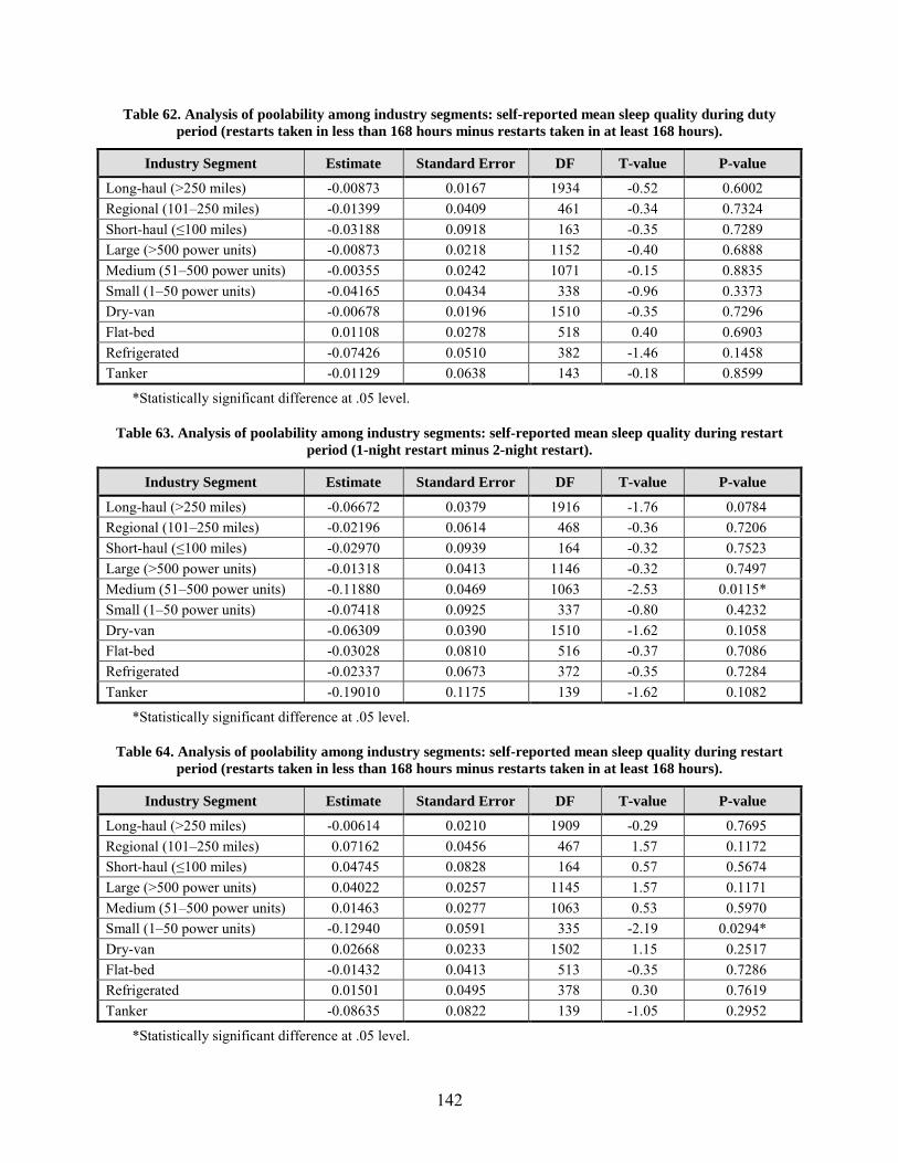
142

Table 62. Analysis of poolability among industry segments: self-reported mean sleep quality during duty period (restarts taken in less than 168 hours minus restarts taken in at least 168 hours).


Long-haul (>250 miles) -0.00873 0.0167 1934 -0.52 0.6002 Regional (101–250 miles) -0.01399 0.0409 461 -0.34 0.7324 Short-haul (≤100 miles) -0.03188 0.0918 163 -0.35 0.7289 Large (>500 power units) -0.00873 0.0218 1152 -0.40 0.6888 Medium (51–500 power units) -0.00355 0.0242 1071 -0.15 0.8835 Small (1–50 power units) -0.04165 0.0434 338 -0.96 0.3373 Dry-van -0.00678 0.0196 1510 -0.35 0.7296 Flat-bed 0.01108 0.0278 518 0.40 0.6903 Refrigerated -0.07426 0.0510 382 -1.46 0.1458 Tanker -0.01129 0.0638 143 -0.18 0.8599


Table 63. Analysis of poolability among industry segments: self-reported mean sleep quality during restart period (1-night restart minus 2-night restart).


Long-haul (>250 miles) -0.06672 0.0379 1916 -1.76 0.0784 Regional (101–250 miles) -0.02196 0.0614 468 -0.36 0.7206 Short-haul (≤100 miles) -0.02970 0.0939 164 -0.32 0.7523 Large (>500 power units) -0.01318 0.0413 1146 -0.32 0.7497 Medium (51–500 power units) -0.11880 0.0469 1063 -2.53 0.0115* Small (1–50 power units) -0.07418 0.0925 337 -0.80 0.4232 Dry-van -0.06309 0.0390 1510 -1.62 0.1058 Flat-bed -0.03028 0.0810 516 -0.37 0.7086 Refrigerated -0.02337 0.0673 372 -0.35 0.7284 Tanker -0.19010 0.1175 139 -1.62 0.1082


Table 64. Analysis of poolability among industry segments: self-reported mean sleep quality during restart period (restarts taken in less than 168 hours minus restarts taken in at least 168 hours).


Long-haul (>250 miles) -0.00614 0.0210 1909 -0.29 0.7695 Regional (101–250 miles) 0.07162 0.0456 467 1.57 0.1172 Short-haul (≤100 miles) 0.04745 0.0828 164 0.57 0.5674 Large (>500 power units) 0.04022 0.0257 1145 1.57 0.1171 Medium (51–500 power units) 0.01463 0.0277 1063 0.53 0.5970 Small (1–50 power units) -0.12940 0.0591 335 -2.19 0.0294* Dry-van 0.02668 0.0233 1502 1.15 0.2517 Flat-bed -0.01432 0.0413 513 -0.35 0.7286 Refrigerated 0.01501 0.0495 378 0.30 0.7619 Tanker -0.08635 0.0822 139 -1.05 0.2952


143

Table 65. Analysis of poolability among industry segments: mean work hours/day in duty period as determined through ELD data (1-night restart minus 2-night restart).


Long-haul (>250 miles) 0.03005 0.1180 2284 0.25 0.7990 Regional (101–250 miles) 0.24870 0.1710 562 1.45 0.1465 Short-haul (≤100 miles) 0.04460 0.3089 245 0.14 0.8853 Large (>500 power units) 0.22640 0.1160 1504 1.95 0.0512 Medium (51–500 power units) 0.00887 0.1637 1187 0.05 0.9568 Small (1–50 power units) -0.12960 0.2952 393 -0.44 0.6609 Dry-van 0.09086 0.1159 1846 0.78 0.4331 Flat-bed 0.01381 0.2328 557 0.06 0.9527 Refrigerated -0.04181 0.2526 515 -0.17 0.8686 Tanker 0.19990 0.3376 148 0.59 0.5546


Table 66. Analysis of poolability among industry segments: mean work hours/day in duty period as determined through ELD data (restarts taken in less than 168 hours minus restarts taken in at least 168

hours).


Long-haul (>250 miles) -0.04537 0.0661 2264 -0.69 0.4928 Regional (101–250 miles) 0.04714 0.1271 555 0.37 0.7109 Short-haul (≤100 miles) 0.69610 0.2622 246 2.65 0.0085* Large (>500 power units) 0.05376 0.0735 1499 0.73 0.4645 Medium (51–500 power units) 0.17620 0.0952 1182 1.85 0.0645 Small (1–50 power units) -0.19820 0.1904 387 -1.04 0.2985 Dry-van 0.10810 0.0701 1833 1.54 0.1235 Flat-bed 0.02499 0.1174 547 0.21 0.8315 Refrigerated 0.12350 0.1817 524 0.68 0.4968 Tanker -0.39260 0.2387 148 -1.64 0.1022


144

Table 67. Analysis of poolability among industry segments: mean driving hours/day in duty period as determined through ELD data (1-night restart minus 2-night restart).


Long-haul (>250 miles) 0.13910 0.1187 2298 1.17 0.2415 Regional (101–250 miles) 0.10630 0.1467 557 0.72 0.4692 Short-haul (≤100 miles) 0.15000 0.2446 245 0.61 0.5403 Large (>500 power units) 0.14980 0.1069 1518 1.40 0.1612 Medium (51–500 power units) 0.24010 0.1643 1167 1.46 0.1443 Small (1–50 power units) 0.00792 0.2815 398 0.03 0.9776 Dry-van 0.09266 0.1157 1862 0.80 0.4231 Flat-bed 0.11730 0.2289 555 0.51 0.6085 Refrigerated 0.17810 0.2065 514 0.86 0.3889 Tanker 0.58110 0.3638 148 1.60 0.1123


Table 68. Analysis of poolability among industry segments: mean driving hours/day in duty period as determined through ELD data (restarts taken in less than 168 hours minus restarts taken in at least 168

hours).


Long-haul (>250 miles) -0.05508 0.0666 2278 -0.83 0.4080 Regional (101–250 miles) 0.03089 0.1089 554 0.28 0.7767 Short-haul (≤100 miles) 0.32620 0.2076 245 1.57 0.1174 Large (>500 power units) 0.01805 0.0677 1511 0.27 0.7898 Medium (51–500 power units) 0.06397 0.0955 1166 0.67 0.5031 Small (1–50 power units) -0.32480 0.1817 393 -1.79 0.0747 Dry-van 0.01525 0.0701 1845 0.22 0.8277 Flat-bed 0.14740 0.1153 547 1.28 0.2017 Refrigerated -0.17940 0.1488 519 -1.21 0.2287 Tanker -0.34890 0.2572 148 -1.36 0.1770


145

Table 69. Analysis of poolability among industry segments: length of restart period (hours) as determined through ELD data (1-night restart – 2-night restart).


Long-haul (>250 miles) -10.9790 3.5487 2390 -3.09 0.0020* Regional (101–250 miles) -18.3282 3.0367 571 -6.04 <.0001* Short-haul (≤100 miles) -23.9920 4.2308 249 -5.67 <.0001* Large (>500 power units) -15.6274 3.4143 1576 -4.58 <.0001* Medium (51–500 power units) -12.6250 3.4745 1196 -3.63 0.0003* Small (1–50 power units) -6.8325 8.9642 404 -0.76 0.4464 Dry-van -13.7980 2.9434 1891 -4.69 <.0001* Flat-bed -14.0084 6.5236 555 -2.15 0.0322* Refrigerated -13.6418 7.1734 536 -1.90 0.0577 Tanker -4.2213 8.9840 150 -0.47 0.6391


Table 70. Analysis of poolability among industry segments: length of restart period (hours) as determined through ELD data (restarts taken in less than 168 hours minus restarts taken in at least 168 hours).


Long-haul (>250 miles) 0.5165 2.0064 2368 0.26 0.7969 Regional (101–250 miles) 0.6642 2.2815 564 0.29 0.7711 Short-haul (≤100 miles) 9.5274 3.5863 247 2.66 0.0084* Large (>500 power units) 0.5930 2.1856 1584 0.27 0.7862 Medium (51–500 power units) 0.5344 2.0342 1211 0.26 0.7928 Small (1–50 power units) 3.6451 5.8115 395 0.63 0.5309 Dry-van 0.2480 1.8101 1920 0.14 0.8910 Flat-bed 7.7887 3.3364 555 2.33 0.0199* Refrigerated -2.7985 5.0958 548 -0.55 0.5831 Tanker 3.2391 6.3231 150 0.51 0.6092


Table 71. Analysis of poolability among industry segments: length of duty period (hours) as determined through ELD data (1-night restart minus 2-night restart).


Long-haul (>250 miles) -8.0724 5.3910 2298 -1.50 0.1344 Regional (101–250 miles) -0.6984 4.5847 572 -0.15 0.8790 Short-haul (≤100 miles) -3.9710 5.8805 248 -0.68 0.5001 Large (>500 power units) -8.0483 5.4292 1526 -1.48 0.1384 Medium (51–500 power units) -0.4042 5.4203 1194 -0.07 0.9406 Small (1–50 power units) -4.1426 12.2983 397 -0.34 0.7364 Dry-van -6.2399 4.6761 1861 -1.33 0.1822 Flat-bed 4.1499 10.2754 560 0.40 0.6865 Refrigerated -6.0577 9.7566 515 -0.62 0.5350 Tanker 11.3885 14.9937 149 0.76 0.4487


146

Table 72. Analysis of poolability among industry segments: length of duty period (hours) as determined through ELD data (restarts taken in less than 168 hours minus restarts taken in at least 168 hours).


Long-haul (>250 miles) 0.2952 3.0246 2268 0.10 0.9223 Regional (101–250 miles) 3.0173 3.4383 562 0.88 0.3806 Short-haul (≤100 miles) -9.0752 4.9815 247 -1.82 0.0697 Large (>500 power units) -0.4525 3.4424 1514 -0.13 0.8954 Medium (51–500 power units) -0.0983 3.1549 1185 -0.03 0.9751 Small (1–50 power units) -3.8138 7.9610 388 -0.48 0.6322 Dry-van -3.6059 2.8338 1838 -1.27 0.2034 Flat-bed 7.0444 5.1931 549 1.36 0.1755 Refrigerated 0.2870 7.0043 528 0.04 0.9673 Tanker 3.5505 10.5997 149 0.33 0.7381


Table 73. Analysis of poolability among industry segments: adjudicated sleep per 24 hours of duty period (1-night restart minus 2-night restart).


Long-haul (>250 miles) -0.0457 0.0800 1726 -0.57 0.5679 Regional (101–250 miles) -0.1029 0.0998 450 -1.03 0.3030 Short-haul (≤100 miles) -0.2001 0.1981 172 -1.01 0.3140 Large (>500 power units) -0.1105 0.0803 1077 -1.38 0.1694 Medium (51–500 power units) -0.1200 0.1051 954 -1.14 0.2538 Small (1–50 power units) -0.0602 0.1753 298 -0.34 0.7317 Dry-van -0.0374 0.0775 1452 -0.48 0.6290 Flat-bed -0.0348 0.1486 437 -0.23 0.8149 Refrigerated -0.3965 0.1825 306 -2.17 0.0306* Tanker -0.0519 0.1883 124 -0.28 0.7832


Table 74. Analysis of poolability among industry segments: adjudicated sleep per 24 hours of duty period (restarts taken in less than 168 hours minus restarts taken in at least 168 hours).


Long-haul (>250 miles) 0.0477 0.0445 1712 1.07 0.2839 Regional (101–250 miles) -0.0336 0.0775 446 -0.43 0.6649 Short-haul (≤100 miles) -0.2066 0.1695 170 -1.22 0.2245 Large (>500 power units) -0.0022 0.0518 1075 -0.04 0.8954 Medium (51–500 power units) -0.0341 0.0594 953 -0.57 0.5662 Small (1–50 power units) 0.0018 0.1177 297 0.02 0.9876 Dry-van -0.0818 0.0471 1443 -1.74 0.0824 Flat-bed 0.2176 0.0773 434 2.82 0.0051* Refrigerated -0.1287 0.1264 314 -1.02 0.3093 Tanker 0.0959 0.1357 124 0.71 0.4812


147

Table 75. Analysis of poolability among industry segments: adjudicated sleep per 24 hours of restart period (1-night restart minus 2-night restart).


Long-haul (>250 miles) -0.2919 0.1606 1341 -1.82 0.0694 Regional (101–250 miles) 0.6862 0.1966 318 3.49 0.0006* Short-haul (≤100 miles) 0.3247 0.2672 158 1.22 0.2261 Large (>500 power units) 0.5133 0.1633 791 3.14 0.0017* Medium (51–500 power units) -0.4757 0.1966 758 -2.42 0.0158* Small (1–50 power units) -0.8713 0.3015 260 -2.89 0.0042* Dry-van 0.2050 0.1496 1086 1.37 0.1708 Flat-bed -0.4696 0.3572 360 -1.31 0.1894 Refrigerated 0.0117 0.2665 253 0.04 0.9649 Tanker -0.1642 0.3455 102 -0.48 0.6357


Table 76. Analysis of poolability among industry segments: adjudicated sleep per 24 hours of restart period (restarts taken in less than 168 hours minus restarts taken in at least 168 hours).


Long-haul (>250 miles) -0.1376 0.0899 1334 -1.53 0.1263 Regional (101–250 miles) -0.1687 0.1575 311 -1.07 0.2849 Short-haul (≤100 miles) -0.4536 0.2430 156 -1.87 0.0638 Large (>500 power units) -0.1370 0.1068 791 -1.28 0.1999 Medium (51–500 power units) -0.0734 0.1089 759 -0.67 0.5008 Small (1–50 power units) -0.0862 0.2202 256 -0.39 0.6956 Dry-van -0.2217 0.0927 1075 -2.39 0.0169* Flat-bed -0.2979 0.1698 356 -1.75 0.0802 Refrigerated 0.3793 0.2180 260 1.74 0.0831 Tanker -0.0838 0.2484 102 -0.34 0.7366


Table 77. Analysis of poolability among industry segments: PVT-B mean reciprocal response time in the duty period (1-night restart minus 2-night restart).


Long-haul (>250 miles) 0.0119 0.0192 2041 0.62 0.5363 Regional (101–250 miles) -0.0585 0.0345 533 -1.69 0.0907 Short-haul (≤100 miles) 0.0238 0.0446 210 0.53 0.5936 Large (>500 power units) -0.0296 0.0237 1332 -1.25 0.2118 Medium (51–500 power units) 0.0247 0.0255 1128 0.97 0.3339 Small (1–50 power units) 0.0281 0.0301 350 0.93 0.3516 Dry-van -0.0175 0.0221 1712 -0.79 0.4288 Flat-bed 0.0195 0.0358 514 0.55 0.5859 Refrigerated 0.0281 0.0321 389 0.87 0.3826 Tanker 0.0117 0.0373 141 0.31 0.7539


148

Table 78. Analysis of poolability among industry segments: PVT-B mean reciprocal response time in the duty period (restarts taken in less than 168 hours minus restarts taken in at least 168 hours).


Long-haul (>250 miles) 0.0148 0.0106 1996 1.40 0.1627 Regional (101–250 miles) 0.0084 0.0258 526 0.33 0.7448 Short-haul (≤100 miles) 0.0718 0.0376 212 1.91 0.0573 Large (>500 power units) 0.0187 0.0148 1284 1.27 0.2061 Medium (51–500 power units) 0.0326 0.0146 1103 2.23 0.0261* Small (1–50 power units) -0.0258 0.0196 345 -1.32 0.1870 Dry-van 0.0243 0.0132 1669 1.85 0.0650 Flat-bed 0.0147 0.0181 523 0.81 0.4176 Refrigerated 0.0231 0.0232 377 1.00 0.3194 Tanker -0.0486 0.0260 136 -1.87 0.0636


Table 79. Analysis of poolability among industry segments: PVT-B mean reciprocal response time in the restart period (1-night restart minus 2-night restart).


Long-haul (>250 miles) 0.0117 0.0231 2331 0.50 0.6143 Regional (101–250 miles) -0.0078 0.0404 570 -0.19 0.8473 Short-haul (≤100 miles) 0.0297 0.0455 225 0.65 0.5150 Large (>500 power units) 0.0164 0.0272 1492 0.60 0.5453 Medium (51–500 power units) -0.0081 0.0299 1260 -0.27 0.7855 Small (1–50 power units) 0.0356 0.0437 380 0.81 0.4157 Dry-van -0.0059 0.0251 1939 -0.24 0.8126 Flat-bed 0.0945 0.0477 573 1.98 0.0480* Refrigerated 0.0330 0.0360 452 0.92 0.3601 Tanker -0.0178 0.0614 142 -0.29 0.7721


Table 80. Analysis of poolability among industry segments: PVT-B mean reciprocal response time in the restart period (restarts taken in less than 168 hours minus restarts taken in at least 168 hours).


Long-haul (>250 miles) 0.0296 0.0125 2080 2.37 0.0180* Regional (101–250 miles) 0.0115 0.0295 497 0.39 0.6962 Short-haul (≤100 miles) 0.0108 0.0360 187 0.30 0.7654 Large (>500 power units) 0.0297 0.0167 1326 1.78 0.0755 Medium (51–500 power units) 0.0322 0.0166 1093 1.94 0.0528 Small (1–50 power units) -0.0051 0.0277 336 -0.18 0.8554 Dry-van 0.0309 0.0147 1702 2.10 0.0354* Flat-bed 0.0366 0.0237 527 1.55 0.1220 Refrigerated 0.0125 0.0249 383 0.50 0.6151 Tanker -0.0240 0.0418 125 -0.57 0.5669


149

REFERENCES 1. Pub. L. 113-235, 128 Stat. 2130, 2712, December 16, 2014.

2. Verbeke, G & Molenberghs, G. (2000). Linear Mixed Models for Longitudinal Data. New York: Springer.

3. Diggle, P.J., Liang, K.Y., & Zeger, S.L. (1996). Analysis of Longitudinal Data. New York: Oxford University Press.

4. Stroup, W.W. (2013). Generalized Linear Mixed Models: Modern Concepts, Methods and Applications. Boca Raton: CRC Press.

5. Dinges, D.F., Maislin, G. Brewster, R.M., Krueger, G.P., & Carroll, R.J. (2005). Pilot test of fatigue management technologies. Transportation Research Record: Journal of the Transportation Research Board . No. 1922, Transportation Research Board of the National Academies, Washington, DC, 175–182.

6. Van Dongen, H., & Mollicone, D.J. (2014). Field Study on the Efficacy of the New Restart Provision for Hours of Service (No. RRR-13-058).

7. Hanowski, R.J., Hickman, J.S., Fumero, M.C., Olson, R.L., & Dingus, T.A. (2007). The sleep of commercial motor vehicle drivers under the 2003 hours-of-service regulations. Accident Analysis and Prevention 39, 1140–1145.

8. Ford, E.S., Cunningham, T.J., Croft, J.B., et al. (2015). Trends in self-reported sleep duration among US adults from 1985 to 2012. Sleep, 38, 829–832.

9. Watson, N.F., Badr, M.S., Belenky, G., Bliwise, D.L., Buxton, O.M., Buysse, D., Dinges, D.F., Gangwisch, J., Grandner, M.A., Kushida, C., Malhotra, R.K., Martin, J.L., Patel, S.R., Quan, S.F., Tasali, E. (2015a). Recommended amount of sleep for a healthy adult: A joint consensus statement of the American Academy of Sleep Medicine and Sleep Research Society. Sleep, 38(6), 843–844.

10. Watson, N.F., Badr, M.S., Belenky, G., Bliwise, D.L., Buxton, O.M., Buysse, D., Dinges, D.F., Gangwisch, J., Grandner, M.A., Kushida, C., Malhotra, R.K., Martin, J.L., Patel, S.R., Quan, S.F., Tasali, E. (2015b). Joint consensus statement of the American Academy of Sleep Medicine and Sleep Research Society on the recommended amount of sleep for a healthy adult: Methodology and discussion. Sleep 38(8), 1161–1183.

11. Dinges, et al. 2005.

12. Van Dongen & Mollicone. 2014.

13. Dinges, et al., 2005.

14. Abe, T., Mollicone, D., Basner, M., & Dinges, D.F. (2014). Sleepiness and safety: Where biology needs technology. Sleep and Biological Rhythms, 12, 74–84.

150

15. Balkin, T., Horrey, W.J., Graeber, R.C., Czeisler, C.A., & Dinges, D.F. (2011). The

challenges and opportunities of technological approaches to fatigue management. Accident Analysis and Prevention 43, 565, 572.

16. Dinges, D.F., & Abe, T. (2013). Transportation Safety and Operator Sleepiness: Where Biology Needs Technology. Proceedings of the International Association of Traffic and Safety Sciences (IATSS), 88–120.

17. Hanowski, R.J., Hickman, J.H., Olson, R.L., & Bocanegra, J. (2009). Evaluating the 2003 revised hours-of-service regulations for truck drivers: The impact of time-on-task on critical incident risk. Accident Analysis and Prevention, 41, 268–275.

18. Dinges, D.F. (1995). An overview of sleepiness and accidents. J Sleep Research, 4 (Sup 2), 4–14.

19. Brown, I.D. (1994) Driver fatigue. Human Factors 36 (2), 298–314.

20. Hanowski, Hickman, Olson, & Bocanegra, 2009.

21. Basner, M., Mollicone, D., & Dinges, D.F. (2011). Validity and sensitivity of a Brief Psychomotor Vigilance Test (PVT-B) to total and partial sleep deprivation. Acta Astronautica, 69, 949–59.

22. Philip, P. et al. (2008). Maintenance of wakefulness test, obstructive sleep apnea syndrome, and driving risk. Annals of Neurology, 64 (4), 410–416.

23. Van Dongen & Mollicone, 2014.

24. Darwent, D., Roach, G., & Dawson, D. (2012). How well do truck drivers sleep in cabin sleeper berths? Applied Ergonomics, 43, 442–446.


26. Cappuccio, F.P., D’Elia, L., Strazzullo, P., & Miller, M.A. (2010). Sleep duration and all-cause mortality: A systematic review and meta-analysis of prospective studies. Sleep, 33 (5), 585–592.

27. Edwards, R.R., et al. (2008). Duration of sleep contributes to next-day pain report in the general population. Pain, 137 (1), 202–207.

28. Hoevenaar- Blom, M.P., Spijkerman, A.M., Kromhout, D., van den Berg, J.F., Vershuren W.M. (2011). Sleep duration and sleep quality in relation to 12-year cardiovascular disease incidence: The MORGEN Study. Sleep, 34 (11), 1487–1492.

29. Grandner, M.A., Chakravorty, S., Perlis, M.L., Oliver, L., Gurubhagavatula, I. (2014). Habitual sleep duration associated with self-reported and objectively determined cardiometabolic risk factors. Sleep Medicine, 15, 42–50.

30. Knutsson, A. (2003). Health disorders of shift workers. Occupat.Medicine-Oxford, 53 (2), 103–108.

151

31. Wang, Q., Xi, B., Liu, M., Zhang, M., Fu, M. (2012). Short sleep duration is associated with

hypertension risk among adults: A systematic review and meta-analysis. Hypertension Research, 35, 1012–1018.

32. Akerstedt, T., Kecklund, G, Gillberg M. (2007). Sleep and sleepiness in relation to stress and displaced work hours. Physiology & Behavior, 92 (1−2), 250–255.

33. Jeon, H.J., Kim, J.H., Kim, B.N., Park, S.J., Fava, M., Mischoulon, D., Choi, H., Roh, S., Lee, D. (2014). Sleep quality, posttraumatic stress, depression, and human errors in train drivers: A population-based nationwide study in South Korea. Sleep, 37(12), 1969–75.


35. Dinges, D.F., & Powell, J.W. (1985). Microcomputer analyses of performance on a portable, simple visual RT task during sustained operations. Behavior Research Methods, Instruments, & Computers, 17(6), 652−655.

36. Lim, J., & Dinges, D.F. (2008). Sleep deprivation and vigilant attention. Annals of the New York Academy of Sciences, 1129, 305–322.

37. Basner, M., & Dinges, D.F. (2011). Maximizing sensitivity of the Psychomotor Vigilance Test (PVT) to sleep loss. Sleep, 34(5), 581–591.

38. Dorrian, J., Rogers, N.L., & Dinges, D.F. (2005). Psychomotor vigilance performance: Neurocognitive assay sensitive to sleep loss. In C.A. Kushida (Ed.), Sleep deprivation: Clinical issues, pharmacology, and sleep loss effects (pp. 39-70). Boca Raton, FL: CRC Press.

39. Balkin, T.J., et al. (2004). Comparative utility of instruments for monitoring sleepiness-related performance decrements in the operational environment. J Sleep Res, 13, 219–227.

40. Basner, Mollicone, & Dinges, 2011.

41. Basner, M., Dinges, D.F., et al. (2014). Psychological and behavioral changes during confinement in a 520-day simulated interplanetary mission to Mars. PLoS ONE, 9 (3): e93298.


43. Shankar, V., Jovanis, P.P., & Aguero-Valverde, J. (2008). Analysis of naturalistic driving data: prospective view on methodological paradigms. Transportation Research Record, 2061, 1–8.

44. Cohen, J. (1988). Statistical power analysis for the behavioral sciences (2nd ed.). New York: Academic Press.

45. Wierwille, W.W. & Ellsworth, L.A. (1994). Evaluation of driver drowsiness by trained observers. Accident Analysis and Prevention, 26(5), 571–581.

46. Shankar, Jovanis, & Aguero-Valverde, 2008.

152

47. Federal Motor Carrier Safety Administration (2015). Federal Motor Carrier Safety

Administration Commercial Motor Vehicle Driver Restart Study Plan. Retrieved from: https://www.fmcsa.dot.gov/sites/fmcsa.dot.gov/files/docs/UPDATED%20-%20CMV%20Driver%20Restart%20Study%20Plan.pdf.

48. Verbeke & Molenberghs, 2000.

49. Diggle, Liang, & Zeger, 1996.

50. Stroup, 2013.

51. Dinges, D.F. (2015). Neurobehavioral dynamics of human sleep restriction and recovery. Invited Lecture in Symposium entitled: How do repeated patterns of insufficient and recovery sleep affect physiological, subjective and nuerobehavioral domains? Presented at SLEEP 2015 on June 7, 2015.

52. Zhou, Z., & Lam, P. (2007). Discussion of: Statistical and regulatory issues with the application of propensity score analysis to nonrandomized medical device clinical studies. J of Biopharmaceutical Statistics, 17, 25–27.

53. Rubin, D. (2008).

54. Yue, L.Q. (2007). Statistical and regulatory issue with the application of propensity score analysis to nonrandomized medical device clinical studies, Journal of Biopharmaceutical Statistics, 17, 1–13.

55. Jovanis, P.P., Wu, K-F, & Chen, C. (2011). Hours of service and driver fatigue: Driver characteristics research. Report No. FMCSA-RR-11-018. U.S. Department of Transportation, Washington, D.C.

56. American Trucking Associations. (2014). Driver Compensation Study.

57. Sieber, W.K., Robinson, C.F., Birdsey, J., Chen, G.X., Hitchcock, E.M., Lincoln, J.E., Nakata, A., & Sweeney, M.H. (2014). American Journal of Industrial Medicine, 57, 615–626.

58. Thiese, M.S., Moffit, G., Hanowski, R.J., Kales, S.N., Porter, R.J., & Hegmann, K.T. (2015). Commercial driver medical examinations: Prevelance of Obesity, comorbidities, and certification outcomes. Journal of Occupational and Environmental Medicine, 57(6), 659–665.

59. Lim & Dinges, 2008.

60. Watson et al. 2015a.

61. Watson et al. 2015b.

62. Ford, 2015.

63. Dinges, D.F., Maislin, G. Brewster, R.M., Krueger, G.P., & Carroll, R.J. (2005). Pilot test of fatigue management technologies. Transportation Research Record: Journal of the Transportation Research Board No. 1922, Transportation Research Board of the National Academies, Washington, DC, 175–182.

https://www.fmcsa.dot.gov/sites/fmcsa.dot.gov/files/docs/UPDATED%20-%20CMV%20Driver%20Restart%20Study%20Plan.pdf

https://www.fmcsa.dot.gov/sites/fmcsa.dot.gov/files/docs/UPDATED%20-%20CMV%20Driver%20Restart%20Study%20Plan.pdf

153

64. Van Dongen, H., & Mollicone, D.J. (2014). Field Study on the Efficacy of the New Restart

Provision for Hours of Service (No. RRR-13-058).

65. Hanowski, R.J., Hickman, J.S., Fumero, M.C., Olson, R.L., & Dingus, T.A. (2007). The sleep of commercial motor vehicle drivers under the 2003 hours-of-service regulations. Accident Analysis and Prevention 39, 1140–1145.


67. Wu, K.F., & Jovanis, P. (2011). Effect of driving breaks and 34-hour recovery period on motor carrier crash odds. In Proceedings of 6th International Driving Symposium on Human Factors in Driver Assessment, Training, and Vehicle Design.

68. Barr, L.C., Yang, C.Y.D., Hanowski, R.J., & Olson, R. (2011). An assessment of driver drowsiness, distraction, and performance in a naturalistic setting. Report No. FMCSA-RRR-11-010. U.S. Department of Transportation, Washington, D.C.

69. Pack, A.I., Pack, A.M., Rodgman, E., Cucchiara, A., Dinges, D.F., & Schwab, C.W. (1995). Characteristics of crashes attributed to the driver having fallen asleep. Accident Analysis & Prevention 27(6), 769–775.

70. Lim & Dinges, 2008.

71. Mollicone, D.J., Van Dongen, H., Rogers, N.L., Banks, S., Dinges, D.F. (2010). Time of day modulates the effects of chronic sleep restriction on neurobehavioral performance. Aviation, Space & Environmental Medicine, 81, 735–744, August.

72. Cohen, D.A., Wang, W., Wyatt, J.K., Kronauer, R.E., Dijk, D-J, Czeisler, CA, Klerman, E.B. (2010). Uncovering Residual Effects of Chronic Sleep Loss on Human Performance. Science Translational Medicine, 2(14), 1–9.

73. Jewett, M.E., Wyatt, J.K., Ritz-De Cecco, A., Khalsa, S.B., Dijk, D.J., Czeisler, C.A. (1999). Time course of sleep inertia dissipation in human performance and alertness. Journal of Sleep Research 8, 1–8.

74. Blanco, M., Hanowski, R.J., Olson, R.L., Morgan, J.F., Soccolich, S.A., Wu, S-C, & Guo, F. (2011). The impact of driving, non-driving work, and rest breaks on driving performance in commercial motor vehicle operations. Virginia Tech Transportation Institute, Blacksburg, VA.

75. Short, J. (2013). Assessing the impacts of the 34-hour restart provisions. American Transportation Research Institute (ATRI), Arlington, VA.

76. Soccolich, S.A., Blanco, M., Hanowski, R.J., Olson, R.L., Morgan, J.F., Guo, F., & Wu, S.C. (2013). An analysis of driving and working hour on commercial motor vehicle driver safety using naturalistic data collection. Accident Analysis and Prevention 58, 249–258.

77. Federal Motor Carrier Safety Administration (FMCSA). (2011). 2010–2011 Hours of Service Rule Regulatory Impact Analysis (RIA). RIN 2126-AB26, FMCSA Analysis Division, Washington, D.C.

154

78. Federal Motor Carrier Safety Administration (FMCSA), 2011.



81. Hanowski, R.J., et al. 2007.

82. Belenky, G., Wesensten, N.J., Thorne, D.R., Thomas, M.L., Sing, H.C., Redmond, D.P., Russo, M.B., & Balkin, T.J. (2003). Patterns of performance degradation and restoration during sleep restriction and subsequent recovery: A sleep dose–response study. Sleep Res. 12, 1-12.

83. Van Dongen, H.P.A., Maislin, G., Mullington, J.M., & Dinges, D.F. (2003). The cumulative cost of additional wakefulness: Dose-response effects on neurobehavioral functions and sleep physiology from chronic sleep restriction and total sleep deprivation. Sleep 26 (2), 117-126.

84. Dinges, D.F. (2015). Neurobehavioral dynamics human sleep restriction and recovery. Invited Lecture in Symposium entitled: How do repeated patterns of insufficient and recovery sleep affect physiological, subjective and neurobehavioral domains? Presented at SLEEP 2015, 10:30–12:30, 7 June 2015.





89. Hanowski, et al., 2007.




93. Hanowski, et al., 2007.



96. Lauderdale, D.S., Knutson. K.L., Yan, L.L., & Rathouza, P.J. (2008). Self-reported and measured sleep duration: How similar are they? Epidemiology 19, 838–845.

97. Basner, M., Dinges, D.F., Mollicone, D.J., Ecker, A.J., Jones, C.W., Hyder, E., Di Antonio, A., Savelev, I., Kan, K., Goel, N., Morukov, B.V., & Sutton, J.P. (2013). Mars 520-d mission simulation reveals protracted crew hypokinesis and alterations of sleep duration and timing. Proceedings of the National Academies of Sciences of the USA 110 (7): 2635–2640, Supporting Information, 5–6.

98. Thiffault, P. (2011). Addressing human factors in the motor carrier industry in Canada. Canadian Council of Motor Transport Administrators (CCMTA).

155

99. Blanco, M., Hickman, J., Olson, R., Bocanegra, J., Hanowski, R. J., Nakata, A., et al. (in

press). Investigating critical incidents, driver restart period, sleep quantity, and crash countermeasures in commercial vehicle operations using naturalistic data collection. Washington, DC: Federal Motor Carrier Safety Administration, USDOT.

100. Anderson, C., & Horne, J.A. (2006). Sleepiness enhances distraction during a monotonous task. Sleep 29 (4), 573–576.

101. Thiffault, 2011.

102. Baulk, S.D., & Fletcher, A. (2012). At home and away: Measuring the sleep of Australian truck drivers. Accident Analysis and Prevention 45S, 36–40.

103. Knutsson, 2003.

104. Abe, Mollicone, Basner, & Dinges, 2014.

105. Dinges, et al., 2005.


107. Balkin, et al., 2011.

108. Dinges & Abe, 2013.

109. Dinges, et al., 2005.


111. Barr, Yang, Hanowski & Olson, 2011.

112. Dinges, et al., 2005.

113. Mallis, M.M., Banks, S., & Dinges, D.F. (2010). Aircrew fatigue and circadian rhythmicity. In.: Salas, E. & Maurino D. (Eds.), Chapter 13: Human Factors in Aviation (2nd ed.). Elsevier: Academic Press, 401–436.

114. Raslear, T.G., Gertler, J., & DiFiore, A. (2013). Work schedules, sleep, fatigue, and accidents in the US railroad industry. Fatigue: Biomedicine, Health & Behavior 1, 99–115.

115. Ogden, C.L., Carroll, M.D., Kit, B.K., & Flegal, K.M. (2014). Prevalence of childhood and adult obesity in the United States, 2011–2012. Journal of the American Medical Association, 311(8), 806-814.

116. Bonauto, D.K., Lu, D.Y., & Fan, Z.J. (2014). Obesity Prevalence by Occupation in Washington State, Behavioral Risk Factor Surveillance System. Preventing Chronic Disease, 11.

117. Thiese, M.S., Moffitt, G., Hanowski, R.J., Kales, S.N., Porter, R.J., & Hegmann, K.T. (2015). Commercial Driver Medical Examinations: Prevalence of Obesity, Comorbidities, and Certification Outcomes. Journal of Occupational and Environmental Medicine.

118. Thiese, et al., 2015.

156

119. Pack, A.I., Maislin, G., Staley, B., Pack, F.M., Rogers, W., George, C.F.P., & Dinges, D.F.

(2006). Impaired performance in commercial drivers: Role of sleep apnea and sleep duration. American Journal of Respiratory and Critical Care Medicine, 174, 446–454.

120. Catarino, R., Spratley, J., Catarino, I., Lunet, N., & Pais-Clemente, M. (2014). Sleepiness and sleep-disordered breathing in truck drivers. Risk analysis of road accidents. Sleep Breath 18, 59–68.

121. Wiegand, D.M., Hanowski, R.J., & McDonald, S.E. (2009). Commercial drivers’ health: A naturalistic study of body mass index, fatigue, and involvement in safety-critical events. Traffic Injury Prevention, 10, 573-579.

122. Anderson, J.E., et al. (2012). Obesity is associated with the future risk of heavy truck crashes among newly recruited commercial drivers. Accident Analysis & Prevention, 49, 378-384.

123. Bonauto, Lu & Fan, 2014.

124. U.S. Department of Transportation, Office of Management and Budget. (December 16, 2004). Final Information Quality Bulletin for Peer Review.

125. National Academy of Sciences. (May, 2003). Policy and Procedures on Committee Composition and Balance and Conflicts of Interest for Committees Used in the Development of Reports.

126. Verbeke & Molenberghs, 2000.

127. Diggle, Liang, & Zeger, 1996.

128. Stroup, 2013.

commercial motor vehicle driver restart study: final report driver restart...naturalistic study of...

Documents