combining remote sensing and gis climate modelling to

Hydrol. Earth Syst. Sci., 15, 1563–1575, 2011www.hydrol-earth-syst-sci.net/15/1563/2011/doi:10.5194/hess-15-1563-2011© Author(s) 2011. CC Attribution 3.0 License.

Hydrology andEarth System

Sciences

Combining remote sensing and GIS climate modelling to estimatedaily forest evapotranspiration in a Mediterranean mountain area

J. Cristobal1,4, R. Poyatos2, M. Ninyerola1, P. Llorens3, and X. Pons4

1Department of Animal Biology, Plant Biology and Ecology, C-Building, Universitat Autonoma de Barcelona,Cerdanyola del Valles, 08193, Spain2Center for Ecological Research and Forestry Applications (CREAF), Universitat Autonoma de Barcelona,Cerdanyola del Valles, 08193, Spain3Institute of Environmental Assessment and Water Research (IDÆA), CSIC, Jordi Girona, 18, Barcelona, 08034, Spain4Department of Geography, B-Building, Universitat Autonoma de Barcelona, Cerdanyola del Valles, 08193, Spain

Received: 13 December 2010 – Published in Hydrol. Earth Syst. Sci. Discuss.: 25 January 2011Revised: 26 April 2011 – Accepted: 7 May 2011 – Published: 25 May 2011

Abstract. Evapotranspiration monitoring allows us to assessthe environmental stress on forest and agricultural ecosys-tems. Nowadays, Remote Sensing and Geographical Infor-mation Systems (GIS) are the main techniques used for cal-culating evapotranspiration at catchment and regional scales.In this study we present a methodology, based on the energybalance equation (B-method), that combines remote sensingimagery with GIS-based climate modelling to estimate dailyevapotranspiration (ETd) for several dates between 2003 and2005. The three main variables needed to compute ETd wereobtained as follows: (i) Land surface temperature by meansof the Landsat-5 TM and Landsat-7 ETM+ thermal band,(ii) air temperature by means of multiple regression analy-sis and spatial interpolation from meteorological ground sta-tions data at satellite pass, and (iii) net radiation by means ofthe radiative balance. We calculated ETd using remote sens-ing data at different spatial and temporal scales (Landsat-7ETM+, Landsat-5 TM and TERRA/AQUA MODIS, with aspatial resolution of 60, 120 and 1000 m, respectively) andcombining three different approaches to calculate theB pa-rameter, which represents an average bulk conductance forthe daily-integrated sensible heat flux. We then comparedthese estimates with sap flow measurements from a Scotspine (Pinus sylvestrisL.) stand in a Mediterranean moun-tain area. This procedure allowed us to better understandthe limitations of ETd modelling and how it needs to be im-proved, especially in heterogeneous forest areas. The method

Correspondence to:J. Cristobal([email protected])

using Landsat data resulted in a good agreement,R2 test of0.89, with a mean RMSE value of about 0.6 mm day−1 andan estimation error of±30 %. The poor agreement obtainedusing TERRA/AQUA MODIS, with a mean RMSE value of1.8 and 2.4 mm day−1 and an estimation error of about±57and 50 %, respectively. This reveals that ETd retrieval fromcoarse resolution remote sensing data is troublesome in theseheterogeneous areas, and therefore further research is neces-sary on this issue. Finally, implementing regional GIS-basedclimate models as inputs in ETd retrieval have has providedgood results, making possible to compute ETd at regionalscales.

1 Introduction

Evaporation and transpiration are the two main processes in-volved in water transfer from vegetated areas to the atmo-sphere. Evapotranspiration (ET) from the Earth’s vegeta-tion constitutes 88 % of the total terrestrial evapotranspira-tion, and returns more than 50 % of terrestrial precipitationto the atmosphere (Oki and Kanae, 2006); therefore it playsa key role in both the hydrological cycle and the energy bal-ance of the land surface. Climate warming may acceleratethe hydrological cycle as a result of enhanced evaporativedemand in some regions where water is not limiting (Junget al., 2010). However, the combination of warmer tempera-tures with constant or reduced precipitation in other regionsmay lead to a large decrease in water availability for naturaland agricultural systems as well as for human needs (Jackson

Published by Copernicus Publications on behalf of the European Geosciences Union.

http://creativecommons.org/licenses/by/3.0/

1564 J. Cristobal et al.: Combining remote sensing and GIS climate modelling to estimate daily forest ET

et al., 2001), especially in arid or semiarid areas (Jung et al.,2010) such as the Mediterranean basin (Bates et al., 2008).

Evapotranspiration has been measured extensively at localscales using micrometeorological (such as eddy-covarianceor the Bowen ratio) or sap flow techniques. Since the lastdecade, there have been several global initiatives to moni-tor evapotranspiration in different vegetation types, such asFLUXNET (ORNL DAAC, 2010). Therefore, magnitudesand controls (climate, water availability, physiological regu-lation, etc.) on evapotranspiration are widely known for dif-ferent types of vegetation, albeit at small spatial scales. Howcan we improve, then, our knowledge of evapotranspiration?In terms of spatial variability (and its driving factors) the nextchallenge is larger scales.

ET can be modelled at global scales using GIS climate-based methodologies such as GIS-based Environmental Pol-icy Integrated Climate – GEPIC – (Liu et al., 2007, 2009),Lund-Potsdam-Jena managed Land – LPJmL – (Rost et al.,2008) or Global Crop Water Model – GCWM – (Siebert andDoll, 2010). However, radiometric measurements providedby remote sensing added to GIS-based climate modellinghave proved to be essential for modelling ET because theyare the only techniques that allow us to compute it feasiblyat both regional (Cristobal et al., 2005; Kustas and Norman,1996) and global scales (Mu et al., 2007). Moreover, theuse of remote sensing techniques supplements the frequentlack of ground-measured variables and parameters that arerequired for applying the local models at a regional scale(Sanchez et al., 2008a).

Currently, there are a wide variety of remote sensingmodels for calculating ET at global or regional scales,such as METRIC (Allen et al., 2007), SEBAL (Basti-aanssen et al., 1998), TSEB (Kustas and Norman, 2000),ALEXI/disALEXI (Anderson et al., 2004), S-SEBI (Roerinket al., 2000), STSEB (Sanchez et al., 2008b) and the B-Method (Jackson et al., 1977; Seguin and Itier, 1983); othermethodologies can be found in Schmugge et al. (2002) orSanchez et al. (2008a). All these theoretical methods usedto estimate ET at a regional scale with remote sensing tech-niques are derived from the energy balance equation based onthe principle of energy conservation in a system formed bysoil and vegetation. Most of them try to minimize the inputsfrom ancillary data (often data from ground meteorologicalstations) in order to make the algorithms more operationalat global scales. However, there is currently no agreementon which method is the most appropriate because this oftendepends on the application purposes.

Most of these methods have been validated in homoge-neous covers (crops or natural vegetation) and flat areas,where a single meteorological station record is used to de-scribe the climate conditions of a large area. In these ar-eas, the use of moderate or coarse spatial resolution remotesensing data is enough to obtain accurate daily ET (ETd)results. However, in more complex and heterogeneous ar-eas, due to the landscape, orographic or climatic variability,

a single meteorological record or remote sensing data withcoarse spatial resolution may not be accurate enough to cal-culate the ETd. Operative GIS climate-based techniques canbe used at regional scales in both simple and complex areas(Ninyerola et al., 2007; Pons and Ninyerola, 2008) to achievehigher accuracy and provide the input variables for agricul-ture and natural vegetation evapotranspiration modelling.

The objective of this paper is to evaluate a simple methodfor computing daily ET using stand-scale sap flow mea-surements made in Scots Pine (Pinus sylvestrisL.) in aheterogeneous Mediterranean mountain area during a threeyear period. GIS climate-based regional modelling wasused instead of a single meteorological measurement toobtain the meteorological inputs (air temperature and so-lar radiation) in order to evaluate the performance of thistechnique. Low (TERRA/AQUA MODIS) and moderate(Landsat-TM/ETM+) spatial resolution remote sensing im-ages were used as the remote sensing inputs in order to eval-uate their accuracy in a heterogeneous landscape.

2 Data and methods

2.1 Study area

The study plot is located within the Vallcebre research catch-ments (Gallart et al., 2005; Latron et al., 2010; Llorens etal., 2010), 42◦12′ N, 1◦49′ E, located in the eastern Pyrenees(NE Iberian Peninsula). It has a humid Mediterranean cli-mate, with a marked water deficit in summer. The meanannual temperature at 1260 m is 9.1◦C, and the long term(1983–2006) mean annual precipitation is 862± 206 mm,with a mean of 90 rainy days per year. The long term(1989–2006) mean annual reference evapotranspiration, cal-culated using the Hargreaves and Samani (1982) method,was 823± 26 mm. Mudstone and limestone substrates arepredominant, resulting in clay soils in the first case, andbare rock areas or thin soils in the latter (Gallart et al.,2002). The vegetation in the area is sub-Mediterranean oakforest (Buxo-sempervirentis-Quercetum pubescentisassoci-ation), but most of the land was terraced and deforested forcultivation in the past, and then progressively abandoned dur-ing the second half of the twentieth century. The presentlandscape is mainly a mosaic of mesophylous grasslands andpatches of Scots pine, which colonized old agricultural ter-races after they were abandoned (Poyatos et al., 2003). Fig-ure 1 shows the location of the Vallcebre research catch-ments.

2.2 Meteorological and remote sensing data

We used two sources of meteorological data to fit and val-idate the models. In the case of the Scots pine stand,air temperature (HMP35C, Vaisala, Vantaa, Finland), windspeed (A100R, Vector InstrumentsRhyl, UK) and net radia-tion (NR-Lite ,Kipp & Zonen, Delft, The Netherlands) were

Hydrol. Earth Syst. Sci., 15, 1563–1575, 2011 www.hydrol-earth-syst-sci.net/15/1563/2011/

J. Cristobal et al.: Combining remote sensing and GIS climate modelling to estimate daily forest ET 1565

Fig. 1. Location of SMC meteorological stations and Vallcebre research catchments in Universal Transversal Mercator (UTM) projection(UTM coordinates are expressed in km). The white dots are meteorological stations from the SMC that include air temperature sensors, theblack dots are meteorological stations from the SMC that include net radiation sensors, and the black triangle indicates the Vallcebre researchcatchments. Panel(A) is the Landsat-TM LST of 1 July 2003 and panel(B) is the TERRA MODIS LST of 10 July 2003 of the Vallcebreresearch catchments (black triangle). The red square represents a Landsat-TM thermal band pixel (120 m) and the yellow square representsa TERRA MODIS thermal band pixel (1000 m). In panels(A) and(B) the white dot is the Scots pine stand.

measured at a height of 2 m above the canopy. Data wererecorded every 10 s and stored as 15-min averages in a data-logger, DT500, DataTaker, Australia (Poyatos et al., 2005).

In the case of air temperature and net radiation regionaliza-tion, meteorological data from 161 meteorological stationswere downloaded from the Catalan Meteorological Service(SMC) web (meteorological data available athttp://www.meteocat.com). Figure 1 shows the spatial distribution ofthese two sources of meteorological data.

A set of 30 TERRA-MODIS images and 27 AQUA-MODIS images and a set of 11 Landsat-7 ETM+ and10 Landsat-5 TM images from paths 197 and 198, row 31were selected to perform the ETd modelling of the Scots Pineforest stand from 2003 to 2005. In order to avoid canopy in-terception and to make sap-flow measurements fully repre-sentative of ET canopy we selected clear sky dates where noprecipitation was present during at least 15 days before andafter the selected day. Figure 2 shows the temporal distribu-tion of the selected dates aggregated by month.

AQUA/TERRA MODIS images were downloaded usingthe Land Processes Distributed Active Archive Center gate-way (https://wist.echo.nasa.gov/∼wist/api/imswelcome/).We selected three different types of products which containthe remote sensing data to calculate the ETd: MOD11A1and MYD11A1 (which contain TERRA and AQUA dailyland surface temperature, LST, and emissivity respectively),MOD09GHK and MYD09GHK (which contain TERRAand AQUA daily reflectances, respectively), and MOD05(which contains daily water vapour). Although imagetime acquisition is different for each satellite, Landsat andTERRA satellites pass over Catalonia at a similar time,between 09:30 and 10:30 LST (local solar time). AQUApasses over the same area, but between 13:00 and 14:00 LST.

www.hydrol-earth-syst-sci.net/15/1563/2011/ Hydrol. Earth Syst. Sci., 15, 1563–1575, 2011

http://www.meteocat.com

http://www.meteocat.com

https://wist.echo.nasa.gov/~wist/api/imswelcome/


1

Figure 2. Monthly temporal distribution of satellite data (clear sky and without bow tie 2

effect: an artefact of the arrangement of sensors on the MODIS instrument, in which the 3

scans are partially overlapping at off nadir angles) used during the period 2003-2005. 4

5

Fig. 2. Monthly temporal distribution of satellite data (clear sky andwithout bow tie effect: an artefact of the arrangement of sensors onthe MODIS instrument, in which the scans are partially overlappingat off nadir angles) used during the period 2003–2005.

2.3 The evapotranspiration model

We used the B-method to compute ETd. This methodologyis derived from the model proposed by Jackson et al. (1977),which is based on the energy balance equation and has beenused or modified for both natural vegetation and crop areasby different authors (Caselles et al., 1992, 1998; Garcıa et al.,2007; Sanchez et al., 2007, 2008a; Seguin and Itier, 1983;Vidal and Perrier, 1989). Seguin and Itier (1983) proposed amodified equation that needs net radiation (Rn) and the dif-ference between LST and air temperature at satellite pass (Ti)as input variables:

ETd = Rnd − B (LST − Ti)n (1)

where subindex d is the daily periods, ET andRn are inmm day−1 and both temperatures are in K. Exponentn isa correction for non-neutral static stability that could be as-signed to one, as Seguin and Itier (1983) suggested. Sincedaily integration of soil heat flux is likely to be close to zero,Eq. (1) expresses the daily integrated surface sensible heatflux into the atmosphere (Allen et al., 1998; Carlson and Buf-fum, 1989; Seguin and Itier, 1983). Due to the importance oftheB parameter in calculating ETd, we used two approachesto computeB.

B can be defined as an exchange coefficient that inEq. (1) represents an average bulk conductance for the daily-integrated sensible heat flux. This term is related to the sen-sible heat flux (H ), one of the most difficult variables to de-termine in the energy balance equation (Bastiaanssen et al.,1998). There are several approaches that use LST directly,

such as the parallel resistance model developed by Normanet al. (1995), and the one developed by Caselles et al. (1992),which is adapted for heterogeneous areas and defined by thefollowing equation:

B =

(Rnd

Rni

)·

(ρCp

r∗a

)(2)

where subindex i means instantaneous and (Rnd/Rni) is calledthe Rn ratio. ρCp is the volumetric heat capacity of air(J kg−1 K−1) andr∗

a is the effective aerodynamic resistance.Measurements of effective aerodynamic resistance are notusually easy to obtain; therefore, we considered the aerody-namic resistance ofPinus sylvestristo be equal to 28.1 m s−1,as determined by Sanchez et al. (2007), because our studyarea is similar to that of this previous work (J. S. Sanchez,personal communication, 2009).

In addition,B can also be obtained using the simple equa-tion proposed by Carlson et al. (1995), obtained from asoil-vegetation atmosphere transfer model that integrates themain factors on whichB depends, such as wind velocity andaerodynamic resistance; therefore,B can also be defined as:

B = 0.109 + 0.51(NDVI∗

)(3)

where NDVI∗ is a scaled vegetation index based on the NDVIand is defined as:

NDVI∗=

NDVIp − NDVI0

NDVI s − NDVI0(4)

where subindexp is the image NDVI value for a given pixel,0 is a bare soil pixel ands is a fully vegetated pixel.

2.4 ETd model inputs

2.4.1 Landsat and TERRA/AQUA image processing

Landsat images were corrected using the methodology pro-posed by Pala and Pons (1995) that is based on a first-degreepolynomial fit that accounts for the relief using a detailedenough Digital Elevation Model (DEM) obtained from theCartographic Institute of Catalonia (ICC). This correctionalso requires a set of ground control points (GCP) that weredigitized on screen from 2.5 m digital orthophotos (from theICC). A planimetric accuracy (obtained with an independentset of GCP) of less than 15 m (half pixel) was obtained. Ra-diometric correction was carried out following the method-ology proposed by Pons and Sole-Sugranes (1994), whichallows us to reduce the number of undesired artifacts due tothe atmospheric effects or differential illumination that areresults of the time of day, the location on the Earth and therelief (zones being more illuminated than others, shadows,etc). The digital numbers were converted to radiances bymeans of image header parameters, taking into account theconsiderations presented by Cristobal et al. (2004) and Chan-der et al. (2009).



AQUA/TERRA MODIS reflectance and LST and emis-sivity products were imported, with all the necessary meta-data to process them. Before that, images were reprojectedto UTM-31 N. The water vapour product was geometricallycorrected using HEG-WIN software (http://newsroom.gsfc.nasa.gov/sdptoolkit/HEG/HEGDownload.html).

2.4.2 Air temperature

Different air temperature input variables are needed to com-pute net radiation LST and ETd: satellite pass air temperature(Ti), daily mean air temperature (Ta) and daily minimum airtemperature (Tmin). To regionalize air temperature, we ap-plied a multiple regression analysis with spatial interpolationof residual errors of ground meteorological station data us-ing geographical variables as predictors, such as altitude, lat-itude, or continentality (Cristobal et al., 2008; Ninyerola etal., 2000, 2007). Spatial interpolation of the residuals hasbeen computed using the Inverse Distance Weighted interpo-lation because this interpolator offers better results than othermethodologies, at least in the case of air temperature mod-elling (Ninyerola et al., 2000). Air temperature data werefitted using 60 % of the meteorological ground stations andcross-validated with the remaining 40 %. In these previousworks,Ti , Ta andTmin were obtained with an RMSE of 1.8 K,1.3 K and 2.3 K, respectively.

2.4.3 Land surface temperature (LST) and emissivity(LSE)

In the case of Landsat-5 TM and Landsat-7 ETM+, the LSTwas calculated with the methodology proposed by Cristobalet al. (2009), which is based on the radiative transfer equa-tion and needs air temperature and water vapour as inputvariables, and present a RMSE of about 1 K compared withradiosonde data. The methodology is designed for a widerange of water vapour values (0 to 8 g cm−2) to take into ac-count global conditions. The TERRA/AQUA MODIS wa-ter vapour product (MOD05) was used as the water vapoursource. The air temperature was computed as explained inSect. 4.2.

To compute LSE we used the NDVI Threshold Methodproposed by Sobrino and Raissouni (2000) and Sobrino etal. (2008). This methodology uses certain NDVI thresholdsto distinguish between bare soil, fully vegetated and mixedpixels. According to the authors it gives an error of 1 % (So-brino et al., 2008).

2.4.4 Daily net radiation (Rnd)

Instantaneous net radiation is usually computed with the en-ergy balance equation as follows:

Rni = Rsi↓ · (1 − α) + εa · σ · T 4i − ε · σ · LST4 (5)

where subindex i means instantaneous,α is the surfacealbedo,Rs↓ is the incoming short wave radiation,σ is the

Stephan-Boltzmann constant;ε is the surface emissivity andεa is the air emissivity. The three terms of Eq. (5) regard toincoming net shortwave radiation, incoming longwave radi-ation and outgoing longwave radiation, respectively. How-ever, B-method needsRnd instead ofRni as input. Therefore,in order to computeRnd we approached the three terms ofEq. (5) on a daily basis as follows:

Rnd = Rsd↓ · (1 − α) + L↓

d − L↑

d (6)

whereα is the surface albedo,Rsd↓ is the daily incoming

short wave radiation,L↓

d is the daily incoming longwave ra-

diation andL↑

d is the daily outgoing longwave radiation.Albedo (α) was computed using the Liang (2001) method-

ology in the case of Landsat-5 TM and Landsat-7 ETM+ im-ages, and the method by Liang et al. (1999) in the case ofTERRA/AQUA MODIS images. Both methodologies use aweighted sum of visible, near infrared and medium infraredradiation, and according to the authors the error in estimat-ing albedo is less than 2 %. Daily solar radiation (Rsd↓)was obtained with the methodology proposed by Pons andNinyerola (2008). Given a digital elevation model, we cancalculate the incident solar radiation at each point during aparticular day of the year taking into account the positionof the Sun, the angles of incidence, the projected shadows,the atmospheric extinction and the distance from the Earth tothe Sun at fifteen minute intervals. The diffuse radiation wasestimated from the direct radiation and the exoatmosphericdirect solar irradiance was estimated with the Page (1986)equation that Baldasano et al. (1994) fitted with informationfrom Catalonia.

L↓

d was computed by means of the methodology proposedby Dilley and O’Brien (1998) that according to the authorsshows a RMSE of 5 W m−2 and aR2 of 0.99 in is computa-tion.

RL↓ = α + β

(Ta

T∗

)6

+ γ

√w

w∗

(7)

whereα, β andγ are 59.38, 113.7 and 96.96, respectively;w is the water vapour, in kg m−2, T ∗ is 273.16 K,w∗ is25 kg m−2 andTa is daily mean air temperature.

Finally, L↑

d was modeled by means of the methodologyproposed by Lagouarde and Brunet (1993) as follows:

RL↑ = εR (8)

whereε is the land surface emissivity andR is defined as:

R = σ

∫ τ

0

[Tmin + α1T sin

(π t

D

)]4

dt (9)

where σ is Stefan-Boltzmann constant (5.67× 10−8 WK−4 m−2 d−1), 1T is the difference between LST andTa atsatellite pass,t , (both in K),Tmin (K), α = 1.13,D is the timedifference between sunset and sunrise; andτ = 24 (for a 24 hperiod).


http://newsroom.gsfc.nasa.gov/sdptoolkit/HEG/HEGDownload.html

http://newsroom.gsfc.nasa.gov/sdptoolkit/HEG/HEGDownload.html


2.4.5 B parameter

As we explained in Sect. 3,B parameter was calculated withtwo approaches: theRn ratio and NDVI. In theRn ratio ap-proach, we used two ways to compute the parameter: (1) aregionalRn ratio (hereafter referred to as theB-Rn ratio re-gional) with data from 13 meteorological stations of the SMCmeteorological network, and (2) a localRn ratio (hereafterreferred to as theB-Rn ratio local) with data from the mete-orological station above the Scots pine stand in the Vallcebreresearch catchments. We used these two data sources to eval-uate whether a regional measurement of theRn ratio providessimilar results as a local measurement.

In the NDVI approach (hereafter referred to as the B-NDVI), Carlson et al. (1995) suggested selecting NDVI val-ues depending on the study area. In our case, bare soil andfully vegetated NDVI values were set to 0.1 and 0.7 for theentire dataset, as these values were realistic enough to sim-ulate bare soil and full vegetation conditions over the studyarea.

2.5 Sap flow measurements and upscaling to standtranspiration

We compared remote sensing daily evapotranspiration esti-mates with sap flow measurements upscaled to stand tran-spiration. Sap flow density in the outer xylem was mea-sured with 20 mm long heat dissipation probes constructedaccording to Granier (1985); 15-min averages of data col-lected every 10 seconds were stored in a datalogger (DT 500,DataTaker, Australia). Heat dissipation gauges were installedat breast height on the north-facing side of 12 Scots pine treesand were covered with reflective insulation to avoid the influ-ence of natural temperature gradients in the trunk. Sap flowdensity measured in the outer xylem was corrected for radialvariability in sap flow using correction coefficients derivedfrom radial patterns of sap flow within the xylem measuredwith a multi-point heat field deformation sensor (Nadezhd-ina et al., 2002). A gravimetric analysis of wood cores wascarried out to estimate sapwood depths in a sample of Scotspine trees, and a linear regression was obtained between thebasal area and sapwood area of individual trees. Stand tran-spiration was then calculated by multiplying the average sapflow density within a diametric class by the total sapwoodarea of trees in that class. Instantaneous values (15-min av-erages) were then summed to compute daily stand transpira-tion. Further details on the methodology and results of sapflow measurements used in this study can be found in Poy-atos et al. (2005, 2008).

3 Results and discussion

3.1 B parameter

The B parameter showed different behaviour depending onthe approach used. TheB-Rn ratio local had a mean andstandard deviation (s.d.) of 6.9 and 3.2 W m−2 respec-tively, in the case of Landsat dates (see Fig. 2), and a meanand s.d. of 10.8 and 2.2 W m−2 respectively, in the case ofTERRA/AQUA dates. TheB-Rn ratio regional displayed amean and s.d. of 9.5 and 2.3 W m−2 respectively, in the caseof Landsat dates, and a mean and s.d. of 12.8 and 2.4 W m−2

respectively, in the case of TERRA/AQUA dates. Finally,B-NDVI showed a mean and s.d. of 11.9 and 2.6 W m−2

respectively, in the case of Landsat dates, and a mean ands.d. of 12.6 and 2.6 W m−2 respectively, in the case ofTERRA/AQUA dates.

B-NDVI was similar in Landsat and TERRA/AQUA dates,but not in theB approach using theRn ratio, especially inthe case of theB-Rn ratio local. While on winter and au-tumn dates theB-Rn ratio local had small values (positive ornegative) close to 0, B-NDVI tended to show higher positivevalues. For example,B computed on 11 January 2005, usingthe localRn ratio gave a negative value close to 0 W m−2,whereas in the case of B-NDVI it was 11.8 W m−2. Duringthese seasons we would expect lowB values due to the en-ergy budget; therefore, this suggests that B-NDVI could beless sensitive in winter and autumn situations than theB-Rnratio.

In the case of theB-Rn ratio, theRn ratio is usually ob-tained from a net radiation sensor over the study area. Someauthors have used a constant value of 0.3± 0.02 (Seguin andItier, 1983; Kustas et al., 1990; Garcıa et al., 2007) becausemost of the dates used in these studies were in spring or sum-mer and over crop areas. However, we found that our local(Vallcebre research catchments) and regional (SMC meteo-rological stations)Rn ratios varied over the year (see Fig. 3).The local and regionalRn ratios for the Landsat/TERRAsatellite pass had an annual mean (from 2003 to 2005 period)of 0.16± 0.05 (mean and s.d.) and 0.22± 0.03 respectively,and in the case of the AQUA satellite pass, an annual mean of0.17± 0.05 and 0.21± 0.02 respectively. In addition, theRnratio varied little from 09:00 to 14:00 in our study area, andthus was useful in Landsat and TERRA/AQUA ETd mod-elling. Therefore, we used a dailyRn ratio instead of a con-stantRn ratio. This is in agreement with other authors whoalso reported a similarRn ratio behaviour (Sanchez et al.,2007; Sobrino et al., 2005; Wassenaar et al., 2002).Rn ra-tio values reported in these studies are similar to the regionalRn ratio computed in our study area because our value wasobtained at meteorological stations at a similar altitude asthose in the literature. However, the localRn ratio values arelower, which shows that this ratio does not only vary with lat-itude as Sanchez et al. (2007) suggests, but also with altitude.



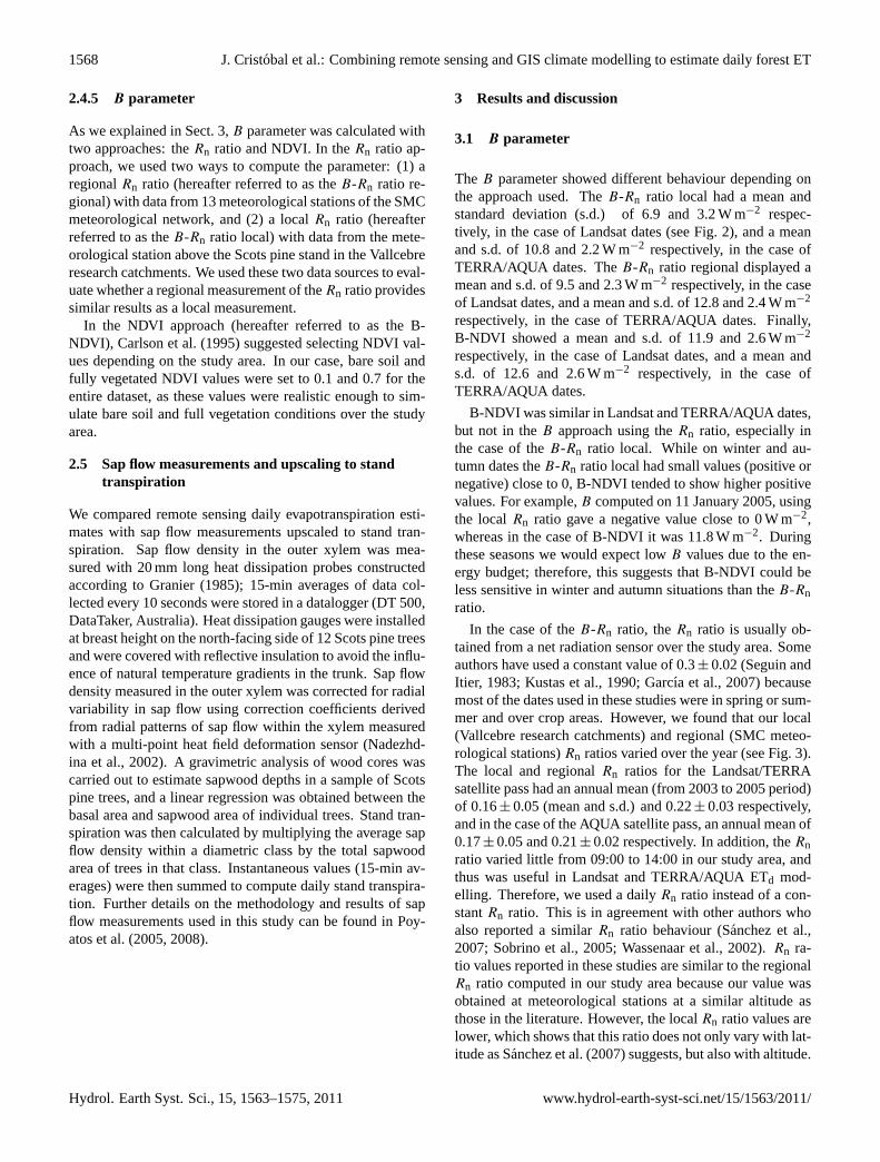
Table 1. (a): Descriptive statistics of daily net radiation (Rnd) and daily evapotranspiration (ETd) measured over the Scots pine stand, andLandsat Rn and ETd modelled using 3 methods:B-Rn ratio regional,B-Rn ratio local and B-NDVI (see text). (b) Model validation results.s.d. is standard deviation, RMSE is root mean square error and MBE is mean bias error.

Rnd Rnd ETd ETd n

measured model measured modelled(W m−2) (W m−2) (mm day−1) (mm day−1)

B-Rn ratio B-NDVI

regional local

Mean 121 106 1.8 2.2 2.0 1.9

17

s.d. 60 62 0.6 0.3 1.0 1.1(a) min 15 9 0.5 0.2 0.0 0.0

max 194 186 2.7 2.1 3.3 3.7

RMSE 22 0.7 0.5 0.6(b) MBE −15 0.4 0.2 0.1

R2 0.89 0.80 0.85 0.85

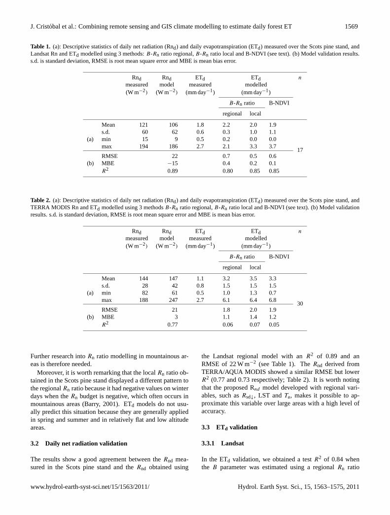
Table 2. (a): Descriptive statistics of daily net radiation (Rnd) and daily evapotranspiration (ETd) measured over the Scots pine stand, andTERRA MODIS Rn and ETd modelled using 3 methodsB-Rn ratio regional,B-Rn ratio local and B-NDVI (see text). (b) Model validationresults. s.d. is standard deviation, RMSE is root mean square error and MBE is mean bias error.

Rnd Rnd ETd ETd n


B-Rn ratio B-NDVI

regional local

Mean 144 147 1.1 3.2 3.5 3.3

30

s.d. 28 42 0.8 1.5 1.5 1.5(a) min 82 61 0.5 1.0 1.3 0.7

max 188 247 2.7 6.1 6.4 6.8

RMSE 21 1.8 2.0 1.9(b) MBE 3 1.1 1.4 1.2

R2 0.77 0.06 0.07 0.05

Further research intoRn ratio modelling in mountainous ar-eas is therefore needed.

Moreover, it is worth remarking that the localRn ratio ob-tained in the Scots pine stand displayed a different pattern tothe regionalRn ratio because it had negative values on winterdays when theRn budget is negative, which often occurs inmountainous areas (Barry, 2001). ETd models do not usu-ally predict this situation because they are generally appliedin spring and summer and in relatively flat and low altitudeareas.

3.2 Daily net radiation validation

The results show a good agreement between theRnd mea-sured in the Scots pine stand and theRnd obtained using

the Landsat regional model with anR2 of 0.89 and anRMSE of 22 W m−2 (see Table 1). TheRnd derived fromTERRA/AQUA MODIS showed a similar RMSE but lowerR2 (0.77 and 0.73 respectively; Table 2). It is worth notingthat the proposed Rnd model developed with regional vari-ables, such asRsd↓, LST andTa, makes it possible to ap-proximate this variable over large areas with a high level ofaccuracy.

3.3 ETd validation

3.3.1 Landsat

In the ETd validation, we obtained a testR2 of 0.84 whenthe B parameter was estimated using a regionalRn ratio



1

Figure 3. Mean monthly local and regional Rn at the Landsat/TERRA and AQUA 2

satellite pass on clear sky days from 2003 to 2005. 3

4

5

Fig. 3. Mean monthly local and regionalRn at the Landsat/TERRAand AQUA satellite pass on clear sky days from 2003 to 2005.

computed with the SMC meteorological stations (B-Rn ratioregional), 0.84 when theB parameter was estimated using alocal Rn ratio computed with the Scots pine stand meteoro-logical station (B-Rn ratio local), and 0.82 when theB pa-rameter was estimated using the NDVI approach, B-NDVI.It is interesting to note that for the ETd models used, the min-imum values were always negative. This mainly happens onwinter dates when theRn ratio is also negative. Therefore, onwinter dates this methodology should only be used on dayswhen theRn budget is positive. Errors close to 1 mm day−1

were obtained for the RMSE. Taking into account the rangeof ETd values observed in the studied Scots pine stand (from0.5 to 2.7 mm day−1), we cannot conclude that the modelprovides optimal results. When theRnd ratio is negative dur-ing winter, the ETd yields negative values and the model doesnot perform well. Again, it is worth noting that ETd modelsare usually validated on spring or summer dates (Chiesi et al.,2002; Nagler et al., 2005, 2007; Sanchez et al., 2007, 2008a;Verstraeten et al., 2005; Wu et al., 2006) when the dailyRnbudget is positive. Our attempt to also estimate ETd duringautumn and winter has shown the limitations of the methodand how ETd modelling needs to be further improved, espe-cially in forest areas.

We obtained a better mean RMSE for the different mod-els when only those dates with a positiveRnd ratio were se-lected, which ranged from 0.5 to 0.7 mm day−1 with a sim-ilar R2 (see Tables 2–3 and Fig. 4). Of the different ap-proaches used to compute theB parameter, the best resultswere obtained using the localRn ratio and the NDVI ap-proaches, with a RMSE of 0.5 and 0.6 mm day−1, respec-tively, and an estimation error of about±30 %. Indeed, theregionalRn ratio yielded a higher RMSE and estimation error

1

Figure 4. Relationship between daily evapotranspiration (ETd) calculated from sap flow 2

measurements modelled using Landsat data and the B parameter approach in mm·day-1

. 3

B-Rn ratio regional is the B approach using the regional Rn ratio, B-Rn ratio local is the 4

B approach using the local Rn ratio and B-NDVI is the B approach using the NDVI. 5

Fig. 4. Relationship between daily evapotranspiration (ETd) cal-culated from sap flow measurements modelled using Landsat dataand theB parameter approach in mm day−1. B-Rn ratio regional istheB approach using the regionalRn ratio,B-Rn ratio local is theB approach using the localRn ratio and B-NDVI is theB approachusing the NDVI.

of about 0.7 mm day−1 and±38 % respectively; this could beexplained by the differences in theRn ratio estimation. TheregionalRn ratio was computed from the data from the SMCmeteorological stations, which are designed for crop assess-ment and are located in areas at low to medium heights (from0 to 500 m). Our study area is located at 1250 m; therefore,the regionalRn ratio conditions are not representative of ourstudy area. However, it is important to note that optimalRnratio values are difficult to obtain because it would be neces-sary to have a meteorological network withRn instrumentsdistributed at different altitudes in diverse landscapes. More-over,Rn instruments are usually found in agrometeorologicalnetworks but not very often over forest areas. Although thetwo B parameter approaches (B-Rn ratio local and B-NDVI)obtained similar results, the main advantage of the NDVI ap-proach is easily implemented, when realistic values of NDVIthresholds to compute NDVI∗ are selected, to compute ETthanB-Rn ratio local or regional because that require inten-sive local calibration. So, if a well-balanced regionalRn ra-tio is not available due to limitations in the meteorologicalnetworks, the NDVI approach is preferable for computingthe B parameter at regional scales in an operative way. Inall cases, the models tended to overestimate ETd, showinghigher values in the case of the regional Rn ratio and lowervalues in the case of the NDVI approach.

In this study, we are strictly comparing evapotranspirationwith stand transpiration of the dominant tree species. As theunderstory in the studied stand is very poor, the only othercontribution comes from soil evaporation, with typical rates



Table 3. (a): Descriptive statistics of daily net radiation (Rnd) and daily evapotranspiration (ETd) measured over the Scots pine stand, andAQUA MODIS Rn and ETd modelled using 3 methods:B-Rn ratio regional,B-Rn ratio local and B-NDVI (see text). (b) Model validationresults. s.d. is standard deviation, RMSE is root mean square error and MBE is mean bias error.

Rnd Rnd ETd ETd n


B-Rn ratio B-NDVI

regional local

Mean 143 148 2.1 3.7 3.9 3.8

27

s.d. 27 41 0.7 1.7 1.6 1.7(a) min 82 62 0.9 1.3 1.6 1.2

max 188 251 3.6 9.0 8.9 8.9

RMSE 22 2.3 2.4 2.3(b) MBE 0 1.6 1.8 1.7

R2 0.73 0.06 0.05 0.03

of 0.1 to 0.5 mm day−1 (Poyatos et al., 2007). These val-ues are consistent with the systematic bias between sap flow-derived transpiration and the ETd models (see Fig. 4).

In addition, it should be stressed that the difficulty of ob-taining the effective aerodynamic resistance and the use of aconstant value for the analyzed period may have introducedmore variability into our analysis, and thus increased the er-ror in the ETd models.

3.3.2 TERRA/AQUA MODIS

TERRA and AQUA ETd validation did not obtain the sameresults as Landsat (see Tables 2–3 and Figs. 5–6). In bothcases, ETd validation showed a higher RMSE, between1.8 and 2.4 mm day−1, a lowR2, between 0.03 and 0.07 andestimation error of about±57 and 50 %, respectively. De-spite air temperature models also showing good validationresults, one possible source of error is the LST. Therefore, itseems that although TERRA/AQUA MODIS LST providesgood results inRnd modelling, this is not the case in ETdmodelling.

The study area does not cover a 1000 m× 1000 m pixel,and therefore the remote sensing data, especially the LST,is less representative than a Landsat pixel of 60 (ETM+) or120 m (TM). As we mentioned in Sect. 2.1, the study area hashigh spatial heterogeneity, mosaic of afforestation patchesovergrowing old agricultural terraces (Poyatos et al., 2003),at smaller scales than the coarse TERRA/AQUA MODISpixel, which makes it difficult to validate the ETd modelresults. However, it has to be noted that validating aTERRA/AQUA MODIS in a heterogeneous mountain land-scape is not easy due to the extensive instrumentation neededto measure the energy flux in each of the landscape covers.Therefore, it seems that the use of TERRA/AQUA MODISimages themselves in this type of landscape is not enough

1

2

Figure 5. Relationship between daily evapotransporation (ETd) calculated from sap flow 3

measurements and modelled using TERRA MODIS data and the B parameter estimation 4

in mm·day-1

. B-Rn ratio regional is the B approach using the regional Rn ratio, B-Rn ratio 5

local is the B approach using the local Rn ratio and B-NDVI is the B approach using the 6

NDVI. 7

Fig. 5. Relationship between daily evapotransporation (ETd)calculated from sap flow measurements and modelled usingTERRA MODIS data and theB parameter estimation inmm·day−1. B-Rn ratio regional is theB approach using the re-gionalRn ratio, B-Rn ratio local is theB approach using the localRn ratio and B-NDVI is theB approach using the NDVI.

to accurately map ET on a daily basis. In order to improvethe ETd results using coarse resolution images, downscalingtechniques such as those in Anderson et al. (2004) are re-quired.

There are very few studies in the literature that moni-tor ETd at both high spatial and temporal resolutions dur-ing an annual period in a forest area, especially using alarge number of Landsat images. In addition, most of thestudies to date have dealt with environments subjected to



1

Figure 6. Relationship between daily evapotransporation (ETd) calculated from sap flow 2

measurements and modelled using AQUA MODIS data and the B parameter estimation 3

in mm·day-1

. B-Rn ratio regional is the B approach using the regional Rn ratio, B-Rn ratio 4

local is the B approach using the local Rn ratio and B-NDVI is the B approach using the 5

NDVI. 6

7

8

9

10

Fig. 6. Relationship between daily evapotransporation (ETd)calculated from sap flow measurements and modelled usingAQUA MODIS data and theB parameter estimation in mm day−1.B-Rn ratio regional is theB approach using the regionalRn ratio,B-Rn ratio local is theB approach using the localRn ratio and B-NDVI is theB approach using the NDVI.

only mild water stress, such as riparian forests, crops orboreal stands. For example, Wu et al. (2006) reported anRMSE of 0.6 mm day−1 in a tropical forest using only oneLandsat image. They compared their results with estimatesfrom the literature due to the difficulty in validating thesekinds of regions using sap flow measurements. Nagler etal. (2005, 2007) modelled ETd using 8 Landsat-5 TM andabout 90 MODIS dates in a cottonwood plantation in ripariancorridors of the western US during the July–August periodin 2005, and obtained an uncertainty in modelled ETd of 20–30 %. Verstraeten et al. (2005) also reported an uncertaintyof about 27 % in instantaneous ET modelled with NOAA-imagery and validated using EUROFLUX data during thegrowing seasons of European forests, from March to Octo-ber. Sanchez et al. (2007) modelled ETd using MODIS in ahomogeneousPinus sylvestrisstand in the boreal region, andreported an RMSE of 0.81 mm day−1 and an uncertainty ofabout 30 % in ETd compared to eddy-covariance data. Witha more demanding method in terms of ancillary data needs,FOREST-BGC, Chiesi et al. (2002) reported a mean RMSEof 0.4 mm day−1 introducing LAI derived from 10-day com-posites of NOAA images in two oak stands. More recently,Sanchez et al. (2008a) obtained a value of 0.7 mm day−1

in different coniferous, broad-leaf and mixed forests in theBasilicata region with three Landsat-5 TM and ETM+ im-ages from spring and summer.

Overall, for Landsat ETd modelling, our results are inagreement with the studies in the literature, as we obtained anuncertainty of about 30 %. One positive point of the results

of the Landsat ETd models across different seasons is the ro-bust ETd estimation under varied conditions of water avail-ability, as the studied stand undergoes different degrees ofwater stress in spring, summer and autumn (Poyatos et al.,2008). However, in the case of MODIS ETd modelling, thevalidation shows a higher RMSE, which suggests that higherspatial resolution is needed for heterogeneous areas.

In addition, it is worth noting that implementing regionalmodels for calculatingTa, LST andRsd↓, as inputs in bothRn and ETd modelling has provided good results and madeit possible to compute these variables at regional scales withsimilar accuracy to that in the literature.

It is important to note, however, that we have found somelimitations in ETd modelling in a mountainous forested areathat should be addressed in the future in order to monitor thisvariable in an operational way. Further work to improve thedescribed methodology should include: (i) the validation ofa multi-scale remote sensing model (Anderson et al., 2004)for disaggregating regional fluxes to micrometeorologicalscales. This would allow ETd to be monitored on a daily ba-sis instead of on a 16-day basis thanks to the TERRA/AQUAtemporal resolution; (ii) the implementation of methodolo-gies for calculating aerodynamic resistance, such as those de-scribed by Norman et al. (1995) and Sanchez et al. (2008a,b).

4 Conclusions

The B-method has been used to estimate daily evapotranspi-ration (ETd) in a Scots pine stand in a mountainous Mediter-ranean area, obtaining an estimation error of±30 % (corre-sponding to 0.5–0.7 mm day−1) using medium spatial reso-lution imagery, Landsat-5 TM and Landsat-7 ETM+, and thedifferent approaches presented. These results are in agree-ment with recent studies that used a similar spatial reso-lution. However, when lower spatial resolution was used(TERRA/AQUA MODIS) the results showed larger errors,1.9 and 1.7 mm day−1 respectively.

TheRn ratio emerged as an important parameter to be con-sidered when the B-method is used. Although this ratio isclose to 0.3 in spring and summer months, this value is notappropriate for winter and autumn because when theRn ra-tio is negative (negativeRn budget) the B-method does notprovide a realistic ETd. Further research is therefore neededto estimate this parameter in these conditions.

The best ETd results were obtained using a localRn ra-tio approach to calculate theB parameter, followed by themethod using NDVI. The regionalRn ratio resulted in largererrors, which means that if a well balanced meteorologicalnetwork (with Rn sensors) is not available, the NDVI ap-proach is preferable for calculating theB parameter at a re-gional scale in an operative way.

Regional input variables for calculating ETd, such asRsd↓,LST andTa, performed well, making possible to compute itat a regional scale with a good level of accuracy.



Finally, using a large number of remote sensing imagesthat are well distributed over the analyzed period, especiallyin the case of Landsat, allowed us to better understand thelimitations of the methodologies and how to address the fur-ther improvement of ETd modelling, especially in forest ar-eas.

Acknowledgements.The authors would like to thank our col-leagues of the Research Group of Methods in Remote Sensingand GIS (GRUMETS) who collaborated in several ways in imagetreatment, and Juan Manuel Sanchez from the Department of EarthPhysics and Thermodynamics of the University of Valencia forhis help in evapotranspiration modelling, and to our colleaguesof the Surface Hydrology and Erosion Group – IDAEA for theirhelp in field data acquisition. It would not have been possible tocarry out this study without the financial support of the Ministryof Science and Innovation and the FEDER funds through theresearch project “SCAITOMI (TIN2009-14426-C02-02)”. TheCatalan Government provided funding to our Research Group forMethods and Applications in Remote Sensing and GeographicInformation Systems – “GRUMETS (2009SGR1511)”, and“MONTES (CSD2008-00040)”. We would like to express ourgratitude to the Catalan Water Agency and to the Ministry ofthe Environment and Housing of the Generalitat (AutonomousGovernment of Catalonia) for their investment policy and theavailability of Remote Sensing data, which has made it possibleto conduct this study under optimal conditions. Xavier Pons isrecipient of an ICREA Academia Excellence in Research grant.

Edited by: J. Liu

References

Allen, R. G., Pereira, L. S., Raes, D., and Smith, M.: Crop evapo-transpiration, Guidelines for computing crop water requeriments,FAO Irrigation and Drainage Paper, 56, 1998.

Allen, R. G., Tasumi, M., and Trezza, R.: Satellite-based energybalance for mapping evapotranspiration with internalized cali-bration (METRIC)-Model, J. Irrig. and Drain. E.-ASCE, 133,395–406, 2007.

Anderson, M. C., Norman, J. M., Mecikalski, J. R., Torn, R. D.,Kustas, W. P., and Basara, J. B.: A multi-scale remote sensingmodel for disaggregating regional fluxes to micrometeorologicalscales, J. Hydrometeorol., 5, 343–363, 2004.

Baldasano, J. M., Calbo, J., and Moreno J.: Atlas de Radiacio Solara Catalunya (Dades del perıode 1964–1993), Institut de Tecnolo-gia i Modelitzacio Ambiental (ITEMA), Universitat Politecnicade Catalunya, Terrassa, 1994.

Barry, R. E.: Mountain weather and climate, 2nd edition, Rout-ledge, Taylor and Francis Group, London, 2001.

Bastiaanssen, W. G. M., Meneti, M., Feddes, R. A., and Holtslag,A. A. M.: A remote sensing surface energy balance algorithm forland (SEBAL), 1. Formulation, J. Hydrol., 212–213, 198–212,1998.

Bates, B. C., Kundzewicz, Z. W., Wu, S., and Palutikof, J. P.: Cli-mate Change and Water, Technical Paper of the Intergovernmen-tal Panel on Climate Change, IPCC Secretariat, Geneva, 2008.

Carlson, T. N. and Buffum, M. J.: On Estimating Total Daffy Evap-otranspiration from Remote Surface Temperature Measurements,Remote Sens. Environ., 29, 197–207, 1989.

Carlson, T. N., Caphart, J., and Gillies, R. R.: A new look at thesimplified method for remote sensing of daily evapotranspiration,Remote Sens. Environ., 54, 161–167, 1995.

Caselles, V., Sobrino, J. A., and Coll, C.: On the use of satellite ther-mal data for determining evapotranspiration in patially vegetatedareas, Int. J. Remote Sens., 13, 2669–2682, 1992.

Caselles, V., Artiago, M. M., and Hurtado, E.: Maping actual evap-otranspiration by combining Landsat and NOAA-AVHRR im-ages: application to the Barrax area, Albacete, Spain, RemoteSens. Environ., 63, 1–10, 1998.

Chander, G., Markham, B. L., and Helder, D. L.: Summary of cur-rent radiometric calibration coefficients for Landsat MSS, TM,ETM+, and EO-1 ALI sensors, Remote Sens. Environ., 113,893–903, 2009.

Chiesi, M., Maselli, F., Bindi, M., Fibbi, L., Bonora, L., Raschi,A., Tognetti, R., Cermak, J., and Nadezhdina, N.: Calibrationand application of FOREST-BGC in a Mediterranean area by theuse of conventional and remote sensing data, Ecol. Model., 154,251–262, 2002.

Cristobal, J., Pons, X., and Serra, P.: Sobre el uso operativo deLandsat-7 ETM+ en Europa, Revista de Teledeteccion, 21, 55–59, 2004.

Cristobal, J., Pons, X., and Ninyerola, M.: Modelling Actual Evap-otranspiration in Catalonia (Spain) by means of Remote Sensingand Geographical Information Systems, Gottinger Geographis-che Abhandlungen, 113, 144–150, 2005.

Cristobal, J., Ninyerola, M., and Pons, X.: Modelling air tempera-ture through a combination of Remote Sensing and GIS data, J.Geophys. Res., 13, D13106,doi:10.1029/2007JD009318, 2008.

Cristobal, J., Jimenez-Munoz, J. C., Sobrino, J. A., Ninyerola,M., and Pons, X.: Improvements in land surface tempera-ture retrieval from the landsat series thermal band using wa-ter vapour and air temperature, J. Geophys. Res., 114, D08103,doi:10.1029/2008JD010616, 2009.

Dilley, A. C. and O’Brien, D. M.: Estimating downward clear skylong-wave irradiance at the surface from screen temperature andprecipitable water, Q. J. Roy. Meteorol. Soc., 124, 1391–1401,1998.

Gallart, F., Llorens, P., Latron, J., and Regues, D.: Hydrologicalprocesses and their seasonal controls in a small Mediterraneanmountain catchment in the Pyrenees, Hydrol. Earth Syst. Sci., 6,527–537,doi:10.5194/hess-6-527-2002, 2002.

Gallart, F., Latron, J., and Llorens, P.: Catchment dynamics ina Mediterranean mountain environment: the Vallcebre researchbasins (South Eastern Pyrenees), I: Hydrolog, in: Catchment Dy-namics and River Processes: Mediterranean and Other ClimateRegions, edited by: Garcia, C. and Batalla, R., Elsevier, Amster-dam, The Netherlands, 1-16, 2005.

Garcıa, M., Villagarcıa, L., Contreras, S., Domingo, F., andPuigdefabregas, J.: Comparison of Three Operative Models forEstimating the Surface Water Deficit using ASTER Reflectiveand Thermal Data, Sensors, 7, 860–883, 2007.

Granier, A.: Une nouvelle methode pur la mesure du flux de sevebrute dans le tronc des arbres, Ann. Sci. Fores., 42, 193–200,1985.


http://dx.doi.org/10.1029/2007JD009318

http://dx.doi.org/10.1029/2008JD010616

http://dx.doi.org/10.5194/hess-6-527-2002


Hargreaves, G. H. and Samani, Z. A.: Estimating potential evapo-transpiration. ASCE, J. Irrig. Drain. Div., 108, 225–230, 1982.

Jackson, R. D., Reginato, R. J., and Idso, S. B.: Wheat canopytemperature: a practical tool for evaluating water requirements,Water Resour. Res., 13, 651–656, 1977.

Jackson, R. B., Carpenter, S. R., Dahm, C. N., McKnight, D. M.,Naiman, R. J., Postel, S. L., and Running, S. W.: Water in achanging world, Ecol. Appl., 11, 1027–1045, 2001.

Jung, M., Reichstein, M., Ciais, P., Seneviratne, S. I., Sheffield,J., Goulden, M. L., Bonan, G., Cescatti, A., Chen, J., Jeu, R.,Dolman, A. J., Eugster, W., Gerten, D., Gianelle, D., Gobron,N., Heinke, J., Kimball, J., Law, B. E., Montagnani, L., Mu,Q., Mueller, B., Oleson, K., Papale, D., Richardson, A. D.,Roupsard, O., Running, S., Tomelleri, E., Viovy, N., Weber, U.,Williams, C., Wood, E., Zaehle, S., and Zhang, K.: Recent de-cline in the global land evapotranspiration trend due to limitedmoisture supply, Nature, 467, 951–954, 2010.

Kustas, W. P. and Norman, J. M.: Use of remote sensing for evap-otranspiration monitoring over land surfaces, Hydrolog. Sci. J.,41, 495–516, 1996.

Kustas, W. P. and Norman, J. M.: A two-source energy balanceapproach using directional radiometric temperature observationsfor sparse canopy covered surfaces, Agron. J., 92, 847–854,2000.

Kustas, W. P., Moran, M. S., Jackson, R. D., Gay, L. W., Duell,L. F. W., Kunkel, K. E., and Matthias, A. D.: Instantaneous anddaily values of the surface energy balance over agricultural fieldsusing remote sensing and reference field in an arid environment,Remote Sens. Environ, 32, 125–141, 1990.

Lagouarde, J. P. and Brunet, Y.: A simple model for estimatingthe daily upward longwave surface radiation flux from NOAA-AVHRR data, Int. J. Remote Sens., 14, 907–925, 1983.

Latron, J., Llorens, P., Soler, M., Poyatos, R., Rubio, C., Muzylo,A., Martınez-Carreras, N., Delgado, J., Regues, D., Catari, G.,Nord, G., and Gallart, F.: Hydrology in a Mediterranean moun-tain environment – the Vallcebre research basins (northeasternSpain). I. 20 years of investigations of hydrological dynamics,in: Status and Perspectives of Hydrology in Small Basins, IAHSPubl. 336, IAHS Press, Wallingford, UK, 38–44, 2010.

Liang, S.: Narrowband to broadband conversions of land surfacealbedo, Remote Sens. Environ., 76, 213–238, 2001.

Liang, S., Strahler, A. H., and Walthall, C.: Retrieval of land surfacealbedo from satellite observations: a simulation study, J. Appl.Meteorol., 38, 712–725, 1999.

Liu, J., Williams, J. R., Zehnder, A. J. B., and Yang, H.: GEPIC– modelling wheat yield and crop water productivity with highresolution on a global scale, Agr. Syst., 94, 478–493, 2007.

Liu, J., Zehnder, A. J. B., and Yang, H.: Global consump-tive water use for crop production: The importance of greenwater and virtual water, Water Resour. Res., 45, W05428,doi:10.1029/2007WR006051, 2009.

Llorens, P., Poyatos, R., Muzylo, A., Rubio, C., Latron, J., Del-gado, J., and Gallart, F.: Hydrology in a Mediterranean moun-tain environment – the Vallcebre research basins (northeasternSpain), III. Vegetation and water fluxes, in: Status and Per-spectives of Hydrology in Small Basins, IAHS Publ. 336, IAHSPress, Wallingford, UK, 186–191, 2010.

Mu, Q., Heinsch, F. A., Zhao, M., and Running, S. W.: Develop-ment of a global evapotranspiration algorithm based on MODISand global meteorology data, Remote Sens. Environ., 111, 519–536, 2007.

Nadezhdina, N.,Eermak, J., and Ceulemans, R.: Radial patternsof sap flow in woody stems of dominant and understory species:scaling errors associated with positioning of sensors, Tree Phys-iol., 22, 907–918, 2002.

Nagler, P., Cleverly, J., Glenn, E., Lampkin, D., Huete, A., and Wan,Z.: Predicting riparian evapotranspiration from MODIS vegeta-tion indices and meteorological data, Remote Sens. Environ., 94,17–30, 2005.

Nagler, P., Jetton, A., Fleming, J., Didan, K., Glenn, E., Erker, J.,Morino, K., Milliken, J., and Gloss, S.: Evapotranspiration ina cottonwood (Populus frmontii) restoration plantation estimatedby sap flow and remote sensing methods, Agr. Forest Meteorol.,144, 95–110, 2007.

Ninyerola, M., Pons, X., and Roure, J. M.: A methodological ap-proach of climatological modelling of air temperature and pre-cipitation through GIS techniques, Int. J. Climatol., 20, 1823–1841, 2000.

Ninyerola, M., Pons, X., and Roure, J. M.: Objective air tempera-ture mapping for the Iberian Peninsula using spatial interpolationand GIS, Int. J. Climatol., 27(9), 1231–1242, 2007.

Norman, J. M., Kustas, W. P., and Humes, K.: A two-source ap-proach for estimating soil and vegetation energy fluxes from ob-servations of directional radiometric surface temperature, Agr.Forest Meteorol., 77, 263–293, 1995.

ORNL DAAC – Oak Ridge National Laboratory Distributed ActiveArchive Center: SAFARI 2000 Web Page,http://daac.ornl.gov/S2K/safari.html, last access: 1 September, 2010.

Oki, T. and Kanae, S.: Global Hydrological Cycles and World Wa-ter Resources, Science, 313, 1068–1072, 2006.

Page, J. K.: Prediction of solar radiation on inclined surfaces, Solarenergy, R & D in the European Community, Series F: Solar Ra-diation Data, 3, Reidel Publishing Company, Dordrecht, 1986.

Pala, V. and Pons, X.: Incorporation of relief into geometric cor-rections based on polynomials, Photogramm. Eng. Rem. S., 61,935–944, 1995.

Pons, X. and Ninyerola, M.: Mapping a topographic global solarradiation model implemented in a GIS and refined with grounddata, Int. J. Climatol., 28, 1821–1834, 2008.

Pons, X. and Sole-Sugranes, L.: A Simple Radiometric CorrectionModel to Improve Automatic Mapping of Vegetation from Mul-tispectral Satellite Data, Remote Sens. Environ., 47, 1–14, 1994.

Poyatos, R., Latron, J., and Llorens, P.: Land-Use and Land-Coverchange after agricultural abandonment, The case of a Mediter-ranean Mountain Area (Catalan Pre-Pyrenees), Mt. Res. Dev.,23, 52–58, 2003.

Poyatos, R., Llorens, P., and Gallart, F.: Transpiration of montanePinus sylvestris L. and Quercus pubescens Willd. forest standsmeasured with sap flow sensors in NE Spain, Hydrol. Earth Syst.Sci., 9, 493–505,doi:10.5194/hess-9-493-2005, 2005.

Poyatos, R., Villagarcıa, L., Domingo, F., Pinol, J., and Llorens,P.: Modelling evapotranspiration in a Scots pine stand underMediterranean mountain climate using the GLUE methodology,Agr. Forest Meteorol., 146, 13–28, 2007.


http://dx.doi.org/10.1029/2007WR006051

http://daac.ornl.gov/S2K/safari.html

http://daac.ornl.gov/S2K/safari.html

http://dx.doi.org/10.5194/hess-9-493-2005


Poyatos, R., Llorens, P., Pinol, J., and Rubio, C.,: Response of Scotspine (Pinus sylvestris L.) and pubescent oak (Quercus pubescensWilld.) to soil and atmospheric water deficits under Mediter-ranean mountain climate, Ann. Forest Sci., 65, 306, 2008.

Roerink, G. J., Su, Z., and Menenti, M.: S-SEBI: A simple remotesensing algorithm to estimate the surface energy balance, Phys.Chem. Earth Pt. B, 25, 147–157, 2000.

Rost, S., Gerten, D., Bondeau, A., Lucht, W., Rohwer, J., andSchaphoff, S.: Agricultural green and blue water consumptionand its influence on the global water system, Water Resour. Res.,44, W09405,doi:10.1029/2007WR006331, 2008.

Sanchez, J. M., Caselles, V., Niclos, R., Valor, E., Coll, C., andLaurila, T.: Evaluation of the B-method for determining actualevapotranspiration in a boreal forest from MODIS data, Int. J.Remote Sens., 27, 1231–1250, 2007.

Sanchez, J. M., Scavone, G., Caselles, V., Valor, E., Copertino, V.A., and Telesca, V.: Monitoring daily evapotranspiration at a re-gional scale from Landsat-TM and ETM+ data: Application tothe Basilicata region, J. Hydrol., 351, 58–70, 2008a.

Sanchez, J. M., Kustas, W. P., Caselles, V., and Anderson, M. C.:Modelling surface energy fluxes over maize using a two-sourcepatch model and radiometric soil and canopy temperature obser-vations, Remote Sens. Environ., 112, 1130–1143, 2008b.

Schmugge, T. J., Kustas, W. P., Ritchie, J. C., Jackson, T. J., andRango, A.: Remote sensing in hydrology, Adv. Water Resour.,25, 1367–1385, 2002.

Seguin, B. and Itier, B.: Using midday surface temperature to es-timate daily evapotranspiration from satellite IR data, Int. J. Re-mote Sens., 4, 371–383, 1983.

Siebert, S. and Doll, P.: Quantifying blue and green virtual watercontents in global crop production as well as potential productionlosses without irrigation, J. Hydrol., 384, 198–217, 2010.

Sobrino, J. A. and Raissouni, N.: Toward remote sensing methodsfor land conver dynamic monitoring: application to Moroco, Int.J. Remote Sens., 21, 353–366, 2000.

Sobrino, J. A., Gomez, M., Jimenez-Munoz, J. C., Olioso, A., andChehbouni, G.: A simple algorithm to estimate evapotranspira-tion from DAIS data: Application to the DAISEX campaigns, J.Hydrol., 315, 117–125, 2005.

Sobrino, J. A., Jimenez-Munoz, J. C., Soria, G., Romaguera, M.,Guanter, L., Moreno, J., Plaza, A., and Martınez, P.: Land sur-face emissivity retrieval from different VNIR and TIR sensors,IEEE T. Geosci. Remote, 46, 316–327, 2008.

Verstraeten, W. W., Veroustraete, F., and Feyen, J.: Estimatingevapotranspiration of European forests from NOAA-imagery atsatellite overpass time: Towards an operational processing chainfor integrated optical and thermal sensor data products, RemoteSens. Environ., 96, 256–276, 2005.

Vidal, A. and Perrier, A.: Analysis of a simplified relation for es-timating daily evapotranspiration from satellite thermal IR data,Int. J. Remote Sens., 10, 1327–1337, 1989.

Wassenaar, T., Olioso, A., Haseger, C., Jacob, F., and Chehbouni,A.: Estimation of evapotranspiration on heterogeneous pixels,edited by: Sobrino, A. J. A., First International Symposiumon Recent Advances in Quantitative Remote Sensing, Valencia,Spain, Publicacions de la Universitat de Valencia, 2002.

Wu, W., Hall, C. A. S., Scatena, F. N., and Quackenbush, L. J.: Spa-tial modelling of evapotranspiration in the Luquillo experimentalforest of Puerto Rico using remotely-sensed data, J. Hydrol., 328,733–752, 2006.


http://dx.doi.org/10.1029/2007WR006331

combining remote sensing and gis climate modelling to

Documents