color glass condensate inspired scaling and gluon saturation

UNIVERSITY OF BUCHAREST

FACULTY OF PHYSICS

MASTER THESIS

Color Glass Condensate Inspired Scalingand Gluon Saturation

Amelia LINDNER

Supervisors:Prof. Dr. Mihai PETROVICI

Prof. Dr. Alexandru JIPA

Hadronic Physics Department (HPD)Horia Hulubei National Institute for R&D in Physics and Nuclear Engineering

(IFIN-HH)

June 2019

Abstract

The latest experimental results from RHIC and LHC are used in this thesis in orderto study the dependence of different observables on the square root of the hadronmultiplicity over unit of rapidity and unit of transverse overlapping area, the ColorGlass Condensate inspired scaling variable. The most relevant dependencies on thisgeometrical variable, like the < pT >, the slopes of < pT > - mass dependence andthe Boltzmann-Gibbs Blast Wave fit parameters will be discussed.

This study was conducted for a large range of energies, from 7.7 GeV, up to 5.44TeV, for several colliding systems, i.e. Cu-Cu, Au-Au, Pb-Pb and Xe-Xe, based onpublished experimental data and Glauber Monte Carlo estimates. Signs of gluonsaturation are present for the most central collisions for the highest center-of-massenergies available at LHC.

Similarities between small colliding systems (pp) and heavy ion collisions (Pb-Pb) at LHC energies are also reported in this thesis.

iii

Acknowledgements

I would like to express my deepest gratitude to my Supervisor, Prof. Dr. MihaiPetrovici, for his professional guidance, immense knowledge, but most important,for inspiring me with his work ethic and infinite enthusiasm. Furthermore, I wouldlike to thank him for providing me the possibility to work in an incredible researchenvironment, that can only encourage and inspire a young scientist like me.

Further thanks to Dr. Amalia Pop, Dr. Cristian Andrei and Dr. Andrei Herghelegiufor their guidance, suggestions, for their patience and fruitful discussions.

I would also like to express my thanks for all the people in the Hadron PhysicsDepartment.

v

Contents

Abstract iii

1 Introduction 11.1 Quantum Chromodynamics . . . . . . . . . . . . . . . . . . . . . . . . . 1

1.1.1 Asymptotic Freedom . . . . . . . . . . . . . . . . . . . . . . . . . 21.2 The Phase Diagram of Strongly Interacting Matter . . . . . . . . . . . . 31.3 Deep Inelastic Scattering . . . . . . . . . . . . . . . . . . . . . . . . . . . 51.4 Color Glass Condensate . . . . . . . . . . . . . . . . . . . . . . . . . . . 6

2 Heavy Ion Collisions 92.1 High Energy Density versus High Baryon Density . . . . . . . . . . . . 92.2 The Geometry of a Collision and the Glauber Model . . . . . . . . . . . 102.3 The Core-Corona Effect . . . . . . . . . . . . . . . . . . . . . . . . . . . . 132.4 Review of the Main Results Obtained at RHIC and LHC . . . . . . . . 16

2.4.1 Au-Au Collisions at RHIC:√

sNN = 62.4, 130 and 200 GeV . . . 162.4.2 Au-Au Collisions at RHIC: Beam Energy Scan Program . . . . . 172.4.3 Pb-Pb & Xe-Xe Collisions at LHC . . . . . . . . . . . . . . . . . . 19

3 Proton-Proton Collisions at LHC Energies 233.1 The Geometry of pp Collisions . . . . . . . . . . . . . . . . . . . . . . . 233.2 Parton Density and Occupation Number in pp Collisions . . . . . . . . 253.3 Review of the Main Results Obtained at LHC in Small Systems and

Similarities between pp, p-Pb and Pb-Pb Collisions . . . . . . . . . . . 26

4 Color Glass Condensate Scaling Variable 294.1 Expectations of < pT > Behavior as a Function of Collision Energy

and Centrality . . . . . . . . . . . . . . . . . . . . . . . . . . . . . . . . . 294.2 dN/dy Estimates . . . . . . . . . . . . . . . . . . . . . . . . . . . . . . . 304.3 S⊥ Estimates for A-A Collisions . . . . . . . . . . . . . . . . . . . . . . . 314.4 S⊥ Estimates for pp Collisions . . . . . . . . . . . . . . . . . . . . . . . . 32

5 Results 355.1 Systematic Study of the

√sNN Dependence . . . . . . . . . . . . . . . . 35

5.1.1 < pT > as a function of√( dN

dy )/Sgeom⊥ . . . . . . . . . . . . . . . 35

Core-Corona Interplay . . . . . . . . . . . . . . . . . . . . . . . . 37

5.1.2 < pT > mass dependence as a function of√( dN

dy )/Sgeom⊥ . . . . 39

vii

5.1.3√( dN

dy )/Sgeom⊥ dependence of Boltzmann-Gibbs Blast Wave Fit

parameters . . . . . . . . . . . . . . . . . . . . . . . . . . . . . . . 415.2 Systematic Study of the System Size Dependence . . . . . . . . . . . . . 45

5.2.1 Heavy Ion Collisions . . . . . . . . . . . . . . . . . . . . . . . . . 455.2.2 Small systems (pp) versus heavy systems (Pb-Pb) at LHC en-

ergies . . . . . . . . . . . . . . . . . . . . . . . . . . . . . . . . . . 46

6 Summary and Outlook 49

viii

1 | Introduction

High energy heavy ion collisions are the only way to recreate in the laboratory thestates of matter supposed to be existing a few microseconds after the Big Bang, interms of densities and temperatures. In understanding the phenomena producedcolliding two heavy ions, one has to consider that the matter will present some finitesize effects, it has a violent evolution in time and highly non-homogenous in itsinitial state. All these have to be considered and be taken into account when theproperties of this kind of matter are studied.

The Introduction chapter contains the theoretical framework of this thesis, start-ing with a short description of the Quantum Chromodynamics (QCD) theory, itsproperties, the description of the phase diagram of strongly interacting matter andending with the limitations of the perturbative QCD (pQCD) and a short descriptionof a theoretical model that works in the non-perturbative regime of QCD, the ColorGlass Condensate (CGC).

Arguments for studying heavy ion collisions are summarized in the second chap-ter. Some basic notions about the collision geometry and of the model that describesthe heavy ion collisions from the geometrical point of view, i.e. Glauber model, themain research facilities in the heavy ion collisions field and some of the results ob-tained at RHIC (Relativistic Heavy Ion Collider) and LHC (Large Hadron Collider)are presented. The fourth chapter contains a description of the proton-proton (pp)collisions, considered a very good benchmark for the heavy ion collisions and whyare they relevant at the energies reached at LHC. The similarities with heavy ioncollisions, are also discussed in this chapter.

In the fifth chapter chapter is introduced the scaling variable inspired by theCGC model and how it was obtained for several colliding systems and center ofmass energies that were used in this study. In the sixth chapter are presented theresults of the present study and their significance. A summary and the outlook ofthis thesis are presented in the seventh chapter.

1.1 Quantum Chromodynamics

The evolution of experimental particle physics has lead to the discovery of quarks, asthe fundamental particles that form all the existing hadrons. The hadrons are com-posed of three quarks, in the case of baryons, or two quarks, in the case of mesons.The quarks are interacting to each other through the strong force. The particularitythat quarks possess in order to be able to participate in the strong interaction is thatthey are carrying color charges.

1

Chapter 1. Introduction

The quarks interact to each other through bosons that are mediating the stronginteraction, which are called gluons, also carrying color charges. This particularityof gluons leads to the fact that they are able to interact with each other, resultingsome interesting features that the strong interaction possesses, that will be discussedbelow.

The field theory of strong interactions is known as Quantum Chromodynamics(QCD), which describes the fields of quarks and gluons and their interactions.

The QCD Lagrangian density is [1]:

LQCD = ∑f

q fi (x)(iγµDµ −m f )ijq

fj (x)− 1

4Fa

µνFµνa (1.1)

where q fi and qi

f are used for the notations of quark and antiquark (spin -1/2 Dirac),fields of color i,j (red, green, blue), flavour f (up, down, strange, charm, bottom, top)and their associated masses.

The covariant derivative, Dµ is defined by:

Dµ = ∂µ − igAµ (1.2)

Faµν = ∂µ Aa

ν − ∂ν Aaµ + g f abc Ab

µ Acν (1.3)

where Aaµ are the gluon fields (the spin 1 boson with zero mass and color a), Fa

µν isthe non-Abelian gluon field strength tensor, f abc are the structure constants of thecolor group SU(3) and µ2 is the energy scale of the process which has an arbitraryvalue, so it could be equal with the squared four-momentum transfer, Q2.

1.1.1 Asymptotic Freedom

Experimentally was evidenced that as the quarks within a hadron are getting closerto each other, the strong coupling between them asymptotically approaches zero atshort distances, which implies a large momentum transfer. This leads to the phe-nomenon called asymptotic freedom at high momentum transfer and, in the case ofa low momentum transfer, to a strong coupling regime. This effect tells us that thequarks inside a hadron behave more or less as free particles, depending on the theamount of momentum transfer (Fig. 1.1).

The running coupling constant is [1]:

αs(Q2) =αs(µ2)

1 + αs(µ2)β2ln(Q2

µ2 )(1.4)

where

β2 =11Nc − 2N f

12π(1.5)

and Nc is the number of colors, while N f stands for the number of quark flavours.The behavior of quarks and gluons at large momenta is clear from Eq.1.4, where

one can see that αs → 0 as Q2 → ∞, which shows that the quarks and gluons areinteracting weakly at short distances.

2

1.2. The Phase Diagram of Strongly Interacting Matter

FIGURE 1.1: The running coupling constant, αs, as a function of theenergy scale, Q, and the comparison between experimental data and

the theoretical predictions [2].

Due to the asymptotic freedom phenomenon, one can use the perturbation the-ory for the case of a large momentum transfer, where the perturbative QCD (pQCD)explains rather good the experimental data.

The region where the values of the coupling constant is small enough in orderto treat the strong interaction in the perturbative regime is set by the fundamentalscale of QCD, ΛQCD. The coupling constant of QCD has the following dependence ofΛQCD [1]:

αs(Q2) =2π

β0ln(Q2/ΛQCD)(1.6)

whereΛQCD ∼ 200MeV (1.7)

The notions of light and heavy quarks are also defined relative to ΛQCD. Oneconsiders the light quarks those flavours with masses much smaller than ΛQCD (up,down), while the heavy quarks are those with masses larger than ΛQCD (charm,bottom, top), the strange quark being an exception, in some cases being treated aslight and in others as a heavy quark.

1.2 The Phase Diagram of Strongly Interacting Matter

The thermodynamic properties of a system are expressed in terms of a phase dia-gram that illustrates the mutual dependence of the thermodynamic parameters of

3

the system. In the case of QCD, the phase diagram is expressed in terms of thetemperature, T, as a function of the baryonic chemical potential, µB. Each point ofthe QCD phase diagram corresponds to a stable thermodynamic state, which is de-scribed by specific thermodynamic functions (Fig. 1.2).

Due to the phenomenon of asymptotic freedom of QCD, the phases of QCDthat involve high temperatures and high baryonic chemical potentials are better de-scribed in terms of quarks and gluons as degrees of freedom.

FIGURE 1.2: The phase diagram of QCD [3].

In the first tens of microseconds after the Big Bang, the only part of the phasediagram reached was the zero baryon number density region, as the Universe wascooling down. In this region, QCD lattice simulations can be performed.

The phase transition between the hadronic gas and the matter deconfined in itsconstituents, quarks and gluons, the so-called partons, has a critical point, charac-terised by the critical temperature, Tc. In the approximation of two massless quarks,where mu = md = 0 and ms is very large (the chiral limit), the phase transition is oneof the second order and for temperatures T < Tc, the chiral symmetry is broken byquark masses, while for T > Tc, the chiral symmetry is restored. Since in naturethe quarks are not massless, the second order phase transition is considered to bea crossover region for µB = 0. Also, in the case where ms has a comparable valueto those of the up and down quarks, the phase transition is predicted by the latticesimulations to be a first order transition [4].

Another interesting region of the phase diagram, the region described by highbaryonic density matter at low temperatures, dense enough so that it cannot be madeof individual well-separated nucleons, even at low temperatures, is supposed to becharacteristic for the center of a neutron star. At even lower temperatures and higherdensities, i.e. higher baryonic chemical potential, theoretical models predict a newregime of color superconducting quark matter.

4

1.3. Deep Inelastic Scattering

1.3 Deep Inelastic Scattering

Since the discovery of quarks and gluons as fundamental particles, the next stepwas the investigation of the structure of the proton, based on high energy scatteringprocesses.

There are two types of scattering processes in QCD, characterised by the frac-tion of the momentum exchange in the scattering between probe and the constituentpartons of the initial hadron, x. The soft interactions are those which correspond tox 1 and are non-perturbative processes with large cross sections, while the hardinteractions are characterised by x ∼ 1, such as jets, with small cross sections, butbecause of the asymptotic freedom of QCD, these kind of processes can be treatedby pQCD. Since hard interactions are very rare processes, due to the fact that canhappen only when in the initial state of the hadron appear in some rare fluctuations,the soft processes provide a very high interest in the field of QCD.

Deep inelastic scatterings (DIS) are semihard processes, where only a small amountof energy is exchanged between the probe and hadron’s constituents. The semihardprocesses are providing valuable information because they have cross sections com-parable to the size of a hadron, but unlike the soft interactions, this process appearsat small transverse distances, so one can observe the physics related to soft interac-tions in this semihard processes, while the amplitudes of these interactions can be

FIGURE 1.3: The contribution of each flavour into the partonic distri-bution functions of a proton, measured in deep inelastic scattering, at

HERA [5].

5


calculated with pQCD.The study of deep inelastic scatterings of different charged or neutral leptons on

nucleons or nuclear targets have lead to the determination of the parton distributionsfunctions (PDFs), obtained by fitting the experimental data. Since QCD doesn’t pre-dict the parton distributions inside a proton. The electron-proton collider at HERAwas opening a new landscape, by reaching large range in x and Q2 [6].

Some of the experimental results obtained at HERA are summarized in Fig. 1.3,in terms of PDFs of a proton at Q2 = 10 GeV2, separated into the contribution of eachflavour, obtained from the fit parametrisations of the PDFs, which are the gluondistributions (xg), the valence quark distributions (xuv and xdv) and the sea quarkpairs distributions (xS), which are the main constituents of a hadron, in the infinitemomentum frame, described by the parton model, in the Bjorken limit.

1.4 Color Glass Condensate

One can observe in Fig. 1.3 that the gluon distribution of a proton rises very fast withdecreasing x. The stability of the parton model consists in the maximum occupationnumber of the gluons to have an 1/αs order where we have a saturation scale, Qs(x),that increases as x decreases. In this limit, the proton can be considered a dense manybody system of gluons (Fig. 1.4). In the Regge-Gribov limit (Q2 - fixed, x→ 0), thehadron structures can be observed for Q2 ≥ 1 GeV2.

Color Glass Condensate (CGC) is an effective field theory where the degrees offreedom are separated into fast frozen color sources and slow dynamical color fields,

FIGURE 1.4: The phase diagram of the QCD evolution [7].

6

1.4. Color Glass Condensate

which describes the properties of matter where gluon saturation is present. Thename can be very well understood by analysing it word by word: color - the modeldescribes a state of matter made of gluons with colors, glass - the gluons are evolvingon much longer time scales than the natural time scale, 1/Qs, combined with thestochastic nature of sources, and condensate - the high density of matter, which has alarge occupation number of gluons.

The CGC framework is an important tool because it describes the collective dy-namics of QCD at high densities of partons. This model proves the universality ofthe physics of saturated gluons and shows that it is independent of the fragmenta-tion region, based on the high similarity between protons and heavy nuclei, for thesame values of the impact parameter, at high energies. Also, it can describe a widevariety of processes, like e+p, e+A, p+A or A+A collisions.

The motivation of using this CGC model is for understanding the soft QCD dy-namics. The CGC is giving an approach in order to study thermalization in heavyion collisions and also the initial conditions that are standing for the evolution of thethermalized deconfined matter.

7

2 | Heavy Ion Collisions

Heavy ion collisions represent one of hottest topics of nowadays and the last half ofcentury, with an impressive evolution in both theory and experiments. In the lastdecades, as soon as ultrarelativistic beams of several types of nuclei or protons be-came available, the physics beyond these collisions was studied intensively. Withoutthe remarkable progresses in this field of research, the dynamical phenomena or theunderstanding of the properties of matter described by QCD would have been neg-ligible, due to the strength of the QCD interactions that can’t be studied in any otherway.

The study of heavy ion collisions gives us the opportunity to have an insight ofthe mechanisms the particle production in these high energy collisions, where thereare still some unanswered questions that date back even before the development ofQCD. Initially, the need of heavy ion experiments came with the understanding thatthe matter that was filling up the universe a few microseconds after the Big Banghad temperatures higher than ΛQCD, so any kind of hadrons were impossible to beproduced, the main goal of heavy ion collision experiments being the recreation,in the laboratory, of droplets of this kind of matter. The possibility to recreate thisBig Bang characteristic type of matter is giving us the only chance to explore itsproperties, dynamics, and the phase diagram of QCD.

2.1 High Energy Density versus High Baryon Density

The study of the QCD’s phase diagram and the search of its critical point (whoseexistence was predicted by several theoretical models) are the main goal of heavy ionexperiments. The phase diagram is studied in heavy ion collisions at both RHIC andLHC experimental facilities where beams of different types of nuclei are collided, byvarying the collision energies, thus the T and µB parameters that are describing it(Fig. 1.2).

The highest center of masses energies in these collisions are reached at LHC,where is explored the free baryonic region of the phase diagram, i.e. µB ≈ 0 andhigh temperatures, where the predictions of the lattice QCD calculations of reachhigh energy densities can be verified. The maximum values of the energy density isreached when the two Lorentz contracted nuclei collide. The Lorentz contraction isdescribed by the γ factor, which increases with the center of mass energy. At LHCthe reached energy density values are 20 times higher than inside a hadron. Suchstate of matter, called Glasma [8] is highly coherent and makes the transition fromCGC to Quark Gluon Plasma (QGP).The initial longitudinal flux tubes of electric and

9

Chapter 2. Heavy Ion Collisions

magnetic color fields expand outwards, inducing transverse fields strengths decay-ing into particles. The partons are strongly coupled to each other, forming a state ofdeconfined matter where they move collectively, a medium that behaves like a rel-ativistic fluid that flows hydrodynamically, whose motion, expansion and coolingdepend on its initial high pressure. This state of deconfined matter holds for as longas the energy density in all its volume stays above to that of an individual hadron.

Since this high energy density is not reached in all the volume of the collidingnuclei, there are parts of the initial colliding nuclei that are moving in the forward orbackward direction, which form a form of matter that is described by high baryonicdensity at high values of rapidity. This type of matter expands and hydrodynamizesand it forms a state of deconfined matter which is very rich in quarks, but, unfortu-nately, it can’t be studied due to the experimental limitations of the detectors in thishigh rapidity regimes.

2.2 The Geometry of a Collision and the Glauber Model

In heavy-ion collisions, the energy and the type of the colliding nuclei are the onlyparameters that the experimenters have under their direct control, the geometry orthe dynamics of the process couldn’t be measured directly. Therefore, one has toreconstruct the whole process, event by event, starting from the measured quanti-ties. In the case of colliders, where we work in the center-of-mass frame, due to theLorentz contraction of the nuclei in the longitudinal direction, we can consider a nu-cleus as a thin disk with a radius that is approximatively equal to the cube root ofthe mass number of the corresponding nucleus, R ' A1/3.

FIGURE 2.1: Left: Before collision: two heavy ions with the impactparameter b; Right: After collision: the contributions of participants

and spectators from the total initial number of nucleons.

One of the most important information of the collision, from the geometric pointof view, is the collision centrality, which reveals the violence of the collision. Thisfeature is described by the impact parameter, b (Fig. 2.1, left), which is the distance

10

2.2. The Geometry of a Collision and the Glauber Model

between the centers of the two colliding nuclei. In the case of a small impact param-eter, we have a central collision, and the two nuclei collide almost head-on, while inthe case of a large value of the impact parameter, we have a peripheral collision. Theextreme limit of the peripheral collisions are the ultraperipheral collisions, where thenuclei pass off each other, but they are still interacting through the electromagneticfields around them, producing lots of γA and γγ interactions that form the bulknucleus-nucleus (A-A) interaction cross-section.

Another important aspect of the collisions is that there are some nucleons of theinitial nuclei that don’t encounter any collisions, thus, don’t participate in the colli-sion and neither in the particle production process, are called spectators, while the re-maining nucleons that suffer one or several collisions with other nucleons, are calledparticipants (Fig. 2.1, right). Since the participants can suffer more than a single colli-sion, the number of binary collisions (Nbin) is larger than the number of participatingnucleons (Npart), the difference increasing from peripheral to central collisions.

Unfortunately, Npart cannot be precisely known, since the number of spectators(Nspec) is a quantity that can’t be measured directly. The Glauber Model is a theoret-ical tool that one can use in order to estimate geometrical parameters by simulatingthe initial conditions of a heavy ion collision for a given value of the impact param-eter and for a fixed collision energy.

This model considers the A-A collisions as a collection of many independentnucleon-nucleon (NN) collisions, by making the assumptions that at high energies,the nucleons pass by each other on straight trajectories and could be consideredfrozen inside the colliding nuclei relative to the very short interaction time. In orderto use this model, one needs as an input the nuclear density profile (the Woods-Saxon distribution) (Eq. 2.1) and energy dependence of the non-diffractive, inelasticNN (nucleon-nucleon) cross sections (σNN

inel ), which are providing the only depen-dence on the collision energy for the Glauber calculations [9].

ρ(r) = ρ0 ·1 + w(r/R)2

1 + exp( r−r0a )

(2.1)

where r is the distance from the center of the nucleus, r0 is the mean value of theradius of the nucleus, ρ0 is the density of nucleons in the center of the nuclei, a isthe skin depth and w containes the deviations of the nuclei from a spherical shape;r0, and a are obtained in low-energy electron scattering experiments, while ρ0 isobtained from the normalization condition:∫

ρ(r)d3r = A (2.2)

There are two different ways to use the Glauber approach: Optical and MonteCarlo. In the optical limit, the nuclei compositions are considered to be uniformover the azimuthal and polar angles, and described by a Fermi distribution in theradial direction. The optical approach is good enough to give us an insight of thegeometrical aspects, but it can’t provide the location of the nucleons at some specificspatial coordinates so, in order to take into account how the nucleons are spatiallydistributed inside a nucleus, one has to use the Monte Carlo approach. Also, theoptical approach gives a different estimation of the geometrical parameters than the

11

Monte Carlo one, since is made the approximation that the target is seen by theprojectile as a smooth density.

In the Glauber Monte Carlo (GMC) approach, the geometrical parameters arecalculated as an average over multiple events, for a specific centrality, by consideringa random distribution of the nucleons in the nuclei in each event, according to thenuclear density distribution (Eq. 2.1). Also, the A-A collisions are considered as asequence of binary NN collisions. The condition that the two nucleons of differentnuclei have to satisfy in order to consider that they collide, is [9]:

d ≤

√σNN

inelπ

(2.3)

where d is the transverse distance between the nucleons.In order to relate the Glauber calculations to the experimental data, since none

of the geometrical parameters can be directly determined experimentally, one corre-lates the number of particle produced in the measured and calculated distribution,by using defining some centrality classes, starting form the assumption that Npart issimply related to the impact parameter (Fig. 2.2).

FIGURE 2.2: The correlation between the particle multiplicities andthe impact parameter (b) and the number of participants (Npart), and

the centrality cuts in the multiplicity distribution [9].

From the GMC approach one can calculate the dσ/db distribution, and furtherestimate the total geometric cross section of two colliding nuclei, by integrating thesecalculated distributions, besides the < Npart > and < Nbin > quantities, averagedover the different centrality classes. Also, when the cross-section of an interaction

12

2.3. The Core-Corona Effect

scales with Npart, this interaction is considered to be a soft process, while if the cross-section scales with the number of binary collisions, it is considered as a hard inter-action.

Another important quantity that can be estimated using the GMC approach is theparticle multiplicity, which is a very relevant quantity because it gives informationabout the energy density reached in the collision. The estimation of this quantityis possible if one assumes that it scales with the number of particle produced in aproton-proton (pp) collision over unit of pseudorapidity (npp) described by a neg-ative binomial distribution (NBD), by taking into consideration the contribution ofboth the soft and hard interactions:

dNch

dη= npp[(1− f )

Npart

2+ f Nbin] (2.4)

where dNch/dη are the number of charged particles produced over unit of pseudo-rapidity, f is the fraction of the total cross-section that corresponds to hard processesand Npart is divided by 2 in order to consider the number of particles produced overthe number of participating nucleon pairs.

2.3 The Core-Corona Effect

In the case of ultrarelativistic heavy ion collisions, one of the important things is thecorrect description of the initial state, since the initial energy density distributionwithin the fireball is highly non-homogenous, giving rise to fluctuations of differentobservables. The initial state has to be carefully estimated for the moment when thehydrodynamical expansion starts, since different initial configurations would givedifferent configurations of the final state. Moreover, the initial state configurationhas a direct consequence on the description of the dynamics of the collision, up tothe kinetic freeze-out moment.

When the collective behaviour is taken into account in heavy ion collisions, oneconsiders the strings that result from the initial scatterings, formed after a propertime, τ0, which break into segments, identified as hadrons. In the initial configura-tion that corresponds to τ0, hot spots of the initial configuration arrise, due to the factthat for a given centrality it was observed that the distribution of the participatingnucleons for a given number of collision is highly non-homogenous in the overlap-ping zone of the colliding nuclei. These hot spots correspond to different densityareas, with high-density called core, and a low-density, peripheral region, referredto as corona [10]. It is very important to have in mind that only the core contribu-tion participates in the collective expansion and the hadronization can be treatedstatistically, while the corona contribution is represented by the particles producedin nucleon-nucleon collisions [11].

In Refs. [11, 12] a simple model was developed, which separates the number ofparticipants, Npart, into two different contributions: core and corona. The coronacontribution was considered to consist of the nucleons that suffer only one colli-sion, while the core contribution are the rest of the particles, that form a locallyequilibrated source. Based on this model, the centrality dependent multiplicity and< pT > are quantitatively described by the following equations [11, 12]:

13

Mceni = Npart[ f core

i ·Mcore)i + (1− fcore) ·Mcoronai ] (2.5)

and< pT >cen

i = [ f corei ·< pT >core

i + (1− f corei ) ·< pT >corona

i ] (2.6)

where i stands for different hadron species. The fraction of the core nucleons is de-noted with f core

i and, as Npart, is estimated using the GMC approach, both quantitiesbeing centrality, system size and beam energy dependent. Mcorona (the multiplic-ity per corona participant - with Mcorona = 1

2 (dN/dy)corona) and < pTcorona > aremeasured in pp collisions.

The centrality dependence of the fraction of the nucleons that suffer more than asingle collision ( f core

i ) as a function of the total number of nucleons corresponding tothe core contribution ( f core) is given in the following expression [12]:

f corei =

f core ·Mcorei

f core ·Mcorei + (1− f core) ·Mcorona

i(2.7)

In Ref. [13] are presented the results obtained for Pb-Pb collisions at√

sNN =

FIGURE 2.3: The estimated hadron yields (for π+, K+, p, Λ, φ, Ξ− andΩ−) as a function of Npart, for Pb-Pb collisions at

√sNN = 2.76 TeV, for

both the experimental values (full symbols) and the core contribution(open symbols); for better visualization, the results related to the core

contribution are shifted with 5 units in Npart [13].

14

2.3. The Core-Corona Effect

2.76 TeV when the core contribution is separated from the experimental values andhow the core contribution affects different observables that describe the dynamicsof the collision, such as < pT > and the hadron yields. For the corona contribution,the particle yields and < pT > values correspond to minimum bias proton-protoncollisions (ppMB), while the values in terms of multiplicity related to the core con-tribution (Mcore) were extracted using Eq. 2.5 for the 0-5% centrality class, for eachspecie.

In Fig. 2.3, the estimated hadron yields as a function of Npart are represented, forboth experimental data (full symbols) and core contribution (open symbols). Theyields corresponding to the core contribution were estimated based on Eq. 2.5. Onecan observe that this simple geometrical approach can reproduce rather well theenhancement of light flavour hadron production with increasing centrality.

In terms of the < pT > values, using Eq. 2.6 and Eq. 2.7 (which translates to Eq.2.8), Ref. [13] presents a comparison between extracted core values (open symbols)and the experimental data (full symbols) in terms of < pT > for π+, K+, p (Fig. 2.4- left) and for Λ, Ξ− and φ (Fig. 2.4 - right). The remaining differences could arisefrom the dependence of pT distribution on the shape of the fireball, as a function ofcentrality (< dNch/dη >).

< pT >ceni =

f core< pT >corei Mcore

i + (1− f core)< pT >coronai Mcorona

if core Mcore

i + (1− f core)Mcoronai

(2.8)

FIGURE 2.4: The < pT > values as a function of mean charged mul-tiplicity values (< dNch/dη >) for experimental data (full symbols)and the corresponding values for the core contribution: Left: for π+,

K+, p; Right: for Λ, Ξ− and φ [13].

15

2.4 Review of the Main Results Obtained at RHIC and LHC

2.4.1 Au-Au Collisions at RHIC:√

sNN = 62.4, 130 and 200 GeV

The data taken at the RHIC, starting with 2000, have given for the first time an in-sight of the state of deconfined matter, described by partonic degrees of freedomand high values of densities and temperatures, obtained in the most central Au-Aucollisions at the highest center-of-mass energy available at RHIC,

√sNN = 200 GeV.

RHIC consists in four experiments, BRAHMS, PHENIX, PHOBOS and STAR, withthe two large detectors (PHENIX and STAR) still in operation.

The main goal of this facility was to evidence the existence of deconfined matter,QGP. The soft processes, described by small transverse momentum (pT) values (pT <2 GeV/c), give the information on the energy density, collectivity and the propertiesof the freeze out stage of the collision (bulk probes of the medium), while high pT (pT >6 GeV/c) particles, resulted through hard processes with a very small cross section,such as jets or heavy flavour particles are giving an insight on the properties of themedium (hard probes of the medium). The intermediate values of pT are also revealingsome interesting features of these collisions.

By studying the bulk probes of the medium, for different collision energies, cen-tralities and using low pT identified hadrons, there were evidenced features indi-cating the formation of the deconfined matter, that presents hydrodynamical expan-sion. One of the first signs were the values of the energy density reached in thesecollisions, which were much higher than the values predicted by lattice QCD, ob-tained from the rapidity dependence of the particle multiplicities. Then, the ellipticflow (v2), which in heavy-ion collisions describes the azimuthal momentum spaceanisotropy distribution and is defined as the second harmonic coefficient of a Fourierexpansion of the momentum distribution, presents a mass dependence for these lowpT values that corresponds to the hydrodynamical predictions of the QGP equationof state. Also, from the simultaneous fits of the identified particle pT distributionsusing Boltzmann-Gibbs Blast Wave (BGBW) expression inspired by hydrodynami-cal phenomenological models, it was shown that the kinetic freeze-out temperaturedecreases with the increase of system size, from pp to peripheral A-A, while thetransverse expansion increases, which means that the system is cooling down whileit expands [14]. The identified particle ratios were also fitted with thermal modelsin order to obtain the chemical freeze-out temperature and chemical potential, andit was shown that it has a values close to the theoretically predicted critical temper-ature.

The hard probes, like jets, heavy flavour particles or identified particles with highpT values, which are relatively rare processes and can be treated through pQCD,being described by large Q2 values. The most important phenomenon that givesinformation about the properties of the medium is jet quenching, which representsthe energy loss of hard partons through the deconfined matter, due to their inter-actions with the medium. In order to verify the properties of the medium, one hasto evaluate the nuclear modification factor RAA, which is defined as the invariant pTspectra of identified or charged particles in A-A collisions, divided by the invariantpT spectra in pp collisions, at the same collision energy, each one being scaled with

16

2.4. Review of the Main Results Obtained at RHIC and LHC

the corresponding number of binary collisions, Nbin. If there are no available ex-perimental data for pp collisions, one should evaluate the RCP factor, where the pTdistributions are divided by the most peripheral ones, also scaled by Nbin. If thereare no nuclear medium effects, the ratio should be one for high pT values, but, asobserved at RHIC, there is a suppression at high pT values, while in d+Au collisionsat the same collision energy, there was observed an enhancement of the RAA valuesat high pT, which means that the differences came from final state effects and notdue to some differences in the wave functions of the initial state. Also, it was shownthat the suppression observed in the most central A-A collisions is not observed ind+Au which is very similar the two particles correlations observed in p+p collisions.

The region described by intermediate pT values is also very interesting, sinceat RHIC it was shown that the elliptic flow for light flavour hadrons and hyper-ons follows a scaling, depending only on the number of constituent quarks (NCQscaling), which means that the elliptic flow arises in the early stages of the deconfine-ment, when the differences between light and strange quarks are very small. Also,for these pT values, there was evidenced an enhancement for baryons relative tomesons, due to the higher values of the nuclear modification factor. These effects arecontained in the picture in which at the hadronization stage of the collision, quarksand gluons are recombining into hadrons, which is sustained by the recombinationmodels.

Thus, RHIC facility opened a new landscape in Au+Au collisions at the highestcenter-of-mass energy available, by recreating in the laboratory a state of matter thathas partonic degrees of freedom, of which dynamics can be described by hydrody-namical models.

2.4.2 Au-Au Collisions at RHIC: Beam Energy Scan Program

The Beam Energy Scan (BES) program was initiated in order to explore the QCDphase diagram, by covering a relatively wide range of values for the baryonic chem-ical potential (µB), from 100 to 400 MeV (for

√sNN = 200 GeV, µB ≈ 0). The center-

of-mass energies measured up to now are√

sNN = 7.7, 11.5, 19.6, 27 and 39 GeV. Atthese energies, besides seeing how the freeze-out processes differ to those at higherenergies, one can also study at which energy phenomena like jet quenching, ellipticflow or NCQ scaling no longer hold and also evidence trends expected in the regionof a critical point, if it exists.

One of the most interesting result was the behavior of the RCP factor, whenmapped for all the RHIC available energies Fig. 2.5. For high pT values (pT > 3GeV/c), one can see that for

√sNN ≥ 27 GeV, the RCP values are below unity, which,

as mentioned before, is considered an effect of the parton interaction with the highlydense medium. For

√sNN < 27 GeV, the values of the RCP are increasing with the in-

crease of the energy, which can be considered an energy boundary for the formationof the deconfined matter.

In the case of RAA (or RCP), if one takes into account their dependencies on Nbinwhich was previously presented as an output of the GMC approach, and also thelimitations of GMC due to the physical assumptions of it, one can conclude thatRAA and RCP are quantities very much affected by model assumptions, so any phys-ical conclusions have to be carefully considered. Furthermore, the GMC approach

17

FIGURE 2.5: RCP (0-5%/60-80 %) for charged particle spectra in Au-Au collisions, for energies starting from

√sNN = 7.7 GeV, up to

√sNN

= 200 GeV [15].

is not a viable model for smaller systems, i.e pp, so any comparisons between sev-eral collision systems in terms of the nuclear modification factor has to be carefullyconsidered. In order to take into account these effects, in Ref. [16] is presented anobservable that can better describe the similarities or differences between differentcolliding systems, due to the fact that it is free of any model assumptions, beingbased only on experimental data. In the case of the RCP equivalent, the pT spectracorresponding to the most central collisions are divided by the pT spectra corre-sponding to the most peripheral collisions, but instead of being normalized to Nbin,which is a model dependent quantity, the pT spectra are being normalized to thecorresponding average charged particle density, as it follows [16]:

[ d2 N/dpTdy<dNch/dη> ]

0−5%

[ d2 N/dpTdy<dNch/dη> ]

60−80%(2.9)

If one wants to estimate the suppression effect at high pT values and to see the energy

18


limit at which this effect no longer appears, unbiased by any model assumption, hasto consider the information given in Fig. 2.6, where we have estimated the valuesof the ratio given in Eq. 2.9, for several colliding systems (Au-Au, Pb-Pb and Xe-Xe)for a wide range of energies (from 7.7 GeV, up to 5.44 TeV) [17–23].

0 2 4 6 8 10 12

(GeV/c)T

p

0

2

4

6

8

10

12

14 60

-80%

)

ηdch

dN

ηdT

dpN2 d

/ (

0-5%

)

ηdch

dN

ηdT

dpN2 d

(

Au-Au7.7 GeV11.5 GeV19.6 GeV27 GeV39 GeV62.4 GeV200 GeV

Pb-Pb

2.76 TeV

5.02 TeV Xe-Xe

5.44 TeV

2 4 6 8 10 12

(GeV/c)T

p

0

0.5

1

1.5

2

2.5

3

3.5

4 60

-80%

)

ηdch

dN

ηdT

dpN2 d

/ (

0-5%

)

ηdch

dN

ηdT

dpN2 d

(

Au-Au7.7 GeV11.5 GeV19.6 GeV27 GeV39 GeV62.4 GeV200 GeV

Pb-Pb2.76 TeV

5.02 TeV Xe-Xe

5.44 TeV

FIGURE 2.6: Left: Ratios of pT spectra of charged particles accordingto Eq. 2.9 for different collision energies (from 7.7 GeV up to 5.44TeV [17–23]), for Au-Au, Pb-Pb and Xe-Xe collisions; Right: Same asin the left picture, with the values of the ratio given in Eq. 2.9 zoomed

in, in order to better observe the suppression effect.

Also, studies of the elliptic flow, v2, which brings information about the mediumin the early stages of the collisions have been performed at these energies, wherethe NCQ scaling at lower collision energies holds separately, for particles and an-tiparticles (Fig. 2.7). Such trends seem to indicate that signatures consistent to thedeconfined regime disappear or are less significant going towards lower collisionenergies measured during BES program at RHIC.

The upcoming BES Phase-II will improve the statistics at these low energies, be-cause with the present data the statistics of different observables is not large enoughin order to draw definite conclusions. Thus, in BES Phase-II, the statistics at 7.7 and11.5 GeV are expected to increase, and a proposal of STAR to perform fixed targetmeasurements was released, being the best solution to extend the µB range from 400to 800 MeV.

2.4.3 Pb-Pb & Xe-Xe Collisions at LHC

In this section are summarized some of LHC results obtained in heavy ion collisions.Even if at LHC are in operation four experiments (ALICE, ATLAS, CMS and LHCb),I will focus mainly on the ALICE results, which is the experiment focused on thestudy of matter at extreme temperatures and densities, where the deconfined matteris formed. For the first Pb-Pb collisions, at

√sNN = 2.76 TeV, a comparison was made

19


FIGURE 2.7: Elliptic flow NCQ scaling, v2/nq, for particles and an-tiparticles in Au-Au collisions in the 0-80% centrality range, as a func-

tion of (mT −m0/nq), where mT =√

m20 + p2

T). [24].

with the results obtained at RHIC, in Au-Au collision, at√

sNN = 200 GeV. The en-ergy density produced at LHC is larger than at RHIC, both above the value at whichthe QCD predicts a phase transition [25]. Also, at this LHC energy, the average mul-tiplicity per number of participants is twice as the RHIC one [26]. For the chemicalfreeze-out process, the stage of the collision where inelastic processes cease to ex-ist, characterized by particle yields, are described by thermal models within 20% interms of particle yields ratio, with large deviations for protons and K∗0, where pro-cesses like re-scattering and regeneration can contribute to the final values, since thethe mean lifetime of the particle is smaller than that of the fireball.

Another important feature of the ALICE experiment is its particle identification(PID) capabilities, being specialized in PID from high to low transverse momenta (pT∈ [0.15, 20] GeV/c). Since it’s sensitivity to low pT values and its PID capabilities,the transverse momenta distributions of identified hadrons are used in order to get,besided the particle yields, also important information about the collective expan-sion of the system at low pT, to study the presence of new hadronization mechanismsat intermediate pT and the contribution of the medium on the fragmentation at highpT values.

In order to understand the shapes of the pT distributions, one can perform asimultaneous fit of the pT spectra of different hadrons with a Boltzmann-Gibbs blast

20


FIGURE 2.8: A comparison in terms of transverse momentum dis-tribution of identified pions, kaons and (anti)protons between RHICand LHC for central collisions (left) and peripheral collisions (right)

[27].

wave (BGBW) expression, inspired from hydrodynamical models [28], from whichthe kinetic freeze-out parameters are obtained. For Pb-Pb collisions at

√sNN = 2.76

TeV, the kinetic freeze-out temperature is similar to that found in Au-Au collisions at√sNN = 200 GeV at RHIC and the radial flow is approximately 10% larger than the

one measured at RHIC for most central collisions. Based on this, one can concludethat at LHC is created a hotter system that expands further than at RHIC.

Studies on spatial distributions of decoupling hadrons can no longer be madewith a hydrodynamic model, which would affect the estimations in terms of initialtemperature of the equation of state of the system. Based on the Hanbury Brown-Twiss (HBT) analysis on intensity interferometry, one can access information relatedto the expansion rate and spatially distribution at decoupling stage [29]. Based onthe HBT radii (which describes the size of the interaction region) that can be ex-tracted from the fit of two pion correlation functions, it was observed that the radii(Rout - along the pair transverse momentum, Rside - perpendicular to it in the trans-verse plane and Rlong - along the beam) of the pion source were larger than thosemeasured at RHIC by 10-35% [29].

In Fig. 2.9 (left) is represented the protons to pions ratio for central collisionsPb-Pb at

√sNN = 2.76 TeV. The peak is 20% higher than in the RHIC case, which can

be explained by the increase in the average radial flow velocity. This peak is alsopresent in Fig. 2.9 (right), in the kaons to pions particle ratios, which suggests theexistence of a strong radial flow. Elliptic flow studies have shown a mass depen-dence at low pT values, while for higher pT values, the elliptic flow seem to have a

21


FIGURE 2.9: The comparison between RHIC (Au-Au collisions,√

sNN= 200 GeV) and LHC (Pb-Pb collisions,

√sNN = 2.76 TeV) in terms of

particle yields ratio, protons to pions (left) and kaons to pions (right)[30].

different behavior for baryons and mesons (except for the φ meson, that follows thesame trend as baryons) [27]. This information gives insight about the behavior of theelliptic flow, that depends on hadron’s mass and not on the number of constituentquarks.

The nuclear modification factor RAA, reveals the suppression of particle produc-tion in Pb-Pb collisions relative to pp collisions. The elliptic anisotropy of chargedjets is also studied in order to obtain information about the path-length dependenceof energy-loss, where for the collisional energy loss is linearly proportional to thepath-length of particles in the medium, while for radiative energy loss the depen-dence is quadratic due to interference effects.

Elliptic flow for the D meson, for different centrality classes, shown a decreasefrom peripheral to central collisions, due to geometrical anisotropy of the initialstate. This behaviour supports the idea that the low pT charm quarks are takingpart in the collective motion of the system. The study of RAA and v2 are made in or-der to get an insight about the energy-loss in the medium and how is this connectedwith the transport coefficients.

22

3 | Proton-Proton Collisions at LHCEnergies

The interest in colliding systems of different asymmetries and masses came from theneed to explore every possible scenario where some kind of effects that could appearin a laboratory environment where these droplets of matter at high temperatures anddensities are obtained. In the experiments performed at LHC, the lightest symmet-ric systems, proton-proton (pp) and the most asymmetric one, proton-nucleus (pA)are used as benchmark systems which are providing information for further under-standing of some interesting effects or properties of A-A collisions.

What is interesting nowadays, since pp collisions are performed at LHC energies,is that for the most violent pp collisions, particle multiplicities as those obtained inA-A collisions at RHIC can be reached. More than that, there are strong evidencesthat some effects that were considered to be characteristic only for A-A collisions, canalso be present in pp collisions. These findings increase the interest in studying ppcollisions by themselves at LHC energies, not only as references for A-A collisions.

3.1 The Geometry of pp Collisions

As already mentioned, the geometry of a collisions plays an important role in thestudy of the dynamics of these processes. The values of the impact parameter arevery important since they are giving direct information about the amount of energydensity produced in A-A collisions. GMC offers a simple geometrical approach ofparticle production and, based on this, it can give access to impact parameter selec-tion for A-A collisions.

Since the geometry of a system is characterized by the overlapping region ofmatter, in pp collisions, due to the relatively smaller size of the proton, the spatialdistribution of the energy density produced in the collision is very important (Fig.3.1).

For interactions described by small values of the impact parameter, both hardand soft processes take place and the probability of Multiple Parton Interactions (MPI)increases. The study of MPIs is a very important part in the description of inelas-tic pp collisions. The highest number of MPIs is characteristic to very violent ppcollisions, corresponding to small values of the impact parameter (Fig. 3.1).

After the measurement of the topological cross sections for the production ofcharged particles in pp collisions it was shown that, based on the Koba-Nielsen-Olesen (KNO) scaling law applied on the multiplicity distributions, the shape of the

23

Chapter 3. Proton-Proton Collisions at LHC Energies

FIGURE 3.1: A sketch of the various types of energy density deposi-tion, from large (left) to small values of the impact parameter (right);red - hard spectrum, orange - soft parton distribution within a proton

of ultrarelativistic energies.

scaling function was related to the shape of the topological cross sections. Thus, astudy of the correlation between the impact parameter of these high energy elastichadron scatterings and the KNO function was performed in Ref. [31], where the mul-tiparticle production was treated statistically and the shape of the scaling functionwas described using a geometrical model approach.

In the description of the geometry of pp collisions, one needs to determine the de-pendence of the average multiplicity of charged particles produced in a pp collisionon the values of the impact parameter, following the phenomenological assumptionspresented below [32].

Starting from the general form of the multiplicity distribution:

P(n) =1σ

∫d2bσ(b)p(n, b) (3.1)

withσ =

∫d2bσ(b) (3.2)

where σ(b) is the total inelastic cross-section for a given impact parameter (b), σ isthe total inelastic cross-section and p(n, b) is the multiplicity distribution of chargedparticles produced in an event at the same value of the impact parameter [32].

Taking into account the geometrical model that describes the particle produc-tion [31] in order to find the properties of the p(n, b) distributions, one can assumethat, in the case of high energies, the p(n, b) distribution is narrow [31, 32], which ismost likely to be satisfied for the non-diffractive collisions that dominate the inelasticcross-sections:

d(b)n(b)

' 0 (3.3)

withn(b) = ∑

nnp(n, b)

d2(b) = ∑n[n− n(b)]2 p(n, b)

(3.4)

where n(b) is the average multiplicity and d(b) is the dispersion, both defined for agiven value of the impact parameter (b).

24

3.2. Parton Density and Occupation Number in pp Collisions

With the assumption made in Eq. 3.3, one can find the values of n from theexperimental data. It is important to mention that the approximation made in Eq.3.3 was also investigated in Ref. [32] and it doesn’t influence the determination of n.

As shown in Ref. [31], taking into account Eqs. 3.1 and 3.3, one gets:

NP(n) =2πbσ(b)

σ

N

| dn(b)db |b=bn

(3.5)

which can be considered as a differential equation for n(b), so the correlation be-tween the charged particle multiplicity and the impact parameter can be found bysolving the following equation:∫ w(b)

0ψ(w)dw =

1σ

∫ ∞

bd2bσ(b) (3.6)

with

w(b) =n(b)

Nψ(z, N) = NP(n)

z =nN

(3.7)

where N is the average multiplicity of the collision. The ψ(z, N) function can beobtained from the experimentally multiplicity distributions, for each energy, whileσ(b), the partial inelastic cross section, is found based on the overlap function (O(b))[32, 33] and it can be obtained from a double Gaussian matter distribution inside ofeach of the two colliding protons [34].

Therefore:σ(b) = 1− e−kO(b) (3.8)

3.2 Parton Density and Occupation Number in pp Collisions

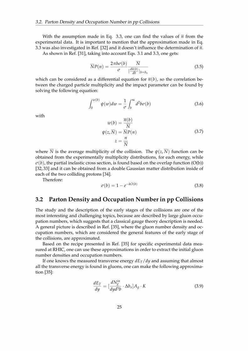
The study and the description of the early stages of the collisions are one of themost interesting and challenging topics, because are described by large gluon occu-pation numbers, which suggests that a classical gauge theory description is needed.A general picture is described in Ref. [35], where the gluon number density and oc-cupation numbers, which are considered the general features of the early stage ofthe collisions, are approximated.

Based on the recipe presented in Ref. [35] for specific experimental data mea-sured at RHIC, one can use these approximations in order to extract the initial gluonnumber densities and occupation numbers.

If one knows the measured transverse energy dET/dy and assuming that almostall the transverse energy is found in gluons, one can make the following approxima-tion [35]:

dET

dy= [

dNing

dyd3b· ∆bx]Ag · K (3.9)

25


where with b are denoted the coordinates of a point in the overlapping nuclei, ∆bz isthe longitudinal width of the volume occupied by gluons at their time of production,Ag is the area occupied by gluons and K is a gluon transverse momentum. Basedon this approximation, the gluon number densities averaged over the productionregion can be estimated, for an average value of K (for b⊥ = 0 - in the center of thenucleus, K ' Qs, where Qs is the gluon saturation momentum) [35].

More than that, the initial gluon number densities can give an estimation of thegluon occupation numbers, as follows:

f ing =

2π3

2 · (N2c − 1)

dNing

d3 pd3b' 2π3

2 · (N2c − 1)

dNing

dyd2b⊥d2 pT(3.10)

where the 2 denominator stands for the number of spin states available to gluonsand one can consider ∆y = ∆pz/pz ' ∆bz/pz; the following approximation also hasto be done:

dNing

dyd2bTd2 pT' 1

πQ2s

dNing

dyd2b⊥(3.11)

Following the recipe given in Ref. [35], the following estimates in terms of thegluon number densities of the initial state and of the gluon occupation number havebeen obtained:

TABLE 3.1: The estimations made on the gluon number densities of

the initial state (dNin

gdyd2b ) and of the gluon occupation number for the

most central collisions at the biggest RHIC energy and LHC energiesfor A-A and highest particle multiplicity for pp collisions at

√s = 7

TeV.

System Au-Au Pb-Pb pp√s(TeV) 0.2 2.76 5.02 7

dNing

dyd2b ( f m−1) ' 4.7 ' 11.8 ' 15.9 ' 18.7

f gin ' 0.9 ' 2.3 ' 3.1 ' 3.6

As one can observe in Table 3.1, a very interesting feature appears at the LHCenergies, where the initial gluon number density and occupation number seem tohave just a collision energy dependence, while the system size is playing a minorrole. This shows that similarities between A-A and pp collisions at LHC energies areexpected to be evidenced.

3.3 Review of the Main Results Obtained at LHC in SmallSystems and Similarities between pp, p-Pb and Pb-PbCollisions

The subject of small systems collision at LHC energies received an increased interestlately, since the studies of different observables at high multiplicity in pp collisions

26

3.3. Review of the Main Results Obtained at LHC in Small Systems and Similaritiesbetween pp, p-Pb and Pb-Pb Collisions

and in asymmetric (p-Pb) collision have revealed some collective-like effects, thatwere supposed to appear only in A-A collisions.

The CMS Collaboration found a very interesting feature when studying the two-particle correlations in pp at

√s = 7 TeV, discovering the long range near side ridge

structure in pp collisions at√

s = 7 TeV. For low pT values (pT ∈ [1-3] GeV/c) thenear side (∆φ ≈ 0) long range (2 ≤ |∆η| ≤ 4) correlation was observed [36] (Fig. 3.2(left)). Also, the pT spectra of identified hadrons were measured with high precisionat ALICE, where at low pT a hardening is observed in the pT spectra with increasingmultiplicity, feature that is very similar with the radial flow effect observed in heavyion collisions. More than that, in high multiplicity pp and p-Pb collisions, the pTspectra are very well described by the BGBW expression, inspired by hydrodynam-ical phenomenological models.

FIGURE 3.2: The comparison of the two particle correlation for highmultiplicity pp collisions at

√s = 7 TeV(left) [37] and Pb-Pb at

√sNN

= 2.76 TeV [38], on a finite range of ∆φ and ∆η.

The enhancement of strange and multi-strange hadron production in pp and p-Pb and its multiplicity dependence was also studied. In Fig. 3.3 can be observedan enhancement of strange to non-strange hadron production relative to pions inhigh multiplicity pp collisions, which is very similar to that obtained in p-Pb andperipheral Pb-Pb collisions. This enhancement could be a signature of the formationof QGP. However, core-corona relative contribution as a function of centrality couldexplain most of such a trend [13].

Another interesting effect observed in pp collisions is the depletion at low pTof proton to pion and proton to kaon ratio, which increases with multiplicity, butdecreases towards pT ≈ 1.4-2 GeV/c, feature than in A-A collisions was attributedto a collective transverse flow [39]. More than that, another similarity between pp,p-Pb and Pb-Pb colliding systems was observed in the BGBW fit parameters, thekinetic freeze-out temperature (T f o

kin) and the average radial flow velocity (< βT >)correlation (Fig. 3.4) [39]. In Fig. 3.4 the T f o

kin-< βT > correlation follows the sametrend and overlaps in pp at

√s = 7 TeV and in p-Pb at

√sNN = 5.02 TeV for the same

multiplicity classes, while the decrease of T f okin-< βT > with centrality is much more

enhanced in Pb-Pb collisions.

27

FIGURE 3.3: The yields of strange and multi-strange hadrons normal-ized to that of charged pions, as a function of particle multiplicity [?].

FIGURE 3.4: The comparison of BGBW fit parameters T f okin - < βT >

correlation for pp, p-Pb and Pb-Pb [39].

28

4 | Color Glass Condensate Scal-ing Variable

4.1 Expectations of < pT > Behavior as a Function of Colli-sion Energy and Centrality

As mentioned before, in the CGC model, where the bulk properties at small x de-grees of freedom are described by strong classical color fields, the gluon saturationis predicted at a corresponding saturation scale, Qs. The local parton-hadron dual-ity (LPHD) [40] picture is giving the dependence of the final multiplicities chargedhadrons on the initial gluon fields, based on the assumption that the final multiplic-ities are proportional to the initial partonic one and considered to be independent ofcollision energy or centrality because the conversion of partons into hadrons takesplace at a low virtuality scale, independent of the scale of the primary hard process.

If one assumes that in the LPHD framework, a gluon produces a number of ncharged particles in the collision, after fragmentation, so the initial gluons would bedescribed by [41, 42]:

< pT >g ∼ Qs

1S⊥

dNg

dη∼ Q2

s(4.1)

while for the final charged particles, due to the conservation of the transversemomentum during the fragmentation process, one gets:

< pT >ch ∼Qs

n1

S⊥dNch

dη∼ nQ2

s

(4.2)

which leads to:< pT >ch√

1S⊥

dNchdη

∼ 1n√

n(4.3)

In order to take into account the faster growth of multiplicity with the colli-sion energy in A-A than in pp, one needs to consider that the number of chargedhadrons produced in a gluon fragmentation is larger in A-A than in pp, whichimplies that the scaling values from Eq. 4.3 are smaller in central A-A collisions

29

Chapter 4. Color Glass Condensate Scaling Variable

than in pp, as is shown for RHIC data [14]. Since n increases with < pT >, the< pT > /

√(dN/dη)/S⊥ values should decrease with collision energy and cen-

trality, behaviour that is not very clear in [14]. Based on the latest result obtained atRHIC within the BES program at low energies and the latest results obtained at LHC,such a dependence is worth to be reconsidered. In the next sections, the recipe usedbased on experimental data in order to extract the CGC inspired scaling variable, ispresented.

4.2 dN/dy Estimates

Based on the correlation between the final state and the initial state from the LPHDpicture, we have considered the total hadron density per unit of rapidity for the scal-ing variable,

√(dN/dy)/S⊥. The data used for light flavour hadrons, pions kaons

and protons, were published in [14,43–45], while for hyperons the experimental datawere published in [46–52].

For the BES program, the experimental values of the yields were not reported for√sNN = 19.6 and 27 GeV in the case of hyperons, so the values were extracted by in-

terpolation, using energy dependence fits. Also, in the cases where some centralitieswere not reported, the corresponding values were obtained by interpolation usingthe centrality dependence fits. The yield values for Ω− and Ω+ were not reportedfor neither collision energy in the case of BES program, but from the extrapolationfrom the higher, available collision energies, to the BES ones, it has been shown thatthey have a negligible contribution, so the Ω− and Ω+ yields were neglected in thecase of BES.

In order to estimate the final values of the total hadron density over unit of ra-pidity, we have used the following expression, based on the previously mentionedpublished experimental data:

For BES energies:

dNdy' 3

2dNdy

(π++π−)

+ 2dNdy

(K++K−,p+ p,Ξ−+Ξ+)

+dNdy

(Λ+Λ)

(4.4)

For√

sNN = 62.4, 130 and 200 GeV:

dNdy' 3

2dNdy

(π++π−)

+ 2dNdy

(K++K−,p+ p,Ξ−+Ξ+)

+dNdy

(Λ+Λ,Ω−+Ω+)

(4.5)

For LHC energies:

dNdy' 3

2dNdy

(π++π−)

+ 2dNdy

(p+ p,Ξ−+Ξ+)

+dNdy

(K++K−,K0s+K0

s ,Λ+Λ,Ω−+Ω+)

(4.6)

For pp collisions at the LHC collision energy√

s = 7 TeV, the light flavour yieldswere estimated by integrating the pT spectra from Ref. [39], while for hyperons, theratio to pions given in Ref. [53] were extrapolated for higher multiplicites, so thefollowing approximation was used:

30

4.3. S⊥ Estimates for A-A Collisions

dNdy' 3

2dNdy

(π++π−)

+ 2dNdy

(p+ p,Ξ−+Ξ+,K0s )

+dNdy

(K++K−,Λ+Λ,Ω−+Ω+)

(4.7)

4.3 S⊥ Estimates for A-A Collisions

As already mentioned in a previous section, the theoretical tool that is used to de-scribe the geometry of a collision is the GMC framework. In this case, S⊥ whichrepresents the overlapping area between two colliding nuclei for a specific collisionenergy and centrality is estimated based on GMC approach. The nuclear densityprofile of the colliding nuclei is given in Eq. 2.1. Since w characterizes the deviationsfrom a spherical shape, it is considered w=0 for each nucleus, so Eq. 2.1 becomes:

ρ(r) =1

1 + exp( r−r0a )

(4.8)

with the corresponding input parameters for each nucleus: for the Au nucleus [14]:a = 0.535 fm,r0 = 6.5 fm and for the Pb nucleus [43] a = 0.546 fm, r0 = 6.62 fm.

Within the black disk approximation for nucleon-nucleon collisions, was usedEq. 2.3, for σNN

inel = σpp, with σpp as the nucleon-nucleon interaction cross section,for which the experimental data for the corresponding collision energies were takenfrom [14, 43, 54, 55]. All the information characterizing the collision were found inthe literature: for BES program [44] (Au-Au collisions, with

√sNN = 7.7, 11.5, 19.6,

27 and 39 GeV), for Au-Au at√

sNN = 62.4, 130 and 200 GeV [14] and for Pb-Pbcollisions at

√sNN = 2.76 TeV [43] and

√sNN = 5.02 TeV [45] at LHC.

FIGURE 4.1: An example of a GMC simulation of a Au-Au collisionat√

sNN = 200 GeV, at a given impact parameter (b = 6 fm), viewed inthe transverse plane; the nucleons of two colliding beams are repre-sented with different colors (red and blue), while for the participating

nucleons are used darker shades of red and blue [9].

31

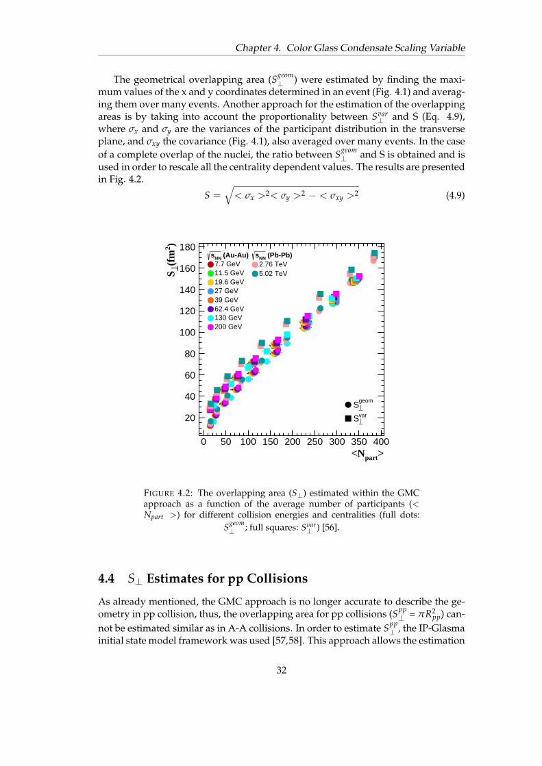
The geometrical overlapping area (Sgeom⊥ ) were estimated by finding the maxi-

mum values of the x and y coordinates determined in an event (Fig. 4.1) and averag-ing them over many events. Another approach for the estimation of the overlappingareas is by taking into account the proportionality between Svar

⊥ and S (Eq. 4.9),where σx and σy are the variances of the participant distribution in the transverseplane, and σxy the covariance (Fig. 4.1), also averaged over many events. In the caseof a complete overlap of the nuclei, the ratio between Sgeom

⊥ and S is obtained and isused in order to rescale all the centrality dependent values. The results are presentedin Fig. 4.2.

S =√< σx >2< σy >2 − < σxy >2 (4.9)

0 50 100 150 200 250 300 350 400>part<N

20

40

60

80

100

120

140

160

180)2 (

fmS

(Au-Au)NNs7.7 GeV11.5 GeV19.6 GeV27 GeV39 GeV62.4 GeV130 GeV200 GeV

(Pb-Pb)NNs2.76 TeV5.02 TeV

geomS

varS

FIGURE 4.2: The overlapping area (S⊥) estimated within the GMCapproach as a function of the average number of participants (<Npart >) for different collision energies and centralities (full dots:

Sgeom⊥ ; full squares: Svar

⊥ ) [56].

4.4 S⊥ Estimates for pp Collisions

As already mentioned, the GMC approach is no longer accurate to describe the ge-ometry in pp collision, thus, the overlapping area for pp collisions (Spp

⊥ = πR2pp) can-

not be estimated similar as in A-A collisions. In order to estimate Spp⊥ , the IP-Glasma

initial state model framework was used [57,58]. This approach allows the estimation

32

4.4. S⊥ Estimates for pp Collisions

of the maximal radius for which the energy density of the Yang-Mill fields is largerthan:

ε = αΛ4QCD (4.10)

The α values cannot be precisely estimated, but it’s limits are known: α ∈ [1, 10], andthe maximal radius for pp collisions is estimated in Ref. [57] for both α = 1 and α =10, as a function of the total number of gluons in the initial state, powered by (1/3)(Fig. 4.3).

FIGURE 4.3: The maximal radius esti-mated within the IP-Glasma initial statemodel, as a function of the total numberof gluons in the initial state to the power

of 1/3 [57].

FIGURE 4.4: The maximal radius depen-dence on the number of gluons to thepower of 1/3 taken from Ref. [57] for α= 1, fitted with the function given in Eq.

4.11 [58].

In Ref. [58], the rmax values were taken from Ref. [57] for α = 1 and fitted with thefollowing function (Fig. 4.4):

fpp =

0.387 + 0.0335x + 0.274x2 − 0.0542x3 if x < 3.4,1.538 if x ≥ 3.4.

(4.11)

In order to be consistent and take into account all the possible values that α can have,we have also analysed the α = 10 upper limit, so, based on the same recipe given inRef. [58], we have fitted the rmax values given in Ref. [57] for α = 10 (Fig. 4.3) withthe following expression:

fpp =

−0.018 + 0.3976x + 0.095x2 − 0.028x3 if x < 3.4,1.17 if x ≥ 3.4.

(4.12)

where x = (dNg/dy)1/3. The gluon density per unit of rapidity was approximatedby: dNg/dy ≈ dN/dy and the total hadron density per unit of rapidity was obtainedbased on Eq. 4.7.

The final values of the CGC inspired scaling variable,√(dN/dy)/Sgeom

⊥ as afunction of collision energies, for different centralities (A-A) and multiplicity classes(pp) are displayed in Fig. 4.5.

33


10 210 310 (GeV)NNs

1

1.5

2

2.5

3

3.5

4

4.5

)-1

(fm

geom

(dN

/ dy

) / S

(Au-Au & Pb-Pb)Centralities

0-5%

5-10%

10-20%

20-30%

30-40%

40-50%

50-60%

60-70%

70-80%

pp4Λ

4Λ 10

FIGURE 4.5: The scaling variable,√(dN/dy)/Sgeom

⊥ , as a function of√

sNN for different centralities and multiplicity classes. The dashedlines represent the fits performed using a power-law function for eachcentrality. In the case of pp collisions, the values are displayed forboth values of the α parameter (α = 1 dark red markers, α = 10 darkblue markers). For a better visualisation of these results, the dark blue

markers are artificially displaced in√

sNN [56].

34

5 | Results

As mentioned in the previous chapter, the assumptions made using the LPHD ap-proach and the correlation between the initial and final states, are giving the depen-

dence of < pT >/√(dN/dy)/Sgeom

⊥ from Eq. 4.3 as a function of the number of thecharged hadron produced in a gluon fragmentation. It is necessary to mention thatthe LPHD framework doesn’t take into account any collective effects, so the < pT >is expected to decrease with the increase of the collision energy and with central-ity. In this study, this dependence is studied for a wide range of energies (from 7.7GeV up to 5.44 TeV) and for different colliding systems (Au-Au, Cu-Cu, Pb-Pb andXe-Xe).

Based on the previous mentioned similarities between pp and A-A collisions, asystematic study between pp and Pb-Pb system at LHC energies of this scaling wasalso performed.

5.1 Systematic Study of the√

sNN Dependence

5.1.1 < pT > as a function of√( dN

dy )/Sgeom⊥

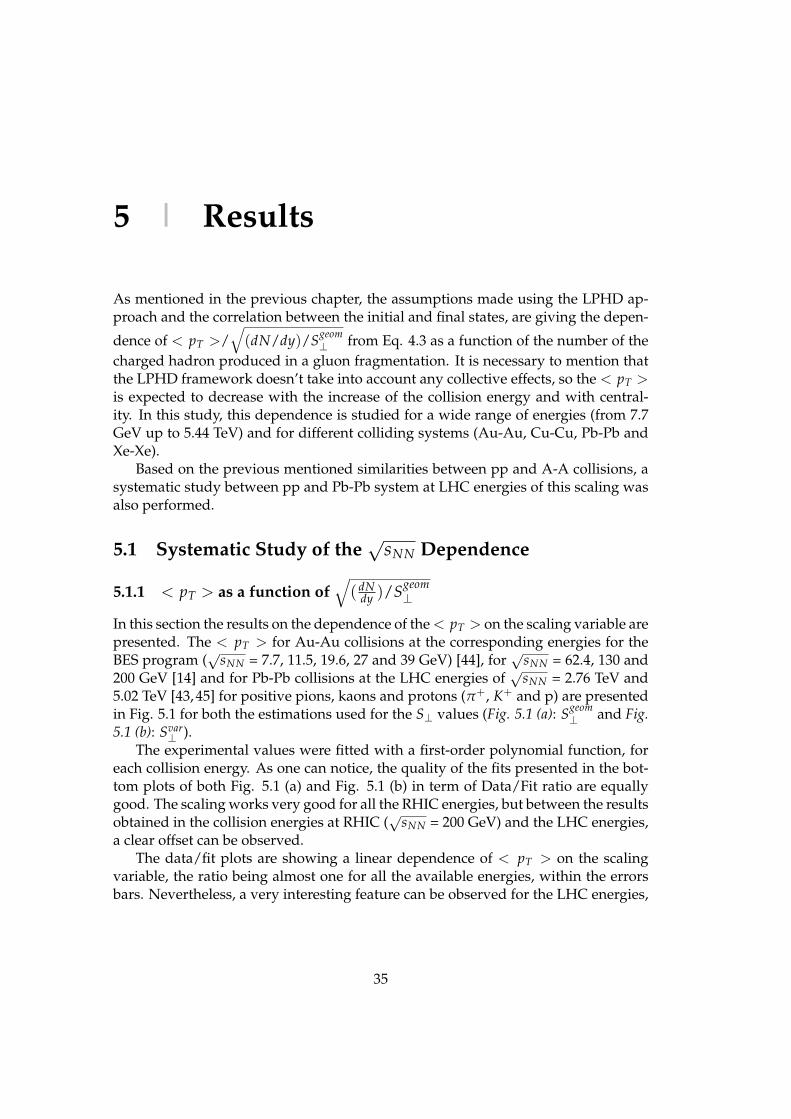
In this section the results on the dependence of the < pT > on the scaling variable arepresented. The < pT > for Au-Au collisions at the corresponding energies for theBES program (

√sNN = 7.7, 11.5, 19.6, 27 and 39 GeV) [44], for

√sNN = 62.4, 130 and

200 GeV [14] and for Pb-Pb collisions at the LHC energies of√

sNN = 2.76 TeV and5.02 TeV [43, 45] for positive pions, kaons and protons (π+, K+ and p) are presentedin Fig. 5.1 for both the estimations used for the S⊥ values (Fig. 5.1 (a): Sgeom

⊥ and Fig.5.1 (b): Svar

⊥ ).The experimental values were fitted with a first-order polynomial function, for

each collision energy. As one can notice, the quality of the fits presented in the bot-tom plots of both Fig. 5.1 (a) and Fig. 5.1 (b) in term of Data/Fit ratio are equallygood. The scaling works very good for all the RHIC energies, but between the resultsobtained in the collision energies at RHIC (

√sNN = 200 GeV) and the LHC energies,

a clear offset can be observed.The data/fit plots are showing a linear dependence of < pT > on the scaling

variable, the ratio being almost one for all the available energies, within the errorsbars. Nevertheless, a very interesting feature can be observed for the LHC energies,

35

Chapter 5. Results

0

0.2

0.4

0.6

0.8

1

1.2

1.4

1.6

> (G

eV/c

)T

 (G

eV/c

)T

 of positive pions, kaons and pro-

tons as a function of the scaling variable,√(dN/dy)/Sgeom

⊥ , for allthe measured energies and centralities in Au-Au at RHIC [14,44] andPb-Pb at LHC [43, 45]. The dashed lines represent the fits for each√

sNN with a first order polynomial function; Bottom: The ratio be-tween the experimental values and the values of a linear fit for eachcentrality and collision energy, in order to characterize the quality of

the fits. (b) The same as for (a), but for√(dN/dy)/Svar

⊥ [56].

where there is present a deviation from the general trend for the most central colli-sions, which can be interpreted as a sign of gluon saturation. However, this featurehas to be carefully further investigated.

The parameters of the linear fits from Fig. 5.1 are presented in Fig. 5.2, in terms ofthe slope (Fig. 5.2 (a)) and of the offset (Fig. 5.2 (b)). As one can notice, the slope val-ues are increasing form pions to protons. Even though the errors bars are rather large

for BES energies, a systematic decrease of the slope (< pT > /√(dN/dy)/Sgeom

⊥ ) isobserved (full symbols, continuous line), as theory predicts. This trend seems to bemass dependent, since it becomes more proeminent from pions to protons. In termsof Svar

⊥ (open symbols, dashed line), the slope is clearly smaller at lower collisionenergies. To better observe the dependence of the slope on the collision energy, thedata points were fitted with the following function:

f (x) = a +b

ln(x)(5.1)

In terms of the offsets (Fig. 5.2 (b)), their values are similar for all the RHIC en-ergies (from 7.7 GeV up to 200 GeV) and are systematically increasing for the LHCenergies (2.76 and 5.02 TeV) for all the three species, for both Sgeom

⊥ and Svar⊥ . The re-

sults obtained with the use of Svar⊥ are similar to those obtained from Sgeom

⊥ within theerror bars for pions and kaons, while for protons can be observed a systematicallygrowth of the offset values at RHIC energies. It is worth mentioning that for LHC

36

5.1. Systematic Study of the√

sNN Dependence

10 210 310 (GeV)NNs

0

0.05

0.1

0.15

0.2

0.25

0.3

0.35

0.4

Slop

e

+π+K

p

geomS

varSa)

0

0.2

0.4

0.6 b)

0

0.2

0.4

0.6

Off

set

10 210 310 (GeV)NNs

0

0.2

0.4

0.6

FIGURE 5.2: (a) The slope of the < pT >= f (√(dN/dy)/S⊥) (Fig.

5.1) for√(dN/dy)/Sgeom

⊥ ) (full symbols) and for√(dN/dy)/Svar

⊥ )

(open symbols). The slope dependence on the collision energy,√

sNNis fitted with the function given in Eq. 5.1 (Sgeom

⊥ - continuous line;Svar⊥ - dashed line), separately for pions (blue markers), kaons (green

markers) and protons (red markers); (b) The offsets of the < pT >=

f (√(dN/dy)/S⊥) (Fig. 5.1) as a function of collision energy, sepa-

rately for pions (top), kaons (center) and protons (bottom) [56].

energies, the values of both the slopes and offsets are the same when using Sgeom⊥ and

Svar⊥ . Since the observed trends are rather similar in both cases of S⊥ = Sgeom

⊥ and S⊥= Svar⊥ , the results will be presented only in terms of Sgeom

⊥ .

Core-Corona Interplay

In order to see in which extent the saturation trend observed in the most central col-lisions at the LHC energies are due to the core-corona interplay and how does the< pT >= f (

√(dN/dy)/S⊥) dependence look like for the core contribution, a fur-

ther investigation in terms of core-corona interplay was performed. For√

sNN = 200GeV (Au-Au collisions) and for

√sNN = 2.76 and 5.02 TeV (Pb-Pb collisions) we es-

timated the core contributions in terms of mean transverse momentum (< pT >core)

and scaling variable (√(dN/dy)core/(Sgeom

⊥ )core) based on the recipe given in Ref.[13] and previously described in Section 2.3. The < pT >corona and (dN/dy)corona

values were measured in ppMB collisions, reported in Ref. [14] for√

sNN = 200 GeV,by the STAR Collaboration, while for

√sNN = 2.76 and 5.02 TeV the experimental

values for minimum bias pp collisions were reported in Refs. [59, 60] by the ALICECollaboration.

A comparison between the experimental values and the corresponding values ofthe extracted core contribution is presented in Fig. 5.3. In order to extract some quan-titative information about the different trends of all experimental vs. core < pT >

37

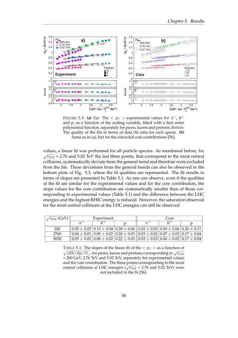
Chapter 5. Results

0

0.2

0.4

0.6

0.8

1

1.2

1.4

1.6

> (G

eV/c

)T

<pNNs

200 GeV2.76 TeV5.02 TeV

Experiment

Particles+π+K

p

a)

2 2.5 3 3.5 4 4.50.81

1.2 +π

2 2.5 3 3.5 4 4.50.81

1.2

Dat

a/F

it +K

2 2.5 3 3.5 4 4.5


0.81

1.2 p

0

0.2

0.4

0.6

0.8

1

1.2

1.4

1.6

> (G

eV/c

)T

<p

NNs200 GeV2.76 TeV5.02 TeV

Core

Particles+π+K

p

b)

2 2.5 3 3.5 4 4.5Data / Fit

0.81

1.2 +π

2 2.5 3 3.5 4 4.50.81

1.2

Dat

a/F

it +K

2 2.5 3 3.5 4 4.5


0.81

1.2 p

FIGURE 5.3: (a) Top: The < pT > experimental values for π+, K+

and p, as a function of the scaling variable, fitted with a first orderpolynomial function, separately for pions, kaons and protons; Bottom:The quality of the fits in terms of data/fit ratio for each specie. (b)

Same as in (a), but for the extracted core contributions [56].

values, a linear fit was performed for all particle species. As mentioned before, for√sNN = 2.76 and 5.02 TeV the last three points, that correspond to the most central

collisions, systematically deviate from the general trend and therefore were excludedfrom the fits. These deviations from the general trends can also be observed in thebottom plots of Fig. 5.3, where the fit qualities are represented. The fit results interms of slopes are presented In Table 5.1. As one can observe, even if the qualitiesof the fit are similar for the experimental values and for the core contribution, theslope values for the core contribution are systematically smaller than of those cor-responding to experimental values (Table 5.1) and the difference between the LHCenergies and the highest RHIC energy is reduced. However, the saturation observedfor the most central collisions at the LHC energies can still be observed.

√sNN (GeV) Experiment Core

π+ K+ p π+ K+ p200 0.05 ± 0.02 0.13 ± 0.04 0.28 ± 0.06 0.02 ± 0.03 0.09 ± 0.06 0.20 ± 0.112760 0.04 ± 0.01 0.09 ± 0.02 0.20 ± 0.03 0.03 ± 0.02 0.07 ± 0.03 0.17 ± 0.045020 0.05 ± 0.02 0.08 ± 0.02 0.22 ± 0.03 0.03 ± 0.03 0.06 ± 0.02 0.17 ± 0.04

TABLE 5.1: The slopes of the linear fit of the < pT > as a function of√(dN/dy)/S⊥, for pions, kaons and protons corresponding to

√sNN

= 200 GeV, 2.76 TeV and 5.02 TeV, separately for experimental valuesand the core contribution. The three points corresponding to the mostcentral collisions at LHC energies (

√sNN = 2.76 and 5.02 TeV) were

not included in the fit [56].

38

sNN Dependence

5.1.2 < pT > mass dependence as a function of√( dN

dy )/Sgeom⊥

The slope of the < pT > dependence on particles mass (pions, kaons and protons)can give an insight on the dynamics of the collision, if one takes into account thebasic definition of the momentum of a particle with mass. The < pT > = f(mass)dependences are linear for each centrality, except for the most peripheral ones, sofits with linear functions were performed for these dependences, for all collisionenergies and centralities. The parameters of this fits are represented in Fig. 5.4 ((a)-particles; (b)-antiparticles) in terms of the slopes of these fits, while in Fig. 5.5 ((a)-particles; (b)-antiparticles) are represented the corresponding offsets.

)-1 (fmgeom

(dN / dy) / S

0

0.2

0.4

0.6

0.8

1

1.2

1.4

1.6

> =

f(m

ass)

TSl

ope:

<p

Au-Au7.7 GeV11.5 GeV19.6 GeV27 GeV39 GeV62.4 GeV130 GeV200 GeV

Pb-Pb2.76 TeV5.02 TeV

Particles, p+, K+π

0.04± = -0.33 α 0.04± = 1.57 β 0.04± = 0.64 γ

a)

1 1.5 2 2.5 3 3.5 4 4.5


0.60.8

11.21.4

Dat

a / F

it

)-1 (fmgeom

(dN / dy) / S

0

0.2

0.4

0.6

0.8

1

1.2

1.4

1.6

> =

f(m

ass)

TSl

ope:

= f (mass) dependencefor π+, K+ and p, as a function of the scaling variable, fitted with theexpression given in Eq. 5.2, with the parameters listed in the figure;Bottom: The quality of the fits in terms of data/fit ratio. (b) Same as

in (a), but for the associated antiparticles (π−, K− and p) [56].

The slope dependencies on the scaling variable from Fig. 5.4 are fitted with theexpression given in Eq. 5.2 and the fit parameters are also displayed in Fig. 5.4. Asone can observe, in terms of the slope of < pT >= f (mass) dependence (Fig. 5.4) avery good scaling was obtained for both particles (Fig. 5.4 (a)) and antiparticles (Fig.5.4 (b)), that follows the trend of Eq. 5.2 very closely, within the error bars, exceptfor√

sNN = 19.6, 27 and 39 GeV, for which the slopes are slightly deviating from thegeneral trends. The quality of the fits is presented in the bottom plots, in terms ofdata/fit ratio.

Slope<pT>= f (mass) = α + β(√(dN/dy)/Sgeom

⊥ )γ (5.2)

The corresponding offsets of the < pT >= f (mass) dependence are representedin Fig. 5.5, separately for particles (Fig. 5.5 (a)) and antiparticles (Fig. 5.5 (b)). Evenif the error bars are rather large, for the LHC energies there can be observed almost

39

Chapter 5. Results

1 1.5 2 2.5 3 3.5 4 4.5


0.26

0.28

0.3

0.32

0.34

0.36

0.38

0.4

0.42

0.44

0.46

> =

f(m

ass)

TO

ffse

t: =

f(m

ass)

TO

ffse

t: = f (mass) dependence forπ+, K+ and p, as a function of the scaling variable; (b) Same as in (a),

but for the associated antiparticles (π−, K− and p) [56].

a constant value, while for collision energies up to 62.4 GeV, a systematic increase is

observed for√(dN/dy)/Sgeom

⊥ < 1.7 f m−1.

10 210 310 (GeV)NNs

0.2

0.25

0.3

0.35

0.4

0.45

0.5

> =

f(m

ass)

T<O

ffse

t>:

= f (mass) offsets, cor-

responding to√(dN/dy)/Sgeom

⊥ ≥ 1.7 f m−1 as a function of collisionenergy,

√sNN , for particles (π+, K+, p - full symbols) and antiparti-

cles (π−, K−, p - open symbols) [56].

40

sNN Dependence

For values of√(dN/dy)/Sgeom

⊥ larger than 1.7 f m−1 a plateau is reached for allthe collision energies. In order to observe a

√sNN dependence, we have averaged for

each collision energy only the offset values corresponding to√(dN/dy)/Sgeom

⊥ ≥1.7 f m−1. The results obtained are represented in Fig. 5.6, for both particles (fullsymbols) and antiparticles (open symbols).

5.1.3√( dN

dy )/Sgeom⊥ dependence of Boltzmann-Gibbs Blast Wave Fit pa-

rameters

The Boltzmann Gibbs blast wave (BGBW) expression (Eq. 5.3), inspired from hydro-dynamical models [28] which make phenomenological assumptions that the parti-cles produced in a system are locally thermalized at a kinetic freeze-out temperatureand they develop a collective behavior, moving with a collective transverse flow ve-locity, that is common for all the particles involved. At this stage of the collision, theparticles can be considered as a fireball, that is modelled under the assumption thatit has an azimuthally isotropic shape, characterized by a kinetic freeze-out tempera-ture (T f o

kin) and a transverse flow velocity (βT). The BGBW expression (Eq. 5.3) givesa very good description of particles spectra, by taking into account these collectiveeffects.

dNpTdpT

∝∫ R

0rdrmT I0(

pTsinh(ρ)

T f okin

)K1(mTcosh(ρ)

T f okin

) (5.3)

withρ = tanh−1(βT)

mT =√

p2T + m2

0

βT(r) = βs(rR)n

(5.4)

where I0 and K1 represent the modified Bessel functions, βs is the surface velocity,(r/R) is the relative radial position in the fireball and n defines the expansion profile.

In order to extract the freeze-out properties of the collision from the availabledata, the pT spectra of π+, K+ and p and those of their corresponding antiparticles(π−, K−, p) were fitted simultaneously with the BGBW expression (Eq. 5.3), withthree free parameters: βs, T f o

kin and n. The mean values of the transverse flow velocity,< βT >, were found using the expression given in Eq. 5.5. All the available data for< βT > [14, 43–45, 61] as a function of the scaling variable, are presented in Fig. 5.7.

< βT >=2

2 + nβs (5.5)

Another aspects that one has to consider are the differences between particlesand antiparticles pT spectra, that become more prominent with the decrease of thecollision energy,

√sNN . In order to see in which extent the particles and antiparticles

behave differently, for some energies and centralities where azimuthal dependentBGBW fits were performed [62, 63], the < βT > values for antiparticles were plot-ted in Fig. 5.7 (open symbols), while the full symbols represent the case when pT

41

Chapter 5. Results

)-1 (fmgeom

(dN / dy) / S

0

0.1

0.2

0.3

0.4

0.5

0.6

0.7

0.8

0.9>Tβ<



All particlesAntiparticles

4x4 + a3x3 + a2x2x + a1 + a0Fit function: a 0.04± = -1.16 0a

0.04± = 1.78 1a 0.01± = -0.72 2a

0.00± = 0.14 3a 0.00± = -0.01 4a

1 1.5 2 2.5 3 3.5 4 4.5

)-1 (fmgeom

(dN / dy) / S

0

0.5

1

1.5

2

Dat

a / F

it

FIGURE 5.7: Top: The BGBW fit parameter < βT > values as a

function of the scaling variable,√(dN/dy)/Sgeom

⊥ , taking into accountonly the antiparticles (open symbols) and all the particles (full sym-bols) - fitted with a 4th order polynomial function; Bottom: The quality

of the fit as data/fit ratio [56].

spectra of all particles (both particles and antiparticles) are fitted with the BGBWexpression simultaneously. One can observe in Fig. 5.7 that the differences betweenthese two cases are less and less significant with increasing the collision energy, be-ing very prominent for

√sNN = 11.5 GeV and almost negligible for

√sNN = 62.4

GeV, so it becomes very important that one takes into account separately the contri-butions of particles and antiparticles, since at low energies there are more particlesproduced in the collision than antiparticles, the contribution in the observed trendsbeing almost entirely dominated by particles. In Fig. 5.7, one can observe that for thepublished < βT > values, a very good scaling as a function of the scaling variable

(√(dN/dy)/Sgeom

⊥ ) was obtained, described rather good by a 4th order polynomialfunction that was used as a fit function for all energies and centralities (the parame-ters of the fit function are displayed in Fig. 5.7). In the bottom plot, the fit quality isdisplayed as data/fit ratio, where one can observe that for all the collision energiesthe data scale rather good, except for the most peripheral collisions correspondingto the lowest BES available energies (

√sNN = 7.7 and 11.5 GeV).

The dynamics of the < βT > BGBW parameter can be observed in Fig. 5.8 where

42

sNN Dependence

1 1.5 2 2.5 3 3.5 4 4.5

)-1 (fm geom (dN / dy) / S

0.5

1

1.5

2

2.5

3

3.5

4

4.5

5>P

erip

hera

l

Tβ>

/ <Tβ

Rat

io:

<



FIGURE 5.8: The ratio between the < βT > values and the ones cor-responding the the most peripheral collisions, as a function of the

scaling variable,√(dN/dy)/Sgeom

⊥ [56].

values of < βT > corresponding to each centrality were divided to the most periph-eral (58-85% for

√sNN = 130 GeV and 70-80% for all the other collision energies)

< βT > values, at the corresponding collision energy. The values oh the < βT >

/ < βT >Peripheral ratio are plotted in Fig. 5.8 as a function of√(dN/dy)/Sgeom

⊥ .

In Fig. 5.9, the data for the kinetic freeze-out temperature (T f okin) and for the

expansion profile parameter, n [14, 43–45, 61] as a function of the scaling variable,√(dN/dy)/Sgeom

⊥ , are presented. Due to rather large errors bars, one could con-clude only on a global trend, i.e. for the RHIC values (

√sNN = 7.7 up to 200 GeV)

the T f okin show an almost linear decrease, while a shift of almost 20 MeV is observed

when moving from the highest energy available at RHIC to LHC energies, as for the< pT > dependence (Fig. 5.1) or for the offset of < pT > = f (mass) dependence(Fig. 5.5). From Fig. 5.9 (b), is not evidenced only systematic energy dependence ofthe n BGBW fit parameter, the parameter’s values being scattered, with an oppositetrend for

√sNN = 62.4 and 200 GeV than for the LHC energies. It is very important

to have in mind that different fit ranges were used in the literature [14, 43–45,61] forthe BGBW fit expression, so the consistency of this study may be affected. The dif-ferent pT ranges used for the fit expression are selected in order to reduce as muchas possible the contributions of other processes, like resonance decays in the case of

43

Chapter 5. Results

low pT pions, or suppression effects for higher pT values for all particle species.

1 1.5 2 2.5 3 3.5 4 4.5

)-1 (fm geom (dN / dy) / S

0.08

0.1

0.12

0.14

0.16 (G

eV)

fo kin

T



a)

1 1.5 2 2.5 3 3.5 4 4.5


0

0.2

0.4

0.6

0.8

1

1.2

1.4

1.6n Au-Au7.7 GeV11.5 GeV19.6 GeV27 GeV39 GeV62.4 GeV130 GeV200 GeV

Pb-Pb2.76 TeV5.02 TeVb)

FIGURE 5.9: (a) The T f okin BGBW fit parameter as a function of the

geometric variable,√(dN/dy)/Sgeom

⊥ ; (b) Same as in (a), but for then parameter [56].

0.1 0.2 0.3 0.4 0.5 0.6 0.7

>T

β<

0.06

0.08

0.1

0.12

0.14

0.16

0.18

(G

eV)

fo kin

T



FIGURE 5.10: The T f okin BGBW fit parameter dependence on < βT >

[56].

44

5.2. Systematic Study of the System Size Dependence

In Fig. 5.10 the kinetic freeze-out temperature BGBW fit parameter is plotted asa function of the average transverse flow velocity ( T f o

kin = f(< βT >)). A systematicscaling is observed for all the RHIC energies, while the same shift can be observedbetween the highest RHIC energy and the LHC energies.

5.2 Systematic Study of the System Size Dependence

5.2.1 Heavy Ion Collisions

In order to take into account the role played by the system size in this CGC inspiredscaling, we have compared several colliding systems for the same or with a slightlydifferent collision energy. In this study we have compared the Cu-Cu and Au-Aucollision systems, both measured at

√sNN = 200 GeV at RHIC, but we have also

extended this study to heavier systems at a much higher collision energy, like Pb-Pb and Xe-Xe, at

√sNN = 5.02 TeV and 5.44 TeV, respectively. The scaling variable

for these new systems was estimated as described in Chapter 4, with data for Xe-Xeavailable in Refs. [64, 65] and for Cu-Cu available in Refs. [66, 67].

2 2.5 3 3.5 4 4.5


0

0.2

0.4

0.6

0.8

1

1.2

1.4

1.6

> (G

eV/c

)T

 dependence on the scaling variable,√(dN/dy)/Sgeom

⊥ , for positive pions (blue markers), kaons (greenmarkers) and protons (red markers), for different colliding systems

and energies [68].

45

Chapter 5. Results

0

0.2

0.4

0.6

0.8

1

1.2

1.4

1.6

> =

f(m

ass)

TSl

ope:

 =f(mass) as a function of the scaling variable,√(dN/dy)/Sgeom

⊥ , fitted with the expres-sion given in Eq. 5.2, for different collidingsystems and energies; Bottom: The quality

of the fit in terms of data/fit ratio [68].

0

0.1

0.2

0.3

0.4

0.5

0.6

0.7

0.8>Tβ<


3x3 + + a2x2x + a1 + a0Fit function: a

0.07± = -0.43 0a 0.06± = 0.70 1a 0.02± = -0.16 2a 0.00± = -0.02 3a

1.5 2 2.5 3 3.5 4 4.5


0.60.8

11.21.4

Dat

a / F

it

FIGURE 5.13: Top: The average valuesof the BGBW fit parameter, < βT >,as a function of the scaling variable,√(dN/dy)/Sgeom

⊥ , fitted with a 3rd orderpolynomial function, for different collidingsystems and energies; Bottom: The quality

of the fit in terms of data/fit ratio [68].

In Fig. 5.11, one can observe a very good scaling between the LHC energies,for similar collision energies: Pb-Pb at

√sNN = 5.02 TeV and Xe-Xe at

√sNN = 5.44

TeV. When moving to much lower collision energies at RHIC (√

sNN = 200 GeV) anddifferent symmetric systems (Au-Au and Cu-Cu), a shift to larger values is observedfor Cu-Cu, relative to Au-Au, the shift decreasing from pions to protons. Whencomparing all these collision systems at different energies, one can notice a shiftbetween RHIC and LHC energies.

In terms of the slope of the < pT > as a function of mass of pions, kaons andprotons (Fig. 5.12) and for the average values of the BGBW fit parameter, < βT >

(Fig. 5.13) as a function of scaling variable,√(dN/dy)/Sgeom

⊥ , one can observe a verygood scaling for all the different symmetric systems (Cu-Cu: blue markers; Au-Au:magenta markers; Xe-Xe: red markers and Pb-Pb: green markers) and energies. Theslopes of < pT > = f(mass) dependences on the scaling variable were fitted withthe expression given in Eq. 5.2, with the parameters displayed in Fig. 5.12, while

the BGBW fit parameter’s dependence on√(dN/dy)/Sgeom

⊥ was fitted with a third-order polynomial function, with parameters displayed in Fig. 5.13. The qualities ofthe fits are displayed in the bottom plots of each figure.

5.2.2 Small systems (pp) versus heavy systems (Pb-Pb) at LHC energies

As previously mentioned, since several similarities were observed between pp andPb-Pb systems, the small systems have started to play a major interest by themselves,and not only as heavy-ion collisions references. The results presented in this section

46

5.2. Systematic Study of the System Size Dependence

1.5 2 2.5 3 3.5 4 4.5)-1 (fmgeom(dN / dy) / S

0

0.2

0.4

0.6

0.8

1

1.2

1.4

1.6

> (G

eV/c

)T

 as a function of scaling variable, for posi-tive pions, kaons and protons, for Pb-Pb (

√sNN = 2.76 TeV (squares)

and 5.02 TeV (triangles)) and pp (α = 1: dark red markers; α = 10: darkblue markers) [56].

were obtained in order to see how this scaling can reveal similarities between pp(√

s = 7 TeV) and Pb-Pb (√

sNN = 2.76 and 5.02 TeV) colliding systems, in terms ofthe already mentioned observables (< pT >, the slope of < pT > = f(mass) and< βT >). The recipes used in order to obtain the scaling variable is presented inChapter 4, for both pp and Pb-Pb systems. In order to be consistent, in the pp case,since the overlapping area has two limits, for α = 1 and for α = 10, and the values ofα can’t be precisely known (α ∈ [1, 10]), the scaling variable was estimated for bothvalues, the results in between (α = 1: dark red markers; α = 10: dark blue markers)being represented by a shaded area.

In the pp case, the < pT > values were obtained by fitting the published pTspectra [39] with the following expression [69]:

dσ

pTdpT= Aeexp(

−EkinT

Te) +

A

(1 + p2T

T2n )n

(5.6)

which was found to best describe the experimental data.In Fig. 5.14 the comparison between pp and Pb-Pb at LHC energies is presented,

in terms of the dependence of the < pT > on the scaling variable. As one can ob-serve, a general trend seems to set in for both pp and Pb-Pb systems, for all the three

47

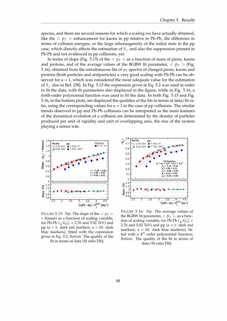
Chapter 5. Results

species, and there are several reasons for which a scaling we have actually obtained,like the < pT > enhancement for kaons in pp relative to Pb-Pb, the difference interms of collision energies, or the large inhomogeneity of the initial state in the ppcase, which directly affects the estimation of S⊥ and also the suppression present inPb-Pb and not evidenced in pp collisions, yet.

In terms of slope (Fig. 5.15) of the < pT > as a function of mass of pions, kaonsand protons, and of the average values of the BGBW fit parameter, < βT > (Fig.5.16), obtained from the simultaneous fits of pT spectra of charged pions, kaons andprotons (both particles and antiparticles) a very good scaling with Pb-Pb can be ob-served for α = 1, which was considered the most adequate value for the estimationof S⊥ also in Ref. [58]. In Fig. 5.15 the expression given in Eq. 5.2 was used in orderto fit the data, with fit parameters also displayed in the figure, while in Fig. 5.16, aforth-order polynomial function was used to fit the data. In both Fig. 5.15 and Fig.5.16, in the bottom plots, are displayed the qualities of the fits in terms of data/fit ra-tio, using the corresponding values for α = 1 in the case of pp collisions. The similartrends observed in pp and Pb-Pb collisions can be interpreted as the main featuresof the dynamical evolution of a collision are determined by the density of particlesproduced per unit of rapidity and unit of overlapping area, the size of the systemplaying a minor role.

)-1 (fmgeom

(dN / dy) / S

0

0.2

0.4

0.6

0.8

1

1.2

1.4

1.6

> =

f(m

ass)

TSl

ope:

= f(mass) as a function of scaling variable,for Pb-Pb (

√sNN = 2.76 and 5.02 TeV) and

pp (α = 1: dark red markers; α = 10: darkblue markers), fitted with the expressiongiven in Eq. 5.2; Bottom: The quality of the

fit in terms of data/fit ratio [56].

)-1 (fmgeom

(dN / dy) / S

0

0.1

0.2

0.3

0.4

0.5

0.6

0.7

0.8>Tβ<


pp4Λ7 TeV:

4Λ7 TeV: 10

Fit function4x4 + a3x3 + a2x2x + a1 + a0a

0.12± = -1.11 0a 0.11± = 1.66 1a 0.03± = -0.68 2a

0.01± = 0.14 3a 0.00± = -0.01 4a

1.5 2 2.5 3 3.5 4 4.5)-1 (fm

geom(dN / dy) / S

0.60.8

11.21.4

Dat

a / F

it

FIGURE 5.16: Top: The average values ofthe BGBW fit parameter, < βT >, as a func-tion of scaling variable, for Pb-Pb (

√sNN =

2.76 and 5.02 TeV) and pp (α = 1: dark redmarkers; α = 10: dark blue markers), fit-ted with a 4th order polynomial function;Bottom: The quality of the fit in terms of

data/fit ratio [56].

48

6 | Summary and Outlook

In this thesis, based on the published data at RHIC and LHC, a systematic study wasperformed in terms of the dependence of different observables on the geometricalvariable inspired from the CGC model, for a wide range of energies (

√sNN from 7.7

GeV up to 5.44 TeV), for several colliding systems (Cu-Cu, Au-Au, Pb-Pb, Xe-Xe andpp) and centralities for A-A, or multiplicity classes for pp collisions.

The available experimental < pT > values follow a rather good scaling forthese energies, with a jump from the highest available energy measured at RHIC

to those at LHC. After fitting each < pT > = f(√(dN/dy)/Sgeom

⊥ ) with a straightline, the obtained slopes are showing a collision energy and mass dependent be-havior: the slopes are increasing from pions to protons, while decreasing towardshigher values of the collision energy (from BES to LHC). There was also evidenceda possible sign of gluon saturation for the most central collisions corresponding toLHC energies. The behavior of the experimental < pT > values as a function ofthe scaling variable supports the theoretical predictions from Ref. [42], where the< pT > /

√(dN/dy)/S⊥ values were expected to decrease as a function of collision

energy and centrality. A study of the core-corona effects for√

sNN = 200 GeV, 2.76TeV and 5.02 TeV was made. The results obtained for the core contribution in termsof < pT > and scaling variable and a comparison between these results and the ex-perimental ones was also presented in this study. It was shown that if one takes intoaccount only the core contribution, a better scaling was obtained, since the differencebetween the highest energy measured at RHIC and the LHC energies in terms of the< pT > slope as a function of

√(dN/dy)/S⊥ is reduced for the core contribution.

Moreover, the < pT > /√(dN/dy)/S⊥ trend is also considerably attenuated. The

saturation trend observed at the LHC energies for the most central collision is stillobserved for the core contribution.

In terms of the slope of the < pT > as a function of mass of pions, kaons andprotons, its dependence on the scaling variable has shown a much better scaling,and also for the BGBW fit parameter, the average transverse flow velocity, < βT >.The T f o

kin and the offset of the < pT > = f(√(dN/dy)/S⊥) dependence are showing a

jump between RHIC and LHC energies, possibly due to the interplay of other effectslike suppression and its azimuthal dependence, or the hydrodynamic expansion inthe final stages after hadronization that have to be carefully considered.

These similarities were also present in the pp and Pb-Pb comparison. A nicerepresentation was obtained in terms of the < pT > dependence, where the ppand Pb-Pb systems have shown similar trends, while for the slope of the < pT > =

49

Chapter 6. Summary and Outlook

f(mass) and for the BGBW fit parameter, < βT >, actual scalings were obtained, forthe case of α = 1.

This study supports the conclusion that the global features extracted from heavyion collisions from the lowest RHIC energy, up to the highest LHC collision energyare dependent on the number of hadrons produced over unit of rapidity and unit ofoverlapping area, while the system size is playing a minor role.

In the near future we would like to extend this study to some unexploited, yetinteresting observables. Based on the different behavior of heavier hadrons afterthe hadronization stage, the dependence on the geometrical variable of the differentobservables describing the hyperons should be carefully studied. Furthermore, newexperimental data for pp collisions at a higher collision energy, i.e. 13 TeV, that willimprove statistics in high multiplicity events, are now available. Moreover, in allthese further studies, the core-corona contribution should be carefully taken intoaccount.

50

Bibliography

[1] S. Schramm W. Greiner and E. Stein. Quantum Chromodynamics. 2007.

[2] S. Bethke. J.Phys.G26:R27, 2000.

[3] K. Fukushima and T. Hatsuda. Rept.Prog.Phys.74:014001, 2011.

[4] K. Rajagopal. Nucl.Phys.A 661, 1999.

[5] R. Placakyte (on behalf of the H1 and ZEUS Collaborations). Proceedings, 31stInternational Conference on Physics in collisions (PIC 2011): Vancouver, Canada, Au-gust 28-September 1, 2011.

[6] H1 Collaboration. Nucl.Phys.B 470 (1996), Eur.Phys.J.C 7:609 (1999).

[7] J. Jalilian-Marian F. Gelis, E. Iancu and R. Venugopalan. Ann.Rev.Nucl.Part.Sci.60, 2010.

[8] T. Lappi and L. McLerran. Nucl.Phys.A 772:200-212, 2006.

[9] S.J. Sanders M.L. Miller, K. Reygers and P. Steinberg.Ann.Rev.Nucl.Part.Sci.57:205-243, 2007.

[10] K. Werner. Phys.Rev.Lett. 98:152301, 2007.

[11] K. Werner J. Aichelin. Phys.Rev.C 79:064907, 2009.

[12] K. Werner J. Aichelin. Phys.Rev.C 82:034906, 2010.

[13] M. Petrovici et al. Phys.Rev.C 96:014908, 2017.

[14] B.I. Abelev et al. (STAR Collaboration). Phys.Rev.C 79:034909, 2009.

[15] M. Sumbera (STAR Collaboration). Acta Phys.Polon.Supp.6:429-436, 2013.

[16] M. Petrovici et al. AIP Conf.Proc. 1852:050003, 2017.

[17] S. Horvat. PhD Thesis: Measurement of the collision energy dependence of jet-quenching signatures of de-confinement at STAR, 2017.

[18] S. Horvat (STAR Collaboration). 8th International Workshop on Critical Point andOnset of Deconfinement, March 11-15, Napa, California, USA, 2013.

[19] J. Adams et al. (STAR Collaboration). Phys.Rev.Lett. 91:172302, 2003.

51

BIBLIOGRAPHY

[20] ATLAS Collaboration. JHEP 09:050, 2015.

[21] ATLAS Collaboration. ATLAS-CONF-2017-012, 2017.

[22] B. Abelev et al. (ALICE Collaboration). Phys.Rev.C 88:044910, 2013.

[23] ALICE Collaboration. Phys.Rev.Lett. 116:222302, 2016.

[24] L. Kumar (STAR Collaboration). Nucl.Phys.A, 904-905:256c-263c, 2013.

[25] I. Adam et al. (ALICE Collaboration). Phys.Rev.C 94:034903, 2016.

[26] K. Aamodt et al. (ALICE Collaboration). Phys.Rev.Lett. 105:252301, 2010.


[28] E. Schnedermann U. Heinz and J. Sollfrank. Phys.Rev.C 48:2462, 1993.

[29] ALICE Collaboration. Phys.Lett.B 696:328, 2011.

[30] B. Abelev et al. (ALICE Collaboration). Phys.Lett.B 736:196-207, 2014.

[31] H. Moreno. Phys.Rev.D8, 1973.

[32] A. Bialas and E. Bialas. Acta.Phys.Polonica B5, 1974.

[33] I. Dawson C. Buttar and A. Moraes. Eur.Phys.J. C50, 2007.

[34] ATLAS Collaboration. ATL-PHYS-PUB-2010: 002, 2010.

[35] A.H. Mueller. Nucl.Phys.A 715:20c-34c, 2003.

[36] V. Khachatryan et al. (CMS Collaboration). J.High Energy Phys. 09:091, 2010.

[37] D. Velicanu (CMS Collaboration). J.Phys.G: Nucl.Part.Phys. 38:124051, 2011.


[39] C. Andrei (ALICE Collaboration). Nucl.Phys.A 931:c888, 2014.

[40] V.A. Khoze Y.L. Dokshitzer and S. Troian. J.Phys.G 17:1585, 1991.

[41] T. Lappi. Eur.Phys.J C71:1699, 2011.

[42] E. Levin and A.J. Rezaeian. Phys.Rev.D 83:114001, 2011.


[44] L. Adamczyk et al. (STAR Collaboration). Phys.Rev.C 96:044904, 2017.

[45] N. Jacazio (ALICE Collaboration). Nucl.Phys.A 967:421, 2017.

[46] X. Zhu (STAR Collaboration). in Critical Point and Onset of Deconfinement(CPOD), 7-11.11.2011, Wuhan, China (unpublished), 2011.

[47] A.R. Timmins (STAR Collaboration). Nucl.Phys.A 830:829c-832c, 2009.

52

BIBLIOGRAPHY

[48] J. Adams et al. (STAR Collaboration). Phys.Rev.Lett. 98:062301, 2007.

[49] M.M. Aggarwal et al. (STAR Collaboration). Phys.Rev.C 83:024901, 2011.



[52] M. Sefcik et al. (ALICE Collaboration). Eur.Phys.J. Web Conf. 171:13007, 2018.

[53] J. Adam et al. (ALICE Collaboration). Nat.Phys. 13:535, 2017.

[54] U. Amaldi. 60 Years of CERN Experiments and Discoveries (World Scientific, Singa-pore), 2015.

[55] J. Adam et al. (ALICE Collaboration). Phys.Rev.Lett. 116:222302, 2016.

[56] M. Petrovici. A. Lindner et al. Phys.Rev.C 98:024904, 2018.

[57] P. Tribedy A. Bzdak, B. Schenke and R. Venugopalan. Phys.Rev.C 87:064906,2013.

[58] M. Praszaowicz L. McLerran and B. Schenke. Nucl.Phys.A 916:210, 2013.

[59] J. Adam et al. (ALICE Collaboration). Eur.Phys.J.C 75:226, 2015.

[60] A.K. Dash (ALICE Collaboration). DAE Symp.Nucl.Phys. 62:922, 2017.

[61] R. Preghenella. EPJ Web Conf. 171, 17th International Conference on Strangeness inQuark Matter (SQM 2017):11003, 2018.

[62] A. Schman H. Masui, A.M. Poskanzer and X. Sun. Phys.Rev.C 91:024903, 2015.

[63] L. Adamczyk et al. (STAR Collaboration). Phys.Rev.C 93:014907, 2016.

[64] F. Bellini (ALICE Collaboration). Quark Matter, 2018.

[65] D.S.D Albuquerque (ALICE Collaboration). Quark Matter, 2018.

[66] BRAHMS Collaboration. Phys.Rev.C 94:014907, 2016.

[67] STAR Collaboration. Phys.Rev.Lett. 108:072301, 2012.

[68] M. Petrovici. A. Lindner and A. Pop. AIP Conf. Proc. 2076:040001, 2019.

[69] A.A. Bylinkin and A.A. Rostovtsev. Yad.Fiz. 75:1060 (Phys.At.Nuclei 75:999),2012.

53

color glass condensate inspired scaling and gluon saturation

Documents