Collusion Along the Learning Curve:

Theory and Evidence from the Semiconductor Industry

Danial Asmat∗

June 20, 2016

Abstract

This paper posits a theory of collusion with learning-by-doing and multiproduct competition and tests

it with an explicit price fixing cartel. It introduces a novel repeated game model in which firms collude

across products with time-varying learning. The model shows that collusion is harder to sustain in the

early stage of a product life cycle, when learning is high, than in the later stage of a life cycle, as learning

declines. If collusion is successful on the older product generation and unsuccessful on the newer gen-

eration, demand will shift toward the newer generation, raising its output. The model’s predictions are

tested using data from the Dynamic Random Access Memory (DRAM) industry, which features frequent,

repeated learning curves with each new product generation. Major manufacturers in the DRAM market

also recently pled guilty to charges of illegal price fixing. Empirical analysis exploits variation between

collusive and competitive time periods to show that collusion increased price by up to 25% for products

at the end of their life cycle. In contrast, it reduced the price of new generations by up to 70%. Firms

increased their output of new generations while cutting their output of older generations. The evidence

implies that the DRAM cartel successfully colluded on mature products, which shifted demand toward

newer products. Increased output of new products allowed firms to increase accrued learning in the cartel

period relative to the competitive benchmark.

JEL Classification: D43, L13, L41, L63

∗Economic Analysis Group, Antitrust Division, U.S. Department of Justice (danial.asmat@usdoj.gov). I am grateful to myadvisors Maggie Levenstein, Valerie Suslow, Dan Ackerberg, Francine LaFontaine, and Brian Wu as well as Eric Chyn, KyleHandley, Kai-Uwe Kuhn, Katie Lim, David Miller, Joe Podwol, Jagadeesh Sivadasan, Bobby Willig, Nathan Wilson, ChenyuYang, participants in several seminars and the IIOC 2016 for comments. Data for this study was purchased with financialsupport from the Michigan Ross Doctoral Studies Office. I also thank Steve King of Gartner Inc. for handling data inquiries,as well as Jim Handy of Objective Analysis, Kris Kubicki of Market Track, and Sarim Shah of GlobalFoundries for numerousinformative discussions about the industry history, design and manufacturing process. The empirical methodology for thispaper was constructed with the aid of publicly available media and academic sources while the author was a Ph.D. student atthe University of Michigan and prior to any employment with the U.S. Department of Justice. The views expressed are notpurported to reflect those of the U.S. Department of Justice.

1 Introduction

Since the turn of the century, cartels discovered in multibillion dollar high-technology markets have resulted

in several of the largest antitrust fines in U.S. history.1 Global manufacturers of LCD panels, cathode ray

tubes, optical disk drives, and three different types of memory chips have settled criminal or civil claims

for price fixing. These markets feature several characteristics long known to enable collusion, among them

product homogeneity, cooperative research and development, and high barriers to entry. Yet they also share

two additional characteristics. First, manufacturing displays learning-by-doing: a firm’s cumulative output

reduces the marginal cost of its future output. Second, firms steadily release new product generations based

on technological advancements, such as those predicted by Moore’s Law. Multiple product generations

therefore overlap at the same time on the market.2

The discovery of such cartels raises a natural question: what is the impact of learning-by-doing on the

damage attributable to collusion? Collusion is well understood to generate inefficiency by raising price above

marginal cost. At first glance, learning raises this inefficiency: by restricting output, firms forfeit some of

the gains to learning and inhibit cost reduction. This paper’s contribution is to highlight that collusive

equilibria in high-technology markets are determined by the rate at which firms learn and the possibility of

multiproduct demand linkage. It develops a repeated game model of learning with multiproduct competition

to generate testable predictions of collusion in such markets. It then uses data from an illegal price fixing

cartel in the Dynamic Random Access Memory (DRAM) market to find evidence consistent with both the

theory and its mechanism.

The model builds two insights in succession. First, collusion is more likely to be successful in an older

product generation than in a newer generation. This is because firms learn more early in the product life

cycle than later. The more that firms have to learn, the lower is their future cost as a function of their

current output. The more they can reduce their future cost, the weaker is a punishment from defecting from

a collusive strategy, and the higher is the minimum discount factor necessary to enforce a collusive strategy.

1AU Optronics, LG Display, and Samsung Electronics have each received penalties of $300 million or more since 2006.AU Optronics’ $500 million fine is the largest Sherman Act corporate fine to date; see http://www.justice.gov/atr/public/

criminal/sherman10.html.2In 2014, for exampe, buyers could choose between 2Gb, 4Gb and other generatons of chips. See http://www.forbes.com/

sites/jimhandy/2014/06/27/dram-asps-soften-is-that-important/.

1

Second, successful collusion in the older generation shifts demand to the newer generation, which is an

imperfect substitute. If firms are unable to collude on the newer generation, then they sell more of its units

than they would under uniform competition on both generations. If firms sell more units in one period,

then they learn more in that period, and they reduce their marginal cost further in subsequent periods.

Counterintuitively, collusion on the older product then increases the accrued learning in the newer product.

DRAM presents an ideal application for several reasons. The product’s explosive innovation has helped

fuel the computer and electronics revolution, making it a critical part of the world’s economy. DRAM

production is a classic example of learning-by-doing: output allows firms to reduce cost-per-chip by reducing

the rate of defective chips in manufacturing. Moreover, chip generations are released every two to three

years, and the learning process repeats with each new generation. Because the product life cycle is several

years, multiple generations overlap at any given time.

These three features—collusion, learning, and multiproduct competition—allow the model to be naturally

tested. I employ firm-level data on the DRAM market before, during, and after dates of admitted cartel

activity.3 I estimate the change in price from competition to collusion separately for five DRAM generations

active during the cartel period. I identify the cartel overcharge by exploiting variation between cartel and

non-cartel time periods as well as variation in the stage of the product life cycle during the cartel time period.

The empirical results are strikingly consistent with the model’s predictions. In the two most mature

cartel generations, 4Mb and 16Mb, the overcharge is positive and as high as 26%. The overcharge among

newer 64Mb, 128Mb and 256Mb generations, however, is sharply negative and as low as -70%. Results are

robust to industry-wide capacity utilization and heterogeneity in underlying DRAM technology. Output data

implies that firms sold significantly more 128Mb and 256Mb chips during the cartel period than they would

otherwise, consistent with a demand shift toward frontier generations and more overall learning. Overall,

the cartel led to welfare loss on older generations and welfare gain on newer generations.

This paper bridges a gap between two distinct groups of research in industrial organization: learning-

by-doing and collusion. It contributes to both theory and empirical evidence in each of these two areas. It

extends the theory of oligopolistic competition with learning to include the possibility of tacit or explicit

3Dates are based on publicly available litigation evidence from the Department of Justice (DOJ), European Commission(EC), and Noll (2014). See Section 3 for a full description.

2

coordination. Similarly, it adds learning within a realistic multiproduct setting to standard models of re-

peated game collusion. Empirically, it extends literature on the learning-intensive semiconductor industry

as it enters an era of increased concentration, intellectual property disputes and antitrust scrutiny. It also

joins literature that studies a “hard core” price fixing cartel to isolate the impact of collusion on welfare,

which is otherwise difficult.

The model of learning-by-doing is closest to Siebert (2010) and Fudenberg and Tirole (1983): firms

choose quantities of one product in a learning period knowing that they gain a cost reduction as a function

of output in a post-learning period.4 Products generations are imperfect substitutes for one another. The

model is embedded within an infinite horizon game, as in Cabral and Riordan (1994) and Besanko et al.

(2010). It differs from existing models of learning-by-doing in focusing on collusive equilibria rather than

long-run industry dynamics such as increasing dominance, natural monopoly and predatory pricing.5

The model’s fundamental contribution is to show how learning-by-doing can induce firms to collude in one

product market while competing in another product market. This adds to literature on “semi-collusion,” in

which firms collude along one dimension but compete along another dimension (See Benoit and Krishna, 1987,

Davidson and Deneckere, 1990, and Compte, Jenny and Rey, 2002 for capacity; Brod and Shivakumar, 1999

and Fershtman and Pakes, 2000 for R&D and product differentiation). The model’s secondary contribution

is to illustrate that collusion in one product generation shifts demand to a newer product generation, which

can create more sales and hence more learning opportunities relative to competition. Like other papers in

this literature, it shows that semi-collusion can change equilibrium outcomes to offset some of the welfare

loss attributable to collusion.

The empirical analysis adds to a number of studies that test the theory of oligopolistic competition with

learning using empirical data from the semiconductor industry. Irwin and Klenow (1994) specify a quantity-

setting model to estimate that a firm’s marginal cost of chip production is reduced by an average of 20%

following a 100% increase in output, but that there is no significant learning effect between new product gen-

erations. Zulehner (2003) and Siebert and Zulehner (2013) examine the rate of learning and competitiveness

4The Cournot framework is apt because capacity for semiconductors and other high-technology products is fixed within aproduct life cycle. Other quantity-setting models of learning include Spence (1981), Ghemawat and Spence (1985), Dasguptaand Stiglitz (1988) and Cabral and Riordan (1997).

5Mookherjee and Ray (1991) propose a model of collusion with scale economies and learning-by-doing. I expand on theirresults by adding demand linkages between product generations in a quantity-setting framework, which characterize numeroushigh-technology industries with capacity constraints.

3

in DRAM using data from the 1970s to the mid-1990s, before firms began explicitly colluding.6 Gardete

(2014) uses more recent data to estimate a structural model of imperfect information and finds that DRAM

manufacturers share demand information in equilibrium.7

Finally, this paper contributes to empirical evidence of how cartels meet collusive incentive compatibility

constraints (Levenstein, 1997; Scott Morton, 1997; Genesove and Mullin, 2001; Roller and Steen, 2006;

Mariuzzo and Walsh, 2013; and Clark and Houde, 2013, 2014) by explicitly accounting for learning and

multiproduct competition.8 Unlike other studies of explicit cartels (Porter and Zona, 1999; Bolotova, Connor

and Miller, 2008), it finds evidence that collusion in DRAM lowered the price of some product generations

while raising the price of others.9 It remains vital to understand the viability collusion using data from

modern cartels, which operate in vastly different legal and technological settings from those in the past.

The remainder of the paper is outlined as follows. Section 2 presents a multi-period, infinite horizon

model of collusion over the product life cycle and generates testable predictions for prices during collusion.

Section 3 and Section 4 describe the features of the industry and the data for estimation, respectively.

Section 5 examines price and output effects of collusion between generations. I conclude in Section 6 by

discussing the results and implications for antitrust policy.

2 Theoretical Model

2.1 Preliminaries

I embed a discrete time model of learning based on Siebert (2010) and Fudenberg and Tirole (1983) into an

infinitely-repeated duopoly game. Two firms, i and j, produce two products, indexed by k ∈ {x, y}. The

game has three phases, and product y enters exogenously one phase after product x’s entry.10 The supply

side of the game is depicted visually in fig. 1.

6Several additional studies have found evidence consistent with significant learning effects in DRAM and other memorychips. See Dick (1991), Nye (1996), Gruber (1998), and Cabral and Leiblein (2001).

7The role of memory and microprocessor chips, as well as technology standards in memory chips, is explained in Section 3.8See Levenstein and Suslow (2006) for a broader review of empirical literature examining incentive compatibility in cartels.9Asker (2010) is a notable exception in estimating damages from a bidding ring for stamp collection auctions. He finds that

bidders have incentives to inflate their private valuations in knockout auctions, sometimes resulting in higher stamp paymentsto sellers relative to the competitive counterfactual.

10Entry is assumed exogenous to focus on firms’ strategic incentives to collude once they have entered a generation. The datashow that major DRAM manufacturers generally enter each generation within one year of each other.

4

[Figure 1 about here.]

Learning occurs between the game’s first and second phases: marginal cost declines from c1 to c1 ·

f (qikt−1), where f (0) = 1, ∂f∂q < 0, ∂2f

∂q2 > 0, limq→∞ f(q) = cc1

, and 0 < cc1< 1.11 Between the second and

third phases, any further learning effects diffuse to both firms, so that marginal cost reaches its minimum c.

From phase three onward, firms play a static Cournot game with identical costs. Profits are discounted at

a common rate δ ∈ (0, 1) per period.

Firms compete in quantities and face demand for products that are imperfect substitutes. They si-

multaneously select quantities qikt at the start of each period, and the total quantity Qkt determines the

market-clearing price Pkt. After each period and before the next, firms observe the quantity decision of their

rival with perfect information.12

Inverse demand is given by P (Qxt, Qyt), P : <2 7→ <2, with ∂Pkt∂Qkt

< 0 and ∂Pkt∂Q−kt

< 0. Assume that

demand is identical for all periods t, and that demand is symmetric between products x and y. It will be

convenient to assume further that demand is log-linear, so that it has the following form:

ln (Pkt) =

a− ηln (Qyt)− γln (Qxt) if k = y

a− ηln (Qxt)− γln (Qyt) if k = x

All parameters in the system are greater than zero. Symmetric demand between x and y implies that

the intercepts, inverse own-price elasticities, and inverse cross-price elasticities are equal across generations.

Propositions will make explicit when the functional form of log-linearity is invoked to facilitate proof.

This model captures the salient features of the product life cycle of DRAM and many other computer

components.13 Every several years, chip makers invest in costly new plants with fixed capacity.14 Firms

enter each DRAM product generation with high cost, and reduce cost by learning as a function of cumulative

11The learning curve is identical between firms i and j, and learning occurs only within generations. This is consistent withempirical evidence (e.g. Irwin and Klenow (1994)) as well as the Siebert (2010) and Zulehner (2003) models.

12This assumption is invoked in section 2.2 below to model collusive punishments within a Markov perfect equilibriumframework. Widespread knowledge of fabrication capacity levels as well as market research reports detailing quarterly firm-level shipments allow firms to monitor output.

13Examples include microprocessors, static random access memory (SRAM), flash memory, hard disk drives (HDD’s), solidstate drives (SSD’s), optical disk drives (ODD’s), servers, LCD panels, and graphics cards.

14Building a new plant to increase capacity requires about two years (“Memory Industry Shakeup: Q & A with Jim Handy,”CBS News, 4/4/2009 http://www.cbsnews.com/news/memory-industry-shakeup-q38a-with-jim-handy/).

5

output. Firms compete against rival firms’ products in the same generation and adjacent generations. They

exploit a cost advantage over rivals if it develops, and eventually exhaust learning on a generation. This

process repeats for every product generation.

2.2 Equilibrium and Payoffs

Let the payoff of firm i in period t be Πit (qt; st), where qt ∈ <2>0 is the vector of actions (quantities) across

generations and firms, and st is the vector of payoff-relevant state variables across generations and firms.

The equilibrium concept is considered to be Markov perfect: supergame strategies that constitute a Nash

equilibrium, conditional on the state of the system, in every subgame of the original game.

Accordingly, the state space st = (ct, zt) is comprised of a vector of marginal costs ct and a vector of

indicator functions zt that denotes whether firms have deviated from a collusive strategy. ct is comprised of

piecewise functions for generation- and period-specific marginal costs, as outlined above:

cikt =

max{c1 · f (qikt−1) , c} if Phase ≤ 2

c if Phase ≥ 3

The second payoff-relevant variable zt = (zxt, zyt)′ allows for the possibility of collusion through punish-

ments based on the rival’s previous actions. Let zkt = (zikt, zjkt), zikt ∈ {0, 1}. If i deviated from a collusive

strategy on generation k in any period {1, . . . , t−1}, then zikt = 1. If i did not deviate from a collusive strat-

egy, or no collusive strategy was agreed upon, then zikt = 0. For simplicitly, the model follows Fershtman

and Pakes (2000) in considering only grim trigger punishments: if zikt = 1, then zikv = 1 ∀ v > t.15

Firm i’s profit maximization function in noncooperative play is:

maxqikt

Πit =

∞∑t=τ

y∑k=x

δt−τ [P (Qkt;Q−kt) qikt − C (qikt, qikt−1; c1, c)] (1)

15Punishments are restricted to the grim trigger in order to readily illustrate payoffs between generations at the joint-profitmaximizing equilibrium analyzed in section 2.3. Trigger and stick-and-carrot punishments of all types share the property thatthe extent of possible punishment depends on marginal costs and therefore on firms’ accrued learning. Equilibria are modeledmore generally with testable implications in section 2.4.

6

Firm i’s first-order condition for a product at the first phase of its life cycle, i.e. product y in period τ , is:

⇒ ∂Πi

∂qiyτ: Pyτ +

∂Pyτ∂qiyτ

qiyτ =∂Ciyτ∂qiyτ

+ δ∂Ciyτ+1

∂qiyτ· qiyτ+1 −

∂Pxτ∂qiyτ

· qixτ

= c1 + δc1∂f

∂qiyτ· qiyτ+1︸ ︷︷ ︸

Learning <0

− ∂Pxτ∂qiyτ

· qixt︸ ︷︷ ︸Cannibalization >0

The first-order condition illustrates the competing production incentives that firm i faces during a prod-

uct’s first phase. Learning-by-doing, which is based on the learning rate and discount factor, induces it to

produce more than it would if cost were static.16 It is constrained from selling output as if cost were at its

end-phase minimum c, however, by the presence of its own competing product.

2.3 Collusion Can be Differentially Successful

This section assesses the incentives of firms to enforce a collusive equilibrium in the presence of learning-

by-doing and multiproduct competition. To do so, it restricts the set of supra-competitive equilibria to the

one that maximizes the discounted sum of joint profits (i.e., the most profitable equilibrium). It compares

the minimum discount factor necessary to sustain collusion on x with the corresponding minimum discount

factor necessary to sustain collusion on y. It shows under plausible conditions that the minimum discount

factor is higher in the case of sustaining collusion on y than on x, i.e. collusion is differentially successful

by generation. This result forms the intuition to examine the market implications of differentially successful

collusion under a range of equilibria, considered in Section 2.4.

Assume that the game is at period τ , where x is in the second phase of its product life cycle and y is in

its first. Consider the strategy σ′i, in which each firm maximizes the discounted sum of joint profits at τ and

punishes deviation on generation k at τ with Cournot reversion on k forever after.17 Firm i’s joint profit

16To focus on the central relationship between learning and incentive compatibility, this model excludes intertemporal strategiceffects of firm i’s output of k in τ on firm j’s output of k and −k in {τ + 1, . . .}. To the extent that firms play as intertemporalstrategic substitutes, incentives to deviate are even stronger than those represented in the model. Zulehner (2003) and Siebert(2010) find evidence consistent with this phenomenon in DRAM.

17For expositional clarity, the text focuses on single-product collusive strategies. Appendix A generalizes the joint profitmaximizing result to the multiproduct collusive scenario by following the logic of Bernheim and Whinston (1990). It showsthat the collusive equilibrium remains strictly more sustainable for x than y when x is near incentive compatibility. Collusion isequally sustainable on both products only if x’s incentive compatibility constraint allows sufficiently high “slack enforcement”power to redistribute to y’s constraint. Collusion is never more sustainable on y than on x.

7

maximization function at period τ is:

maxQkt

Πit =

∞∑t=τ

y∑k=x

δt−τ [P (Qkt;Q−kt)Qkt − C (Qkt, qikt−1; c1, c)] (2)

Note that i’s cost reduction for generation k is still based on its own previous-period output qikt−1, not

total previous-period output Qkt−1. Firms can collude in the product market but they cannot collude in

the learning process to share gains from output across the two firms.18 In contrast to noncooperative play

(1), in cooperative play (2) i includes j’s output decision in its own optimization problem. It therefore

accounts for the pecuniary externality inherent to Cournot competition and restricts output relative to the

noncooperative case.

The following definition establishes a necessary condition for σ′i constituting a Markov perfect equilibrium.

Definition 2.3.1. Define ∗ and ∗∗ as noncooperative and cooperative joint profit maximization actions of

the normal form game, respectively. If σ′i constitutes a Markov perfect equilibrium for product k at period τ ,

then:

∞∑t=τ+1

δt−τ (Π∗∗ikt (·)−Π∗ikt (·)) ≥(Π∗ikτ

(q∗ikτ , q

∗∗jkτ , q

∗∗−kτ ; st

)−Π∗∗ikτ (·)

)(3)

The collusive strategy σ′i must satisfy the incentive compatibility constraint at period τ . This implies that

the profits from remaining on the collusive path at τ are greater than or equal to the profits from deviating

at τ . In considering whether to deviate from the joint profit maximizing quantity on k at τ , assume that i

(i) is colluding with j at the joint profit maximizing quantity on −k; and (ii) considers its decision to collude

with j on −k fixed in future periods.19

The fundamental difference between collusion on y, holding fixed the collusive path on x, and collusion

on x, holding fixed the collusive path on y, is the decreased punishment to deviating on y. To see this,

18Hatch and Mowery (1998) and Macher and Mowery (2003) model engineering processes in semiconductors and find thatlearning is shaped more by organizational management, data analysis and equipment technology than explicit knowledge heldby individual engineers. Firms are limited in the learning they can successfully translate between plants; it is unlikely thatthey could increase diffusion between firms without costly effort, planning, team-oriented communication and problem solving.There is no evidence to suggest any attempt was made in the DRAM cartel. See section 3 for more details on the learningprocess.

19The first part of this assumption is inconsequential: some characterization of competition on −k is required. The secondpart is the direct result of the single-market punishment framework; see Appendix A for the multiproduct case.

8

consider the incentive that i has to deviate from the optimal joint profit maximizing output at τ , q∗∗yτ (·), to

produce q∗iyτ(q∗∗jyτ , q

∗∗xτ

)> q∗∗yτ (·).20 By comparing the first-order conditions, it follows that the difference in

resulting optimal (competitive) outputs of y in period τ + 1 between i and j are:

q∗iyτ+1 (·)− q∗jyτ+1 (·) =∂Ciy∂Pyτ+1

− ∂Cjy∂Pyτ+1

= c1 ·[f(q∗iyτ (·)

)− f

(q∗∗jyτ (·)

)]· ∂qiyτ∂Pyτ

> 0 (4)

Deviation from the (fixed) joint profit maximizing value at τ increases i’s profits at τ + 1 relative to

playing a static symmetric Cournot game. This is because f(q∗iyτ (·)

)< f

(q∗∗jyτ (·)

): i’s costs are lower than

j’s costs based on i’s increased learning in the first period. Consequently, i gains a strategic advantage over

j (the magnitude of which depends on the shape of demand) that mitigates the punishment j can impose

upon it. The same effect is absent in the scenario in which i considers deviating on generation x at τ , because

learning on x is complete by τ . This logic leads to the following result.

Proposition 2.3.1. Define δkt as the minimum discount factor that satisfies σ′i’s ICC at t.

If demand is symmetric between generations, fixed across time, and log-linear, then δxτ < δyτ .

δ < δxτ < δyτ ⇒ neither x nor y enforcable

δxτ ≤ δ < δyτ ⇒ only x enforcable

δxτ < δyτ ≤ δ ⇒ both x and y enforcable

Proof 2.3.1.

See Appendix C.1.

Proposition 2.3.1 conveys the intuition that it is strictly more difficult to collude on a generation at the

early phase of a product life cycle, the generation y scenario, than the later phase, the generation x scenario.

Symmetry between generations and fixed demand across time guarantee that the baseline levels of demand

20Because two firms simultaneously choose the outputs of two products in each period, a firm’s optimal quantities and pricesare always functions of the remaining choices. This is treated in notation as (·) throughout the paper.

9

and marginal revenue are equal in both scenarios. When demand is log-linear, elasticity is also equal at

each point along the demand curve. Absent any learning effects, these sufficiency conditions render the IC

constraint 3 equivalent in each scenario. The strategic advantage owed to increased learning, however, makes

the left-hand side of the constraint in the y scenario smaller than the left-hand side of the constraint in the

x scenario. The y constraint therefore requires a higher δ to sustain this collusive equilibrium than does the

x constraint.21

The next portion of Proposition 2.3.1 depicts the relationship between the firm-invariant discount factor

and the minimum discount factor necessary to enforce σ′i. Observed conduct at τ depends on δ: if it is

sufficiently high or sufficiently low, firms are equal in their conduct toward both generations. If δ is in

between the range of values, however, collusive strategy σ′i is enforcable on x but not y.22 Appendix A shows

that a similar relationiship holds in the multiproduct punishment case.

2.4 Implications of Differentially Successful Collusion

The model considered thus far argues that learning-by-doing and multiproduct competition can create con-

ditions under which collusion is successful on an older product generation but simultaneously unsuccessful

on a newer product generation. To do so, however, the model restricts firms to play either the competitive

or the joint profit maximizing strategy; it does not consider the full set of supra-competitive Markov Perfect

equilibria. Consequently, it cannot rule out the empirical possibility that collusion is equally successful or

unsuccessful between generations.

This section models the strength of collusion at the product- and time-varying level to develop a testable

prediction of the hypothesis that collusion is successful for the older generation and unsuccessful for the

newer generation. If collusion operates as such, it shows that demand shifts from the newer generation to

21Iso-elasticity eliminates the possibility that the x scenario could create a lower punishment to deviating or a higher benefitto deviating for demand-specific reasons. For example, the same-period gain to deviating could be higher in the x scenario thanin the y scenario. Because demand is symmetric and x’s cost is lower than y’s cost at τ , equilibrium competitive quantities aregreater for y than for x at τ . If demand is more elastic at lower points on the demand curve, e.g. with linear demand, thendeviation would be more profitable in τ in the x scenario than in the y scenario.

22Intuitively, this result holds whenever firms play as strategic substitutes within a generation and output deviation in oneperiod confers a strategic advantage in the next period. If some element of learning were to exogenously “spill over” to otherfirms within a generation, for example, both conditions are met if learning does not reduce rivals’ costs more than a firm’s owncosts.

10

the older generation. The demand shift raises output of the newer generation relative to the equilibrium in

which firms compete on both generations.

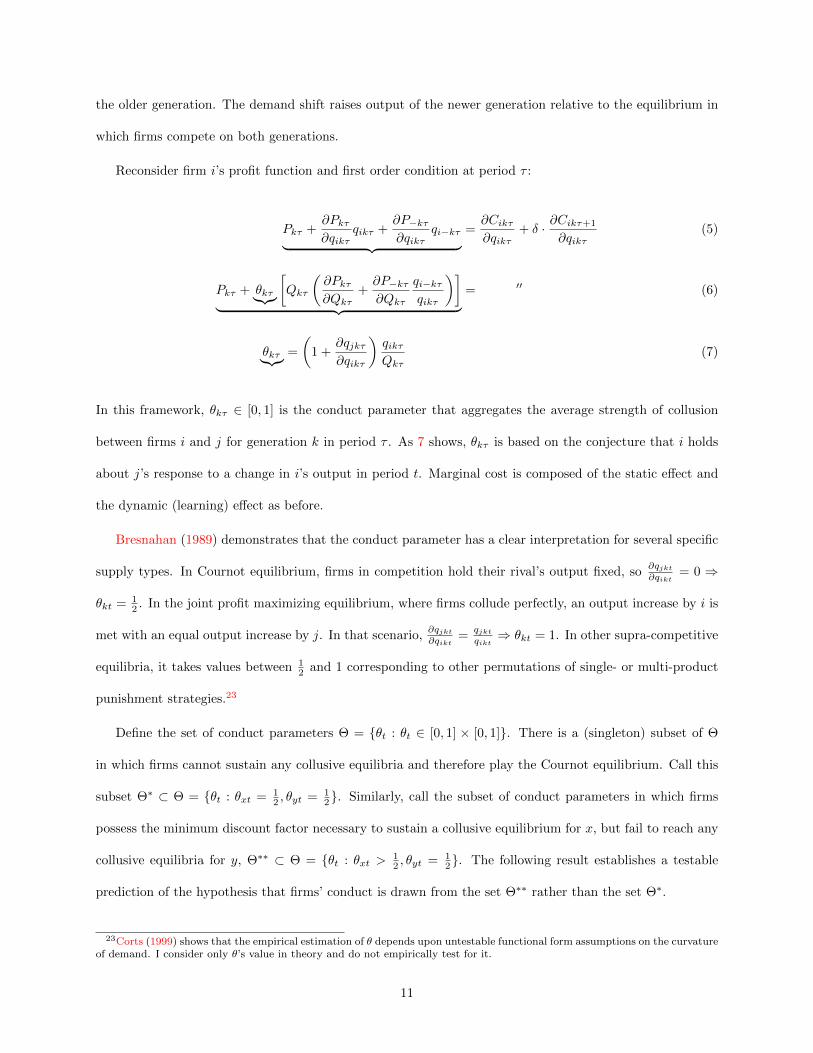
Reconsider firm i’s profit function and first order condition at period τ :

Pkτ +∂Pkτ∂qikτ

qikτ +∂P−kτ∂qikτ

qi−kτ︸ ︷︷ ︸ =∂Cikτ∂qikτ

+ δ · ∂Cikτ+1

∂qikτ(5)

Pkτ + θkτ︸︷︷︸[Qkτ

(∂Pkτ∂Qkτ

+∂P−kτ∂Qkτ

qi−kτqikτ

)]︸ ︷︷ ︸ = ′′ (6)

θkτ︸︷︷︸ =

(1 +

∂qjkτ∂qikτ

)qikτQkτ

(7)

In this framework, θkτ ∈ [0, 1] is the conduct parameter that aggregates the average strength of collusion

between firms i and j for generation k in period τ . As 7 shows, θkτ is based on the conjecture that i holds

about j’s response to a change in i’s output in period t. Marginal cost is composed of the static effect and

the dynamic (learning) effect as before.

Bresnahan (1989) demonstrates that the conduct parameter has a clear interpretation for several specific

supply types. In Cournot equilibrium, firms in competition hold their rival’s output fixed, so∂qjkt∂qikt

= 0 ⇒

θkt = 12 . In the joint profit maximizing equilibrium, where firms collude perfectly, an output increase by i is

met with an equal output increase by j. In that scenario,∂qjkt∂qikt

=qjktqikt⇒ θkt = 1. In other supra-competitive

equilibria, it takes values between 12 and 1 corresponding to other permutations of single- or multi-product

punishment strategies.23

Define the set of conduct parameters Θ = {θt : θt ∈ [0, 1] × [0, 1]}. There is a (singleton) subset of Θ

in which firms cannot sustain any collusive equilibria and therefore play the Cournot equilibrium. Call this

subset Θ∗ ⊂ Θ = {θt : θxt = 12 , θyt = 1

2}. Similarly, call the subset of conduct parameters in which firms

possess the minimum discount factor necessary to sustain a collusive equilibrium for x, but fail to reach any

collusive equilibria for y, Θ∗∗ ⊂ Θ = {θt : θxt >12 , θyt = 1

2}. The following result establishes a testable

prediction of the hypothesis that firms’ conduct is drawn from the set Θ∗∗ rather than the set Θ∗.

23Corts (1999) shows that the empirical estimation of θ depends upon untestable functional form assumptions on the curvatureof demand. I consider only θ’s value in theory and do not empirically test for it.

11

Proposition 2.4.1. Let Ψkt(Θ) be the correspondence from Θ to the set of optimal solutions for firm i on

generation k at time t: Ψkt = {qikt : qikt ∈ argmaxqitπit (qit; st; Θ)}.

Then q∗iyτ ∈ Ψyτ (Θ∗) < q∗∗iyτ ∈ Ψyτ (Θ∗∗) ∀ q∗iyτ , q∗∗iyτ .

Proof 2.4.1. See Appendix C.2.

With empirical data sufficient to identify collusive and non-collusive time periods, Result 2.4.1 constitutes

a testable prediction to bring directly to the data. It examines the consequences of equilibrium output for

generation y at τ if collusion is successful on generation x but unsuccessful on generation y. q∗iyτ denotes i’s

output of y in the baseline Cournot-Nash equilibrium, when firms compete uniformly on both generations.

q∗∗iyτ is i’s output of y in any equilibrium in which firms collude upon x to some degree, but do not collude on

y to any degree. The necessary condition states that industry output for y is greater in the latter equibrium,

when firms are able to collude on x to some degree, than in the former equilibrium, when there is uniform

competition.

The intuition of the result is as follows. When firms reach a collusive equilibrium on x, they internalize

the pecuniaray externality of Cournot competition and therefore cut the output of x relative to the Cournot-

Nash benchmark. Because x is a substitute to y, demand for generation y shifts outward. Firms are unable

to internalize the pecuniary externality on y, so there is an unambiguous increase in the units of y sold.24

Figure 2 depicts the result graphically with linear demand.

[Figure 2 about here.]

In addition, it is important to point out that the possibility of increased output of the new generation at τ

carries significant further dynamic effects. Because of learning-by-doing, ciyτ+1 = c1 · f (qiyτ ) < ciyτ : future

costs decline as a function of current output. When current output increases, firms learn a greater amount

than they otherwise would, which reduces cost in the future. Reduced cost imposes downward pressure on

prices, although it is ambiguous on net whether the price of the newer generation increases or decreases

relative to uniform competition. Lower prices of the newer generation relative to uniform competition are

24If collusion is “more successful” on x than on y, i.e. 12< θyτ < θxτ , the same intuition applies, but the result requires an

additional sufficient condition. Firms face competing output incentives on y: collusion induces them to restrict output, but the

net demand shift is still away from x and toward y. If the cross-price elasticity of demand∂Py∂Qx

< 0 is sufficiently great, the

output expansion effect dominates the output restriction effect.

12

consistent with increased accrued learning through the demand shift described here, and they will also be

tested for in the empirical analysis to follow.

3 DRAM Industry and Market

Semiconductors are crystals—usually silicon—that serve the essential role of connecting the electronic circuits

that make up a microchip. Microchips are a bedrock of the electronics revolution and provide the processing,

memory, speed, and performance ability of computers and many electronic devices. A critical feature of the

microchip is its capacity: the number of transistors per square inch. Increases in capacity reduce the effective

cost of a microchip, or, equivalently, increase its speed. Capacity has risen sharply since the industry’s

inception in the 1970s, famously corresponding to “Moore’s Law”: the maximum capacity of an individual

chip doubles every 18-24 months.

Memory chips store and release data that is used in microprocessor chips such as the computer’s cen-

tral processing unit. DRAM operates at a specific level of the microprocessor by refreshing the transistor

repeatedly. The two chips are complementary: higher processing speed is forfeited unless the device has

enough memory to continuously access data and perform operations. To maximize efficiency, DRAM is sold

as a package of chips attached to a circuit board to create a module. The total capacity of the chips in a

module represents its bit density (“density”), and DRAM product generations are measured by density. Like

most microchips, it is within generations that intensive learning-by-doing takes place.25 DRAM products are

largely homogeneous goods within a density generation, and are substitutable between density generations

based on the customer’s preferences for memory speed.26 Several different density generations are available

at any time, and because of the sequential nature of releases, they are always sequentially ordered between

different points in their life cycles.

The only way to increase capacity is through photolithography, a fabrication process in which hundreds of

chemical reactions are layered onto the underlying silicon wafer that produces microchips.27 While finer-grain

25See Gruber (1998) for evidence of intergenerational learning in EPROM memory chips.26Noll (2014)27The other way to reduce cost per chip—but not capacity per chip—is to increase the size of the wafer itself, which allows

more chips per lithographic batch. Such changes occurred about half as frequently as capacity advancements during the 1980sand 1990s; see Kang (2010) Table 3-2, citing Brown & Linden (2009).

13

etching tools or more complex chemical reactions can advance the lithography process to increase capacity,

they also require very precise light, air and dust conditions. For each duplication in capacity, the new

lithographic process initially produces a yield of zero chips because such conditions are unknown. Producing

a batch of chips requires hundreds of precise steps conducted at the nanoscale level. Engineers continuously

fine tune chemical conditions, employ alternative techniques, phase in higher-technology equipment, and

analyze the resulting data in a trial-by-error process. As Hatch and Mowery (1998) find, the most important

adjustments are in parametric processing, determining the minute range of chemicals to be applied at each

step, followed by adjustments in air particle contamination, which are impacted by the type of lithography

being conducted. Problem diagnoses in these two areas gradually increase numbers of usable chips as

engineers learn which factors are most conducive to functionality and obtain the technical tools to implement

them. Increasing yield drives the cost of each chip down as a direct function of output, consistent with classic

models of learning-by-doing.

In addition to the capacity level, DRAM innovation also occurs along the technology level. Unlike the

capacity innovation process, technology standards are jointly developed by fabricators with input from the

largest microprocessor provider, Intel.28 The JEDEC Solid State Technology Association (“JEDEC”) is

the industry’s Standard Setting Organization, and it typically negotiates technology design, patents and

licensing conditions several years in advance of a new rollout. In the early 2000s, two different types of new

technologies were competing to become the next industry standard. In addition to JEDEC-sponsored Double

Data Rate Synchronous DRAM (“DDR”), the Silicon Valley design firm Rambus developed and patented

Rambus DRAM (“RDRAM”). Appendix B shows that neither technology began to proliferate until after

the cartel period, which rules out the possibility of competition over technologies confounding any of the

empirical cartel results to follow.

The market for DRAM has greatly expanded since its start in the 1970s, primarily through increasing

demand, processing speed and proliferation of computer products. DRAM chips are used directly by orig-

inal equipment manufacturers (OEM’s) for the memory required in personal computer (PC) desktops and

notebooks, and are also purchased as stand-alone products to enhance the memory of existing PC’s.29 For

28Source: private correspondence with Jim Handy, Director at Objective Analysis (May 19, 2014).29Memory manufacturers contract with OEM’s on a biweekly or monthly basis.

14

the data period under study, PC’s were the dominant application of DRAM. They were the only significant

end use throughout the 1980s and early 1990s (Flamm and Reiss, 1993); they comprised about 90% of the

market in the late 1990s and early 2000s (Third Amended Class Action Complaint, MDL No. 1486, pg 76);

and 80% of the market in 2006 (Kang, 2010).30

Because of the large capital outlays for new fabrication plants and variability in demand growth for

computers, the DRAM industry has been highly cyclical since its inception.31 In the late 1990s, the industry

faced significant overcapacity despite steady PC growth.32 After several firms exited the market amid falling

prices and steep losses, in 1998 the largest firms formed a cartel to cut production, raise prices and restore

profitability.33

[Figure 3 about here.]

Figure 3 details the events surrounding the cartel period. After intermittent communication in 1997,

the cartel operated from the second quarter of 1998 through the first quarter of 2001. Noll (2014) relates

that it disbanded when South Korean firm Hynix applied for bankruptcy protection, and restarted after

state-controlled banks bailed out the company for $6-7 billion.34 The cartel ended with DOJ subpoenas in

June 2002 following a public accusation of collusive behavior by the CEO of Dell Inc., Michael Dell.

4 Data

I use a proprietary dataset from industry-leading market research firm Gartner Research that lists quarterly

shipments by firm and density generation, and quarterly market price by density generation, for all firms

in the DRAM market from 1974-2011. I narrow the data to the period for which downstream demand

data is reliably available: 1988-2011. DRAM demand is proxied by a time series of worldwide quarterly

30In recent years, the market for DRAM has begun to shift from traditional PC’s toward mobile smart phones and computertablets, which use lower-power memory but sell many times the units as PC’s. See “Why Growth in Mobile Devices Will FuelMicron’s DRAM Shipments,” Forbes, 1/15/2013 http://www.forbes.com/sites/greatspeculations/2013/01/15/why-growth-

in-mobile-devices-will-fuel-microns-dram-shipments/31Capital depreciation accounted for about 50% of marginal cost in the 1990s and 80% in the 2000s. Source: see Footnote 14.32“But too many new plants were built several years ago in a rush to benefit from a boom many thought would never

end...The glut led to a free fall in prices. In-Stat expects a 21 percent decline in revenue this year, to $15.6 billion.”—DallasMorning News, June 1998 http://articles.chicagotribune.com/1998-06-29/business/9807100053_1_memory-in-personal-

computers-dram-memory-chip-business33See http://europa.eu/rapid/press-release_IP-10-586_en.htm for further information.34“DRAM Rivals Question Korean Government’s Role in Hynix Bailout,” EE Times, 11/5/2001 http://www.eetimes.com/

document.asp?doc_id=1131477.

15

PC shipments obtained from Gartner research reports. This data is available annually from 1988-1996 and

quarterly from 1997-2011.

All prices are given in US dollars and subsequently deflated to year 2000 values by the Consumer Price

Index (CPI). Additionally, the Gartner data includes output per firm by DRAM technology after 2001, when

it began tracking individual technology shipments within generations. Firm names allow accurate tracking

of mergers, entry, and exit throughout the data sample.

In the empirical work to follow, I make use of two subtly different measures of the market price. The

first (employed in previous literature) is the price per module of DRAM generation k sold at time t. Because

DRAM chips are sold as modules, it is the actual price that buyers pay for a given DRAM generation. Another

way to represent DRAM price is through the price of an individual chip standardized by its capacity. The

DRAM price per MB is the market-wide price of a chip divided by its number of megabytes (MB’s). Both

price definitions are equivalent.

[Figure 4 about here.]

Figure 4 plots the price per module by generation for all 11 generations of DRAM from 1988-2011. The

pattern is clear: price is high in initial periods, and it declines in a logarithmic shape as a generation ages.

The most significant price changes occur within the first five to ten years of a generation. This is consistent

with classic models of learning-by-doing.

[Figure 5 about here.]

Figure 5 shows the price per MB averaged and weighted by sales across generations, from 1988-2011.

The standardized price declined through the sample because a fixed DRAM chip becomes cheaper as density

increases. However, there were multiyear cycles of sharp price decreases interspersed with price plateaus

or slight increases. The shaded area represents periods of cartel activity. The figure shows that price

vacillated during the cartel period, staying roughly constant from 1998-2000 before dropping in 2001. The

drop coincides with the period at which the dot-com bubble burst and the cartel disbanded. Price increased

in the first two quarters of 2002, when the cartel regrouped, before declining again after mid-2002 as the

DOJ initiated its investigation.

16

[Figure 6 about here.]

Figure 6 plots the change in aggregate DRAM price per MB against the change in worldwide PC ship-

ments. It shows that most of the variation in DRAM price can be explained by variation in PC shipments.

The effects of the 2001 dot-com bubble crash are particularly striking: both series reach their troughs in

concert. Regression specifications make use of the change in PC shipment rates in explaining generation-level

DRAM price throughout the product life cycle.

Forty-eight different firms appear in the dataset, with a maximum of 24 active firms in 1996.35 As

many as seven different product generations were active at any given cross-sectional point in the dataset,

although two to three accounted for most of the sales.36 Eleven different product generations, from 256Kb

to 2Gb, appear with sufficient frequency to include in the analysis.37 Table E1 lists each DRAM generation

and its years active within the sample period. At the market level, the industry is a classic oligopoly: ten

firms accounted for 85% of output across generations in 2000. The four largest firms—Samsung, Infineon,

Micron, and Hynix—held 63% of the market.38 See Table E2 for C4 concentration ratios by generation from

1994-2004.

5 Empirical Results

The theoretical model presented above generates testable predictions for the effect of collusion on market

prices and outcomes. It is based on the intuition that collusive equilibria are at least as difficult to sustain

on new generations as old generations. The larger is the disparity in average strength of collusion between

generations, the larger is the demand shift toward newer generations. This leads to a sufficient condition

that is testable: newer generations during the cartel period sell more output than they would in competition.

It also implies that the cartel period overcharge is higher for older generations than newer generations, and

ambiguous in sign for newer generations.

35See Siebert and Zulehner (2013) for an empirical analysis of firm entry and shakeout in the DRAM industry.36See fig. F1 for the evolution in market shares between five DRAM generations active during the cartel period.37I also discard two minor “mini-generations,” 2Mb and 8Mb, that briefly appear between industry standard generations in

the 1990s.38I pool the sales of LG Semiconductor with Hynix, which purchased the company in 1999.

17

I provide two types of estimates: (1) the effect of collusion on the dependent variable, output or price; (2)

the effect of collusion on the dependent variable with respect to product cycle age. The first relationship is

identified by repeated product life cycles among generations before, during, and after the cartel. I compare

observations a given amount of quarters from generation or firm entry within the cartel period to other

observations the same amount of quarters from generation or firm entry outside the cartel period, adding a

time-varying proxy for demand.

The second relationship is the differential effect of collusion with respect to generation age. Its identifi-

cation arises from two sources. First, because the cartel was active for 12 quarters, each active generation

provides time-series variation in age. Second, five different generations were at sequentially ordered stages of

their product cycle at each point in time during the cartel. This provides cross-sectional variation between

generations. The latter source is especially strong in ruling out the possibility that changes in firms’ dis-

count factors over time—through macroeconomic conditions, firm-specific financial health or management

changes—bias the results.

5.1 Cartel Output Effects

[Figure 7 about here.]

Figure 7 plots logged generation-level output of DRAM for the first 12 quarters of each generation. It

displays data from the 11 even generations under study, with each dot representing one quarter of output.

Output generally increases from quarter to quarter during the early stage of production, as existing firms

increase their output and new firms enter.

Firms started selling units of 128Mb and 256Mb chips during the cartel period, which is shaded. 128Mb

was the newest generation from 1998 until 1999, when firms began producing 256Mb chips. These two

generations were therefore in the early stage of their product cycles during the cartel period. Sales of the

128Mb and 256Mb generations immediately stand out: initial output values are orders of magnitude greater

than the corresponding values during non-cartel periods before and after the conspiracy.39 It is especially

39Initial output values for the three pre-1982 generations, 4Kb, 16Kb and 64Kb, are also far lower than those for 128Mb and256Mb.

18

noteworthy that 128Mb and 256Mb output is greater than post-cartel generations, because the increasing

market for DRAM over time implies gradually increasing overall output.40

To further investigate the hypothesis that cartel output increased for the newer generations, I estimate

the following regression:

Log(qikt) = β1FirmAgeikt + β2FirmAge2ikt + β3GenAgekt + β4GenAge

2kt

+ β5Yt + β6Yt ×GenAgekt + β7Yt ×GenAge2kt + βk1(Coll)kt + εikt

(8)

This specification regresses the log of a firm’s output for generation k at time t on measures of firm age,

generation age, demand, and an indicator variable for the cartel period. FirmAgeikt and its square denote

the elapsed quarters since firm i began production in generation k. GenAgekt and its square represent the

elapsed quarters since the first firm in generation k began output. These variables account for the positive

trend in output during the early phase of a product cycle, when cost decreases and firms pursue learning

gains, to the negative trend later in the product life cycle, when output crosses its peak and firms shift

production to a newer generation. 1(Coll)kt is an indicator variable equal to one during generation k’s

cartel period and zero otherwise. This variable permits separate estimation of the effect of cartelization on

output by generation.

Yt is a demand shifter representing the growth rate of worldwide PC shipments. Departures from the

baseline rate of PC growth, which is mostly positive through the sample period, are taken as exogeneous

changes in the demand for DRAM.41 Interactions between Yt and GenAgejt allow the effect of a change in

PC shipments to be stronger in the initial phase of a product cycle, when OEM’s may increase production

of memory-intensive computers, than later stages.

[Table 1 about here.]

Table 1 shows that the robust industry-level effect observed in Figure 7 carries over to the firm level

as well. It displays the results of regression 8 with and without controls for demand. The coefficients for

40Figure F3 shows that peak-stage output indeed increases greatly between generations over time.41The proliferation of PC’s from the 1980s through the 2000s was due to the decreasing overall cost of the computer’s

components, of which DRAM only comprises 5-10%. There is no evidence that DRAM prices themselves drive a significantportion of PC sales. See fig. 6 for the correlation between Yt and the aggregate price of DRAM.

19

firm and generation age take the expected signs, with primary terms positive and squared terms negative

signaling the pre- and post-peak phases of the product life cycle. The demand proxies in the right hand side

panel also take the expected signs, with the PC Growth Rate positively associated with output levels at the

earliest stages of the product cycle.

The cartel binary variables are strongly positive and consistent for the 64Mb, 128Mb and 256Mb gen-

erations in both specifications, but negative in the 16Mb generation and negatively significant in the 4Mb

generation. Wald tests for equality reject the joint hypotheses that either of the latter two coefficients arise

from the same distribution as either of the former three coefficients. These results provide strong evidence

that the cartel’s effect was twofold: participants restricted output on older generations and raised output on

newer generations.

5.2 Cartel Price Effects

[Figure 8 about here.]

I now describe and estimate the effect of the DRAM cartel on the price of each active generation. Figure 8

uses DRAM prices per MB to represent all five cartel generations at the same time on the same axis. The

shaded area depicts the cartel period. By inspection, the price of the older, outgoing 4Mb and 16Mb chips

steadily rise, while 64Mb price rises and falls jaggedly to stay roughly equal on average. The prices of the

newer two chips continue to fall.

[Figure 9 about here.]

Figure 9 restricts the price series to the 128Mb and 256Mb generations, which entered during the first

period of collusion and accounted for the majority of market share by the second period. It extends the

x-axis to show the price trend within these generations over the first and second periods of collusion. Prices

decline in the first phase of collusion but rise sharply in the second phase before the cartel is disbanded. The

visual evidence in figures 8 and 9 is consistent with the results of the model: the effect of collusion on price

appears to be larger as the product cycle progresses.

I test this intuition more formally by controlling for the product cycle phase in the following regression.

20

ln(Pjt) = α+ β1LogGenAgejt + β2 Yt + β3 Yt ×GenAgejt + β4 Yt ×GenAge2jt

+ β51(Coll) + εjt

(9)

This regression differs from 8 in two ways. First, the dependent variable ln(Pjt) is the logged industry-level

price of generation k at time t. Second, the regression is run separately for each of the five cartel generations.

The sample for each regression is restricted to a total of 24 quarters before, during, and after the quarters of

cartel activity for the cartel generation in question. This procedure is conducted to maximize the statistical

power of the test because all variation is at the generation-quarter level. 1(Coll) therefore estimates the

average effect of the cartel on the price of k.

[Table 2 about here.]

[Table 3 about here.]

Table 2 and table 3 show the results from regression 9 with and without interactions of DRAM demand

over the product cycle. Generation age enters negatively and significantly in all specifications, consistent with

a decreasing effect of the product cycle phase on price. The coefficients for Yt and its interactions indicate

that the effect of PC growth on DRAM price is positive and significant, that it increases in magnitude in

the ramp-up phase of a product cycle, and that its effect attenuates as a cycle passes its peak.

The second-to-bottom row in all specifications highlights the average effect of collusion on price for

generation k. The estimates are consistent with the model’s predictions: the average effect of collusion on

price appears positively for the 4Mb and 16Mb generations, but significantly lower for the 64Mb, 128Mb

and 256Mb generations.42

In fact, while the collusion coefficient is about 25% and significantly different from zero for the 16Mb

generation, it is negative and significantly different from zero in the 64Mb, 128Mb and 256Mb generations.43

The magnitudes of the price decreases are particularly noteworthy: the 128Mb generation, for example, is

42Figure F2 shows that while the share of generation market share that cartel members comprised was relatively constantand at least 80% for the 16Mb through 256Mb generations, it was only 50% and declining for the 4Mb generation. Insidermarket share declined as the largest firms exited the generation and smaller fringe firms entered. It is therefore unclear whetherto expect a positive or zero effect on cartel price for the 4Mb generation.

43The 256Mb generation entered in Q1-1999. It therefore has only nine quarters of cartel activity.

21

estimated to price 70% lower during the cartel than the competitive counterfactual. The bottom row of

table 3 displays the p-value from a joint test of equality between the collusion coefficient for each generation

and its follower. Equality is rejected strongly for 128Mb, while the p-value ranges from about 10-20% for

64Mb and 256Mb.

These findings lend further credence to table 1’s result that successful collusion on older DRAM genera-

tions shifted demand to newer generations, which produced more during the DRAM cartel than they would

have in competition. They imply that increased output created increased overall learning, and that firms

passed on a component of cost savings to consumers in the 64Mb, 128Mb, and 256Mb generations.

Regression 9 identifies the effect of collusion on price for generation k under the following assumptions:

(1) PC shipment growth affects k and −k’s price equally at equal generation age; (2) supply-side factors

vary as a function of generation age and not time, age-time or age-firm-time. Examples of violations of

(2) include differential levels of capacity utilization between periods (systematic over- or under-capacity) or

tacit collusion in non-cartel periods. If industry-wide changes in supply-side behavior vary over time—and

not over the product cycle—they bias the 1(Collusion) coefficient equally in all five regressions. Because

multiple generations are always on the market at the same time, industry-wide changes apply to generations

at the beginning, middle and end of their product cycles simultaneously.

Regressions of average price level do not capture any time trend in price during the cartel period. If

the rate of price overcharge increases as a function of product age, as the model predicts it does, then the

average price level understates the price effect of collusion. To account for these possibilities, I add a cartel

indicator-age interaction term to regression 9 and display the results below.

[Table 4 about here.]

Table 4 displays empirical results from the specification in which generations are pooled and the cartel

indicator averages across all cartel generations. Results from specifications with and without the 128Mb

generation are consistent with the model’s predictions: the interacted coefficient of cartelization and gener-

ation age is strongly positive and significant. This indicates that the effect of collusion on prices increases

as a function of generation age.

[Figure 10 about here.]

22

Figure 10 plots predicted price coefficients from the model with and without the binary variable indicating

cartel activity. The x-axis is generation age and the y-axis is logged price per module. The figure estimates

the expected price path of a generation beginning collusion from its first period through the rest of its

product cycle. It is consistent with a causal link between collusion in one generation and demand shift

to a preceding generation. Specifically, learning effects through output expansion push the price below its

competitive counterpart for the first 20-24 quarters, while output restriction raises the price in the following

quarters. The break-even point occurs roughly at a generation’s peak in its sixth year.

6 Conclusion

If firms in learning-by-doing industries successfully refrain from competition, the cost to society could be

especially large, because firms would also reduce the rate at which they lower long-term costs. The funda-

mental insight of this paper is that the effectiveness of collusion in such markets is determined by the rate

of learning. The effectiveness of collusion in one product generation impacts equilibrium price and output

of competing product generations. In particular, successful collusion in a mature generation shifts demand

toward newer product generations. If firms are unsuccessful in colluding on newer product generations, the

demand shift induces them to raise output. Increased output results in newer generations learning more

than they would have in a uniformly competitive counterfactual.

Empirical analysis of the DRAM cartel shows evidence consistent with the model. Firms are estimated

to produce substantially more output for the frontier 64Mb, 128Mb and 256Mb generations during collusion

than competiton but less output for the established 4Mb and 16Mb generations. Most interestingly, prices

of the three frontier generations are estimated to be significantly lower as a result of collusion. This implies

that, consistent with the model, firms learned more during 12 quarters of collusion than they would have

during 12 quarters of competition.

It is also noteworthy that these results are not unique to the DRAM market or its episode of collusion.

In the aftermath of the DRAM cartel, many of the largest electronics manufacturers in the world have

settled charges of price fixing in related markets, including LCD panels and hard disk drives. There is strong

evidence that LCD makers, spurred by increased incentives to roll out newer generations, increased the

23

pace of these introductions during collusion relative to competition. Further research and study of different

markets should be conducted to reveal the extent of the substitution and its welfare effects.

This paper carries several implications for antitrust policy, particularly as it relates to many high-

technology industries that experience large cost reductions through learning. Economists have long rec-

ognized that such industries may under- or over-invest in output early in the product cycle depending on the

learning rate, the extent of interfirm learning spillovers, and strategic entry deterrence. The present study

suggests that if firms receive a subsidy or other credit designed to raise their early stage output, they have

strong incentives to pass on the resulting cost savings accrued by learning. These incentives can remain

economically significant even when firms are acting as a cartel.

It further suggests to competition authorities monitoring high-profile, learning-intensive markets that

industry-wide cartelization does not always imply increased prices on all product generations manufactured

by firms in the industry. Indeed, faster-than-usual price decreases may signal collusion among older genera-

tions. Moreover, as technology becomes increasingly expensive to downsize at the nanoscale level, it is well

understood that semiconductors of all types are approaching a limit to cost reduction.44 This means that

overall learning rates are slowing down while other structural features that facilitate coordination—product

homogeneity, multimarket contact, R&D cooperation—remain in place. Competition authorities should be

aware that the conditions favoring shakeout may also raise the likelihood of firms reaching collusive equilibria.

44Mark Bohr, senior fellow and director at Intel, relates: “Everybody in our industry will acknowledge it is getting tougherwith every new generation, [but] we are going to carry the Moore’s Law banner as far as we can.”—“Intel Details 14-NanometerChip Aimed at Tablets,” Wall Street Journal 8/11/2014. http://online.wsj.com/articles/intel-details-new-chip-aimed-

at-tablets-1407775008

24

References

Asker, John. 2010. “A Study of the Internal Organization of a Bidding Cartel.” American Economic

Review, 100(3): 724–762.

Benoit, Jean-Pierre, and Vijay Krishna. 1987. “Dynamic Duopoly: Prices and Quantities.” Review of

Economic Studies, 54(1): 23–35.

Bernheim, Douglas, and Michael D. Whinston. 1990. “Multimarket Contact and Collusive Behavior.”

Rand Journal of Economics, 21(1): 1–26.

Besanko, David, Ulrich Doraszelski, Yaroslav Kryukov, and Mark Satterthwaite. 2010.

“Learning-by-Doing, Organizational Forgetting, and Industry Dynamics.” Econometrica, 78(2): 453–508.

Bolotova, Yuliya, John M. Connor, and Douglas J. Miller. 2008. “The Impact of Collusion on Price

Behavior: Empirical Results from two Recent Cases.” International Journal of Industrial Organization,

26(6): 1290–1307.

Bresnahan, Timothy F. 1989. “Empirical Studies of Industries with Market Power.” In The Handbook

of Industrial Organization. Vol. 2, , ed. Richard Schmalensee and Robert D. Willig, 1011–1057. Elsevier

Science Publishers B. V.

Brod, Andrew, and Ram Shivakumar. 1999. “Advantageous Semi-Collusion.” The Journal of Industrial

Economics, 47(2): 221–230.

Cabral, Luis, and Michael Riordan. 1994. “The Learning Curve, Market Dominance and Predatory

Pricing.” Econometrica, 62(5): 1115–1140.

Cabral, Luis, and Michael Riordan. 1997. “The Learning Curve, Predation, Antitrust, and Welfare.”

The Journal of Industrial Economics, 45(2): 155–169.

Cabral, Ricardo, and Michael J. Leiblein. 2001. “Adoption of a Process Innovation with Learning-by-

Doing: Evidence from the Semiconductor Industry.” The Journal of Industrial Economics, 49(3): 269–280.

25

Clark, Robert, and Jean-Francois Houde. 2013. “Collusion with Asymmetric Retailers: Evidence from

a Gasoline Price-Fixing Case.” American Economic Journal: Microeconomics, 5(3): 97–123.

Clark, Robert, and Jean-Francois Houde. 2014. “The Effect of Explicit Communication on Pricing:

Evidence from the Collapse of a Gasoline Cartel.” The Journal of Industrial Economics, 62(2): 191–228.

Compte, Olivier, Frederic Jenny, and Patrick Rey. 2002. “Capacity Constraints, Mergers and Collu-

sion.” European Economic Review, 46(1): 1–29.

Corts, Kenneth S. 1999. “Conduct Parameters and the Measurement of Market Power.” Journal of Econo-

metrics, 88(2): 227–250.

Dasgupta, Partha, and Joseph Stiglitz. 1988. “Learning-by-Doing, Market Structure and Industrial

and Trade Policies.” Oxford Economics Papers, 40(2): 246–268.

Davidson, Carl, and Raymond Deneckere. 1990. “Excess Capacity and Collusion.” International Eco-

nomic Review, 31(3): 521–541.

Dick, Andrew. 1991. “Learning by Doing and Dumping in the Semiconductor Industry.” Journal of Law

and Economics, 34(1): 133–159.

Fershtman, Chaim, and Ariel Pakes. 2000. “A Dynamic Oligopoly with Collusion and Price Wars.”

The Rand Journal of Economics, 31(2): 207–236.

Flamm, Kenneth, and Peter C. Reiss. 1993. “Semiconductor Dependency and Strategic Trade Policy.”

Brookings Papers on Economic Activity, Microeconomics, , (1): 249–333.

Fudenberg, Drew, and Jean Tirole. 1983. “Learning-by-Doing and Market Performance.” The Bell

Journal of Economics, 14(2): 522–530.

Gardete, Pedro. 2014. “Should Capital-Intensive Firms share Demand Information with Competitors?”

Working Paper, Stanford Graduate School of Business.

Genesove, David, and Wallace P. Mullin. 2001. “Rules, Communication and Collusion: Narrative

Evidence from the Sugar Institute Case.” American Economic Review, 91(3): 379–398.

26

Ghemawat, Pankaj, and Michael A. Spence. 1985. “Learning Curve Spillovers and Market Perfor-

mance.” The Quarterly Journal of Economics, 100: 839–852.

Gruber, Harald. 1998. “Learning-by-Doing and Spillovers: Further Evidence from the Semiconductor

Industry.” Review of Industrial Organization, 13(6): 697–711.

Hatch, Nile W., and David C. Mowery. 1998. “Process Innovation and Learning by Doing in Semicon-

ductor Manufacturing.” Management Science, 44(11): 1461–1477.

Irwin, Douglas A., and Peter J. Klenow. 1994. “Learning-by-Doing and Spillovers in the Semiconductor

Industry.” Journal of Political Economy, 102(6): 1200–1227.

Kang, Joonkyu. 2010. “A Study of the DRAM Industry.” Master’s diss. Massachusetts Institute of Tech-

nology.

Levenstein, Margaret. 1997. “Price Wars and the Stability of Collusion: A Study of the Pre-World War

I Bromine Industry.” The Journal of Industrial Economics, 45(2): 117–137.

Levenstein, Margaret, and Valerie Suslow. 2006. “What Determines Cartel Success?” Journal of

Economic Literature, 44(1): 43–95.

Macher, Jeffrey T., and David C. Mowery. 2003. ““Managing” Learning by Doing: An Empirical Study

in Semiconductor Manufacturing.” The Journal of Product Innovation Management, 20(5): 391–410.

Mariuzzo, Franco, and Patrick Paul Walsh. 2013. “Commodity Market Dynamics and the Joint Ex-

ecutive Committee, 1880-1886.” Review of Economics and Statistics, 95(5): 1722–1739.

Mookherjee, Dilip, and Debraj Ray. 1991. “Collusive Market Structure under Learning-by-Doing and

Increasing Returns.” Review of Economics Studies, 58(5): 993–1009.

Noll, Roger. 2014. “The DRAM Antitrust Litigation.” In The Antitrust Revolution: Economics, Competi-

tion and Policy. . One ed., , ed. John E. Kwoka Jr. and Lawrence J. White, 246–276. Oxford University

Press.

27

Nye, William W. 1996. “Firm-specific Learning-by-Doing in Semiconductor Production: Some Evidence

from the 1986 Trade Agreement.” Review of Industrial Organization, 11(3): 383–394.

Porter, Robert, and Douglas J. Zona. 1999. “Ohio School Milk Markets: an Analysis of Bidding.” The

Rand Journal of Economics, 30(2): 263–288.

Roller, Lars-Hendrik, and Frode Steen. 2006. “On the Workings of a Cartel: Evidence from the

Norwegian Cement Industry.” The American Economic Review, 96(1): 321–338.

Scott Morton, Fiona. 1997. “Entry and Predation: British Shipping Cartels 1879-1929.” Journal of

Economics and Management Strategy, 6(4): 679–724.

Siebert, Ralph. 2010. “Learning-by-Doing and Cannibalization Effects at Multi-Vintage Firms: Evidence

from the Semiconductor Industry.” The B.E. Journal of Economic Analysis & Policy, 10(1): Article 37.

Siebert, Ralph, and Christine Zulehner. 2013. “The Impact of Market Demand and Entry Costs on

Market Structure.” Working Paper, Purdue University Krannert School of Management.

Spence, Michael A. 1981. “The Learning Curve and Competition.” The Bell Journal of Economics,

12(1): 49–70.

Zulehner, Christine. 2003. “Testing Dynamic Oligopolistic Interaction: Evidence from the Semiconductor

Industry.” The International Journal of Industrial Organization, 21(10): 1527–1556.

28

Table 1: Log Firm Output on Covariates, 1988-2011

(1) (2)

Coefficient (Std. Err.) Coefficient (Std. Err.)

Firm Age 0.138∗∗∗ (0.007) 0.143∗∗∗ (0.007)

Firm Age2 -0.002∗∗∗ (0.001) -0.002∗∗∗ (0.001)

Gen Age 0.347∗∗∗ (0.005) 0.348∗∗∗ (0.006)

Gen Age2 -0.004∗∗∗ (0.001) -0.004∗∗∗ (0.001)

PC Growth Rate 0.256∗∗∗ (0.008)

PC Growth Rate × Gen Age -0.013∗∗∗ (0.001)

PC Growth Rate × Gen Age2 0.001∗∗ (0.000)

I(Coll)4 -0.379∗∗∗ (0.101) -0.314∗∗∗ (0.089)

I(Coll)16 -0.117 (0.079) -0.058 (0.073)

I(Coll)64 3.122∗∗∗ (0.191) 2.141∗∗∗ (0.174)

I(Coll)128 4.852∗∗∗ (0.257) 2.569∗∗∗ (0.241)

I(Coll)256 3.743∗∗∗ (0.365) 1.628∗∗∗ (0.335)

R2 0.914 0.9273N 6640 6640

***p < 0.01, **p < 0.05, *p < 0.1. The dependent variable is logged firm-level outputof DRAM units, by quarter. Firm- and generation-age represent the elapsed quarterssince the first firm in generation k began output. I(Coll)k estimates the average changein output for generation k during the cartel period.

29

Table 2: Log Module Price Level on Covariates, 1988-2011

4Mb 16Mb

Intercept 6.360∗∗∗ 5.088∗∗∗ 5.316∗∗∗ 2.841∗∗∗

(0.501) (0.833) (0.496) (0.757)

Log Gen Age -1.551∗∗∗ -1.218∗∗∗ -1.301∗∗∗ -0.597∗∗∗

(0.131) (0.218) (0.141) (0.215)

PC Growth Rate 0.502∗∗ 10.214 1.488∗∗∗ 13.482∗∗

(0.234) (7.124) (0.141) (5.917)

PC Growth Rate × Gen Age -0.367 -0.527(0.313) (0.336)

PC Growth Rate × Gen Age2 0.003 -0.005(0.003) (.005)

I(Collusion) 0.067 0.081 0.243∗∗ 0.262∗∗

(0.077) (0.078) (0.122) (0.120)

Quarters 34-57 34-57 24-47 24-47N 173 173 200 200R2 0.477 0.490 0.350 0.405

***p < 0.01, **p < 0.05, *p < 0.1. The dependent variable is logged industry-level deflatedprice in USD, by generation and quarter. The indicator variable I(Collusion) estimates theaverage price change in the given generation during the cartel period.

30

Table 3: Log Module Price Level on Covariates, 1988-2011

64Mb 128Mb 256Mb

Intercept 7.642∗∗∗ 7.033∗∗∗ 5.651∗∗∗ 5.524∗∗∗ 5.629∗∗∗ 5.494∗∗∗

(0.298) (0.553) (0.234) (0.172) (0.173) (0.233)

Log Gen Age -2.091∗∗∗ -1.882∗∗∗ -1.353∗∗∗ -1.280∗∗∗ -1.335∗∗∗ -1.258∗∗∗

(0.100) (0.189) (0.066) (0.099) (0.066) (0.100)

PC Growth Rate 3.903∗∗∗ 4.933∗ 4.160∗∗∗ 1.865 4.030∗∗∗ 1.740(0.477) (2.965) (0.617) (1.676) (0.621) (1.660)

PC Growth Rate × Gen Age 0.024 0.710∗∗∗ 0.732∗∗∗

(0.291) (0.269) (0.267)

PC Growth Rate × Gen Age2 -0.003 -.034∗∗∗ -.036∗∗∗

(0.007) (0.010) (0.010)

I(Collusion) -0.263∗ -0.289∗ -0.644∗∗∗ -0.701∗∗∗ -0.294 -0.260(0.160) (0.160) (0.197) (0.190) (0.208) (0.199)

2-Sided Eq. Test w/ 4Mb (∗∗) (∗∗∗) ()

2-Sided Eq. Test w/ 16Mb (∗∗∗) (∗∗∗) (∗∗∗)

2-Sided Eq. Test w/ 64Mb (∗) ()

Quarters 7-30 7-30 1-23 1-23 1-23 1-23N 201 201 178 178 178 178R2 0.718 0.722 0.720 0.748 0.720 0.758

***p < 0.01, **p < 0.05, *p < 0.1. The dependent variable is logged industry-level deflated price in USD, by generation and quarter. Theindicator variable I(Collusion) estimates the average price change in the given generation during the cartel period.

31

Table 4: Log Module Price Trend on Covariates, 1988-2011

(1) (2)All Generations 128Mb Omitted

Intercept 5.639∗∗∗ 5.906∗∗∗

(0.117) (0.116)

Log Gen Age -1.382∗∗∗ -1.450∗∗∗

(0.034) (0.034)

PC Growth Rate 5.910∗∗∗ 5.547∗∗∗

(0.584) (0.573)

PC Growth Rate × Gen Age -0.141∗∗∗ -0.136∗∗∗

(0.029) (0.028)

PC Growth Rate × Gen Age2 0.0006∗ 0.001∗∗

(0.0003) (0.0003)

I(Coll) -1.080∗∗∗ -0.912∗∗∗

(0.200) (0.216)

I(Coll) × Log Gen Age 0.334∗∗∗ 0.294∗∗∗

(0.062) (0.065)

N 580 525R2 0.907 0.921

***p < 0.01, **p < 0.05, *p < 0.1. The dependent variable is logged industry-leveldeflated price in USD, by generation and quarter. PC Growth Rate is a demandproxy that measures the year-over-year change in worldwide PC shipments. Inter-actions of PC Growth Rate capture the differential effect of a change in shipmentrates on DRAM price over the early, peak, and post-peak phases of the productcycle. The indicator variable I(Collusion) estimates the average price change fromcartel activity at the first period of a generation’s product cycle. I(Collusion) ×Log Gen Age estimates the price trend from cartel activity during a generation’sproduct cycle.

32

Figure 1: Timing of Product Life Cycles and Learning

33

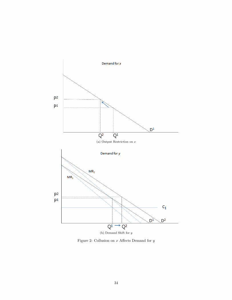
(a) Output Restriction on x

(b) Demand Shift for y

Figure 2: Collusion on x Affects Demand for y

34

Figure 3: Events During Cartel PeriodSources: Noll (2014), DOJ and EC Press Releases, and US Indirect Purchaser litigation

Figure 4: DRAM Module Log Price Trends By Generation

35

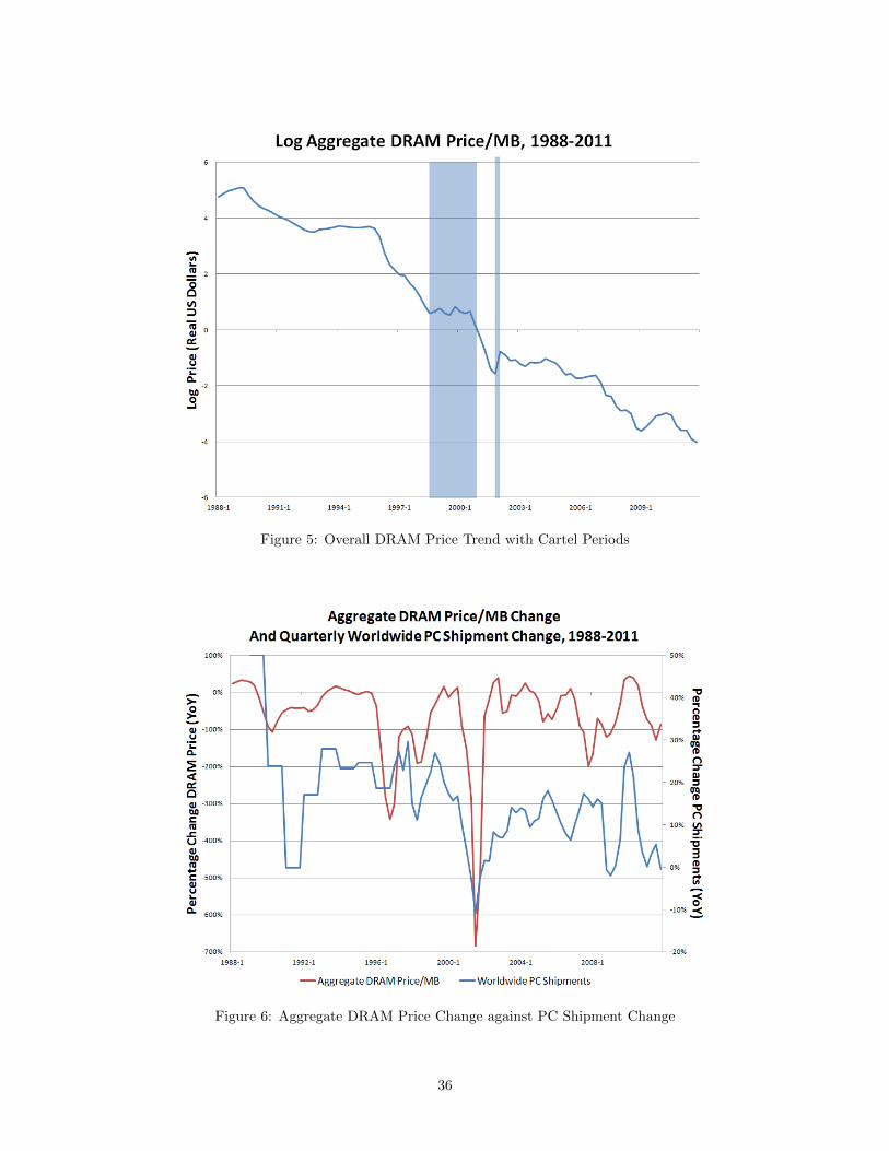
Figure 5: Overall DRAM Price Trend with Cartel Periods

Figure 6: Aggregate DRAM Price Change against PC Shipment Change

36

Figure 7: DRAM Output by Generation, First 12 Quarters

Figure 8: DRAM Price/MB Trend During First Cartel Period

37

Figure 9: DRAM Price/MB Trend From First to Second Cartel Period

Figure 10: Estimated Competitive and Collusive Price Trends

38

Appendices

A Collusion with Multiproduct Punishments

This section allows firms to coordinate collusive strategies across separate product generations linked by

demand substitution.45 It shows that multiproduct punishment may increase the scope for collusion, de-

pending on the level of the firm-invariant discount factor δ, but that collusion is never more sustainable for

x at τ than for y at τ .

Specifically, consider the strategy in which each firm maximizes the discounted sum of joint profits at τ

but punishes deviation in generation k with Cournot reversion in k and −k. Call this strategy σ′′

i . When

punishments occur across generations, firm i will consider either adhering to the collusive path on both

generations or deviating from the collusive path on both generations. Deviation on one and adherence on

the other is strictly dominated by deviation on both, because i knows that deviation on one will be met with

punishment on both generations.

Assume that δ is within the range of interest: δxτ < δ < δyτ . Define the incentive compatibility constri-

ants corresponding to single-product collusion, 3, as gx(δ) and gy(δ) when k = x and k = y, respectively. It

follows that gx(δ) > 0 and gy(δ) < 0.

The only difference between single- and multiproduct punishments is that firms can pool IC constraints

between generations in the multiproduct case. To sustain collusion under σ′′

i , firm i must satisfy:

y∑k=x

∞∑t=τ+1

δt−τ (Π∗∗ikt (·)−Π∗ikt (·)) ≥y∑

k=x

(Π∗ikτ

(q∗ikτ , q

∗∗jkτ , q

∗∗−kτ)−Π∗∗ikτ (·)

)(10)

gx(δ) + gy(δ) ≥ 0 (11)

gx(δ) ≥ −gy(δ) (12)

Pooling IC constraints implies that collusion at the joint profit maximizing value is sustainable only if

the sum of the individual IC constraints across generations (rather than each constraint individually) is

greater than or equal to zero. When δ > δxτ , there is “complementary slack” on the x constraint that can

45The analysis mirrors the treatment of multimarket collusion in Bernheim and Whinston (1990) and subsequent papers.

39

be redistributed to the y constraint. If the slack gx(δ) is sufficiently large relative to (negative) slack −gy(δ),

then this “slack enforcement power” is sufficient to sustain collusion on both generations.

This logic leads to the following result:

Proposition A.1. Defineˆδkt as the minimum discount factor that satisfies σ′′i ’s ICC at t.

If demand is symmetric between generations, fixed across time, and log-linear, then δxτ =ˆδxτ ≤ ˆ

δyτ

Proof A.1.

See Appendix C.1.

Result A.1 shows that under the same sufficient conditions as Proposition 2.3.1, the minimum discount

factor necessary for collusion on x is identical whether the strategy is σ′′

i or σ′

i. The σ′′

i minimum discount

factor for y is bounded to the right by the σ′

i minimum discount factor for y and to the left by the σ′′

i

minimum discount factor for x. Collusion is therefore at least as sustainable for x as it is for y.

With multiproduct punishments, firms can use slack enforcement power from the incentive compatibility

constraint on x to enforce collusion on y only if x’s incentive compatibility constraint has enough slack.

The amount of slack depends on the level of the discount factor. Thus the imbalance between minimum

discount thresholds necessary to sustain collusion may be unchanged, reduced, or completely eliminated. The

scope for successful collusion on one generation and unsuccessful collusion on another generation, however,

is limited to success on x and failure on y.

40

B DRAM Output by Technology

Section 3 describes the rival technologies available to DRAM manufacturers during the early 2000s. DDR,

developed cooperatively by DRAM fabricators through JEDEC, faced a rival technology in RDRAM, licensed

by the design firm Rambus. Although RDRAM boasted slightly faster performance speeds than DDR, the two

technologies were largely substitutable. After initial backing from Intel, RDRAM failed to gain popularity

among fabricators and OEM’s and DDR quickly became the industry standard upon which subsequent

innovations have been based.

The empirical pattern of positive collusive overcharge for the 16Mb and 64Mb generations but zero or

negative overcharges for the 128Mb of 256Mb generations cannot be explained by changes in the underlying

technology of the chips. During the 1990s, the four largest firms—Samsung, Infineon, Micron and Hynix—

designed their plants to accomodate both technology types for 128Mb and 256Mb chips, skipping the older

two generations.46 After DDR became the dominant next-generation technology, Rambus filed a private

antitrust suit in 2004 accusing the DRAM manufacterers of flooding the market with DDR to price out

RDRAM.47. Note that this case is distinct from both the DOJ antitrust case around which this paper

focuses and the string of largely successful Rambus patent infringement suits that spurred the FTC and EC

to file retaliatory “patent ambush” litigation. Figures C1 and C2 rule out the possibility that competition

between firms pushing either of these technologies contributed to the output increase discussed in section 5.1,

because RDRAM and DDR did not proliferate until after 2000:

46“Samsung’s Fuller Disclosure,” Businessweek 11/29/2005 http://www.businessweek.com/stories/2005-11-29/samsungs-

fuller-disclosure47The case proceeded to a $3.95 billion trial in 2011, where a jury ultimately rejected Rambus’ allegation. See “Ram-

bus Loses Antitrust Lawsuit, Shares Plunge,” http://www.reuters.com/article/2011/11/16/us-rambus-micron-verdict-

idUSTRE7AF1XL20111116

41

Figure C1: 128Mb DRAM Technology Share, 1998-2011

Figure C2: 256Mb DRAM Technology Share, 1999-2011

42

C Proofs of Results

C.1 Proof of Proposition 1

Proof 1.

Part I

Separate the ICC for collusion on generations k ∈ {x, y} into three parts, as follows:

δ[(

Π∗∗ikτ+1 (·)−Π∗ikτ+1 (·))]︸ ︷︷ ︸

Part II

+

∞∑t=τ+2

δt−τ (Π∗∗ikt (·)−Π∗ikt (·))︸ ︷︷ ︸Part III

> Π∗ikτ(q∗ikτ , q

∗∗jkτ , q

∗∗−kτ ; st

)−Π∗∗ikτ (·)︸ ︷︷ ︸

Part I

By construction, Part II and Part III are increasing in δ, and it follows that there is a critical discount

factor δkt such that collusion is sustainable for δ ≥ δkt and collusion is unsustainable for δ < δkt.

First, consider Part III. Both generations are in the post-learning phase of their product life cycles, when

cost has reached its minimum c: when k = x, cixt = c; when k = y, ciyt = c. This can be stated as:

[cixt | k = x] = [ciyt | k = y] = c (13)

Symmetric demand between generations x and y implies that:

Pxt +∂Pxt∂qixt

qixt +∂Pyt∂qixt

Qyt

∣∣∣∣ k = x︸ ︷︷ ︸MRxt|k=x

=

Pyt +∂Pyt∂qiyt

qiyt +∂Pxt∂qiyt

Qxt

∣∣∣∣ k = y︸ ︷︷ ︸MRyt|k=y

(14)

Together, 13 and 14 imply the following two equalities:

(q∗xt(·), q∗∗yt (·) | k = x

)=(q∗yt(·), q∗∗xt (·) | k = y

)(q∗∗xt (·), q∗∗yt (·) | k = x

)=(q∗∗yt (·), q∗∗xt (·) | k = y

) (15)

43

Moreover, (13) and (15) imply:

[ Π∗∗ixt (·)−Π∗ixt (·) | k = x ] =[

Π∗∗iyt (·)−Π∗iyt (·) | k = y]∀ t ∈ {τ + 2, . . .} (16)[ ∞∑

t=τ+2

δt−τ (Π∗∗ixt (·)−Π∗ixt (·))∣∣∣∣ k = x

]=

[ ∞∑t=τ+2

δt−τ(Π∗∗iyt (·)−Π∗iyt (·)

) ∣∣∣∣ k = y

](17)

Second, consider Part I. Generation x is at the second phase of its product life cycle, while y is at the

first phase of its life cycle. Therefore cixτ < ciyτ unconditionally, and it follows that:

[ cixτ | k = x ] < [ ciyτ | k = y ] (18)

Despite differential marginal cost across generations, equality of marginal revenues (14) holds.48 This

impiles that the marginal profitability in reducing output is the the same when k = x as it is when k = y:

[∂πixτ∂qixτ

∣∣∣∣ k = x

]=

[∂πiyτ∂qiyτ

∣∣∣∣ k = y

](19)

Furthermore, iso-elastic demand implies that the total profitability in reducing output from the joint profit

maximizing equilibrium to the Cournot equilibrium is the same when k = x as it is when k = y:

[ ∫ q∗ixτ

q∗∗ixτ

∂πixτ∂qixτ

dq

∣∣∣∣ k = x

]=

[ ∫ q∗iyτ

q∗∗iyτ

∂πiyτ∂qiyτ

dq

∣∣∣∣ k = y

](20)

[Π∗ixτ (·)−Π∗∗ixτ (·)

∣∣∣∣ k = x

]=

[Π∗iyτ (·)−Π∗∗iyτ (·)

∣∣∣∣ k = y

](21)

Finally, consider Part II and assume for the sake of contradiction that:

[(Π∗∗ixτ+1 (·)−Π∗ixτ+1 (·)

) ∣∣∣∣ k = x

]=

[(Π∗∗iyτ+1 (·)−Π∗iyτ+1 (·)

) ∣∣∣∣ k = y

](22)

48Note that this also implies that the strategic reaction across generations ∂Qxτ∂Qyτ

=∂Qyτ∂Qxτ

.

44

(22) implies:

[(P ∗∗xτ+1(·)− c

)· q∗∗ixτ+1(·)−

(P ∗xτ+1(·)− c

)· q∗ixτ+1(·)

∣∣∣∣ k = x

]=[(

P ∗∗yτ+1(·)− ciyτ+1

(q∗∗iyτ (·)

))· q∗∗iyτ+1(·)−

(P ∗yτ+1(·)− ciyτ+1

(q∗iyτ (·)

))· q∗iyτ+1(·)

∣∣∣∣ k = y

] (23)

By the same logic as in Part I—cost asymmetry between generations (18) and symmetric iso-elastic

demand—equality (23) implies that ciyτ+1

(q∗∗iyτ (·)

)= ciyτ+1

(q∗iyτ (·)

). However, q∗∗iyτ (·) < q∗iyτ (·) implies:

c1 · f(q∗∗iyτ (·)

)> c1 · f

(q∗iyτ (·)

)(24)

ciyτ+1

(q∗∗iyτ (·)

)> ciyτ+1

(q∗iyτ (·)

)(25)

It follows that the profits from colluding at τ + 1 are greater when k = x than when k = y:

[(Π∗∗ixτ+1 (·)−Π∗ixτ+1 (·)

) ∣∣∣∣ k = x

]<

[(Π∗∗iyτ+1 (·)−Π∗iyτ+1 (·)

) ∣∣∣∣ k = y

](26)

Combining 17, 21, and 26, it follows that the minimum discount factor necessary for collusion when k = x

is lower than the minimum discount factor necessary for collusion when k = y:

δxτ < δyτ � (27)

45

C.2 Proof of Proposition 2

Proof 2.

δ∗J11 < δ∗J22 < δ ⇒

θ1 = θ2 = 1 (28)

[|η1||η1| − 1

− |η1||η1| − 1

2

]>

[|η2||η2| − 1

− |η2||η2| − 1

2

]∀ |ηt| > 1 (29)

∂C∗i∂qi1

[|η1||η1| − 1

− |η1||η1| − 1

2

]>∂Ci∂qi2

[|η2||η2| − 1

− |η2||η2| − 1

2

]∀ |ηt| > 1 (30)

∂C∗i∂qi1

[|η1||η1| − 1

− |η1||η1| − 1

2

]+

(∂C∗J1i

∂qi1− ∂C∗i∂qi1

)|η1||η1| − 1︸ ︷︷ ︸

>0

>∂Ci∂qi2

[|η2||η2| − 1

− |η2||η2| − 1

2

]∀ |ηt| > 1 (31)

∆P1 > ∆P2 (32)

Inequality 29 follows from the assumption that |η1| ≥ |η2|: demand is at least as elastic in period two

as in one. Inequality 30 follows from inequality 29 and the fact that ∂Ci∂qi1

> ∂Ci∂qi2

. Dynamic marginal cost is

higher at period one, when static marginal costs are higher and the learning effect is present, than at period

two, when static marginal costs are lower and the learning effect is not present.49

δ∗J11 < δ < δ∗J22 ⇒

1

2≤ θ1 < θ2 = 1 (33)

∂C∗i (θ1)

∂qi1

[|η1|

|η1| − θ1− |η1||η1| − 1

2

]<∂Ci∂qi2

[|η2||η2| − 1

− |η2||η2| − 1

2

]∀ |ηt| > 1, |η2| − |η1| < ε,

∂C∗i (θ1)

∂qi1− ∂Ci∂qi1

< γ

(34)

49At the first period,∂C∗J1

i∂qi1

≥ ∂C∗i∂qi1

: dynamic marginal cost is higher for collusion than competition. This occurs because

firms in collusion plan to cut period two output relative to the competitive rate, and lower period two output increases theeffective cost of period one output by diminishing its learning advantage.

46

∆P1 < ∆P2 ∀ |ηt| > 1, |η2| − |η1| < ε,∂C∗i (θ1)

∂qi1− ∂Ci∂qi1

<γ (35)

∆P1 > ∆P2 ∀ |ηt| > 1, |η2| − |η1| > ε , or∂C∗i (θ1)

∂qi1− ∂Ci∂qi1

>γ � (36)

The intuition is similar in the above scenario, where conditions for ∆P1 < ∆P2 are derived. The key

step is 33: if the discount factor is high enough to sustain collusion at the joint profit maximizing level at

period two, but not at period one, then θ2 = 1 and θ1 < 1. The remainder of the proof shows that if this

difference in the average strength of collusion is high enough relative to the evolution of dynamic marginal

cost and of price elasticity, then ∆P1 < ∆P2. If not, then ∆P1 > ∆P2.

47

D Additional Tables

Table E1: DRAM Years Activeby Generation, 1974-2011

Generation Years Active∗

4Kb1 1974-1985

16Kb 1976-1985

64Kb 1979-1995

256Kb 1982-1997

1Mb 1985-2002

4Mb 1988-2010

16Mb 1991-2011

64Mb 1996-2011

128Mb 1998-2011

256Mb 1999-2011

512Mb 2001-2011

1Gb 2003-2011

2Gb 2005-2011

4Gb 2010-2011

* Year is counted if at least one firm producesoutput in any quarter1 First year of Gartner data; shipments be-gan about two years earlier

48

Table E2: C4 Concentration Ratios by Generation, 1994-2004∗

Year 16Mb 64Mb 128Mb 256Mb

1994 60.0

1995 51.4 100

1996 51.4 76.3

1997 42.8 79.8

1998 53.4 56.2 100

1999 62.6 67.6 75.1 100

2000 66.8 68.7 76.9 82.6

2001 68.5 73.6 74.3 74.2

2002 60.5 72.2 78.2 77.6

2003 73.7 69.2 79.2 78.4

2004 79.3 70.3 77.0 74.7

* The four largest firms across generations from 1994-2004 were Samsung, In-fineon, Micron and Hynix.In addition to changes in the market shares of the four pre-existing firms, year-to-year changes reflect new firms entering a generation and merger and acqui-sition activity. As characterized in Gartner Research’s data: in 1998, Micronpurchased Texas Instruments’ DRAM operations. In 1999, SK Hynix (thennamed Hyundai) merged with LG Semiconductor. In 2001, NEC and Hitachibegain operating the DRAM joint venture Elpida Memory.

49

E Additional Figures

Figure F1: Revenue Share: 4Mb - 256Mb

50

Figure F2: Cartel Insider Market Share: 4Mb - 256Mb

Figure F3: Total Output by Generation: 256Kb - 4Gb

51