collisions and encounters of stellar...
TRANSCRIPT

8Collisions and Encounters of Stellar
Systems
Our Galaxy and its nearest large neighbor, the spiral galaxy M31, are fallingtowards one another and will probably collide in about 3 Gyr (see Plate 3and Box 3.1).
A collision between our Galaxy and M31 would have devastating conse-quences for the gas in both systems. If a gas cloud from M31 encountered aGalactic cloud, shock waves would be driven into both clouds, heating andcompressing the gas. In the denser parts of the clouds, the compressed post-shock gas would cool rapidly and fragment into new stars. The most massiveof these would heat and ionize much of the remaining gas and ultimately ex-plode as supernovae, thereby shock-heating the gas still further. Dependingon the relative orientation of the velocity vectors of the colliding clouds, thepost-collision remnant might lose much of its orbital angular momentum,and then fall towards the bottom of the potential well of the whole system,thereby enhancing the cloud-collision and star-formation rates still further.We do not yet have a good understanding of this complex chain of events, butthere is strong observational evidence that collisions between gas-rich galax-ies like the Milky Way and M31 cause the extremely high star-formationrates observed in starburst galaxies (§8.5.5).
In contrast to gas clouds, stars emerge unscathed from a galaxy collision.

640 Chapter 8: Collisions and Encounters of Stellar Systems
To see this, consider what would happen to the solar neighborhood in acollision with the disk of M31. According to Table 1.1, the surface density ofvisible stars in the solar neighborhood is ! 30M! pc"2. Assuming that mostof these are similar to the Sun, the number density of stars is N ! 30 pc"2
and the fraction of the area of the galactic disk that is filled by the disks ofthese stars is of order N!R2
! " 5 # 10"14. Thus even if M31 were to scorea direct hit on our Galaxy, the probability that even one of the 1011 stars inM31 would collide with any star in our Galaxy is small.1
However, the distribution of the stars in the two galaxies would be rad-ically changed by such a collision, because the gravitational field of M31would deflect the stars of our Galaxy from their original orbits and viceversa for the stars of M31. In this process, which is closely related to violentrelaxation (§4.10.2), energy is transferred from ordered motion (the relativemotion of the centers of mass of the two galaxies) to random motion. Thusthe collision of two galaxies is inelastic, just as the collision of two lead ballsis inelastic—in both cases, ordered motion is converted to random motion, ofthe stars in one case and the molecules in the other (Holmberg 1941; Alladin1965). Of course, since stars move according to Newton’s laws of motion, thetotal energy of the galactic system is strictly conserved, in contrast to thelead balls where the energy in random motion of the molecules (i.e., heat) iseventually lost as infrared radiation.
A consequence of this inelasticity is that galaxy collisions often lead tomergers, in which the final product of the collision is a single merged stellarsystem. In fact, we believe that both galaxies and larger stellar systems suchas clusters of galaxies are created by a hierarchical or “bottom-up” processin which small stellar systems collide and merge, over and over again, to formever larger systems (§9.2.2).
The most straightforward way to investigate what happens in galaxy en-counters is to simulate the process using an N-body code. Figure 8.1 showsan N-body simulation of the collision of the Galaxy and M31. This is anexample of a major merger, in which the merging galaxies have similarmasses, and the violently changing gravitational field leads to a merger rem-nant that looks quite di!erent from either of its progenitors. In contrast,minor mergers, in which one of the merging galaxies is much smaller thanthe other, leave the larger galaxy relatively unchanged.
Not every close encounter between galaxies leads to a merger. To seethis, let v# be the speed at which galaxy A initially approaches galaxy B andconsider how the energy that is gained by a star in galaxy A depends on v#.As we increase v#, the time required for the two galaxies to pass throughone another decreases. Hence the velocity impulse "v =
!dtg(t) due to the
gravitational field g(t) from galaxy B decreases, and less and less energy istransferred from the relative orbit of the two galaxies to the random motions
1 We have neglected gravitational focusing, which enhances the collision probabilityby a factor of about five but does not alter this conclusion (eq. 7.194).

Introduction 641
Figure 8.1 An N-body simulation of the collision between the Galaxy (bottom) and M31(top) which is expected to occur roughly 3Gyr from now. The simulation follows onlythe evolution of the stars in the two galaxies, not the gas. Each galaxy is represented byroughly 108 stars and dark-matter particles. The viewpoint is from the north Galacticpole. Each panel is 180 kpc across and the interval between frames is 180 Myr. Afterthe initial collision, a open spiral pattern is excited in both disks and long tidal tails areformed. The galaxies move apart by more than 100 kpc and then fall back together fora second collision, quickly forming a remnant surrounded by a complex pattern of shells.The shells then gradually phase mix, eventually leaving a smooth elliptical galaxy. Imageprovided by J. Dubinski (Dubinski, Mihos, & Hernquist 1996; Dubinski & Farah 2006).
of their stars; in fact, when v# is large, |"v| $ 1/v#. Thus, when v#exceeds some critical speed vf , the galaxies complete their interaction withsu#cient orbital energy to make good their escape to infinity. If v# < vf ,the galaxies merge, while if v# % vf the encounter alters both the orbits and

642 Chapter 8: Collisions and Encounters of Stellar Systems
the internal structures of the galaxies only slightly.2 This simple argumentexplains why most galaxies in rich clusters have not merged: although thedensity of galaxies in the clusters is high, so collisions are frequent, therandom velocities of cluster galaxies are so high that the loss of orbital energyin a collision is negligible—the galaxies simply pass through one another, likeghosts.
Until the 1970s, most astronomers believed that collisions betweengalaxies were negligible, except in high-density regions such as clusters. Thisbelief was based on the following argument. The velocities of galaxies arethe sum of the Hubble velocity (eq. 1.13) appropriate to that galaxy’s posi-tion, and a residual, or peculiar velocity. Typical peculiar velocities arevp " 100 km s"1 (Willick et al. 1997). The number density of galaxies is de-scribed by the Schechter law (eq. 1.18), so the density of luminous galaxies(L &> L!) is n " "! " 10"2 Mpc"3. Most of the stars in a typical luminousgalaxy are contained within a radius R " 10 kpc, so the collision cross-sectionbetween two such galaxies is $ " !(2R)2. If the positions and velocities ofthe galaxies are uncorrelated, the rate at which an L! galaxy su!ers collisionswith similar galaxies is then expected to be of order n$vp " 10"6 Gyr"1,so only about one galaxy in 105 would su!er a collision during the age ofthe universe. Such arguments led astronomers to think of galaxies as islanduniverses that formed and lived in isolation.
This estimate of the collision rate turns out to be far too low, for tworeasons. (i) The stars in a galaxy are embedded in a dark halo, which canextend to radii of several hundred kpc. Once two dark halos start to merge,their high-density centers, which contain the stars and other baryonic mat-ter, experience a drag force from dynamical friction (§7.4.4) as they movethrough the common halo. Dynamical friction causes the baryon-rich centralregions to spiral towards the center of the merged halo, where they in turnmerge. Thus the appropriate cross-section is proportional to the square ofthe dark-halo radius rather than the square of the radius of the stellar distri-bution. (ii) As we describe in §9.1, the departures of the matter distributionin the universe from exact homogeneity arose through gravitational forces,and in particular the peculiar velocities of galaxies relative to the Hubbleflow are caused by gravitational forces from nearby galaxies. Consequently,the peculiar velocities of nearby galaxies are correlated—nearby galaxies arefalling towards one another, just like our Galaxy and M31—so the collisionrate is much higher than it would be if the peculiar velocities were ran-domly oriented. In §8.5.6 we show that the merger rate for L! galaxies is& 0.01 Gyr"1, 104 times larger than our naıve estimate.
When two dark halos of unequal size merge, the smaller halo orbitswithin the larger one, on a trajectory that steadily decays through dynamicalfriction. As the orbit decays, the satellite system is subjected to disruptive
2 Thus, galaxies behave somewhat like the toy putty that is elastic at high impactspeeds, but soft and inelastic at low speeds.

8.1 Dynamical friction 643
processes of growing strength. These include steady tidal forces from thehost galaxy, and rapidly varying forces as the smaller halo passes throughthe pericenter of its orbit. As stars are lost from the satellite, they spreadout in long, thin tidal streamers that can provide vivid evidence of ongoingdisruption. Eventually the satellite is completely disrupted, and its stars anddark matter phase-mix with those of the host system.
These processes, which we examine in this chapter, are common to awide variety of astrophysical systems. Dynamical friction (§8.1) drives theorbital evolution not only of satellite galaxies, but also black holes and glob-ular clusters near the centers of galaxies, and bars in barred spiral galaxies.Tidal forces erode satellite galaxies, globular clusters, and galaxies in clus-ters, and also determine the lifetimes of star clusters and wide binary stars.We shall focus on the e!ects of tidal forces in two extreme and analyticallytractable limits: §8.2 is devoted to impulsive tides, which last for only ashort time, while §8.3 examines the e!ects of static tides. §8.4 describes thedynamics of encounters in galactic disks, and their e!ect on the kinematicsof stars in the solar neighborhood. Finally, in §8.5 we summarize and inter-pret the observational evidence for ongoing mergers between galaxies, andestimate the merger rate.
8.1 Dynamical friction
A characteristic feature of collisions of stellar systems is the systematic trans-fer of energy from their relative orbital motion into random motions of theirconstituent particles. This process is simplest to understand in the limitingcase of minor mergers, in which one system is much smaller than the other.
We consider a body of mass M traveling through a population of par-ticles of individual mass ma ' M . Following §1.2.1 we call M the subjectbody and the particles of mass ma field stars. The subject body usually isa small galaxy or other stellar system and thus has non-zero radius, but weshall temporarily assume that it is a point mass. The field stars are mem-bers of a much larger host system of mass M % M , which we assume tobe so large that it can be approximated as infinite and homogeneous. Theinfluence of encounters with the field stars on the subject body can then becharacterized using the di!usion coe#cients derived in §7.4.4. Because thetest body is much more massive than the field stars, the first-order di!u-sion coe#cients D["vi] are much larger than the second-order coe#cientsD["vi"vj ]/v (cf. eqs. 7.83 with m % ma). Thus the dominant e!ect of theencounters is to exert dynamical friction (page 583), which decelerates thesubject body at a rate
dvM
dt= D["v] = (4!G2Mma ln %
"d3va f(va)
vM ( va
|vM ( va|3, (8.1a)

644 Chapter 8: Collisions and Encounters of Stellar Systems
where
% "bmax
b90"
bmaxv2typ
GM% 1 (8.1b)
and b90 is the 90$ deflection radius defined in equation (3.51). Here wehave used equations (7.83), assuming M % ma and adjusting the notationappropriately. The field-star df f(x,va) is normalized so
!d3va f(x,va) =
n(x), where n is the number density of field stars in the vicinity of the subjectbody.
We now estimate the typical value of the factor % in the Coulomblogarithm. When a subject body of mass M orbits in a host system ofmass M % M and radius R, the typical relative velocity is given byv2typ " GM/R. To within a factor of order unity, the maximum impact
parameter bmax " R, where R is the orbital radius of the subject body.Then % " (M/M)(R/R), which is large whenever M ' M, unless thesubject body is very close to the center of the host.
If the subject body has a non-zero radius, the appropriate value for theCoulomb logarithm is modified to
ln % = ln
#bmax
max(rh, GM/v2typ)
$, (8.2)
where rh is the half-mass radius of the subject system (see Problem 8.2).If the field stars have an isotropic velocity distribution,3 equation (7.88)
yields a simpler expression for the dynamical friction,
dvM
dt= (16!2G2Mma ln %
%" vM
0dva v2
af(va)
&vM
v3M
; (8.3)
thus, only stars moving slower than M contribute to the friction. Like anordinary frictional drag, the force described by equation (8.3) always opposesthe motion (dvM/dt is anti-parallel to vM ). Equation (8.3) is usually calledChandrasekhar’s dynamical friction formula (Chandrasekhar 1943a).
If the subject mass is moving slowly, so vM is su#ciently small, we mayreplace f(va) in the integral of equation (8.3) by f(0) to find
dvM
dt! (
16!2
3G2Mma ln %f(0)vM (vM small). (8.4)
Thus at low velocity the drag is proportional to vM—just as in Stokes’s lawfor the drag on a marble falling through honey. On the other hand, forsu#ciently large vM , the integral in equation (8.3) converges to a definitelimit equal to the number density n divided by 4!:
dvM
dt= (4!G2Mman ln %
vM
v3M
(vM large). (8.5)
3 See Problem 8.3 for the case of an ellipsoidal velocity distribution.

8.1 Dynamical friction 645
Figure 8.2 A mass M travels from left to right at speed vM , through a homogeneousMaxwellian distribution of stars with one-dimensional dispersion !. Deflection of the starsby the mass enhances the stellar density downstream, and the gravitational attraction ofthis wake on M leads to dynamical friction. The contours show lines of equal stellardensity in a plane containing the mass M and the velocity vector vM ; the velocities arevM = ! (left panel) and vM = 3! (right panel). The fractional overdensities shown are0.1, 0.2, . . . , 0.9, 1. The unit of length is chosen so that GM/!2 = 1. The shaded circle hasunit radius and is centered at M . The overdensities are computed using equation (8.148),which is based on linear response theory; for a nonlinear treatment see Mulder (1983).
Thus the frictional force falls like vM"2—in contrast to the motion of solid
bodies through fluids, where the drag force grows as the velocity increases.If f(va) is Maxwellian with dispersion #, then equation (8.3) becomes
(cf. eqs. 7.91–7.93)
dvM
dt= (
4!G2Mnm ln %
v3M
%erf(X) (
2X)!
e"X2
&vM , (8.6)
where X * vM/()
2#) and erf is the error function (Appendix C.3). Thisimportant formula illustrates two features of dynamical friction:(i) The frictional drag is proportional to the mass density nm of the stars
being scattered, but independent of the mass of each individual star. Inparticular, if we replace nm in equation (8.6) by the overall backgrounddensity $, we obtain a formula that is equally valid for a host systemcontaining a spectrum of di!erent stellar masses:
dvM
dt= (
4!G2M$ ln %
v3M
%erf(X) (
2X)!
e"X2
&vM . (8.7)
(ii) The frictional acceleration is proportional to M and thus the frictionalforce must be proportional to M 2. It is instructive to consider why

646 Chapter 8: Collisions and Encounters of Stellar Systems
this is so. Stars are deflected by M in such a way that the density ofbackground stars behind M is greater than in front of it (see Figure 8.2and Problem 8.4). The amplitude of this density enhancement or wakeis proportional to M and the gravitational force that it exerts on M isproportional to M times its amplitude. Hence the force is proportionalto M2.
The validity of Chandrasekhar’s formula Although Chandrasekhar’sformula (8.3) was derived for a mass moving through an infinite homogeneousbackground, it can be (and usually is) employed to estimate the drag on asmall body traveling through a much larger host system. In such applicationswe replace f(v) by the value of the df in the vicinity of the small body, vtyp
by the local velocity dispersion, and bmax by the distance of the subject bodyfrom the center of the host. When employed in this way, Chandrasekhar’sformula su!ers from several internal inconsistencies:(i) The choices of bmax and vtyp are rather arbitrary.(ii) We have neglected the self-gravity of the wake. Thus equation (8.3) takes
into account the mutual attraction of M and the background stars, butneglects the attraction of the background stars for each other.
(iii) We obtained equation (8.3) in the approximation that stars move pastM on Keplerian hyperbolae. Orbits in the combined gravitational fieldsof M and the host system would be more complex.
These deficiencies become especially worrisome when M is so large as to becomparable to the mass of the host system that lies interior to M ’s orbit.Nevertheless, N-body simulations and linearized response calculations showthat Chandrasekhar’s formula provides a remarkably accurate description ofthe drag experienced by a body orbiting in a stellar system, usually withina factor of two and often considerably better (Weinberg 1989; Fujii, Funato,& Makino 2006).
The fundamental reasons for this success were discussed in the derivationof the Fokker–Planck equation in §7.4.2, and derive from the large ratiobetween the maximum and minimum impact parameters that contribute tothe Coulomb logarithm ln % = ln(bmax/b90). Consider, for example, a blackhole of mass M = 106 M!, orbiting at radius 1 kpc in a galaxy with velocitydispersion 200 km s"1. Then we may set bmax " 1 kpc and V0 " 200 km s"1,so b90 = 0.1 pc and ln % = 9.2. To address the seriousness of problem (i)above, suppose that we have overestimated bmax by a factor of two, so thecorrect value is only half the orbital radius or 0.5 kpc; then ln % = 8.5, achange of less than 10%. In words, the drag force is insensitive to changesof order unity in bmax and vtyp, because ln % is large. To address problems(ii) and (iii) we note the e!ects of self-gravity are important only on scalescomparable to the Jeans length, which in turn is comparable to bmax. Thusthe e!ects of self-gravity are negligible, and the approximation of a Keplerianhyperbola should be valid, for encounters with impact parameter much lessthan bmax. Suppose then that we consider only encounters with b < 100 pc

8.1 Dynamical friction 647
or 10% of the orbital radius. The contribution to the Coulomb logarithmfrom these encounters is ln(100 pc/b90) = 5.5, a di!erence of only 25% fromour original estimate. In words, most of the total contribution to the dragcomes from encounters with su#ciently small impact parameters that theneglect of self-gravity and the approximation of Keplerian orbits introducenegligible errors.
A more sophisticated treatment of dynamical friction that avoids theinconsistencies of Chandrasekhar’s formula requires the machinery of linearresponse theory that was developed in §5.3. The subject body is regarded asan external potential &e(x, t) that excites a response density in the host sys-tem, governed by the response function R(x,x%, %). We then solve Poisson’sequation to determine the gravitational potential generated by the responsedensity, and the force exerted on the subject body by this response potentialis dynamical friction (Weinberg 1986, 1989).
Like Landau damping, dynamical friction illustrates the curious factthat irreversible processes can occur in a system with reversible equationsof motion. We have seen in §5.5.3 that Landau damping in spherical stellarsystems arises from resonances between the oscillations of the system andthe orbital frequencies of individual stars. Similarly, dynamical friction canbe shown to arise from resonances between the orbital frequencies of thesubject body and the stars (Tremaine & Weinberg 1984b). The rich Fourierspectrum of the gravitational potential from an orbiting point mass ensuresthat many orbital resonances contribute to the drag force, and the cumulativee!ect of these many weak resonances gives rise to the Coulomb logarithm inChandrasekhar’s formula.
8.1.1 Applications of dynamical friction
(a) Decay of black-hole orbits The centers of galaxies often containblack holes with masses 106–109M! (§1.1.6). It is natural to ask whethersuch objects could be also be present at other locations in the galaxy, wherethey would be even harder to find. To investigate this question, we imaginea black hole of mass M on a circular orbit of radius r, and ask how long isneeded for dynamical friction to drag the black hole to the galaxy center.
The flatness of many observed rotation curves suggests that we approx-imate the density distribution by a singular isothermal sphere (eq. 4.103),
$(r) =v2c
4!Gr2, (8.8)
where vc =)
2# is the constant circular speed (eq. 4.104). The df of theisothermal sphere is Maxwellian, so equation (8.7) gives the frictional force

648 Chapter 8: Collisions and Encounters of Stellar Systems
'F = M |dvM/dt| on the black hole:
'F =4!G2M2$(r) ln %
v2c
%erf(X) (
2X)!
e"X2
&
= 0.428 ln%GM2
r2,
(8.9)
where X = vc/()
2#) = 1.This force is tangential and directed opposite to the velocity of the black
hole, causing it to lose angular momentum 'L at a rate
d'Ldt
= ( 'Fr ! (0.428 ln%GM2
r. (8.10)
Thus the black hole spirals towards the center of the galaxy, while remain-ing on a nearly circular orbit. Since the circular-speed curve of the singularisothermal sphere is flat, the black hole continues to orbit at speed vc as itspirals inward, so its angular momentum at radius r is 'L = Mrvc. Substi-tuting the time derivative of this expression into equation (8.10), we obtain
rdr
dt= (0.428 ln%
GM
vc= (0.302 ln%
GM
#. (8.11)
If we neglect the slow variation of ln % with radius, we can solve this di!er-ential equation subject to the initial condition that the radius is ri at zerotime. We find that the black hole reaches the center after a time4
tfric =1.65
ln %
r2i #
GM=
19 Gyr
ln %
#ri
5 kpc
$2 #
200 km s"1
108 M!
M. (8.12)
This equation can be cast into a simpler form using the crossing time tcross =ri/vc, the time required for the subject body to travel one radian,
tfric =1.17
ln %
M(r)
Mtcross, (8.13)
where M(r) = v2c r/G is the mass of the host galaxy contained within radius
r. This result is approximately correct even for mass distributions otherthan the singular isothermal sphere; in words, if the ratio of the mass of thesubject body to the interior mass of the host is µ ' 1, then the subject bodyspirals to the center of the host in roughly 1/(µ ln %) initial crossing times.
For characteristic values bmax " 5 kpc, M = 108 M!, and vtyp " # =200 km s"1, we have by equation (8.1b) that ln % ! 6. Thus for the standard
4 Equation (8.8) overestimates the density inside the galaxy’s core, but this leads to anegligible error in the inspiral time, since the decay is rapid at small radii anyway.

8.1 Dynamical friction 649
parameters in equation (8.12), the inspiral time tfric is only 3 Gyr. Black holeson eccentric orbits have even shorter inspiral times than those on circularorbits with the same mean radius, since the eccentric orbit passes throughregions of higher density where the drag force is stronger. We conclude thatany 108 M! black hole that is formed within & 10 kpc of the center of atypical galaxy will spiral to the center within the age of the universe. Thusmassive black holes should normally be found at the center of the galaxy,unless they are far out in the galactic halo.
(b) Galactic cannibalism Most large galaxies are accompanied by sev-eral satellite galaxies, small companion galaxies that travel on bound orbitsin the gravitational potential of the larger host. The satellites of our ownMilky Way galaxy include the Sagittarius dwarf galaxy, the Large and SmallMagellanic Clouds (§1.1.3 and Plate 11), and several dozen even smallergalaxies at distances of & 100–300 kpc. Two satellite galaxies of the nearbydisk galaxy M31 appear in Plate 3.
Satellites orbiting within the extended dark halo of their host experiencedynamical friction, leading to orbital decay. As the satellite orbit decays,tidal forces from the host galaxy (§8.3) strip stars from the outer parts ofthe satellite, until eventually the entire satellite galaxy is disrupted—thisprocess, in which a galaxy consumes its smaller neighbors, is an example ofa minor merger, or, more colorfully, galactic cannibalism.
The rate of orbital decay for a satellite of fixed mass M is describedapproximately by equation (8.12). This formula does not, however, allow formass loss due to tidal stripping as the satellite spirals inward. To accountcrudely for this process, we shall refer forward to §8.3, in which we show thatthe outer or tidal radius of a satellite is given approximately by its Jacobiradius rJ, defined by equation (8.91). Once again we assume that the hostgalaxy is a singular isothermal sphere, so its mass interior to radius r isM(r) = v2
Mr/G = 2#2Mr/G, where vM and #M = vM/
)2 are the circular
speed and velocity dispersion of the host; in this case equations (8.91) and(8.108) yield
rJ =
#M
2M(r)
$1/3
r =
#GMr2
4#2M
$1/3
. (8.14)
We shall assume that the satellite galaxy is also a singular isothermal sphere,but one that is sharply truncated at rJ. Thus the total mass of the satellite isM = 2#2
s rJ/G, where #s is its velocity dispersion. (A truncated isothermalsphere is not a self-consistent solution of the collisionless Boltzmann andPoisson equations, so this should be regarded as a fitting formula withoutmuch dynamical significance.) Equation (8.14) then yields
rJ =#s)2#M
r which implies that M =
)2#3
s r
G#M. (8.15)

650 Chapter 8: Collisions and Encounters of Stellar Systems
Substituting into equation (8.11), we obtain the rate of orbital decay,
dr
dt= (0.428 ln%
#3s
#2M
, (8.16)
and neglecting the slow variation in ln % with radius, we find the inspiraltime from radius ri to be
tfric =2.34
ln %
#2M#3
s
ri
=2.7 Gyr
ln %
ri
30 kpc
( #M
200 km s"1
)2#
100 km s"1
#s
$3
.
(8.17)
To evaluate the Coulomb logarithm, we use equation (8.2). The half-massradius rh of the satellite is half of its Jacobi radius, and the typical velocitymay be taken to be vtyp = #M. Then the two quantities in the denominatorof equation (8.2) are given by equations (8.15),
rh =#s
23/2#Mr ;
GM
v2typ
=
)2#3
s
#3M
r. (8.18)
The velocity dispersion of a galaxy is correlated with its mass through theFaber–Jackson law (1.21). Satellite galaxies have smaller luminosities thantheir hosts, and hence smaller dispersions. If #s &< 0.5#M, the first term inequation (8.18) is larger than the second, so the argument of the Coulomblogarithm is % = bmax/rh; setting bmax = r we have finally % = 23/2#M/#s.Thus, for example, equation (8.17) implies that in a host galaxy with disper-sion 200 km s"1, a satellite galaxy with dispersion # &> 50 km s"1 will mergefrom a circular orbit with radius 30 kpc within 10 Gyr.
(c) Orbital decay of the Magellanic Clouds In general, the orbits ofsatellites of the Milky Way cannot be determined, because their velocitiesperpendicular to the line of sight are either unknown or have large obser-vational uncertainties. However, much more information is available for theLarge and Small Magellanic Clouds. Not only do we have good estimates fortheir velocities perpendicular to the line of sight (Kallivayalil et al. 2006),but the correct Cloud orbits must be able to reproduce the dynamics of theMagellanic Stream, a narrow band of neutral hydrogen gas that extends over120$ in the sky and is believed to have been torn o! the Small Cloud by thegravitational field of the Galaxy about 1–1.5 Gyr ago. (See BM §8.4.1 andPutman et al. 2003 for a description of the observations.)
Several groups have modeled the dynamics of the Magellanic Streamand the resulting constraints on the Cloud orbits (Murai & Fujimoto 1980;Lin & Lynden–Bell 1982; Gardiner, Sawa, & Fujimoto 1994; Connors et al.2004). They find that the orbital plane of the Clouds is nearly perpendicular

8.1 Dynamical friction 651
Figure 8.3 The decay of the orbits of the Magellanic Clouds around our Galaxy. Theupper curves show the radius of the Clouds from the Galactic center (thick line for theLarge Cloud and thin line for the Small Cloud), and the lower, dashed curve shows thedistance between the Large and Small Cloud. The Galaxy potential is that of a singularisothermal sphere with circular speed vc = 220 km s!1, and the drag force is computedusing Chandrasekhar’s formula (8.7). The initial conditions at t = 0 are chosen to repro-duce the observed distances and radial velocities of the Clouds and the kinematics of theMagellanic Stream (Gardiner, Sawa, & Fujimoto 1994).
to the Galactic plane; the sense of the orbit is such that the Clouds areapproaching the Galactic plane with the Magellanic Stream trailing behind;the orbit is eccentric (the apocenter/pericenter distance is &> 2); and theClouds are presently near pericenter (Figure 8.3). As seen in the figure, theorbits of the Magellanic Clouds are decaying due to dynamical friction. Theongoing mass loss from the Clouds that generates the Magellanic Streamprovides circumstantial evidence that the orbit is continuing to shrink.
In this model the Clouds merge with the Milky Way in about 6 Gyr,although the model is unrealistic beyond about 3 Gyr in the future, whenthe Galaxy experiences a much more violent merger with M31 (Box 3.1).
(d) Dynamical friction on bars Dynamical friction can be generatedby any time-varying large-scale gravitational field. An important example isthe interaction between a bar in a disk galaxy and the surrounding dark halo.As a first approximation, let us think of the bar as a rigid body, consisting

652 Chapter 8: Collisions and Encounters of Stellar Systems
of two masses M at the ends of a rod of length 2r that revolves aroundits center at the bar pattern speed 'b. In a strong bar M would not bemuch smaller than the mass of the galaxy interior to r. In this circumstanceequation (8.13) suggests that the bar should lose its angular momentum in afew crossing times, which is much shorter than the age of the galaxy. Thuswe might expect that bars in disk galaxies with massive halos would havezero angular momentum and zero pattern speed.
Improving on this crude model is a challenging analytic task, for sev-eral reasons: first, the gravitational potential of a bar is more complicatedthan the potential from a point mass; second, in contrast to most orbitingbodies, bars are extended objects, so the friction is not dominated by localencounters; third, dynamical friction exerts a torque on the bar but we donot understand the reaction of the bar to that torque: does its pattern speedincrease or decrease? does the bar grow stronger or weaker? etc.
Accurate analytic determinations of the frictional torque on a bar fromthe dark halo can be derived using perturbation theory (Weinberg 1985),but N-body simulations can be more informative because they determineboth the torque on the bar and its resulting evolution. Simulations confirmthat the halo exerts a strong frictional torque on the bar, and show that inresponse the bar pattern speed rapidly decays but the bar remains intact(Sellwood 1980; Hernquist & Weinberg 1992; Debattista & Sellwood 1998,2000).
These theoretical results imply that if massive dark halos are present inthe inner parts of barred galaxies, bars should rotate slowly. However, thisconclusion is inconsistent with observations: as we saw in §6.5.1a the ratio Rof the corotation radius to the bar semi-major axis (eq. 6.103) generally liesin the range 0.9–1.3, where R ! 1 is the maximum allowed rotation rate fora weak bar. This problem can be resolved if spiral galaxies have maximumdisks (§6.3.4), for then the halo mass is relatively small in the inner few kpc,where interactions with the bar are strongest.
(e) Formation and evolution of binary black holes Since most galax-ies contain black holes at their centers, it is natural to ask what happens tothe black holes when a satellite galaxy merges with a larger host.
As the satellite’s orbit decays, its stars are stripped by tidal forces thatbecome stronger and stronger as the orbit shrinks (eq. 8.15), until eventuallyonly its central black hole is left. The orbit of the black hole continues todecay from dynamical friction, although at a slower rate since the mass ofthe black hole is only a small fraction of the mass of the original satellitegalaxy. Assuming that the host galaxy also contains a central black hole, weexpect that eventually the two black holes will form a bound binary system.
After the black-hole binary is formed, its orbit continues to decay by dy-namical friction. Equation (8.3) still describes the drag acting on each blackhole, with the maximum impact parameter bmax appearing in the Coulomblogarithm now equal to the binary semi-major axis a.

8.1 Dynamical friction 653
As the binary orbit shrinks, the relative orbital velocity v of the twoblack holes grows. Eventually the orbital velocity greatly exceeds the velocitydispersion # of the stars in the galaxy. For a circular orbit, this occurs whenthe binary semi-major axis a satisfies
G(M1 + M2)
a% #2 or a ' 10 pc
M1 + M2
108 M!
#200 km s"1
#
$2
, (8.19)
where M1 and M2 are the masses of the black holes. Following the discussionin §7.5.7, we shall say that the black-hole binary is hard when v > #.
For hard binaries Chandrasekhar’s dynamical friction formula is nolonger valid, but an approximate formula for the rate of orbital decay can bederived by arguments similar to those used to derive the hardening rate forbinary stars in equation (7.179). These yield (Quinlan 1996b)
d
dt
#1
a
$= (C
G$
#, C = 14.3, (8.20)
where $ is the density of stars in the vicinity of the binary. This result isalmost independent of the eccentricity of the binary and depends only weaklyon the mass ratio M2/M1 so long as it is not too far from unity.5
Under the assumption that the galaxy has a constant-density core, wecan integrate equation (8.20) to obtain 1/a = constant (CG$t/#. Choosingthe origin of time so that the constant is zero, we obtain a = #/(CG$t).The King radius of the galaxy, r0, is related to $ and # via 4!G$r2
0 = 9#2
(eq. 4.106). Eliminating $ with the help of this equation, we have finally
a(t) =4!r2
0
9C#t= 0.005 pc
200 km s"1
#
#r0
100 pc
$2 Gyr
t. (8.21)
Thus interactions with stars in the host galaxy can drive the black-holebinary to semi-major axes as small as a few milliparsecs; the correspondingrelative speed for a circular orbit is
v =
*G(M1 + M2)
a= 2.1 # 104 km s"1
#M1 + M2
108 M!
10"3 pc
a
$1/2
. (8.22)
There is an important case in which this analysis fails. Only stars withangular momentum L &< [G(M1 +M2)a]1/2 interact strongly with the binary,and if the binary semi-major axis a is much smaller than the King radius r0
then this is much smaller than the typical angular momentum L & r0# of
5 The numerical coe!cient di"ers from the one in equation (7.179) because here thebinary components are much more massive than the field stars, while in equation (7.179)the binary components and the field stars all have the same mass.

654 Chapter 8: Collisions and Encounters of Stellar Systems
stars in the core. Thus, only a small fraction of the stars in the core interactstrongly with the black holes. The region in phase space with such smallangular momentum is called the loss cone, by analogy with the loss conefrom which stars are consumed by a single black hole (§7.5.9). The mass ofstars in the loss cone shrinks as the binary semi-major axis decreases, andeventually may become smaller than the black-hole mass. In this case thebinary can empty the loss cone, and the shrinkage of the semi-major axis willstall. Once the loss cone has been emptied, the rate of continued evolutionis much less certain, being determined by the rate at which the loss cone isslowly refilled by two processes: di!usion of angular momentum due to two-body relaxation (Chapter 7), or torques from the host galaxy, if its overallmass distribution is non-spherical (Yu 2002; Makino & Funato 2004).
If the binary semi-major axis shrinks far enough, gravitational radiationtakes over as the dominant cause of orbital decay. A binary black hole ona circular orbit with semi-major axis a will coalesce under the influence ofgravitational radiation in a time (Peters 1964)
tgr =5c5a4
256G3M1M2(M1 + M2)
= 5.81 Myr
#a
0.01 pc
$4 #108 M!
M1 + M2
$3(M1 + M2)2
M1M2.
(8.23)
The characteristic decay time due to gravitational radiation therefore scalesas a4. In contrast, the decay time (d ln a/dt)"1 due to dynamical frictionvaries as 1/a. Consequently, the actual decay time, which is set by the moree#cient of the two processes, has a maximum at the semi-major axis wherethe two decay times are equal (Begelman, Blandford & Rees 1980). Thisradius is referred to as the bottleneck radius, and lies between 0.003 pcand 3 pc depending on the galaxy density distribution and black-hole masses(Yu 2002). The bottleneck radius is where binary black holes are most likelyto be found.
The decay time at the bottleneck is quite uncertain, since it dependson both the extent to which the loss cone is depopulated, and the possiblecontribution of gas drag. If the bottleneck decay time exceeds 10 Gyr, mostgalaxies should contain binary black holes at their centers. If the decaytime is less than 10 Gyr, most black-hole binaries will eventually coalesce.Coalescing black holes are of great interest because they generate strongbursts of gravitational radiation that should ultimately be detectable, evenat cosmological distances, and thus provide a unique probe of both galaxyevolution and general relativity.
(f) Globular clusters These systems may experience significant orbitaldecay from dynamical friction. The rate of decay and inspiral time can bedescribed approximately by equations (8.11) and (8.12). For a typical cluster

8.2 High-speed encounters 655
mass M = 2 # 105 M! (Table 1.3) the inspiral time from radius ri is
tfric = 64 Gyr#
200 km s"1
#ri
1 kpc
$2
, (8.24)
where # is the velocity dispersion of the host galaxy and we have assumedln % = 5.8, from equation (8.2) with bmax = 1 kpc and rh = 3 pc (Table 1.3).Orbital decay is most important for low-luminosity host galaxies, which havesmall radii and low velocity dispersions. Many dwarf elliptical galaxies ex-hibit a deficit of clusters near their centers and compact stellar nuclei, whichmay arise from the inspiral and merger of these clusters (Lotz et al. 2001).A puzzling exception is the Fornax dwarf spheroidal galaxy, a satellite of theMilky Way, which contains five globular clusters despite an estimated inspi-ral time of only tfric & 1 Gyr (Tremaine 1976a). Why these clusters have notmerged at the center of Fornax remains an unsolved problem.
8.2 High-speed encounters
One of the most important classes of interaction between stellar systemsis high-speed encounters. By “high-speed” we mean that the duration ofthe encounter—the interval during which the mutual gravitational forces aresignificant—is short compared to the crossing time within each system. Atypical example is the collision of two galaxies in a rich cluster of galaxies(§1.1.5). The duration of the encounter is roughly the time it takes the twogalaxies to pass through one another; given a galaxy size r & 10 kpc and thetypical encounter speed in a rich cluster, V " 2000 km s"1, the duration isr/V " 5 Myr. For comparison the internal dispersion of a large galaxy is# " 200 km s"1 so the crossing time is r/# " 50 Myr, a factor of ten larger.
As we saw at the beginning of this chapter, the e!ect of an encounteron the internal structure of a stellar system decreases as the encounter speedincreases. Hence high-speed encounters can be treated as small perturbationsof otherwise steady-state systems.
We consider an encounter between a stellar system of mass Ms, thesubject system, and a passing perturber—a galaxy, gas cloud, dark halo,black hole, etc.—of mass Mp. At the instant of closest approach, the centersof the subject system and the perturber are separated by distance b and haverelative speed V . If the relative speed is high enough, then:(i) The kinetic energy of relative motion of the two systems is much larger
than their mutual potential energy, so the centers travel at nearly uni-form velocity throughout the encounter.
(ii) In the course of the encounter, the majority of stars will barely movefrom their initial locations with respect to the system center. Thus the

656 Chapter 8: Collisions and Encounters of Stellar Systems
gravitational force from the perturber can be approximated as an im-pulse of very short duration, which changes the velocity but not the po-sition of each star. A variety of analytic arguments (see page 658) andnumerical experiments (Aguilar & White 1985) suggest that this im-pulse approximation yields remarkably accurate results, even whenthe duration of the encounter is almost as long as the crossing time.6
We now ask how the structure of the subject system is changed by the passageof the perturber. We work in a frame that is centered on the center of massof the subject system before the encounter. Let m" be the mass of the &thstar of the subject system, and let v%
" be the rate of change in its velocitydue to the force from the perturber. We break v%
" into two components. Thecomponent that reflects the rate of change of the center-of-mass velocity ofthe subject system is
vcm *1
Ms
+
#
m#v%# , where Ms *
+
#
m# (8.25a)
is the mass of the subject system. The component
v" * v%" ( vcm (8.25b)
gives the acceleration of the &th star with respect to the center of mass.Let &(x, t) be the gravitational potential due to the perturber. Then
v%" = (!&(x", t), (8.26)
and equation (8.25b) can be written
v" = (!&(x", t) +1
Ms
+
#
m#!&(x# , t). (8.27)
In the impulse approximation, x" is constant during an impulsive en-counter, so
"v" =
" #
"#dt v" =
" #
"#dt
%(!&(x", t)+
1
Ms
+
#
m#!&(x# , t)
&. (8.28)
The potential energy of the subject system does not change during the en-counter, so in the center-of-mass frame the change in the energy, 'E, is simply
6 Condition (ii) almost always implies condition (i), but condition (i) need not implycondition (ii): for example, a star passing by the Sun at a relative velocity v ! 50 km s!1
and an impact parameter b ! 0.01 pc will hardly be deflected at all and hence satisfiescondition (i). However, the encounter time b/v ! 200 yr is much larger than the orbitalperiod of most of the planets so the encounter is adiabatic, rather than impulsive.

8.2 High-speed encounters 657
the change in the internal kinetic energy, 'K. Here tildes on the symbols area reminder that these quantities have units of mass#(velocity)2, in contrastto the usual practice in this book where E and K denote energy per unitmass. We have
" 'E = " 'K = 12
+
"
m"
,(v" + "v")2 ( v2
"
-
= 12
+
"
m"
,|"v"|2 + 2v" · "v"
-.
(8.29)
In any static axisymmetric system,.
" m"v" · "v" = 0 by symmetry (seeProblem 8.5). Thus the energy changes that are first-order in the smallquantity "v average to zero, and the change of internal energy is given bythe second-order quantity
" 'E = " 'K = 12
+
"
m"|"v"|2. (8.30)
This simple derivation masks several subtleties:
(a) Mass loss Equation (8.29) shows that the encounter redistributes aportion of the system’s original energy stock: stars in which v" · "v" > 0gain energy, while those with v" · "v" < 0 may lose energy. The energygained by some stars may be so large that they escape from the system,and then the overall change in energy of the stars that remain bound can benegative. Thus the energy per unit mass of the bound remnant system maydecrease (become more negative) as the result of the encounter, even thoughthe encounter always adds energy to the original system.
(b) Return to equilibrium After the increments (8.28) have been addedto the velocities of all the stars of the subject system, it no longer satisfies thevirial theorem (4.250). Hence the encounter initiates a period of readjust-ment, lasting a few crossing times, during which the subject system settlesto a new equilibrium configuration.
If the perturbation is weak enough that no stars escape, some propertiesof this new equilibrium can be deduced using the virial theorem. Let theinitial internal kinetic and total energies be 'K0 and 'E0, respectively. Thenthe virial theorem implies that
'K0 = ( 'E0. (8.31)
Since the impulsive encounter increases the kinetic energy by " 'K and leavesthe potential energy unchanged, the final energy is
'E1 = 'E0 + " 'K. (8.32)

658 Chapter 8: Collisions and Encounters of Stellar Systems
Once the subject system has settled to a new equilibrium state, the finalkinetic energy is given by the virial theorem,
'K1 = ( 'E1 = (( 'E0 + " 'K) = 'K0 ( " 'K. (8.33)
Thus if the impulsive encounter increases the kinetic energy by " 'K, thesubsequent relaxation back to dynamical equilibrium decreases the kineticenergy by 2" 'K!
(c) Adiabatic invariance The impulse approximation is valid only ifthe encounter time is short compared to the crossing time. In most stellarsystems the crossing time is a strong function of energy or mean orbitalradius, so the impulse approximation is unlikely to hold for stars near thecenter. Indeed, su#ciently close to the center, the crossing times of moststars may be so short that their orbits deform adiabatically as the perturberapproaches (§3.6.2c). In this case, changes that occur in the structure of theorbits as the perturber approaches will be reversed as it departs, and theencounter will leave most orbits in the central region unchanged.
If we approximate the potential near the center of the stellar systemas that of a harmonic oscillator with frequency ', then the energy changeimparted to the stars in an encounter of duration % is proportional toexp((&'%) for '% % 1, where & is a constant of order unity (see §3.6.2a).However, this strong exponential dependence does not generally hold in re-alistic stellar systems. The reason is that some of the stars are in resonancewith the slowly varying perturbing force, in the sense that m·! ! 0 where thecomponents of !(J) are the fundamental frequencies of the orbit (eq. 3.190),and m is an integer triple. At such a resonance, the response to a slowexternal perturbation is large—in the language of Chapter 5, the polariza-tion matrix diverges (eq. 5.95). A careful calculation of the contribution ofboth resonant and non-resonant stars shows that the total energy changein an encounter generally declines only as ('%)"1 for '% % 1, rather thanexponentially (Weinberg 1994a).
8.2.1 The distant-tide approximation
The calculation of the e!ects of an encounter simplifies considerably whenthe size of the subject system is much less than the impact parameter.
Let &(x, t) be the gravitational potential of the perturber, in a frame inwhich the center of mass of the subject system is at the origin. When thedistance to the perturber is much larger than the size of the subject system,the perturbing potential will vary smoothly across it, and we may thereforeexpand the field (!&(x, t) in a Taylor series about the origin:
('&
'xj(x, t) = (&j(t) (
+
k
&jk(t)xk + O(|x|2), (8.34a)
8.2 High-speed encounters 659
where x = (x1, x2, x3) and
&j *'&
'xj
////x=0
; &jk *'2&
'xj'xk
////x=0
. (8.34b)
Dropping the terms O(|x|2) constitutes the distant-tide approximation.Encounters for which the both the distant-tide and impulse approximationsare valid are often called tidal shocks.
Substituting into equations (8.25a) and (8.26), we find that &jk doesnot contribute to the center-of-mass acceleration vcm, because the center ofmass is at the origin so
.# m#x# = 0. Similarly, substituting (8.34a) into
(8.27), we find that &j does not contribute to v" because.
# m# = Ms.Thus
v" = (3+
j,k=1
ej&jkx"k. (8.35)
If the perturber is spherical and centered at X(t), we may write &(x, t) =& (|x ( X(t)|) and (cf. Box 2.3)
&j = (&%Xj
X; &jk =
#&%% (
&%
X
$XjXk
X2+
&%
X(jk, (8.36)
where X = |X| and all derivatives of & are evaluated at X .An important special case occurs when the impact parameter is large
enough that we may approximate the perturber as a point mass Mp. Then&(X) = (GMp/X and we have
&j = (GMp
X3Xj ; &jk =
GMp
X3(jk (
3GMp
X5XjXk. (8.37)
Thus the equation of motion (8.35) becomes
v" = (GMp
X3x" +
3GMp
X5(X · x")X. (8.38)
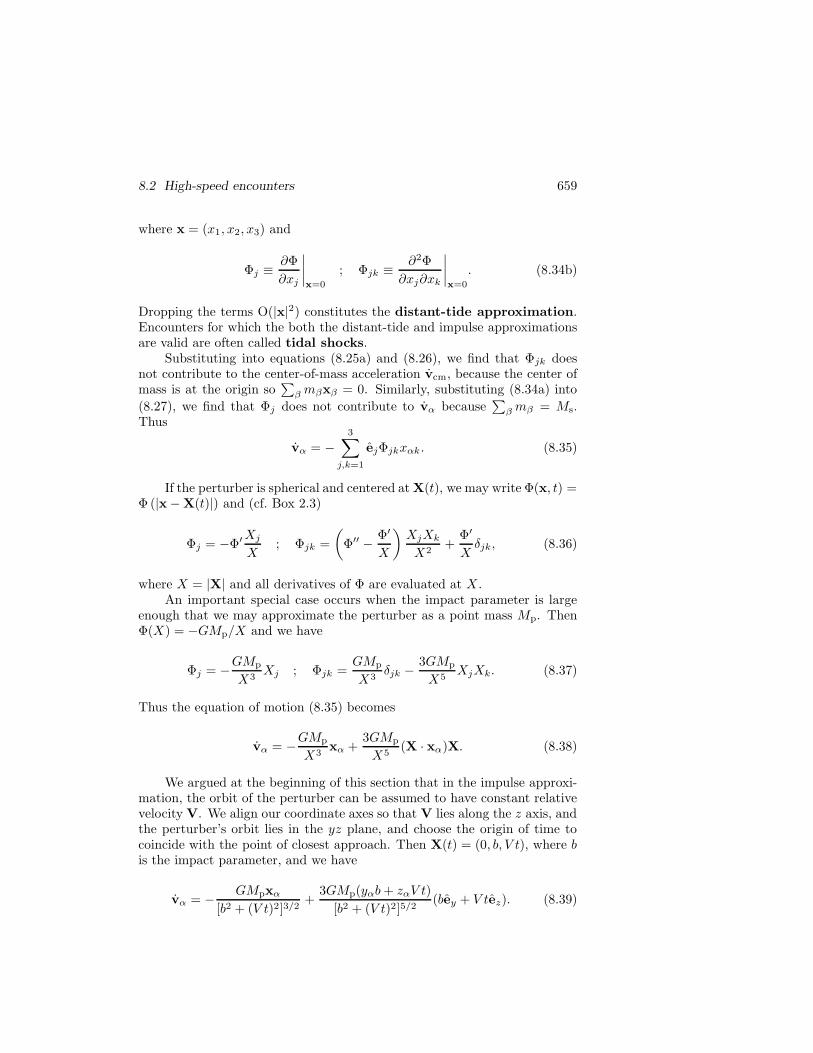
We argued at the beginning of this section that in the impulse approxi-mation, the orbit of the perturber can be assumed to have constant relativevelocity V. We align our coordinate axes so that V lies along the z axis, andthe perturber’s orbit lies in the yz plane, and choose the origin of time tocoincide with the point of closest approach. Then X(t) = (0, b, V t), where bis the impact parameter, and we have
v" = (GMpx"
[b2 + (V t)2]3/2+
3GMp(y"b + z"V t)
[b2 + (V t)2]5/2(bey + V tez). (8.39)

660 Chapter 8: Collisions and Encounters of Stellar Systems
In the impulse approximation, x" is constant during the encounter, so
"v" =
" #
"#dt v"
= GMp
" #
"#dt
0(
(x", y", z")
[b2 + (V t)2]3/2+ 3(0, b, V t)
y"b + z"V t
[b2 + (V t)2]5/2
1
=GMp
b2V
#( x"
" #
"#
du
(1 + u2)3/2, y"
" #
"#du
2 ( u2
(1 + u2)5/2,
z"
" #
"#du
2u2 ( 1
(1 + u2)5/2
$,
(8.40)where we have made the substitution u = V t/b. Evaluating the integrals inequation (8.40), we obtain finally
"v" =2GMp
b2V((x", y", 0). (8.41)
The error introduced in this formula by the distant-tide approximation is oforder |x|/b ' 1. The velocity increments tend to deform a sphere of starsinto an ellipsoid whose long axis lies in the direction of the perturber’s pointof closest approach. This distortion is reminiscent of the way in which theMoon raises tides on the surface of the oceans.
By equations (8.30) and (8.41) the change in the energy per unit massin the distant-tide approximation is (Spitzer 1958)
" 'E =2G2M2
p
V 2b4
+
"
m"(x2" + y2
"). (8.42)
If the subject system is spherical, then.
m"x2" =
.m"y2
" = 13Ms+r2,,
where +r2, is the mass-weighted mean-square radius of the stars in the subjectsystem. In this case equation (8.42) simplifies to
" 'E =4G2M2
pMs
3V 2b4+r2,. (8.43)
Equation (8.43) shows that for large impact parameter b the energy in-put in tidal shocks varies as b"4. Thus the encounters that have the strongeste!ect on a stellar system are those with the smallest impact parameter b,which unfortunately are also those for which the approximation of a point-mass perturber is invalid. Fortunately, it is a straightforward numericaltask to generalize these calculations to a spherical perturber with an arbi-trary mass distribution, using equations (8.30), (8.35), and (8.36) (Aguilar &White 1985; Gnedin, Hernquist, & Ostriker 1999). Let U(b/rh) be the ratio

8.2 High-speed encounters 661
Figure 8.4 Energy input in a tidalshock due to a perturber with aPlummer or Hernquist mass distribu-tion (eqs. 2.44b and 2.67). Here b isthe impact parameter, rh is the half-mass radius of the Plummer or Hern-quist model, and U is the ratio ofthe energy input to that caused by apoint mass perturber (eq. 8.44). Theintegral W =
Rdx U(x)/x3 = 0.5675
for the Plummer model and 1.239 forthe Hernquist model (eq. 8.52).
of the impulsive energy change caused by a perturber of half-mass radius rh
to the input from a point of the same total mass, which is given by (8.43).Then we have
" 'E =4G2M2
pMs
3V 2b4U(b/rh)+r2,. (8.44)
Figure 8.4 shows U(x) for the Plummer and Hernquist mass distributions.
8.2.2 Disruption of stellar systems by high-speed encounters
In many cases we are interested in the cumulative e!ect of encounters on astellar system that is traveling through a sea of perturbers. Let us assumethat the perturbers have mass Mp and number density np, and a Maxwelliandf with velocity dispersion #p in one dimension. Similarly, we assume thatthe subject system is a randomly chosen member of a population having aMaxwellian velocity distribution with dispersion #s.
Consider the rate at which the subject system encounters perturbersat relative speeds in the range (V, V + dV ) and impact parameters in therange (b, b + db). With our assumption of Maxwellian velocity distributions,the distribution of relative velocities of encounters is also Maxwellian, withdispersion (Problem 8.8)
#rel = (#2s + #2
p)1/2. (8.45)
Thus the probability that the subject system and perturber have relativespeed in the given range is
dP =4!V 2dV
(2!#2rel)
3/2exp
#(
V 2
2#2rel
$, (8.46)

662 Chapter 8: Collisions and Encounters of Stellar Systems
and the average rate at which a subject system encounters perturbers withspeed V and impact parameter b is
C = np V 2!b db dP =2)
2!npb db
#3rel
exp
#(
V 2
2#2rel
$V 3dV. (8.47)
In the distant-tide approximation, the energy input to a star is propor-tional to the square of its radius (eq. 8.42). So we focus on stars in the outerparts of the subject system, for which we can assume that the gravitationalpotential of the subject system is Keplerian. In a Keplerian potential, thetime averaged mean-square radius of an orbit with semi-major axis a andeccentricity e is (1 + 3
2e2)a2 (Problem 3.9). If the df of the subject sys-tem is isotropic in velocity space, the average of e2 over all the stars with agiven semi-major axis or energy is 1
2 (Problem 4.8). Thus, if we average overstars with di!erent orbital phases and eccentricities but the same energy,+r2, = 7
4a2, and equation (8.44) yields an average change in energy per unitmass of
+"E, =+" 'E,Ms
=7G2M2
pa2
3V 2b4U(b/rh). (8.48)
From Figure 8.4 we see that for b % rh, U ! 1 so +"E, $ b"4 is a steeplydeclining function of impact parameter. The frequency of encounters withimpact parameters in the range (b, b+db) is proportional to b db so the rate atwhich energy is injected by encounters in this range decreases with increasingb as db/b3. On the other hand, U rapidly decreases with decreasing b onceb &< rh, with the result that encounters with impact parameters b & rh inflictthe most damage.
If the damage from a single encounter with b & rh is not fatal for thesystem, we say that we are in the di"usive regime because the e!ects froma whole sequence of encounters will accumulate, as in the di!usive relaxationprocesses that we discussed in Chapter 7. If, by contrast, a single encounterat impact parameter b & rh will shatter the system, the damage sustained bythe system will be small until it is disrupted by a single, closest encounter,and we say that we are in the catastrophic regime.
(a) The catastrophic regime We first determine the largest impactparameter parameter b1 at which a single encounter can disrupt the system.Since we are in the catastrophic regime, we may assume that b1 &> rh sothe energy per unit mass injected by an encounter at impact parameter b1
is given by equation (8.48) with U(b/rh) ! 1. Equating this to the absolutevalue of the energy of an individual star E = (GMs/2a (eq. 3.32), we obtain
1 =+"E,|E|
=14GM2
pa3
3MsV 2b41
so b1(V ) = 1.5
#GM2
pa3
MsV 2
$1/4
. (8.49)

8.2 High-speed encounters 663
The rate at which disruptive encounters occur is then given by equation(8.47):
R *2)
2!np
#3rel
" #
0dV V 3 exp
#(
V 2
2#2rel
$ " b1(V )
0b db
=
*14
3!
G1/2npMpa3/2
M1/2s
.
(8.50)
The disruption time of a subject system with semi-major axis a is
td ! R"1 ! kcat1
G$p
#GMs
a3
$1/2
, (8.51)
where $p * Mpnp is the mass density of perturbers and kcat is of order unity.Our analytic treatment yields kcat = 0.15 but Monte-Carlo simulations ofcatastrophic disruption suggest that kcat ! 0.07 (Bahcall, Hut, & Tremaine1985). It is remarkable that the disruption time in the catastrophic regimeis independent of both the velocity dispersion #rel and the mass of individualperturbers, so long as their overall mass density $p is fixed.
(b) The di"usive regime In this regime, each encounter imparts a ve-locity impulse "v (eq. 8.28) that satisfies |"v| ' |v|. The correspondingchange in the energy per unit mass is "E = v ·"v + 1
2 |"v|2. Thus the dif-fusion term v ·"v is much larger than the heating term 1
2 |"v|2. On theother hand the direction of the velocity impulse, which depends on the rel-ative orientation of the star and the perturber, is usually uncorrelated withthe direction of the velocity v of the star relative to the center of mass of thesubject system, which depends on the orbital phase of the star. Thus theaverage of the di!usion term over many encounters is zero, while the heat-ing term systematically increases the energy.7 An accurate description of theevolution of the energy under the influence of many high-speed encountersrequires the inclusion of both terms, using the Fokker–Planck equation thatwe described in §7.4.2. Nevertheless, for the sake of simplicity, and since ourestimates will be crude anyway, we focus our attention exclusively on theheating term.
Combining equations (8.47) and (8.48), we find that the rate of energyincrease for stars with semi-major axis a is
E = C +"E,
=14
3
)2!
G2M2pnpa2
#3rel
" #
0dV V exp
#(
V 2
2#2rel
$ "db
b3U(b/rh)
=14
3
)2!
G2M2pnpa2
#relr2h
W, where W *"
dx
x3U(x).
(8.52)
7 This argument is similar to, but distinct from, the argument leading from equa-tion (8.29) to equation (8.30), which involved an average over the e"ects of a single col-lision on many stars rather than an average over the e"ect of many collisions on a singlestar.

664 Chapter 8: Collisions and Encounters of Stellar Systems
In general, W must be evaluated numerically for a given mass model. Fora Plummer model, W = 0.5675 and for a Hernquist model W = 1.239(Figure 8.4).
For point-mass perturbers, U(x) = 1, and the heating rate is
E =14
3
)2!
G2M2pnpa2
#rel
"db
b3. (8.53)
This integral over impact parameter diverges at small b. In practice, thedistant-tide approximation fails when the impact parameter is comparableto the size of the subject system, so the integration should be cut o! at thispoint.
Comparing the heating rate (8.52) to the energy of an individual starE = ( 1
2GMs/a, we obtain the time required for the star to escape:
td !|E|E
!0.043
W
#relMsr2h
GM2pnpa3
. (8.54)
For point-mass perturbers, we use equation (8.53), with the integration overimpact parameter cut o! at bmin:
td !|E|E
! 0.085#relMsb2
min
GM2pnpa3
. (8.55)
These are only approximate estimates. A more accurate treatment wouldemploy the Fokker–Planck equation (7.123); in this equation the di!usioncoe#cient D["E] is the quantity here called E, and the di!usion coe#cientD[("E)2] would be computed similarly as the rate of change of the mean-square energy. Generally this treatment gives a half-life for a star with agiven semi-major axis that is a few times shorter than the estimate (8.54).
(c) Disruption of open clusters The masses of open clusters lie in therange 102 M! &< Mc &< 104 M!, and their half-mass radii and internal veloc-ity dispersions are rh,c " 2 pc and #c " 0.3 km s"1 (Table 1.3). The crossingtime at the half-mass radius is rh,c/#c " 10 Myr. Much of the interstellargas in our Galaxy is concentrated into a few thousand giant molecularclouds of mass Mgmc &> 105 M! and radius rh,gmc " 10 pc. Both openclusters and molecular clouds travel on nearly circular orbits through theGalactic disk, with random velocities of order 7 km s"1; thus the dispersionin relative velocity is #rel !
)2 # 7 km s"1 ! 10 km s"1 (eq. 8.45). The du-
ration of a cluster-cloud encounter with impact parameter b > rgmc is thenb/#rel ! (b/10 pc)Myr, which is shorter than the cluster crossing time forb &< 100 pc. Thus we may use the impulse approximation to study the e!ectof close encounters with molecular clouds on open clusters.
The impact parameter at which a typical encounter with a point-massperturber would disrupt the cluster is given by equation (8.49); identifying

8.2 High-speed encounters 665
Figure 8.5 The fraction ofnearby open clusters youngerthan a given age. The clustersample is from Piskunov et al.(2007). The curve is derivedfrom a simple theoretical modelin which clusters are born ata constant rate and the prob-ability that a cluster survivesfor time t is exp("t/") with" ! 300 Myr. A Kolmogorov–Smirnov test (Press et al. 1986)shows that the two distribu-tions are statistically indistin-guishable.
the open cluster with the subject system and the molecular cloud with theperturber we obtain
b1(#rel) = 15 pc
#Mgmc
105 M!
$1/2 #300M!
Mc
$1/4
##
a
2 pc
$3/4 #10 km s"1
#rel
$1/2
.
(8.56)
Since this distance is larger than the cloud size rh,gmc " 10 pc, even whenthe semi-major axis is as small as the typical cluster half-mass radius of 2 pc,the encounters are in the catastrophic regime. Hence the disruption time isgiven by equation (8.51):
td ! 250 Myrkcat
0.07
0.025M! pc"3
$gmc
#Mc
300M!
$1/2 #2 pc
a
$3/2
, (8.57)
where the mean density of gas in molecular clouds is taken to be about halfof the total gas density in the solar neighborhood (see Table 1.1).
This result is quite uncertain, not only because the derivation of equa-tion (8.57) is highly idealized, but also because of uncertainties in the molec-ular cloud parameters and the large dispersion in open-cluster parameters.Nevertheless, the available data suggest that the median lifetime of openclusters is remarkably close to this simple estimate (Figure 8.5). In fact, itwas the observation that there are few open clusters with ages &> 500 Myrthat prompted Spitzer (1958) to argue that clusters might be dissolved bythe very clouds that bring them into the world.
(d) Disruption of binary stars Binary stars can be thought of as clus-ters with just two members and, like clusters, they can be disrupted by

666 Chapter 8: Collisions and Encounters of Stellar Systems
encounters with passing perturbers. Obviously the vulnerability of a binaryto disruption is an increasing function of the semi-major axis a of its com-ponents. Binary semi-major axes are usually measured in terms of the as-tronomical unit, 1 AU = 1.496# 1011 m = 4.848# 10"6 pc (approximatelythe mean Earth-Sun distance; see Appendix A).
First we consider disruption of binaries in the solar neighborhood bypassing stars. We focus on stars—both the binary components and theirperturbers—that have ages comparable to the age of the Galaxy and massescomparable to that of the Sun, since these contain most of the stellar massin the solar neighborhood. The velocity distribution of such stars is triaxial,but we may approximate this distribution by an isotropic Maxwellian with aone-dimensional dispersion #! ! 30 km s"1 (1/
)3 of the rms velocity, from
Table 1.2). The velocity distribution is the same for single and binary stars,so the relative dispersion is #rel =
)2 # 30 km s"1 ! 40 km s"1 (eq. 8.45).
According to equation (8.49), the maximum impact parameter for acatastrophic encounter between a binary star of total mass Mb and a passingstar of mass Mp is
b1(#rel) ! 1.5a
2GM2
p
Mb#2rela
31/4
! 0.11a
#2M!
Mb
104 AU
a
$1/4 #Mp
1M!
40 km s"1
#rel
$1/2
.
(8.58)
Unless the semi-major axis is so small that the probability of a close en-counter is negligible, this result shows that b1 &< a for solar-type stars in thesolar neighborhood, and thus that the encounters are in the di!usive regime.The disruption time is given by equation (8.55), setting bmin & a, where thedistant-tide approximation fails; thus (Opik 1932; Heggie 1975)
td ! kdi!#relMb
GM2pnpa
, (8.59)
where kdi! * 0.085(bmin/a)2. We can refine this estimate by recalling thediscussion of the disruption of soft binaries in §7.5.7a; equation (7.173) inthat section describes the disruption time in the di!usive regime for thecase in which the component stars of the binary have the same mass asthe perturbing stars, so Mb = 2Mp, and the velocity dispersion # of theperturbers and the binaries is the same, so #rel =
)2#. Equating the two
expressions, we find kdi! ! 0.022/ ln%, where % " #2rela/(GMp). For binaries
with a & 104 AU in the solar neighborhood, this formula yields kdi! ! 0.002,and Monte Carlo simulations yield a similar value (Bahcall, Hut, & Tremaine1985). The rather small value of kdi! arises in part because E grows asa2, so the heating rate accelerates as the binary gains energy, and in part

8.2 High-speed encounters 667
because close encounters with either member of the binary contribute to thedisruption rate, an e!ect not accounted for in equation (8.53).
In the solar neighborhood, equation (8.59) yields
td ! 15 Gyrkdi!
0.002
#rel
40 km s"1
Mb
2M!
#1M!
Mp
$2 0.05 pc"3
np
104 AU
a. (8.60)
Thus the upper limit to the semi-major axes of old binary stars in the solarneighborhood is a ! 2 # 104 AU.
Now consider the e!ects of molecular clouds. Replacing the perturbermass Mp in equation (8.58) by the typical cloud mass Mgmc " 105 M!, wefind that the maximum impact parameter for impulsive disruption is
b1(#rel) ! 1.9 pc
#2M!
Mb
$1/4 ( a
104 AU
)3/4#
Mgmc
105 M!
30 km s"1
#rel
$1/2
.
(8.61)We have used a fiducial value #rel = 30 km s"1, which is the sum in quadra-ture of the dispersions of the stars, #! ! 30 km s"1, and the clouds, #gmc !7 km s"1. Since b1 is smaller than the cloud radius rh,gmc " 10 pc, the en-counters are in the di!usive regime. The disruption time can be estimatedfrom equation (8.54), using the value W = 0.5675 appropriate for a Plummermodel of the cloud’s density distribution:
td ! 0.075#relMbr2
h,gmc
GM2gmcngmca3
. (8.62)
The cloud parameters Mgmc, ngmc, and rh,gmc are all poorly known. For-tunately, they enter this equation in terms of the observationally accessiblecombinations $gmc * (M/!r2
h)gmc, the mean surface density of a cloud,and $gmc = (Mn)gmc, the mean density of molecular gas. We adopt$gmc ! 300M! pc"2 and $gmc ! 0.025M! pc"3 (Hut & Tremaine 1985).Thus
td ! 380 GyrMb
2M!
#104 AU
a
$3#rel
30 km s"1. (8.63)
Although this result is subject to substantial uncertainties, together withequation (8.60) it implies that binaries with semi-major axes &> 2#104 AU !0.1 pc cannot survive in the solar neighborhood for its lifetime of & 10 Gyr,due to the combined e!ects of high-speed encounters with molecular cloudsand other stars.
The widest known binary stars in the disk do indeed have separationsof about 0.1 pc (Chaname & Gould 2004); however, there is little evidencefor or against the cuto! in the binary distribution that we have predicted atthis separation (Wasserman & Weinberg 1987). Binary stars in the stellarhalo appear to exist with even larger separations; such binaries can survive

668 Chapter 8: Collisions and Encounters of Stellar Systems
because their velocity #rel relative to the disk is much higher, and becausethey spend only a fraction of their orbit in the disk, so the disruptive e!ectsfrom disk stars and molecular clouds are much weaker (Yoo, Chaname, &Gould 2004).
(e) Dynamical constraints on MACHOs One possible constituentof the dark halo is machos, compact objects such as black holes or non-luminous stars (§1.1.2). Suppose that machos contribute a fraction fh &> 0.5of the radial force in the solar neighborhood; this is close to the maximumallowed since the disk contributes a fraction fd = 1(fh &> 0.4 (§6.3.3). Thenlimits on the optical depth of the dark halo to gravitational lensing (Alcocket al. 2001; Tisserand et al. 2007) imply that the macho mass
m &< 10"7 M! or m &> 30M!. (8.64)
In §7.4.4 we showed that encounters between machos and disk stars addkinetic energy to the disk stars and thereby increase both the velocity dis-persion and the disk thickness; even if this is the only mechanism that heatsthe disk—and we shall see in §8.4 that it is not—the observed dispersionrequires that m &< 5–10 # 106 M! (eq. 7.104). We now investigate whatadditional constraints can be placed on the macho mass by the e!ect ofhigh-speed encounters of machos on binary stars.
We write the number density of machos as n = $/m. If the macho
mass is small enough, disruption is in the di!usive regime, and we can useequation (8.59) to estimate the disruption time:
td,di! ! kdi!#relMb
Gm$a(kdi! " 0.002), (8.65a)
where Mb is the mass of the binary. In the catastrophic regime, the disrup-tion time is given by equation (8.51):
td,cat ! kcatM1/2
b
G1/2$a3/2(kcat " 0.07). (8.65b)
The transition between these two regimes occurs when the critical impactparameter b1(#rel) (eq. 8.49) is of order the binary semi-major axis a; how-ever, a more accurate way to determine the transition is to set the actualdisruption time to
td = min (td,di! , td,cat) (8.66)
and identify the transition with the macho mass mcrit at which td,di! =td,cat. Thus we find
mcrit =kdi!
kcat
##2
relMba
G
$1/2
(kdi!kcat " 0.03). (8.67)

8.2 High-speed encounters 669
Notice that for m > mcrit, the disruption time td,cat depends on the overalldensity contributed by the machos but not their individual masses. Thus thesurvival of a given type of binary system either rules out all macho massesabove mcrit and some masses below mcrit (if the system’s age exceeds td,cat)or does not rule out any masses (if its age is less than td,cat).
To plug in numbers for the solar neighborhood, we use the simple modelfor the df of machos in the dark halo that we described on page 584. Inthis model the local density of machos is given by equation (7.94), and therelative dispersion between machos is #rel =
)2# = vc, where vc is the
circular speed (eq. 8.45)—this is also roughly the dispersion between themachos and stars, whether they belong to the disk or the stellar halo. Then
mcrit ! 30M!kdi!/kcat
0.03
#Mb
2M!
a
104 AU
$1/2 vc
220 km s"1. (8.68)
To evaluate the disruption time in the catastrophic regime, m > mcrit, weuse equation (8.65b), and take the local macho density from equation (7.94).Assuming the solar radius R0 = 8 kpc and the solar circular speed vc = v0 =220 km s"1, we have
td,cat ! 20 Gyr0.5
fh
kcat
0.07
#104 AU
a
$3/2
. (8.69)
For dark-halo fractions fh ! 0.5, the disruption time td,cat is larger than10 Gyr for semi-major axes a &< 1.6 # 104 AU. In the di!usive regime, thedisruption time is even longer. Disk binaries with semi-major axes largerthan this limit are likely to be disrupted by encounters with other disk stars(eq. 8.59) and so we cannot probe the macho mass with disk binaries. Halobinaries are much less susceptible to other stars and molecular clouds, be-cause they spend only a small fraction of their time in the disk, and thereforemight be present with semi-major axes large enough to provide useful con-straints on the macho population. Thus, if a population of halo binaries witha &> 2 # 104 AU were discovered, we could rule out a substantial contribu-tion to the local gravitational field for all macho masses exceeding 30M!(eq. 8.68). Yoo, Chaname, & Gould (2004) o!er evidence that halo bina-ries exist with semi-major axes as large as a & 105 AU. Together with themicrolensing constraint (8.64) this conclusion, if verified by larger samples,would virtually rule out machos as a significant constituent of the dark haloin the solar neighborhood.
(f) Disk and bulge shocks Globular clusters in disk galaxies passthrough the disk plane twice per orbit. As they cross the plane, the gravita-tional field of the disk exerts a compressive gravitational force which is su-perposed on the cluster’s own gravitational field, pinching the cluster brieflyalong the normal to the disk plane. Repeated pinching at successive passages

670 Chapter 8: Collisions and Encounters of Stellar Systems
through the disk can eventually disrupt the cluster. This process is knownas disk shocking (Ostriker, Spitzer, & Chevalier 1972).
Let Z * Zcm +z be the height above the disk midplane of a cluster star,with Zcm(t) the height of the cluster’s center of mass. Then so long as thecluster is small compared to the disk thickness, we may use the distant-tideapproximation, and equation (8.35) yields
vz = (#
'2&d
'Z2
$
cm
z, (8.70)
where vz = z is the z-velocity of the star relative to the cluster center.The gravitational potential arising from a thin disk of density $d(R, z)
is &d(R, Z), where (eq. 2.74)
d2&d
dZ2= 4!G$d. (8.71)
Thusvz = (4!G$d(R, Zcm)z, (8.72)
where R is the radius at which the cluster crosses the disk.If the passage of the cluster through the disk is su#ciently fast for the
impulse approximation to hold, z is constant during this passage, and thevelocity impulse is
"vz =
"dt vz = (4!Gz
"dt $d[R, Zcm(t)]. (8.73)
To a good approximation we can assume that the velocity of the center ofmass of the cluster is constant as it flies through the disk, so Zcm(t) =Vzt + constant , where Vz is the Z-velocity of the cluster; eliminating thedummy variable t in favor of Zcm we have
"vz = (4!Gz
|Vz |
"dZcm $d(R, Zcm) = (
4!G$d(R)z
|Vz |, (8.74)
where $d(R) *!
dZ$d(R, Z) is the surface density of the disk.From equation (8.30), the energy per unit mass gained by the cluster in
a single disk passage is
"E = 12 +("vz)2, =
8!2G2$2d
V 2z
+z2,. (8.75)
If the cluster is spherically symmetric, the average value of z2 for stars at agiven radius r is 1
3r2. As shown on page 662, if the cluster has an ergodic df

8.2 High-speed encounters 671
the average value of r2 for stars with a given semi-major axis is 74a2. Thus
the energy gain is
"E =14!2G2$2
da2
3V 2z
. (8.76)
The cluster passes through the disk twice in each orbital period T$, so thedisruption time is
td ! 12T$
|E|"E
= 0.005MgcV 2
z T$
G$2da3
, (8.77)
where we have set E = 12GMgc/a, since the potential is Keplerian in the
outer parts of the cluster, where the e!ect of disk shocking is strongest.8
In the solar neighborhood the Galactic disk has a midplane volume den-sity $ ! 0.10M! pc"3, and surface density $d ! 50M! pc"2 (Table 1.1).The e!ective thickness of the disk is h * $d/$ ! 500 pc. If we approximatethe potential of the Milky Way as spherically symmetric, with circular speedvc at all radii, then the mean-square speed of a collection of test particlessuch as clusters is +V 2, = v2
c (Problem 4.35), so if the cluster distributionis spherical, we expect that +V 2
z , = 13v2
c ; thus +V 2z ,1/2 ! 130 km s"1 for
vc ! 220 km s"1. Equation (8.77) can be rewritten
td ! 340 GyrMgc
2 # 105 M!
T$
200 Myr
##
Vz
130 km s"1
$2 #50M! pc"2
$d
$2 #10 pc
a
$3
.
(8.78)
This result is based on the impulse approximation, whose validity we mustcheck. The duration of the encounter of the cluster with the disk is % "h/Vz ! 4 Myr for Vz ! 130 km s"1 and h ! 500 pc. The crossing time inthe outer parts of the cluster is roughly the inverse of the orbital frequency,(a3/GMgc)1/2 ! 1 Myr (a/10 pc)3/2 for a cluster mass of 2 # 105 M!. Thusthe impulse approximation is valid only in the outer parts of the cluster,a &> 30 pc, and at these semi-major axes the disruption time is &< 10 Gyr. Weconclude that disk shocks can lead to substantial erosion of the outermoststars in a typical globular cluster orbiting at the solar radius. For clustersorbiting at smaller radii, disk shocks are even more important, since theorbital time is shorter and the disk surface density is larger.
Bulge shocking is a closely related process. Here the rapidly changingexternal gravitational field arises as a cluster on a highly eccentric orbit
8 A subtle but important assumption in deriving this result is that the orbital phaseand thus the value of the height z is uncorrelated between successive disk passages. Thisassumption is plausible because the interval between successive disk passages is likely tovary considerably for an eccentric, inclined cluster orbit in a realistic disk galaxy potential.

672 Chapter 8: Collisions and Encounters of Stellar Systems
plunges through the bulge of a disk galaxy or the dense center of an ellipticalgalaxy. In this case the use of the term “shock” is less apt, since the durationof the encounter is not very short compared to the crossing time, even in theouter parts of the cluster, and the impulse approximation is not strictlyvalid. Nevertheless, the results are similar: the encounters systematicallypump energy into the stars in the outer cluster, leading to the escape ofstars and the eventual dissolution of the cluster.
The evolution of the globular-cluster population under the influence ofdisk and bulge shocks is described in §7.5.6.
(g) High-speed interactions in clusters of galaxies The study ofgalaxies in clusters provides unique insights into galaxy formation and evo-lution, not only because many dynamical processes are stronger and moreobvious in the high-density cluster environment, but also because clusters canbe detected at high redshift, enabling the evolution of the galaxy populationto be studied directly.
The relative velocities between galaxies in a rich cluster, & 2000 km s"1,are so large that collisions of galaxies last only a few Myr, far less than thecrossing time in the galaxy, so they can be treated by the impulse approxi-mation. We model the cluster as a singular isothermal sphere, with density$(r) = #2/(2!Gr2) (eq. 4.103). In clusters the galaxies and dark matter havea similar distribution, so it is reasonable to assume that the ratio M! * $/nof the mass density to the galaxy number density—in other words the massper galaxy—is constant. (Note that this is not necessarily the mass of thegalaxy, since most of the mass is probably spread uniformly through thecluster and is not associated with any individual galaxies.) We focus ongalaxies with the characteristic luminosity L! = 2.9#1010 L! in the R band(eq. 1.18). The mass-to-light ratio in rich clusters is (R " 200(! (eq. 1.25)so the mass associated with each L! galaxy is
M! = (RL! " 6 # 1012 M!. (8.79)
Consequently, the number density of L! galaxies is
n(r) =$(r)
M!=
#2
2!GM!r2. (8.80)
Now let us estimate the rate at which a given galaxy encounters othergalaxies. The velocity dispersion in clusters is so high that gravitationalfocusing is negligible, so if galaxies are deemed to collide when their centerscome within a collision radius rcoll, then from equation (7.194) the collisiontime is given by
1
tcoll= 4
)!n#r2
coll !2)!
#3r2coll
GM!r2. (8.81)

8.2 High-speed encounters 673
After replacing rcoll with 2rh, where rh is the galaxy radius, equation (8.81)yields
tcoll ! 0.2GM!r2
#3r2h
! 6 Gyr
#800 km s"1
#
$3 #20 kpc
rh
r
0.5 Mpc
$2 M!
5 # 1012 M!.
(8.82)Thus the stellar component of a galaxy in the central 0.5 Mpc of a rich clusteris likely to have su!ered at least one close encounter with another galaxy.What are the consequences of such encounters?
As we have seen, high-speed collisions between galaxies have only asmall e!ect on the distribution of stars, but if both galaxies contain gas disksthe gas will su!er a violent collision and be lost from the galaxies. Spitzer& Baade (1951) suggested that collisions might transform spiral galaxiesinto gas-free lenticular galaxies, thereby explaining the observation that spi-rals are replaced by lenticulars in high-density environments such as clusters(§1.1.3). An alternative and more likely explanation (Gunn & Gott 1972) isthat ram pressure, heating, and other interactions with hot intergalactic gasin the cluster have gradually eroded the gas disks of spiral galaxies (see vanGorkom 2004 for a review).
Isolated galaxies have dark halos that extend to several hundred kpc. Inclusters, encounters strip o! the outer parts of these halos, so we expect thatcluster galaxies will have much smaller and less massive halos than galaxiesin low-density environments. We can make a crude estimate of this e!ectusing equation (8.54). For this purpose, we assume that the subject systemand the perturber are identical. Thus Ms = Mp = M and #rel =
)2#
where # is the velocity dispersion in the cluster. We set the dimensionlessparameter W " 1, and set rh = a to estimate the disruption time for starsat the half-mass radius. Thus
td ! 0.06#
GMnrh. (8.83)
We eliminate the number density n using equation (8.80), and write the massM of the galaxy in terms of rh and its velocity dispersion #2
s = 13 +v
2,, usingthe virial theorem in the form (4.249b); the dispersion for an L! galaxy is#s ! 200 km s"1 (eq. 1.21). Thus
td ! 0.056GM!r2
##2s r2
h
! 3.8 GyrM!
5 # 1012 M!
800 km s"1
#
#200 km s"1
#s
$2 #r
0.5 Mpc
50 kpc
rh
$2
.
(8.84)Note that the disruption time is related to the collision time (eq. 8.82) bythe simple formula td/tcoll ! 0.25(#/#s)2; as the velocity dispersion # of the

674 Chapter 8: Collisions and Encounters of Stellar Systems
cluster increases relative to the dispersion #s of the galaxies, gravitationalinteractions become less and less important relative to physical collisions.
This result shows that encounters with other galaxies will erode thedark halos of galaxies residing in the inner 0.5 Mpc of a rich cluster to aradius rh &< 50 kpc. Most of the dark-halo mass has therefore been strippedfrom the individual galaxies, and is now smoothly distributed throughout thecluster (Richstone 1976). Since the disruption time is proportional to Ms/a3
(eq. 8.54) and thus to the mean density of the subject system, low-densitygalaxies are more severely a!ected by encounters, and can be completelydisrupted near the cluster center. The large-scale static tidal field of thecluster also strips the outer halo of cluster galaxies, a process that we shallinvestigate in the next section.
Clusters form hierarchically from smaller systems that resemble groupsof galaxies (§§1.1.5 and 9.2.2). Groups have velocity dispersions of only &300 km s"1, so encounters in groups occur at lower speeds and have strongere!ects—they frequently lead to mergers—and dynamical friction is morepowerful. Most of the galaxy evolution that we see in the centers of richclusters may thus be due to “pre-processing” in the groups that later mergedto form the cluster. For example, the exceptionally luminous brightest clustergalaxies or cD galaxies (§1.1.3) that are found at the centers of clustersprobably arise from the merger of galaxies in precursor groups (Dubinski1998).
8.3 Tides
In the last section we examined how tidal shocks from high-speed encountersheat stellar systems and erode their outer parts. We now consider the oppo-site limiting case of a static tidal field. The simplest example of a static tideoccurs when a satellite travels on a circular orbit in the gravitational field ofa much larger spherical host system. In this case, the satellite experiencesno shocks—in fact, in the frame rotating with the satellite the external tidalfield is stationary—so in the absence of other relaxation e!ects, a su#cientlysmall system could survive indefinitely. However, a static tidal field prunesdistant stars from the satellite system, thereby enforcing an upper limit onits size. Observationally, globular clusters and other satellite systems oftenshow a fairly sharp outer boundary, which is called the tidal radius on theassumption that it is caused by this process (see §4.3.3c, BM §6.1.10, andKing 1962).
In the following subsections, we analyze the e!ect of a tidal field on asatellite in a circular orbit using two complementary approaches.

8.3 Tides 675
8.3.1 The restricted three-body problem
Let us suppose that the host and satellite systems are point masses M andm, traveling at separation R0 in a circular orbit around their mutual centerof mass. The restricted three-body problem is to find the trajectoryof a massless test particle that orbits in the combined gravitational field ofthese two masses (Szebehely 1967; Henon 1997; Valtonen & Karttunen 2006).Solutions of this problem provide a good approximation to the motion of starsin the outer parts of a satellite stellar system that is on a circular orbit nearor beyond the outer edge of a spherical host system.
The two masses orbit their common center of mass with angular speed
' =
4G(M + m)
R30
, (8.85)
so the gravitational field is stationary when referred to a coordinate systemcentered on the center of mass that rotates at speed '. We orient thiscoordinate system so that the centers of the satellite and host systems areat xm = [MR0/(M + m), 0, 0] and xM = [(mR0/(M + m), 0, 0], and theangular speed is ! = (0, 0, '). In §3.3.2 we showed that on any orbit in sucha system, the Jacobi integral
EJ = 12v2 + &(x) ( 1
2 |!# x|2
= 12v2 + &e!(x)
(8.86)
is conserved (eq. 3.113). Since v2 - 0, a star with Jacobi integral EJ cannever trespass into a region where &e!(x) > EJ. Consequently, the surface&e!(x) = EJ, the zero-velocity surface for stars of Jacobi integral EJ, formsan impenetrable wall for such stars. Figure 8.6 shows contours of constant&e! in the equatorial plane of two orbiting point masses; the Lagrange pointsare the extrema (maxima and saddle points) of this surface. It is instructiveto compare these contours to those in a bar-like potential, shown in Fig-ure 3.14.9 The stability of orbits near the Lagrange points in the restrictedthree-body problem is discussed in Problem 3.25.
From the figure we see that the zero-velocity surfaces near each bodyare centered on it, but farther out the zero-velocity surfaces surround bothbodies. Hence, at the critical value of &e! corresponding to the last zero-velocity surface to enclose only one body, there is a discontinuous changein the region confined by the Jacobi integral. The last closed zero-velocitysurface surrounding a single body is called its tidal or Roche surface; sincethis surface touches the Lagrange point L3 that lies between the two masses
9 Note that di"erent authors use di"erent conventions for the numbering of the La-grange points L1, L2, L3.

676 Chapter 8: Collisions and Encounters of Stellar Systems
Figure 8.6 Contours of equal e"ective potential #e! defined by equation (8.88) for twopoint masses in a circular orbit. The mass ratio m/M = 1
9 . The points L1, . . . , L5 are theLagrange points. The L4 and L5 points form an equilateral triangle with the two masses(Problem 3.25).
on the line connecting them, it is natural to identify the tidal radius of m asthe distance rJ between m and L3.
We may evaluate rJ by noticing that at (xm ( rJ, 0, 0) the e!ectivepotential has a saddle point, so
#'&e!
'x
$
(xm"rJ,0,0)
= 0. (8.87)
For two point masses a distance R0 apart, equations (8.85) and (8.86) imply
&e!(x) = (G
%M
|x ( xM |+
m
|x ( xm|+
M + m
2R30
(x2 + y2)
&. (8.88)
At a point between the two masses, (8.87) is satisfied if
0 =1
G
#'&e!
'x
$
(xm"rJ,0,0)
=M
(R0 ( rJ)2(
m
r2J
(M + m
R30
#MR0
M + m( rJ
$.
(8.89)

8.3 Tides 677
This equation leads to a fifth-order polynomial whose roots give rJ. In gen-eral these roots must be found numerically. However, if the satellite is small,m ' M , then rJ ' R0, and we can expand (R0 ( rJ)"2 in powers of rJ/R0
to find
0 =M
R20
#1 +
2rJ
R0+ · · ·
$(
m
r2J
(M
R20
+M + m
R30
rJ !3MrJ
R30
(m
r2J
. (8.90)
Truncating the series in this way is none other than the distant-tide approx-imation. Then to first order in rJ/R0,
rJ =( m
3M
)1/3R0. (8.91)
We call the radius rJ the Jacobi radius of the mass m; alternativenames are the Roche or Hill radius. The Jacobi radius of an orbitingstellar system is expected to correspond to the observational tidal radius,the maximum extent of the satellite system. However this correspondence isonly approximate, for several reasons:(i) The tidal surface is not spherical (see Problem 8.12), so it cannot be
fully characterized by a single radius.(ii) All we have established is that a test particle can never cross the tidal
surface if it lies inside the tidal surface and has a velocity (in the rotat-ing frame) small enough that EJ < &e!(L3). Stars with larger velocitiesmay or may not escape from the satellite; conversely, stars that lie out-side the tidal surface can, in some cases, remain close to the satellite forall future times (see Problem 8.14 and Henon 1970). The approximatecorrespondence between the Jacobi radius and the observational tidalradius arises because the fraction of velocity space occupied by orbitsthat remain close to the satellite diminishes rapidly beyond rJ.
(iii) In most applications, the satellite system is not on a circular orbit.When m is on an eccentric orbit, there is no reference frame in whichthe potential experienced by a test particle is stationary, and no ana-log of the Jacobi integral exists.10 Thus no direct generalization of ourderivation of the Jacobi radius to the case of non-circular satellite orbitsis possible. King (1962) and others have argued that if the satellite is ona non-circular orbit, the tidal radius is still given by equation (8.91), butwith R0 replaced by the pericenter distance (we used an analogous ar-gument to describe the tidal disruption of stars orbiting a massive blackhole; see eq. 7.200). A more accurate approach is to recognize that thee!ect of tidal fields on satellites in non-circular orbits is intermediatebetween tidal radii—a concept that applies to circular orbits—and tidalshocks—which apply to high-velocity or plunging orbits. The tidal ra-dius limits the satellite at a fixed size, no matter how many orbits it
10 Although analogs of the Lagrange points can exist (Szebehely 1967).

678 Chapter 8: Collisions and Encounters of Stellar Systems
Figure 8.7 The rotating (x, y) coordinate systemused in Hill’s approximation.
travels, while tidal shocks prune the satellite more and more at everypericenter passage.
(iv) Stars are usually lost from the satellite as a result of weak perturbations,such as two-body relaxation, that drive EJ slightly higher than &e!(L3).Such stars drift slowly away from the satellite and thus can remain closeto the satellite for many orbital periods, thereby contributing to the starcounts even though they are no longer bound to the satellite (Fukushige& Heggie 2000).
(v) In many cases, the satellite orbits within the body of the host system,so the point-mass approximation used in deriving equation (8.91) is notaccurate. This defect, at least, is easy to remedy—see equation (8.106)below.
Tidal forces can be thought of as imposing a limit on the density of a satellite.Let $ * m/( 4
3!r3J) be the mean density of the satellite within a distance rJ,
and $h * M/(43!R3
0) be the mean density of the host inside the orbital radiusR0. Then equation (8.91) states that
$ = 3$h; (8.92)
to within a factor of order unity, a satellite is pruned by tidal forces untilits mean density equals the mean density of its host interior to its orbitalradius.
8.3.2 The sheared-sheet or Hill’s approximation
When the satellite is much smaller than the distance to the center of the hostsystem, we can use the distant-tide approximation for the host’s gravitationalfield (§8.2.1). We consider a spherically symmetric host system with potential&(R) at a distance R from its center; here we do not assume that the hostis a point mass, so &(R) is not necessarily the Keplerian potential (GM/R.We assume that the satellite travels on a circular orbit at distance R0 fromthe center of the host. We work in a frame with origin at the center of mass

8.3 Tides 679
of the satellite, in which the x-y plane coincides with the orbital plane of thesatellite, ex points directly away from the center of the host system, and ey
points in the direction of the orbital motion of the satellite (see Figure 8.7).This frame rotates with the circular frequency!0 * '0ez, so the accelerationof a particle in the satellite is given by equation (3.116),
d2x
dt2= (!& ( 2!0 #
dx
dt(!0 # (!0 # x), (8.93)
where
!& = !&s +3+
k=1
&jkxk. (8.94)
Here &s(x) is the gravitational potential from the satellite, and the secondterm arises from the distant-tide approximation (8.35). In our coordinatesystem, the center of the host is located at X = ((R0, 0, 0) and from equa-tion (8.36):
&xx = &%%(R0) ; &yy = &zz =&%(R0)
R0; &xy = &xz = &yz = 0.
(8.95)The equations of motion (8.93) read
x = 2'0y +,'2
0 ( &%%(R0)-x (
'&s
'x;
y = (2'0x +
%'2
0 (&%(R0)
R0
&y (
'&s
'y;
z = (&%(R0)
R0z (
'&s
'z.
(8.96)
Using the relation &%(R0) = R0'20 we see that the term in square brack-
ets in the second line vanishes. Moreover we can rewrite '20 ( &%%(R0) as
(2R0'0'%(R0) and this in turn can be rewritten as 4'0A0 where A0 =A(R0) is given by equation (3.83). Thus
x(2'0y(4'0A0x = ('&s
'x; y+2'0x = (
'&s
'y; z+'2
0z = ('&s
'z. (8.97)
These are the equations of motion in the sheared sheet or Hill’s approxi-mation, named after the mathematician G. W. Hill, who used this approachto study the motion of the Moon in the nineteenth century (Murray & Der-mott 1999).
(a) The epicycle approximation and Hill’s approximation We firstconsider the trajectories of test particles in the absence of a satellite, &s(x) =0. The simplest solutions of equations (8.97) have the form
x(t) = xg = constant ; y(t) = (2A0xgt + constant ; z(t) = 0. (8.98)

680 Chapter 8: Collisions and Encounters of Stellar Systems
These are the analogs of circular orbits in the host system. The generalsolution is
x(t) = xg + X cos()0t + &),
y(t) = yg(t) ( Y sin()0t + &), where yg(t) = yg0 ( 2A0xgt,
z(t) = Z cos('0t + &z),
(8.99)
where xg, yg0, X , Z, & and &z are arbitrary constants and
)20 = 4'0('0 ( A0) = (4'0B0 ;
X
Y=
)0
2'0. (8.100)
Here B0 = A0 ('0 (eq. 3.84). Thus we have re-derived the epicycle approx-imation of §3.2.3, in particular the relation between the epicycle frequency)0 and Oort’s constants (eq. 3.84) and the ratio of the axes of the epicycle(eq. 3.95). The di!erence between the two derivations is that §3.2.3 describedan approximate solution of the exact equations of motion for a particle ona nearly circular orbit, while here we have found an exact solution of Hill’sapproximate equations of motion. Note that in Hill’s approximation all par-ticles have the same epicycle frequency.
It is straightforward to verify that when &s = 0, the following expres-sions are integrals of the motion:
E& * 12 (x2 + y2 ( 4'0A0x
2) ; E' * 12 (z2 + '2
0z2) ; L * y + 2'0x;
(8.101)E&+E' and R0L di!er from the Jacobi integral and the angular momentumby constant terms and terms of order O(x3, y3). These expressions are relatedto the constants in the orbit solutions (8.99) by
E& = 2A0B0x2g + 1
2)20X
2 ; E' = 12'2
0Z2 ; L = (2B0xg. (8.102)
A circular orbit has E& = 12A0L2/B0; hence it is natural to define the epicy-
cle energy Ex as the di!erence
Ex * E& (A0L2
2B0,
= 12 [x2 + )2
0(x ( xg)2],
= 12)
20X
2,
= 12 x2 +
2'20
)20
(y + 2A0x)2.
(8.103)
Some of these results, derived in other ways and with slightly di!erent nota-tion, have already appeared as equations (3.86) and (3.102).
(b) The tidal radius in Hill’s approximation If a satellite is present,with potential &s(x), the integrals in equation (8.101) are no longer con-served; the only remaining classical integral is (Problem 8.15)
E * 12 (x2 + y2 + z2 ( 4'0A0x
2 + '20z
2) + &s(x). (8.104)

8.3 Tides 681
This integral is the analog of the Jacobi integral (8.86).Now let us imagine that the satellite potential &s arises from a mass m
that is located at x = 0. The equations of motion (8.97) become
x = 2'0y + 4'0A0x (Gmx
r3; y = (2'0x (
Gmy
r3; z = ('2
0z (Gmz
r3,
(8.105)where r2 = x2 + y2 + z2. The test particle remains stationary (x = x = y =y = z = 0) if and only if y = z = 0 and 4'0A0 = Gm/|x|3. These conditionsare satisfied for the points on the x axis with
x = ±rJ, where rJ *#
Gm
4'0A0
$1/3
. (8.106)
These stationary points are analogs to the Lagrange points L2 and L3 inthe restricted three-body problem (Figure 8.6). If the host is a point massM % m, then '(R) = (GM/R3)1/2 so A0 = 3
4'0 and
rJ =( m
3M
)1/3R0. (8.107)
Thus we recover expression (8.91) for the Jacobi radius. For a spherical hostwith mass M(R) interior to radius R, it is straightforward to show that thisexpression is modified by replacing M by M(R0) and multiplying the Jacobiradius by a factor
f =
#1 ( 1
3
d ln M
d ln R
$"1/3
. (8.108)
The factor f is unity for a point mass and 1.145 for a singular isothermalsphere (M $ R). For a homogeneous sphere (M $ R3) f diverges, so thereis no Jacobi radius: in this case the host potential &(R) = 1
2'20R
2 and Oort’sconstant A0 = 0, so the tidal field 4'0A0x in the equations of motion (8.97) isabsent. Physically, there is no tidal radius because all stars in this potentialhave the same orbital period: thus, even if the satellite mass were zero, starsin nearly circular orbits with similar radii and azimuths will continue to havesimilar radii and azimuths at all future times.
8.3.3 Tidal tails and streamers
We now investigate what happens to stars after they are stripped from asatellite by tidal forces, with the help of the angle-action variables describedin §3.5 (Helmi & White 1999; Tremaine 1999). Consider a satellite of massm orbiting a host that has mass M % m interior to the satellite orbit. At itspericenter, a distance R from the center of the host, the satellite is prunedby tidal forces to a radius r " R(m/M)1/3. Its velocity at pericenter is V "

682 Chapter 8: Collisions and Encounters of Stellar Systems
(GM/R)1/2. To a first approximation, we may assume that stars lost fromthe satellite no longer feel its gravitational field, and follow orbits determinedsolely by the field of the host. On such orbits, the actions J are constant andthe angles ! increase linearly with time, at a rate ! = ! = 'H/'J where His the Hamiltonian corresponding to the host potential. The stripped starshave a range of actions and angles, which we write as J0 ± "J, !0 ± "!.The mean actions J0 and the mean angles !0 at the time the satellite passesthrough pericenter are very nearly the actions and angles of the satellite atthat time, since the tidal forces are symmetric about its center of mass. Thespread in actions and angles in the stripped stars arises from two e!ects: (i)the stars are lost from both the inner and outer edge of the satellite (nearthe Lagrange points L3 and L2), and (ii) the stars have a range of velocities,roughly equal to the velocity dispersion # of the satellite. These e!ects leadto a fractional spread r/R & (m/M)1/3 in position and #/V in velocity.Since # " (Gm/r)1/2 & V (m/M)1/2(R/r)1/2 & V (m/M)1/3 the two e!ectsyield approximately the same fractional spread. Thus, the stripped stars areinitially distributed through ranges in action and angle given by
"Ji
Ji, "*i &
( m
M
)1/3. (8.109)
The spread in actions leads to a spread in orbital frequencies
"'i &3+
j=1
Hij"Jj , where Dij *'2H
'Ji'Jj(8.110)
is the Hessian of the Hamiltonian. The spread in angles grows linearly withtime, such that
"!(t) = "!(0) + "!t, (8.111)
where t = 0 is the time at which the stars were stripped. At large times thesecond term dominates, so we have
"!(t) ! tD · "J. (8.112)
Since the matrix D is symmetric, it is diagonalizable, that is, there exists anorthogonal matrix A such that
ADAT = 'D, (8.113)
where AT = A"1 is the transpose of A (ATjk = Akj), and 'D is the diagonal
matrix formed by the eigenvalues +i of D. We now make a canonical trans-formation to new angle-action variables (!%,J%) using the generating functionS(!,J%) = J% · A · ! (eq. D.93); thus
!% ='S
'J% = A · ! ; J ='S
'!= AT · J%. (8.114)

8.3 Tides 683
Figure 8.8 The ratio of the twolargest eigenvalues of D, the Hes-sian of the Hamiltonian, for theisochrone potential (see §3.1c andProblem 3.41). The axes are theradial action Jr and the angular mo-mentum L. When this ratio is smallcompared to unity, tidally strippedstars form a one-dimensional filamentor tidal streamer.
Figure 8.9 Tidal streamers emerging from the globular cluster Pal 5. The plot showsthe surface density of stars whose distances are consistent with the cluster distance. Theclump labeled “M5” is a residual feature from the unrelated cluster M5. The arrow labeled“b” shows the direction of increasing Galactic latitude. The dotted lines mark the bordersof the field. See Grillmair & Dionatos (2006) for maps of the streamers at even largerdistances from the cluster. From Odenkirchen et al. (2003), by permission of the AAS.
In terms of the new variables, equation (8.112) becomes
"!%(t) ! t 'D ·"J% or "*%i(t) ! t+i"J %i (no summation over i). (8.115)

684 Chapter 8: Collisions and Encounters of Stellar Systems
This result shows that the cloud of escaped stars spreads into three ofthe six phase-space dimensions, at rates determined by the initial spread inactions and the eigenvalues +i of the matrix D. Small satellites have a smallerspread in actions and so disperse more slowly. If one of the three eigenvaluesis zero, or at least much smaller than the other two, the cloud will expandin two dimensions in phase space, creating a sheet; this is the situation fortidal streamers in a spherical host galaxy. If two of the three eigenvaluesare zero, the cloud will expand in one dimension to produce a filament; thisis the situation in a Keplerian potential. Even when two or more of theeigenvalues of D are non-zero, usually one is large enough compared to theothers that the disrupted stars form a relatively thin tail, which is called atidal streamer or tail (see Figure 8.8)—usually the term “tail” is reservedfor the long, prominent, massive streamers formed in major mergers of twodisk galaxies.
Known tidal streamers are associated with the Magellanic Clouds (theMagellanic Stream, already described in §8.1.1c), the globular cluster Pal 5(Figure 8.9), and the Sagittarius galaxy (Figure 8.10).
Unlike comet tails, tidal streamers are symmetrical structures that bothlead and lag the satellite along its orbit. For example, in Figure 8.9 theupper streamer is made up of stars that have longer orbital periods thanthe cluster, and hence trail behind it; conversely, the streamer at lower rightcontains stars that are on shorter-period orbits, and race ahead of it.
In Chapter 9 we shall argue that galaxies form by hierarchical mergingof smaller subunits. In the merging process, these subunits are disrupted bytidal forces, and the debris—both stars and dark matter—forms a vast webof tidal streamers. The number of streamers per unit volume and the corre-sponding degree of irregularity in the mass distribution of the halo dependon the distance from the center of the galaxy: at small radii, the galaxy ishundreds or thousands of crossing times old and the tidal streamers are thor-oughly phase-mixed, while at large radii subunits are falling in for the firsttime and the substructure will be much more prominent (Helmi, White, &Springel 2003). At any given radius, the substructure is likely to be strongerin the baryons (stars and gas) than in the dark matter, since the baryonsare concentrated in the dense centers of the dark-matter halos and thus areless susceptible to tidal forces. E!orts to detect and disentangle this web arestill in their infancy.

8.4 Encounters in stellar disks 685
Figure 8.10 The distribution of M-giant stars lying within 7 kpc of the orbital plane ofthe Sagittarius dwarf galaxy. The figure is a projection onto this orbital plane, which istipped by 77" from the Galactic plane. The Galactic disk lies along Y = 0, the Galacticcenter is at the origin, and the Sun is at X ! "8kpc, Y ! 0 (by coincidence, theSun lies nearly in the Sagittarius orbital plane). Stars that are highly reddened havebeen removed, which creates the wedge-shaped gap stretching right from the Sun. TheSagittarius galaxy is located at X ! 15 kpc, Y ! 5 kpc, and the line extending from itindicates the direction of its velocity vector. Tidal debris from the galaxy is evident asthe prominent arc passing through (X, Y ) ! (25 kpc,"30 kpc) above the Galactic plane,and through (X, Y ) ! ("15 kpc, 15 kpc) below the plane. Most of the width of the arcs isprobably due to errors in the stellar distances. From Majewski et al. (2003).
8.4 Encounters in stellar disks
The velocity distribution of stars in the solar neighborhood is approximatelydescribed by the Schwarzschild distribution introduced in §4.4.3 (see alsoProblem 8.17). In this df, the number of stars with velocity v in a smallrange d3v is
f(v)d3v =n0 d3v
(2!)3/2#R#%#zexp
%(
#v2
R
2#2R
+v2
%
2#2%
+v2
z
2#2z
$&. (8.116)
Here n0 is the number of stars per unit volume, #R, #%, and #z are thevelocity dispersions along the three axes of a cylindrical coordinate system
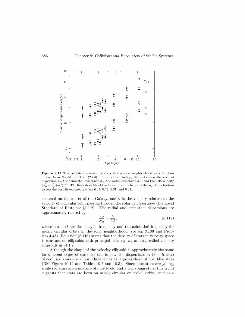
686 Chapter 8: Collisions and Encounters of Stellar Systems
Figure 8.11 The velocity dispersion of stars in the solar neighborhood as a functionof age, from Nordstrom et al. (2004). From bottom to top, the plots show the verticaldispersion !z , the azimuthal dispersion !!, the radial dispersion !R, and the rms velocity
(!2R +!2
! +!2z)1/2. The lines show fits of the form !i # t" where t is the age; from bottom
to top the best-fit exponents # are 0.47, 0.34, 0.31, and 0.34.
centered on the center of the Galaxy, and v is the velocity relative to thevelocity of a circular orbit passing through the solar neighborhood (the LocalStandard of Rest; see §1.1.2). The radial and azimuthal dispersions areapproximately related by
#%
#R=
)
2', (8.117)
where ) and ' are the epicycle frequency and the azimuthal frequency fornearly circular orbits in the solar neighborhood (see eq. 3.100 and Prob-lem 4.43). Equation (8.116) states that the density of stars in velocity spaceis constant on ellipsoids with principal axes #R, #% and #z, called velocityellipsoids in §4.1.2.
Although the shape of the velocity ellipsoid is approximately the samefor di!erent types of stars, its size is not: the dispersions #i (i = R,", z)of cool, red stars are almost three times as large as those of hot, blue stars(BM Figure 10.12 and Tables 10.2 and 10.3). Since blue stars are young,while red stars are a mixture of mostly old and a few young stars, this trendsuggests that stars are born on nearly circular or “cold” orbits, and as a

8.4 Encounters in stellar disks 687
stellar population ages it “heats up” in the sense that the dispersions #i
increase. This hypothesis can be confirmed by measuring the age-velocitydispersion relation for nearby stars (Figure 8.11). These observations showthat #i $ t", where & ! 0.5 for #z and & ! 0.3 for both #R and #%—theexponent is necessarily the same for these two dispersions, because they arerelated by equation (8.117).
We refer to the steady increase of these dispersions with time as diskheating, and in this section we investigate the dynamics of this process.A natural first step in this investigation is to wonder whether disk heatingcan be due to the accumulation of small velocity kicks from passing stars.This process was described briefly in §1.2.1 and more thoroughly in §7.4. Inparticular, in the discussion following equation (7.106) we saw that encoun-ters between stars in the solar neighborhood have a negligible e!ect on theirvelocities over the age of the Galaxy. Thus we must seek other explanations.
The simplest mechanism for disk heating is encounters with hypotheticalmassive objects in the dark halo, or machos. This process was investigatedin §7.4.4, where we found that the predicted time dependence of the velocitydispersion #R is incorrect. Moreover, the required macho mass appears tobe incompatible with observations of wide binary stars in the halo (§8.2.2e).We therefore examine other possibilities.
8.4.1 Scattering of disk stars by molecular clouds
Long before molecular clouds were detected, Spitzer & Schwarzschild (1951,1953) suggested that encounters between disk stars and massive gas cloudsmight be responsible for the random velocities of old disk stars. In Figure 8.12we illustrate how a molecular cloud or other mass m on a circular orbit in adisk a!ects the orbits of nearby stars. Since the cloud mass is &< 10"5 timesthe mass of the Galaxy, we may use Hill’s approximation (§8.3.2), in whichthe cloud is at rest at the origin of a rotating Cartesian coordinate system,with the x axis pointing radially outward and the y axis in the direction ofrotation. For simplicity we neglect motion perpendicular to the x–y plane.The stellar trajectories are given by the equations of motion (8.97), wherethe cloud potential &s = (Gm/(x2 + y2)1/2. In the figure, we write thedistances in terms of the Jacobi radius of the cloud (eq. 8.106),
rJ =
#Gm
4'0A0
$1/3
= 52 pc
#m
105 M!
'0
A0
$1/3 #220 km s"1
vc
R0
8 kpc
$2/3
.
(8.118)In these units, the equations of motion are independent of m, so Figure 8.12applies to clouds of any mass.
The figure shows only stars on initially circular orbits that are largerthan the cloud’s orbit. The behavior of orbits that are smaller than thecloud’s can be deduced by reflecting the orbits shown through the origin of

688 Chapter 8: Collisions and Encounters of Stellar Systems
Figure 8.12 The trajectories of stars near a mass point in a disk. The orbit of the masspoint is circular, as are the initial orbits of the stars. The coordinate frame co-rotates withthe mass point, which is therefore fixed at the origin; in this expanded view of the areanear the mass point, upwards is radially outward and the mass point is traveling to the leftin an inertial frame. All orbits are restricted to the z = 0 plane. Circular orbits appearas straight horizontal lines. A sequence of seven orbits is shown, all initially circular withradius slightly larger than that of the point mass, so it overtakes them. The behavior oforbits inside the point mass is given by reflecting these orbits through the origin. Thetrajectories of the stars are described by equations (8.97). The disk is assumed to havea flat circular-speed curve, so Oort’s constant A0 = $0/2 and the epicycle frequency$0 =
$2$0. Distances are measured in units of the Jacobi radius rJ of the mass point
(eq. 8.106), which is also the radius of the circle representing its location.
the figure. The initial orbits shown have angular speeds that are smaller thanthe cloud’s, so the cloud overtakes them (i.e., they move to the right in thecloud frame of reference that is used in the figure). If the initial di!erence inorbital radii "r &< rJ, the encounter simply reverses the direction of the orbitrelative to the cloud, without imparting any significant epicycle motion.11 If"r & rJ, the encounter imparts significant epicycle motion—the epicycleamplitude is comparable to "r and the encounter may or may not reversethe overall direction of motion of the orbit relative to the cloud. For "r &> rJ,the star passes the cloud and acquires a small epicyclic motion. It is thisexcitation of epicycle motion by encounters with clouds that warms the disk.
We may estimate the e#ciency of this process by using the impulseapproximation to find the radial velocity acquired by a star that is initiallyon a circular orbit of radius R. If Rc is the radius of the cloud orbit, thenin the sheared sheet the star’s initial orbit is x = R ( Rc * b = constant ,
11 This is an example of the donkey e"ect, described in Box 3.3. No epicycle motionis excited because the star approaches the cloud slowly, so its eccentricity is an adiabaticinvariant. For a comprehensive discussion of the trajectories in this problem, see Petit &Henon (1986).

8.4 Encounters in stellar disks 689
y(t) = constant ( 2A0bt (eq. 8.99). Integrating the gravitational attractionof the potential &s(x) along this trajectory yields
x = (" #
"#dt
Gmb
[b2 + y2(t)]3/2= (
Gm
A0b2. (8.119)
In the impulse approximation, immediately after the encounter we have
x = b ; x = (Gm
A0b2; y = (2A0b, (8.120)
and the corresponding epicycle energy and amplitude are given by equations(8.103),
"Ex = 12 x2 =
f2
2
#Gm
A0b2
$2
; X = fGm
A0)0b2, (8.121a)
where f = 1. We have introduced the correction factor f because the impulseapproximation is not accurate: since the radial velocity oscillates with theepicycle frequency )0, the impulse approximation requires that the durationof the encounter is much less than the epicycle period. In fact, the durationis " b/y = (2A)"1, which is comparable to the epicycle period 2!/)0. Hencethe impulse approximation makes an error of order unity in the epicycleenergy. The correct derivation (Julian & Toomre 1966 and Problem 8.20)yields
f ='0
A0K0
( )0
2A0
)+
)0
2A0K1
( )0
2A0
), (8.121b)
where K& is a modified Bessel function (Appendix C.7). For a flat circular-speed curve, A = 1
2', ) =)
2', and f = 0.923; for a Keplerian curvef = 1.680.
This result is based on linear perturbation theory, and hence is valid onlywhen the epicycle amplitude X induced by the encounter is much smallerthan the impact parameter b. Requiring that X &< b implies that
b
rJ&>
#4f'0
)0
$1/3
" 1, (8.122)
where we have used equation (8.118) for the Jacobi radius. Thus, equa-tions (8.121) are valid for encounters with impact parameters that are largecompared to the Jacobi radius, and they show that the epicycle energy ex-cited in an encounter falls o! as b"4. On the other hand, Figure 8.12 showsthat encounters at small impact parameters, b &< rJ, simply switch the starfrom one circular orbit to another, with no sensible increase in the star’srandom velocity. These considerations imply that the strongest encounters

690 Chapter 8: Collisions and Encounters of Stellar Systems
have b & rJ, and hence justify our treatment of the molecular cloud as apoint mass: since the typical cloud radius R & 10 pc is much smaller thanits Jacobi radius (8.118), the non-zero cloud size has little influence on therate of disk heating.
The speeds with which the stars in Figure 8.12 approach the scatter-ing cloud are due entirely to the di!erential rotation of the galactic disk,y = (2A0b. Once the stars have acquired non-zero epicycle energy, we haveto consider two types of encounter. For large impact parameters b or smallepicycle amplitudes X , the approach speed is still dominated by the con-tribution from di!erential rotation (shear-dominated encounters), but atimpact parameters b &< )0X/A0, the encounter geometry will be determinedmainly by the star’s epicyclic motion (dispersion-dominated encounters).
In contrast to shear-dominated encounters, dispersion-dominated en-counters usually can be treated using the impulse approximation. In thisapproximation, the magnitude of the velocity change "v in a single en-counter is proportional to v"1 where v is the encounter velocity. Thus theaverage change in epicycle energy Ex is proportional to v"2, and since thenumber of encounters per unit time is proportional to v and v2 & Ex weexpect (cf. Problem 8.21)
dEx
dt$ v"1 $
1)Ex
. (8.123)
Integrating this result we find that Ex $ t2/3 so the velocity dispersionv $ t" with & = 1
3 . This simple calculation somewhat overestimates therate of growth of the dispersion, since the thickness of the stellar disk islarger than the thickness of the cloud layer, so stars spend a smaller andsmaller fraction of their time in the cloud layer as the vertical dispersion, andthe resulting thickness of the stellar disk, continue to grow. The numericalcalculations described below are consistent with this argument, suggestingthat & ! 0.2–0.25 for heating by molecular clouds. This value is too lowto match the observations shown in Figure 8.11—just the opposite problemfrom macho-dominated heating, which gives an exponent that is too large(eq. 7.102).
We have shown that encounters with clouds “heat” the disk, in the sensethat the mean epicycle energy increases with time. It is instructive to askwhere this energy comes from, since the total energy or Jacobi integral ofthe star (eq. 8.104) is conserved during each encounter. The first of equa-tions (8.103) shows that in a razor-thin disk the di!erence in epicycle energyEx before and after the encounter is equal and opposite to the di!erence in12A0L2/B0; in most galactic potentials A0/B0 < 0 so we conclude that anincrease in Ex is accompanied by an increase in |L| or in |xg| (eq. 8.102),where xg is the di!erence in radius between the guiding center of the stellarorbit and the orbital radius of the molecular cloud. In words, the gravita-tional interaction with the cloud repels the stars, in the sense that their mean

8.4 Encounters in stellar disks 691
orbital radius is shifted away from the cloud. Thus the energy to heat thedisk comes from a redistribution of the surface mass density of the stars inthe disk; the cloud acts as a catalyst to expedite this redistribution of energybut does not contribute any of its own energy to the disk heating.
Numerous authors have estimated the rate at which star-cloud encoun-ters heat disks (Spitzer & Schwarzschild 1951, 1953; Jenkins 1992; Hanninen& Flynn 2002). The best estimate of the number density and masses ofmolecular clouds in the solar neighborhood leads to a rate of velocity-dispersion growth that is too small by a factor of two or more; but theheating rate is likely to be enhanced by the swing-amplified response orspiral wake induced in the stellar disk by the gravitational field from themolecular cloud, which can be several times more massive than the clouditself (Julian & Toomre 1966; Julian 1967).
These studies also show that the predicted ratio #z/#R of the verticaland radial dispersions is ! 0.6 (Ida, Kokubo, & Makino 1993), not far fromthe observed ratio of 0.5. However, the predicted age-velocity dispersionrelation is approximately a power law, #i $ t", with exponent & ! 0.2–0.25. This is significantly lower than the observed exponent, which is 0.3 for#R and #% and even larger for #z (Figure 8.11). This result suggests thatmolecular clouds are unlikely to be the primary cause of disk heating.
8.4.2 Scattering of disk stars by spiral arms
The disks of spiral galaxies are far from smooth. Gas, dust, and young starsare always concentrated into spiral arms. Spiral features are also found inthe old stars that make up most of the mass of galactic disks (§6.1.2), soit is natural to ask whether the gravitational fields of spiral features, likethe fields from molecular clouds, are able to heat galactic disks (Barbanis &Woltjer 1967).
Consider a weak spiral potential with pattern speed 'p,
&s(R,", t) = ,F (R) cos[f(R) + m"( 'pt], (8.124)
where , ' 1. To illustrate the e!ect of this potential on a stellar orbit, weshall make two assumptions that simplify the algebra but still retain mostof the important dynamics: (i) we work in the sheared-sheet approximation(§8.3.2); (ii) we consider only tightly wound spirals, for which the wavenum-ber k * df/dR is large compared to 1/R (eq. 6.4).
The sheared-sheet approximation is valid in a neighborhood of the diskcentered at a point [R0,"0(t)] that rotates at the circular angular speed"0 = '0 = '(R0). We expand the spiral potential in a Taylor series aroundthis point, using the coordinates x = R cos(" ( "0) ( R0 ! R ( R0 andy = R sin("( "0) ! R0("( "0). In this neighborhood, we can approximate

692 Chapter 8: Collisions and Encounters of Stellar Systems
the shape function as f(R) ! f(R0) + kx. Since the amplitude F (R) variesslowly, it can be replaced by a constant, F0 * F (R0). Thus we have
&s(x, y, t) = ,F0 cos[f(R0) + kx + my/R0 + m"0 ( 'pt]
= ,F0 cos[kx + my/R0 + m('0 ( 'p)t + constant].(8.125)
We now substitute this potential into the equations of motion (8.97) ofthe sheared sheet, neglecting motion in the z-direction perpendicular to thedisk plane:
x ( 2'0y ( 4'0A0x = ,kF0 sin[kx + my/R0 + m('0 ( 'p)t + constant];
y + 2'0x =,m
R0F0 sin[kx + my/R0 + m('0 ( 'p)t + constant].
Since the wave is assumed to be tightly wound, its pitch angle is small so|k| % m/R0 (eq. 6.7). Thus the right side of the second equation is muchsmaller than the corresponding term in the first, and can be neglected. Thesecond equation can then be integrated to yield y + 2'0x = constant , andthis can be substituted into the first equation to give
x+)20x+constant = ,kF0 sin[kx+my/R0+m('0('p)t+constant]; (8.126)
here )0 is the epicycle frequency (8.100). The constant on the left side can bedropped, since it can be absorbed by a shift in the origin of the x-coordinate.
In the absence of a spiral (F0 = 0) the solution to this equation isgiven by equations (8.99); we shall assume that the unperturbed motion iscircular, so the trajectory is x0(t) = (xg, yg0 ( 2A0xgt). Now consider howthis motion is modified by the weak spiral potential on the right side ofequation (8.126). We write the trajectory as x(t) = x0(t) + ,x1(t), where,x1(t) is the perturbation induced by the spiral. Then the terms of order ,in equation (8.126) yield
x1 + )20x1 = kF0 sin[kxg + m(yg0 ( 2A0xgt)/R0 + m('0 ( 'p)t + constant]
= kF0 sin(kxg + -t + c).(8.127)
In the last expression we have absorbed yg0 in the constant c, and set - =m('0 ( 2A0xg/R0 ( 'p); this is the frequency at which the unperturbedorbit encounters successive crests of the spiral potential.
This equation can be solved to yield
x1(t) =kF0
)20 ( -2
sin(kxg + -t + c). (8.128)
The solution diverges when - = ±)0. These points can be thought of as theLindblad resonances of the sheared sheet: at these locations, like the Lind-blad resonances in a disk, the frequency of excitation by the spiral potential

8.4 Encounters in stellar disks 693
coincides with the frequency )0 of the particle’s natural radial oscillation.This result is a close analog of equation (3.148), which was derived in thecontext of weak bars.
Equation (8.128) shows that the spiral potential imposes a forced radialoscillation on the star but does not lead to any steady growth in the radialoscillation x1(t). In other words, a spiral potential with a fixed pattern speedcannot heat the disk, except perhaps at the Lindblad resonances where oursimple derivation fails.
This result implies that disk heating requires transitory rather thansteady spiral patterns. To illustrate this, let us multiply the potential (8.124)or (8.125) by a Gaussian function of time, p(t) = (2!s2)"1/2 exp(( 1
2 t2/s2).Equation (8.127) is thereby modified to read
x1 + )20x1 = kF0p(t) sin(kxg + -t + c), (8.129)
which has the solution
x1(t) = X1 cos()0t +&1)+kF0
)0
" t
"#dt% p(t%) sin(kxg +-t% + c) sin[)0(t( t%)],
(8.130)where X1 and &1 are arbitrary constants. Inserting the chosen form for p(t)and setting the amplitude X1 of the free oscillation to zero, we obtain
x1(t . /) =kF0
2)0
5cos()0t ( kxg ( c)e"s2('+(0)
2/2
( cos()0t + kxg + c)e"s2('"(0)2/2
6.
(8.131)
Thus the transitory spiral pattern has induced a permanent epicyclic oscil-lation. When the characteristic duration of the transient, s, is much greaterthan the orbital period, the induced epicycle amplitude is strongly peakednear the Lindblad resonances - = ±)0. On the other hand, when the du-ration of the transient is short, the arguments of the exponential are smalland epicycle motion is induced over a wide range of radii in the disk.
This example shows that the ability of spiral structure to heat the diskis strongly dependent on its temporal structure. According to the Lin–Shuhypothesis (§6.1), in which spiral structure is a stationary wave with a single,well-defined pattern speed, disk heating is negligible except at the Lindbladresonances. In such models the disk can be heated over a wide range of radiionly if the pattern speed evolves with time, so the Lindblad resonances slowlysweep across most of the disk. On the other hand, if the spiral structure istransient, the whole disk can be heated—this situation is likely to occur inflocculent spirals, intermediate-scale spirals, or grand-design spirals excitedby recent encounters.
Let us suppose that a given star is subjected to N independent tran-sient perturbations. Each transient induces an epicyclic motion whose radial

694 Chapter 8: Collisions and Encounters of Stellar Systems
component can be written in the form x1(t) = ai cos()0t +&i), i = 1, . . . , N ,where ai and &i are given by equations similar to (8.131). After N transients,
x1(t) =N+
i=1
ai cos()0t + &i)
=(+
ai cos&i
)cos)0t (
(+ai sin&i
)sin)0t
* af cos()0t + &f)
(8.132)
where
a2f =
(+ai cos&i
)2+
(+ai sin&i
)2=
N+
i,j=1
aiaj cos(&i ( &j). (8.133)
Since the transients are uncorrelated, the phases of the epicyclic oscillationsthat they induce are also uncorrelated. Hence on average cos(&i ( &j) willbe zero when i 0= j, and the only terms in the sum that contribute to thefinal amplitude af will be those with i = j. Thus a2
f ! N+a2,, where +a2,is the mean-square amplitude induced by a single transient. If the rateof occurrence and the strength of new transients are independent of time,we conclude that a2
f , and hence the squared velocity dispersion v2, shouldgrow linearly with time. In other words, v $ t", where & = 0.5. Thisbehavior holds only so long as af is not too large: once the epicycle sizebecomes comparable to the radial wavelength of the spiral arms, the e!ectsof the spiral tend to average out over the epicycle period, so the heating isweaker—this is the same e!ect that leads to the reduction factor in the WKBdispersion relation for spiral waves, as described in §6.2.2d. Estimates of theheating rate at larger amplitudes can be obtained using the Fokker–Planckequation (Jenkins & Binney 1990; Jenkins 1992) or numerical simulations(De Simone, Wu, & Tremaine 2004); these calculations show that & can varybetween 0.25 and 0.5 depending on the properties of the spiral transients(duration, strength, pitch angle, etc.). This range of & is nicely consistentwith the observed exponent for the growth of the radial dispersion, & ! 0.3,and provides a substantially better fit than the values predicted for heatingby molecular clouds.
The radial and azimuthal velocity dispersions are related by equation(8.117), so the exponent in the age-velocity dispersion relation must be thesame for these two axes of the velocity ellipsoid. However, spiral structurecannot excite velocities in the z-direction e!ectively, since its spatial andtemporal scales are much larger than the amplitude or period of oscillationsperpendicular to the disk plane. Thus, scattering by spiral arms cannot ex-plain the relation between age and the z-velocity dispersion #z. Probablygravitational scattering by molecular clouds redistributes the radial and az-imuthal velocities into the direction perpendicular to the plane (Carlberg

8.5 Mergers 695
1987; Jenkins & Binney 1990). Thus molecular clouds are responsible forthe shape, but not the size, of the velocity ellipsoid.
Transient spiral arms have other interesting consequences for the dis-tribution of disk stars. Strong transients can produce long-lived clumps ofstars in velocity space, sometimes called star streams or moving groups (seepage 327 and De Simone, Wu, & Tremaine 2004). Spiral waves also re-distribute the angular momenta of disk stars, leading to substantial inwardand outward migration of individual stars over the lifetime of the Galaxy(Sellwood & Binney 2002).
8.4.3 Summary
There is little doubt that irregularities in the Galaxy’s gravitational field heatthe disk and thereby determine the velocity distribution of disk stars. It isless clear which irregularities dominate this process. We have discussed theinfluence of hypothetical massive objects in the dark halo (machos), molec-ular clouds, and transient spiral arms. Other possibilities include mergingsatellite galaxies (Walker, Mihos, & Hernquist 1996; Velazquez & White1999), substructure in the dark halo (Benson et al. 2004), or the Galacticbar (Kalnajs 1991; Dehnen 2000a). The simplest explanation that appears tobe consistent with most of the observations is the combined e!ects of spiraltransients and molecular clouds.
8.5 Mergers
So far we have investigated galaxy mergers and encounters through limitingcases that are analytically tractable. For example, minor mergers occurthrough dynamical friction (§8.1), which leads to gradual orbital decay, andas the orbit shrinks tidal forces and tidal shocks (§§8.2 and 8.3) becomestronger and stronger, until either the small galaxy is completely disruptedor its core comes to rest at the center of the larger galaxy.
In major mergers the physical processes are qualitatively similar, butharder to quantify. The relative velocity of the centers of mass of the twogalaxies is converted into randomly directed velocities of their individualstars—the same process as dynamical friction—but the conversion is so rapidthat the galaxies merge into a single steady-state system within a few crossingtimes. Thus, numerical simulations such as the one shown in Figure 8.1,rather than analytic arguments, are the primary tool for understanding majormergers.
In this section we shall focus on features of major mergers that havedirect observational consequences; these are important because they providethe “smoking gun” that enables us to identify galaxies that are participatingin ongoing mergers, and thus to explore the physics of mergers. Reviews

696 Chapter 8: Collisions and Encounters of Stellar Systems
of interacting and merging galaxies are given by Barnes & Hernquist (1992)and Kennicutt, Schweizer, & Barnes (1998).
8.5.1 Peculiar galaxies
A small fraction of galaxies are found in a highly disturbed state. Theimportance of these puzzling systems was emphasized by Arp (1966), whocompiled an Atlas of Peculiar Galaxies containing over 300 such objects (seealso Arp & Madore 1987). Arp argued that “if we could analyze a galaxyin a laboratory, we would deform it, shock it, probe it, in order to discoverits properties” and that the peculiarities of the galaxies in his atlas o!ered arange of experiments on galaxies furnished to us by nature, which we shouldlearn from. At one time it was widely believed that unusual systems of thiskind were exploding galaxies or galaxies with very strong magnetic fields, butby the early 1970s it became clear that most are actually colliding systems,and that many of these collisions will result in mergers.
Figure 8.13 shows the pair of galaxies NGC 4038/4039 from the Arp at-las. This system consists of overlapping blobs of light from which two curvedtails of much lower surface brightness emerge, giving rise to its commonname “the Antennae”. From end to end, the tails span over 100 kpc. Canthis striking morphology be the signature of a merger? In a classic paper,Toomre & Toomre (1972) showed that this is indeed the case. The Toomresstudied encounters between disks of massless particles orbiting around pointmasses: even with this grossly oversimplified model of a galaxy—the disk hasno self-gravity, there is no massive halo, and the disk circular-speed curveis Keplerian rather than flat—they were able to show that for a suitablechoice of initial conditions, it is possible to find a pair of colliding stellarsystems that is remarkably similar to Figure 8.13. We show their model inFigure 8.14. More accurate models that include the self-gravity of the diskand a massive halo largely confirm the Toomres’ conclusions (Barnes 1988;Dubinski, Mihos, & Hernquist 1999).
The Toomres’ model predicted the line-of-sight velocity at each point inthe system. The observed velocities were found to be in complete agreementwith the model, and show that the point of closest approach of the twogalaxies, when the tails were launched, occurred 0.5 Gyr ago (Hibbard et al.2001).
The tails seen in the Antennae di!er in one important respect from thetidal streamers discussed in §8.3.3. The streamers discussed in that sectionare composed of stars stripped from small satellites of much larger stellarsystems; the streamers are narrow because the satellite is small. In contrast,the two merging systems in the Antennae have comparable size; the tailsare narrow because the stars come from cold stellar systems—the disks ofthe two merging spiral galaxies—so all the stars near a given location havenearly the same initial velocity. Mergers of hot stellar systems of comparablesize do not generate narrow tidal tails.

8.5 Mergers 697
Figure 8.13 The interacting galaxies NGC 4038 and NGC 4039, the “Antennae”. Thisis an overexposed image to emphasize the low surface-brightness tidal tails. The distancefrom the overlapping blobs at the center to the bright star above and to the right of themis 40 kpc. Courtesy of D. F. Malin and the Anglo–Australian Telescope Board.
Another route to the same conclusion is through the collisionless Boltz-mann equation, which shows that the density of stars in phase space is con-served (eq. 4.10). A long-lived tidal tail or streamer must have high phase-space density, since the spatial density must be high if the tail is to be visibleagainst the background galaxy, and the velocity dispersion must be low if itis not to disperse quickly. Thus the progenitor of the tidal tail or streamermust have high phase-space density, a condition that is satisfied by bothsatellite stellar systems (because their spatial densities are high and theirvelocity dispersions are low compared to the larger host galaxy) and disks(because the velocity dispersion is low).
Another galaxy with prominent tidal tails that is almost certainly anongoing merger is NGC 4676 (“the Mice”), shown in Figure 8.15.

698 Chapter 8: Collisions and Encounters of Stellar Systems
Figure 8.14 A model of the NGC 4038/4039 pair by Toomre & Toomre (1972). Repro-duced by permission of The Astrophysical Journal.
8.5.2 Grand-design spirals
We have seen in Chapter 6 that grand-design spirals such as M51 (Plate 1)or M81 (Plate 8) often have companion galaxies nearby, and that the gravi-tational forces from an encounter with a companion can excite a strong buttransitory spiral pattern (Figure 6.26). In most cases the orbit of the com-panion galaxy that excited the spiral will decay by dynamical friction, sothe two galaxies are likely to merge in the future. Thus many of the mostbeautiful and striking spiral galaxies in the sky are likely to be the productof major mergers.

8.5 Mergers 699
Figure 8.15 The Mice, NGC 4676, a pair of interacting galaxies at a distance of 95Mpc.Top: optical image from the Hubble Space Telescope. Bottom: an N-body model. Creditfor HST image: NASA, H. Ford (JHU), G. Illingworth (UCSC/LO), M. Clampin (STScI),G. Hartig (STScI), the ACS Science Team, and ESA. Credit for N-body model: J. Dubinski(Dubinski & Farah 2006).
8.5.3 Ring galaxies
A handful of galaxies exhibit a distinctive morphology consisting of a lumi-nous ring of young stars that is both rotating and expanding, usually withone or more compact companion galaxies nearby. Figure 8.16 shows oneexample, the “Cartwheel Galaxy”. These remarkable systems are known asring galaxies or sometimes collisional ring galaxies (Appleton & Struck–Marcell 1996).12
Ring galaxies form when a disk galaxy collides head-on with anothersystem (Lynds & Toomre 1976). The collision excites a radially expanding
12 These are distinct from the prominent rings that are seen in some barred galaxies,which are thought to arise from rapid star formation in gas that is in resonance with thebar (see §6.5.2d and Buta 1995).

700 Chapter 8: Collisions and Encounters of Stellar Systems
Figure 8.16 The Cartwheel galaxy, the prototypical ring galaxy, at a distance of 125Mpc.The ring diameter is about 45 kpc. The lower of the two compact stellar systems to the leftof the ring—both members of the same group of galaxies as the Cartwheel—is probablyresponsible for the ring structure. Credit: K. Borne (George Mason University) andNASA.
density wave that triggers star formation in the disk as it passes. The com-pact systems are the surviving central cores of the colliding galaxies. Ringgalaxies are rare—about one in 104 galaxies—because they are short-lived,and because they are produced only in collisions with near-zero impact pa-rameter.
We can use the impulse approximation to develop an instructive modelof this process, even though this approximation may not hold for all ringgalaxies. Consider a singular isothermal sphere that contains a rotating,cold, disk of test particles in the plane z = 0, and suppose that it collideswith a second singular isothermal sphere having the same circular speed vc,traveling along the z axis with relative speed V % vc. The gravitationalpotential of each sphere is &(r) = v2
c ln r, and in Problem 8.7 it is shownthat the change "vR in the velocity of a disk star at initial radius R is then
"vR = (2Rv2c
V
" #
R
dr
r)
r2 ( R2= (
!v2c
V. (8.134)
If V/vc is su#ciently large, the velocity impulse "vR/vc will be small, so

8.5 Mergers 701
Figure 8.17 The evolution of theradii of particles in a disk after ahead-on encounter, as described byequation (8.135), following Toomre(1978). The ratio V/vc = 7.
(i) we may neglect the changes in the target’s potential that are generatedby the collision; (ii) we can describe the subsequent motion of the disk starsusing the epicycle approximation. If the collision is assumed to occur attime t = 0, the radius of a star that is initially at R0 is given by the solutionof equation (3.78a) that satisfies the initial conditions x(0) = R ( R0 = 0,x(0) = "vR:
R(R0, t) = R0 +"vR
)0sin()0t) (t > 0). (8.135)
Here )0 is the epicycle frequency at R0, which is given by )20 = 2v2
c/R20
(eq. 3.79a).The evolution of the radii of particles in the disk is shown in Figure 8.17.
The crowding of particle orbits gives rise to strong axisymmetric densitywaves that propagate out through the disk. The point of maximum compres-sion of the particle orbits is likely to be a region of enhanced star formation,which we identify with the ring of luminous young stars. The outward prop-agation of the density waves implies that the region inside the ring shouldcontain older, redder stars that were formed when the ring was smaller, andsuch radial color gradients are indeed observed in several ring galaxies.
In practice, the collision of two galaxies is never precisely along the z axisof the disk, as assumed in this simple model. However, numerical experimentssuch as those shown in Figure 8.18 show that whenever an intruder passesclose to the center of the target disk on a trajectory that is angled by less thanabout 30$ from the symmetry axis of the disk, a striking ring is generated.If the intruder misses the center of the target just slightly, the dense centerof the target galaxy is displaced from the center of the ring, as is observedin the Cartwheel Galaxy.
8.5.4 Shells and other fine structure
Figure 8.19 shows images of NGC 3923 and NGC 1344, which exhibit arclike

702 Chapter 8: Collisions and Encounters of Stellar Systems
Figure 8.18 Six encounters between a disk of test particles orbiting a point mass andan intruder of half the mass, marked by an open circle. The relative orbit is parabolic,and the system is viewed from 45" above the disk. A ring is generated when the impactparameter is small compared to the size of the disk (bottom three rows). From Toomre(1978), with permission of Springer Science and Business Media.

8.5 Mergers 703
Figure 8.19 The giant elliptical galaxies NGC 3923 (top) and NGC 1344 (bottom) aresurrounded by faint shells. The images have been processed to accentuate the shells usinga high-pass spatial filter. Courtesy of David Malin, c% Anglo–Australian Observatory.
shells in the surface brightness on both sides of the galaxy; careful analysisreveals over 20 such shells in this galaxy. The fraction of otherwise smooth

704 Chapter 8: Collisions and Encounters of Stellar Systems
Figure 8.20 The box and loop orbits shown in Figure 3.8. The upper figures show stars atrandomly chosen phases on the orbits to give a visual impression of the density distributionin the orbit, and the lower figures show the number of stars as a function of horizontalposition within the boxes marked by dashed lines. Note the sharp cusps at the turningpoints of the orbits.
galaxies (ellipticals and lenticulars) that exhibit shells can be as large as30–50%, depending on how closely one looks. Shells may also be present inspiral galaxies, but are camouflaged by spiral structure, dust, and irregularstar formation in the disk. Spectra show that the shells are composed of stars,not gas. As is often the case in astronomy, the most famous examples of thisphenomenon are atypical. The shells in NGC 3923 are exceptionally sharpand numerous, aligned with the major axis of the galaxy, and interleaved inradius (the shells from one side alternate in radius with those from the otherside). In contrast, most shell galaxies contain &< 3 detectable shells, andthese are fainter, more di!use, and have a less regular geometrical structure.
Other types of fine structure are also seen in elliptical galaxies (Kenni-cutt, Schweizer, & Barnes 1998), and are given names such as “loops”, “rip-ples”, “plumes”, “jets”, “X-structures”, etc. The tidal streamers describedin §8.3.3 are also a kind of fine structure.
Most fine structure in galaxies is formed by the same process that formstidal streamers, namely the disruption of a stellar system that has high phase-space density—either a small, hot galaxy or a large, cold one.
For example, consider the fate of the stars in a small satellite that isdisrupted by a host galaxy. Initially the disrupted stars will form a tidalstreamer, but eventually the streamer will disperse. If the host potentialis regular, the stars will finally spread into a cloud of particles that havesimilar actions but uniformly distributed angles. Such a cloud gives rise tosurface-density distributions such as those shown in Figure 8.20 for box andloop orbits. A box orbit produces an X-shaped structure, while a loop orbitproduces an annulus with sharp edges at its inner and outer turning points.

8.5 Mergers 705
In projection, the edges of these particle distributions can appear as shells,as indicated in the figure.
Another simple example is the disruption of a disk galaxy that is on aradial orbit in a spherical potential (Quinn 1984). This process can be ex-plored by releasing a cloud of test particles in a fixed potential (Figure 8.21).Since the angular momentum of the test particles is nearly zero, the motioncan be followed in the two-dimensional (r, vr) plane. Shells are formed at theturning points of the orbits, and they are interleaved in radius like the shellsobserved in NGC 3923. The rather special circumstances of the encounter(radial orbit, spherical host potential) are consistent with the observationthat most shell galaxies do not exhibit the regular geometrical structureseen in this example.
The much more common case of the disruption of a galaxy on a non-radial orbit can also produce shells, such as those shown in Figure 8.22, butnow the shells display the more complex geometry that is encountered inmost shell galaxies (Hernquist & Quinn 1988, 1989).
More generally, shells arise when stars are confined to a subspace of lowerdimensionality than the full six-dimensional phase space. The projection ofthis smooth manifold onto the two-dimensional plane of the sky gives rise tocaustics, which can be classified using catastrophe theory (Tremaine 1999).
8.5.5 Starbursts
So far we have focused on the e!ects of mergers on a galaxy’s stars, butthe e!ects on its gas—if the galaxy has a gas disk—are even more dramatic.As Toomre & Toomre (1972) wrote, “Would not the violent mechanical ag-itation of a close tidal encounter—let alone an actual merger—already tendto bring deep into a galaxy a fairly sudden supply of fresh fuel in the formof interstellar material?” The Toomres’ prescient question was answeredby Larson & Tinsley (1978), who showed that many merger remnants hadanomalous blue colors consistent with young, massive stars formed in a re-cent starburst—a short, intense period of rapid star formation at a ratefar exceeding that of a normal galaxy. Since that time a wide variety ofobservations has confirmed that vigorous star formation occurs in merginggalaxies. Among the most striking of these observations is the discovery ofalmost 103 blue objects in the Antennae (Figure 8.13), which appear to beyoung globular clusters formed in the merger (Whitmore & Schweizer 1995).
The observational link between mergers and star formation was ce-mented by the discovery of starburst galaxies. These are among the mostluminous galaxies known, emitting up to 1012.5 L!, mostly at infrared wave-lengths. This intense emission comes from young stars shrouded in dustand concentrated near the center of the galaxy. The emission is powered byextremely high star-formation rates, as large as 103 M! yr"1, compared toa few M! yr"1 in galaxies like the Milky Way. Starburst galaxies usually

706 Chapter 8: Collisions and Encounters of Stellar Systems
Figure 8.21 The disruption of a disk galaxy on a radial orbit in a spherical potential. Thehost galaxy is represented by a rigid, fixed Plummer potential (2.44a) with mass M = 1and scale length b = 1, and the satellite has mass m = 0.1 and is modeled by a rigidKuzmin-disk potential (2.68a) with scale length a = 0.5b, containing 10 000 test particleson initially circular orbits. Top: The cross marks the center of the host galaxy and thelength of each arm of the cross is 5b. The evolution is viewed from a direction normalto the plane of the disk galaxy (the x-y plane). The distribution of test particles is firstshown just before the satellite reaches the center of the host, falling in from infinity alongthe positive x axis, and at intervals of 10 time units thereafter. Bottom: the projection ofthe test particles onto the radius-radial velocity plane at time t = 50 (Quinn 1984).

8.5 Mergers 707
Figure 8.22 The formation of shells in the disruption of a small spherical galaxy on anon-radial orbit. The small ellipse in the first frame represents the approximate locationand projected shape of the larger galaxy in the encounter. The simulation uses 20 000 testparticles. From Hernquist & Quinn (1989), reproduced by permission of the AAS.
exhibit tidal streamers or other optical features indicative of a recent col-lision or merger (Sanders & Mirabel 1996; Kennicutt, Schweizer, & Barnes1998; Kennicutt 1998). The presence of these short-lived features, and therapid consumption of gas required by the high star-formation rate, imply

708 Chapter 8: Collisions and Encounters of Stellar Systems
that starbursts last for only a few tens of Myr.The reason for these very high star-formation rates is suggested by nu-
merical simulations of mergers of disk galaxies that contain both gas andstars (Noguchi 1988; Mihos & Hernquist 1996). During the merger, boththe gas and stars form strong bars. The gas bar leads the stellar bar, so thegravitational torque from the stars rapidly drains angular momentum fromthe gas. Remarkably, in a typical major merger the gas can lose up to 90%of its angular momentum in a fraction of an orbital period, thus settling intoa dense rotating disk &< 0.5 kpc across, in which star formation is likely to beextremely rapid.
8.5.6 The merger rate
The rate at which galaxies merge is a fundamental point of comparison be-tween observations and models of structure formation. The merger rate canbe determined from observations using two quite di!erent methods.
The first method is to count the fraction of galaxies showing obviousfeatures of an ongoing or recent major merger, such as tidal tails or star-bursts, and combine this fraction with an estimate of how long such featureslast to determine the merger rate per galaxy. The first attempt of this kindwas made by Toomre (1977b), who pointed out that about 10 of the & 4000NGC galaxies13 show prominent tidal tails, and that these tails probablylast no more than & 0.5 Gyr. Thus the rate of major mergers is probablyabout 10/4000/0.5 Gyr ! 0.005 Gyr"1 for a luminous galaxy. This estimateneglects two important biases, of opposite sign: first, not all major mergersyield visible tidal tails; second, mergers enhance the star-formation rate, sogalaxies experiencing mergers are more luminous than quiescent galaxies,and hence will be over-represented in a flux-limited catalog like the NGC. Acrude assumption is that these two biases cancel, leaving the original estimateof 0.005 major mergers per Gyr approximately correct.
A second approach is to count the fraction of galaxies with companionswithin a given radius, and combine this fraction with estimates of the rateof decay of the companion orbit by dynamical friction to obtain the mergerrate (Tremaine 1981). The distribution of companions is described by thegalaxy-galaxy correlation function .(r), defined so that the probabilityof finding two galaxies in the volumes d3r1 and d3r2 separated by r * |r1(r2|is
d2p = n20[1 + .(r)] d3r1d
3r2, (8.136)
where n0 d3r is the probability of finding one galaxy in the volume d3r. Overa wide range of separations and luminosities, the galaxy-galaxy correlation
13 NGC stands for “New General Catalog”, a catalog of galaxies, nebulae, and clusterscompiled by Dreyer in 1888, which was a revision and expansion of Herschel’s “GeneralCatalog” of 1864. See BM Appendix B.

8.5 Mergers 709
function can be described by a power law,
.(r) !(r0
r
)), (8.137)
where (Hawkins et al. 2003)
r0 = (7.2 ± 0.4)h"17 Mpc ; / = 1.67 ± 0.03, (8.138)
over the range 1 &< . &< 103. Thus the number density of companions atdistance r ' r0 from a primary galaxy is
n(r) = n0
(r0
r
)). (8.139)
The rate of decay of the orbital radius of a companion due to dynam-ical friction is given approximately by equation (8.16). Assuming that theprimary galaxy and the companion have similar luminosity and velocity dis-persion, #, we have
dr
dt! (0.4f#, (8.140)
where we have set the Coulomb logarithm ln % ! 1 according to the ar-guments that follow equation (8.17), and f &> 1 is a correction factor thatarises because the relative orbit is likely to be elongated rather than circular,which accelerates the decay. For each primary galaxy, the current of mergingcompanions through radius r is then
N(r) ! 12 # 4!r2n(r)
////dr
dt
//// ! 0.8!fn0#r)0 r2") ; (8.141)
the factor 12 is needed to avoid counting each galaxy twice, once as a primary
galaxy and once as a companion. In a steady state, the current should beindependent of r, and this constant number would represent the merger rate;the actual weak dependence on r seen in equation (8.141), N $ r2") $ r0.3,probably arises because our approximation that both galaxies are isothermalspheres is not very accurate. We shall equate the merger rate Nmerge toN(rmin), where rmin = 20h"1
7 kpc is roughly the radius at which the stellardistributions of two luminous galaxies begin to merge.
The derived merger rate depends on the minimum luminosity of thecompanion galaxies that we consider—clearly, if we count minor mergers,the merger rate will be higher than if we count only major mergers. For thepresent estimate we shall consider only mergers of companions with luminos-ity L > L!, where L! is the characteristic Schechter luminosity defined byequation (1.18). Using that equation, the average number density of galaxiesmore luminous than L! is
n0(L > L!) =
" #
L!
dL"(L) = "!
" #
1dxx"e"x. (8.142)

710 Problems
For the parameters given after equation (1.18), we find n0(L > L!) =0.21"! ! 1.0 # 10"3h3
7 Mpc"3. According to the Faber–Jackson law (1.21),the dispersion of an L! galaxy is #! ! 200 km s"1. Thus
Nmerge(L > L!) ! 0.8!fn0(L > L!)#!r)0 r2")
min
" 0.008h7f
2Gyr"1.
(8.143)
The approximate agreement of this estimate with the rate 0.005 Gyr"1 ob-tained by Toomre (1977b) provides encouraging evidence that our under-standing of the merging process is sound. More recent determinations of themerger rate (Conselice 2006) are also roughly consistent with these crudeestimates.
Problems
8.1 [1] Two identical galaxies are initially at rest, at a large distance from one another.They are spherical, composed solely of identical stars, and their light distributions obeythe Sersic law (1.17) with Sersic index m and e"ective radius Re. The galaxies fall togetherand merge. If the merger product also satisfies the Sersic law with the same index, whatis its e"ective radius?
8.2 [1] The derivation of the dynamical friction formula (8.1) assumes that the subjectsystem is a point mass, but in many cases of interest the subject system is an extendedbody, such as a star cluster or satellite galaxy, characterized by a median radius rh. If thepoint of closest approach of the field star to the center of the subject body is &< rh thenthe deflection of the field-star orbit, and its contribution to the drag force, will be smallerthan if the subject body were a point of the same total mass.
(a) Argue that the total drag force is largely una"ected by the non-zero size of the subjectbody if rh &< b90, where b90 is given by equation (3.51).
(b) If rh &> b90, argue that encounters with impact parameter &< rh make a negligiblecontribution to the total drag force. Using the first of equations (L.11), argue that in thiscase the argument of the Coulomb logarithm is given by % ! bmax/rh.
(c) Combine these conclusions to argue that the correct value of the argument of theCoulomb logarithm for a subject body of median radius rh is approximately
% =bmax
max(rh, GM/v2typ)
, (8.144)
and that the fractional error in ln% that arises from using this expression is of order(ln%)!1.
8.3 [3] In the core of a certain flattened elliptical galaxy, the mean stellar velocity van-ishes and the velocity distribution is Gaussian, with dispersion !z parallel to the galaxy’ssymmetry axis ez , and dispersion !# = !z/
$1 " e2 > !z in directions orthogonal to ez .
A massive body moves through the core at velocity v = vz ez + v#e#, where e# · ez = 0.Show that the frictional drag on the body may be written F = "%zvz ez "%#v#e#, where
1 <%z
%#=
I(1, 32 )
I(2, 12 )
; I(µ, &) 'Z $
1
d'
'µ(' " e2)#exp
h" 1
2!!2#
“v2#'
+v2
z
'" e2
”i. (8.145)
Hint: use the analogy between the Rosenbluth potential h(v) and the gravitational po-tential (see discussion following eq. L.19) and equation (2.125).

Problems 711
8.4 [3] Chandrasekhar’s dynamical friction formula can be derived using the linear re-sponse theory developed in §5.2.4 (Marochnik 1967; Kalnajs 1972b).
(a) Consider a point mass M traveling on the straight-line trajectory xM (t) = vM tthrough a uniform stellar system. Show that the spatial Fourier transform (eq. 5.26)of the density response is given by
(s1(k, t) = M
Zdt% R(k, t " t%) e!ik·vM t! , (8.146)
where R(k, ") is the response function (eq. 5.27).
(b) As we showed in §5.2.4, an infinite homogeneous stellar system is unstable, so toavoid an infinite response we must suppress the self-gravity of the system when evaluatingequation (8.146). The justification for this neglect is that the instability arises on scalescomparable to the Jeans length, while the dominant contribution to dynamical frictioncomes from encounters at much smaller distances (page 576), for which the e"ects ofself-gravity are small. To remove self-gravity, we simply replace the response functionR in equation (8.146) by the polarization function P , which measures the response toa given total potential rather than a given external potential. With this substitution,use equation (5.55) to show that if the stellar system has a Maxwellian df, the Fouriertransform of the density response is
(s1(k, t) = 4)GM( e!ik·vM tZ $
0d" "eik·vM $!(k%$)2/2, (8.147)
where ( and ! are the density and velocity dispersion of the host system.
(c) Take the inverse Fourier transform of (s1, and evaluate the resulting integrals to showthat the density response is
(s1(x, t) =GM(
!2rexp
"v2
M sin2 *
2!2
!»1 " erf
„vM cos *$
2!
«–, (8.148)
where erf denotes the error function (Appendix C.3), r = x " xM , r = |r|, and * is theangle between vM and r. Hint: carry out the integral over k first, using polar coordinatesin k-space with the polar axis along the vector r + vM" ; then evaluate the integral over" after transforming to the variable u = 1/" .
(d) Show that the gravitational force exerted on M by this density distribution is
F = 2)G2M2(
!2
vM
vM
Zdr
r
Z 1
!1dµ µ exp
"
"v2
M (1 " µ2)
2!2
# »1 " erf
„vM µ$
2!
«–, (8.149)
where µ = cos *.
(e) The upper limit to the integral over radius should be of order the size R of the hostsystem, while the lower limit should be roughly the 90" deflection radius b90 ( GM/!2
(eq. 3.51), since interior to this radius the perturbations to the orbits of passing stars areso large that linear response theory is invalid. With these limits, show that evaluationof the integrals in equation (8.149) yields the standard dynamical friction formula (8.7),with % = R/b90.
8.5 [1] At some initial time the stellar streaming velocity v(x) within an axisymmetricgalaxy of density ((R, z) constitutes circular rotation at angular frequency +(R, z). Thegalaxy is then perturbed by the high-speed passage of a massive system. Show thatwithin the impulse approximation the instantaneous change &v in v that is produced bythe encounter satisfies Z
d3x ((v ·&v) = 0. (8.150)
Hint: write v = +R e! and exploit the fact that &v can be derived from a potential.
8.6 [2] Reproduce Figure 8.4.

712 Problems
8.7 [2] Consider a high-speed head-on encounter at relative velocity V . Assume that theperturber is spherical, with gravitational potential #(r), and let (R, z) be cylindrical coor-dinates such that the z axis coincides with the perturber’s trajectory (i.e., the trajectoryis R = 0, z = V t).
(a) Show that the only non-zero component of the impulse to a star at (R, z) is
&vR = "2R
V
Z $
R
dr$
r2 " R2
d#
dr. (8.151)
(b) If the perturber is a Plummer model, # = "GM/$
r2 + b2, of mass M and scalelength b (§2.2.2c), show that the impulse is
&vR = "2GMR
V (R2 + b2). (8.152)
(c) If the perturber and the perturbed system are identical Plummer models, show thatthe energy per unit mass gained by each system in the encounter is
&E =G2M2
3V 2b2. (8.153)
8.8 [1] Show that the probability P (V ) dV that two stars drawn from Maxwellian dis-tributions with one-dimensional dispersions !1 and !2 have relative speed in the interval(V, V + dV ) is
P (V ) dV = (2)!2)!3/2 exp“"
V 2
2!2
”V 2dV, !2 = !2
1 + !22 . (8.154)
In words, the relative speed distribution is Maxwellian, with squared dispersion equal tothe sum of the squared dispersions of the two populations.
8.9 [1] Is there more angular momentum in the orbit of the Magellanic Clouds aroundour Galaxy or in the spin of the disk of our Galaxy?
8.10 [3] Show that the Lagrange points L4 and L5 in the restricted three-body problem
(a) each form an equilateral triangle with the two masses M and m.
(b) are stable if and only if the mass ratio m/(M + m) < 12"
$ 23108
= 0.03852 (Szebehely1967). Hint: start with equation (3.116); do not use equations (3.127) since these assumethat #xy = 0, which is not true in this case.
(c) Are the Lagrange points L1, L2, L3 stable?
8.11 [3] A frictionless railroad crosses a valley that separates two flat plateaus of equalheight. At t = 0, two cars, each of mass m, are sent o" with the same speed v andseparation d from the horizontal stretch of track on one side of the valley. Show that whenthe cars emerge onto the horizontal stretch of track on the other side of the valley, theyhave zero relative velocity and their separation is unchanged.
Discuss the relation between this system and disk shocking of globular clusters; inparticular, why does passage through the disk heat the cluster but leave the relativevelocity of the cars unchanged? Hint: consider adding a spring of rest length d andsti"ness +2/m between the two cars.
8.12 [2] A satellite system of mass m is in a circular orbit around a point-mass hostM ) m. Let (x, y, z) be Cartesian coordinates with ex pointing along the line joiningthe two masses and ez normal to the orbital plane. The distance of the tidal surface fromm along the x axis is rJ (eq. 8.91). Show that the distance of this surface from m alongthe y- and z-axes is 2
3 rJ and (32/3 " 31/3)rJ, respectively. Thus, the tidal surface is notspherical.

Problems 713
8.13 [2] In the distant-tide approximation, the tidal field around a freely falling satelliteof a host galaxy can be written in the form "!#t = "
P3i,j=1 ei#ijxj , where {xj} are
non-rotating Cartesian coordinates centered on the body (see §8.2.1). The tidal field issaid to be compressive along axis i if ei · !#t > 0, that is, if the tidal force pointstowards the center of the satellite.
(a) If the host galaxy is spherical with density (h(R) at a distance R from its center, provethat the tidal force is compressive along all three axes if and only if (h > 2
3(h, where (his the mean density of the host interior to R (cf. eq. 8.92).
(b) If the density of the host is ((R) # R!& , prove that the tidal force is compressive inall directions if and only if % < 1. In a host with this property tidal disruption cannotoccur, no matter how small the mass of the satellite may be. How is this result consistentwith the discussion of tidal disruption in §8.3?
8.14 [3] This problem investigates how orbits that lie far beyond the Jacobi radius canremain bound to a satellite. We consider a satellite on a circular orbit, using Hill’s ap-proximation (§8.3.2) and restrict our attention to the orbital plane of the satellite, z = 0.Since the orbits in question are much larger than the Jacobi radius, the gravitational fieldof the satellite is weak. Thus we may assume that the orbit is described approximately bythe solution (8.99) over timescales of order the epicycle period Tr = 2)/$0, with constantsof motion xg, yg0, X, Y , and , that change slowly due to perturbations from the satellite.
(a) Show that the guiding-center radius xg changes at a rate
xg =1
2B0
-#s
-y, (8.155)
where #s(x) = "Gm/(x2 + y2)1/2 is the potential from the satellite. Hint: use equations(8.97), (8.101), and (8.102).
(b) If the perturbations from the satellite are weak, and |xg| * |yg| (assumptions we willjustify below) then the term -#s/-y in equation (8.155) can be replaced by its averageover an epicycle period at fixed values of the constants of motion; that is
-#s
-y+fi
-#s
-y
fl'
Gm
2)
Z 2'
0d"
yg " Y sin "
[(xg + X cos ")2 + (yg " Y sin ")2]3/2. (8.156)
In the limit where |xg| * |yg| * X, that is, where the distance of the guiding center fromthe satellite is much less than the epicycle size, show thatfi
-#s
-y
fl= "
Gmyg
X3W
„$0
$0
«, where W (u) '
2
)
Z '/2
0d"
8u2 sin2 " " cos2 "
[cos2 " + 4u2 sin2 " ]5/2.
(8.157)Hint: expand equation (8.156) in a Taylor series, and use equation (8.100). The functionW (u) varies from 0.10032 for u = 1 (Keplerian orbits) to 0.22662 for u = 2!1/2 (flatcircular-speed curve) to 0.5 for u = 1
2 (harmonic oscillator).
(c) Di"erentiating the equation for yg(t) in (8.99) and using the assumption that the timederivatives of the constants of motion are small yields yg = "2A0xg. Using this resultand equation (8.155) show that the equation of motion for the guiding center is
yg = "A0
B0
fi-#s
-y
fl. (8.158)
Interpret this result in terms of the “e"ective mass” introduced in Box 3.3.
(d) Show that the motion of the guiding center is given by
xg(t) = Xg cos(+t + #) ; yg(t) = Yg sin(+t + #), (8.159)
where Xg and # are arbitrary and
Xg
Yg= "
+
2A0; +2 =
GmA0
"B0X3W
„$0
$0
«=
4$0A20
"B0
“ rJ
X
”3W
„$0
$0
«; (8.160)

714 Problems
the final form has been derived with the use of equation (8.106). In most galactic potentialsA0 > 0 and B0 < 0, so +2 > 0 and + is real. Thus the guiding center oscillates aroundthe satellite; if the orbit lies far outside the tidal radius (X ) rJ) then (i) the oscillationis slow in the sense that + * $0, and (ii) the excursions in yg are much larger than theexcursions in xg, consistent with the assumptions we made in deriving this result. Theapproximations we have used also require that Yg * Y , that is, the amplitude of theguiding-center oscillations must be smaller than the epicycle amplitude.
(e) In Problem 5.1, we showed that a solid ring orbiting a planet is unstable. This calcula-tion neglected tidal forces. Would a solid ring that is much larger than the Jacobi radiusbe stable?
8.15 [1] (a) Derive the energy integral (8.104) for the sheared sheet in two ways, first bymultiplying the equations of motion (8.97) by x, y, z respectively, adding, and integrating;second by finding the Lagrangian and Hamiltonian that yield the equations of motion.
(b) Assume that we impose periodic boundary conditions on the sheared sheet, by iden-tifying y + 2)R with y. Find the angle-action variables for the case #s = 0, and relatethese to the angle-action variables in the epicycle approximation (§3.5.3b).
8.16 [1] A spherical host galaxy contains two small satellites having masses m1 and m2.The satellites travel on nearly circular orbits with nearly the same orbital radius and plane.
(a) Argue that their interactions can be described using Hill’s approximation (8.97) in theform
x1"2$0y1"4$0A0x1 = "-#12
-x1; y1 +2$0x1 = "
-#12
-y1; z1 +$2
0z1 = "-#12
-z1, (8.161)
where #12 = "Gm2/|x1 " x2|. Here xi ' (xi, yi, zi) is the position of satellite i, i = 1, 2.The equation of motion for satellite 2 is obtained by interchanging the indices 1 and 2.
(b) In this approximation, what is the trajectory of the center of mass of the two satellites,xcm ' (m1x1 + m2x2)/(m1 + m2)?
(c) Show that determining the motion of the two satellites can be reduced to solving theequation of motion for a single particle with position x ' x2 " x1.
8.17 [2] This problem analyzes the sheared sheet (§8.3.2) as a model for the kinematicsof the solar neighborhood or other stellar disks. For simplicity, we restrict ourselves to atwo-dimensional disk, ignoring motion in the z-coordinate, although the results are easilygeneralized to three-dimensional disks.
(a) Show that in the absence of local mass concentrations (that is, if the satellite potential#s = 0) the equations of motion (8.97) are invariant under the transformation
x , x +&x ; y , y " 2A0&xt. (8.162)
Describe the physical meaning of this symmetry.
(b) According to the Jeans theorem, the equilibrium df f(x, y, x, y) can depend only onthe integrals of motion E& and L (eq. 8.101). Show that the only combination of theseintegrals that is invariant under the transformation (8.162) is the epicycle energy definedin equation (8.103). Thus argue that if the disk is smooth on small scales, the df musthave the form f(Ex).
(c) For a df of this form, show that the surface density is independent of position, themean radial velocity vanishes, the mean azimuthal or y-velocity is "2A0x, and the ratioof the dispersions in the azimuthal and radial directions is
!2y
!2x
=
Rdxdy f(Ex)(y + 2A0x)2R
dxdy f(Ex)x2=
$20
4$20
, (8.163)
a result already derived by di"erent methods in equation (3.100).

Problems 715
(d) Show that if f(Ex) # exp("E2x/!2
0) then
f(x, y, x, y) ='
)!20
$0
$0exp
»"
x2
2!20
"2$2
0(y + 2A0x)2
$20!
20
–. (8.164)
Show that this is the analog of the Schwarzschild df introduced in §4.4.3.(e) Does this df exhibit asymmetric drift (§4.8.2a)?
8.18 [2] Assume that the Sun travels in a circular orbit in the Galactic plane. Let (x, y, z)be rotating Cartesian coordinates centered on the Sun, with ex pointing away from theGalactic center and ez pointing to the north Galactic pole.
(a) Show that the zero-velocity surfaces in the combined gravitational field of the Sun andthe Galaxy are given by
2A(B " A)x2 + (A2 " B2 + 2)G(0)z2 "GM'
r= constant, (8.165)
where (0 is the density in the solar neighborhood, A and B are Oort’s constants, andr2 = x2 + y2 + z2. Hint: see Problem 3.18.
(b) Let xJ, yJ, zJ be the intersections of the Sun’s tidal surface with the coordinate axes.Evaluate these quantities in parsecs, using the parameters in Tables 1.1 and 1.2.
8.19 [2] Reproduce Figure 8.8.
8.20 [3] The goal of this problem is to determine the epicycle amplitude induced in astar as it passes a molecular cloud, in the shear-dominated regime. We use the equationsof motion (8.97) and neglect motion perpendicular to the x–y plane. We assume thatthe cloud is at the origin and that the star is initially on a circular orbit with impactparameter b, so x(t) = (b,"2A0bt). If the cloud potential is .(x) = "Gm/(x2 + y2)1/2
and its mass is su!ciently small that the right sides of the equations of motion can beevaluated along the unperturbed stellar orbit, show that after the encounter the epicycleamplitude is (Julian & Toomre 1966)
X =Gm$0
$0A20b2
»K0
„$0
2A0
«+
$0
2$0K1
„$0
2A0
«–, (8.166)
where K# is a modified Bessel function (Appendix C.7). Thus, derive the correction factorf in equation (8.121b).
8.21 [2] In this problem we estimate the rate of growth of epicycle energy in the dispersion-dominated regime. Consider a star traveling on a nearly circular orbit in the equatorialplane of a razor-thin galaxy. At time zero, the star is instantaneously deflected by thegravitational field from a nearby molecular cloud that is itself on a perfectly circular orbit.The star is traveling at speed v with respect to the cloud, and the encounter deflects itthrough an angle / onto a new, nearly circular orbit within the galactic plane. Show thatthe deflection changes the star’s epicycle energy by an amount
&Ex = Ex(%2 " 1)ˆsin2 /(sin2 #" %!2 cos2 #) "
1
2%sin 2/ sin 2#
˜, (8.167)
where % = 2$/$ and # is the epicycle phase (see eqs. 3.91 and 3.93, or 8.99). At theradius of the star’s orbit, there are n clouds per unit area, each having mass m. The massdistribution in the clouds can be represented by a Plummer model with scale length b,which is much smaller than the star’s epicycle radius. Using the impulse approximation,assuming that the relative velocity is dominated by the velocity dispersion of the stars,and assuming that the deflection angle / is small, show that the expectation value of therate of change of epicycle energy is
Ex =
$2G2m2n
b$
Ex(%2 " 1)
Z '/2
0d#
sin2 #" %!2 cos2 #
(sin2 # + %!2 cos2 #)3/2. (8.168)
Verify that Ex > 0 for % > 1. What happens to stars in a galaxy with % < 1?