collecting and handling point pattern data ebook.spatstat.org/sample-chapters/chapter03.pdf · e...

SAMPLE

3

Collecting and Handling Point Pattern Data

This Chapter provides guidance on collecting spatial data in surveys and experiments (Section 3.1),wrangling the data into files and reading it into R (Sections 3.2 and 3.9–3.10), handling the datain spatstat as a point pattern (Section 3.3), checking for data errors (Section 3.4), and creating aspatial window (Section 3.5), a pixel image (Section 3.6), a line segment pattern (Section 3.7), or acollection of spatial objects (Section 3.8).

3.1 Surveys and experiments

Every field of research has its own specialised methods for collecting data in surveys, observationalstudies, and experiments. We do not presume to tell researchers how to run their own studies.1

However, statistical theory gives very useful guidance on how to avoid fundamental flaws in thestudy methodology, and how to get the maximum information from the resources available.2 In thissection we discuss some important aspects of data collection, draw attention to common errors, andsuggest ways of ensuring that the collected data can serve their intended purpose.

3.1.1 Designing an experiment or survey

The most important advice about designing an experiment is to plan the entire experiment, includingthe data analysis. One should think about the entire sampling process that leads from the real thingsof interest (e.g., trees in a forest with no observers) to the data points on the computer screen whichrepresent them. One should plan how the data are going to be analysed, and how this analysis willanswer the research question. This exercise helps to clarify what needs to be done and what needsto be recorded in order to reach the scientific goal.

A pilot experiment is useful. It provides an opportunity to check and refine the experimentaltechnique, to develop protocols for the experiment, and to detect unexpected problems. The datafor the pilot experiment should undergo a pilot data analysis which checks that the experiment iscapable of answering the research question, and provides estimates of variability, enabling optimalchoice of sample size. Experience from the pilot experiment is used to refine the experimental pro-tocol. For example, a pilot study of quadrat sampling of wildflowers might reveal that experimenterswere unsure whether to count wildflowers lying on the border of a quadrat. The experimental pro-tocol should clarify this.

Consideration of the entire sampling process, leading from the real world to a pattern of dotson a screen, also helps to identify sources of bias such as sampling bias and selection effects. Ina galaxy survey in radioastronomy, the probability of observing a galaxy depends on its apparentmagnitude at radio wavelengths, which in turn depends on its distance and absolute magnitude. Bias

1“Hiawatha, who at college/ Majored in applied statistics,/ Consequently felt entitled/ To instruct his fellow man/ In anysubject whatsoever” [374]

2“To consult the statistician after an experiment is finished is often merely to ask him to conduct a post mortem examina-tion. He can perhaps say what the experiment died of.” R.A. Fisher

49

SAMPLE

50 Spatial Point Patterns: Methodology and Applications with R

of this known type can be handled during the analysis. In geological exploration surveys, unevensurvey coverage or survey effort introduces a sampling bias which cannot easily be handled duringanalysis unless we have information about the survey effort.

Ideally, a survey should be designed so that the surveyed items can be revisited to cross-checkthe data or to collect additional data. For example, GPS locations or photographic evidence couldbe recorded.

3.1.2 What needs to be recorded

In addition to the coordinates of the points themselves, several other items of information need tobe recorded. Foremost among these is the observation window, that is, the region in which the pointpattern was mapped. Recording the boundaries of this window is important, since it is a crucial partof the experimental design: there is information in where the points were not observed, as well asthe locations where they were observed.

Even something as simple as estimating the intensity of the point pattern (average number ofpoints per unit area) depends on the window of observation. Attempting to infer the observationwindow from the data themselves (e.g., by computing the convex hull of the points) leads to ananalysis which has substantially different properties from one based on the true observation window.An analogy may be drawn with the difference between sequential experiments and experiments inwhich the sample size is fixed a priori. Analysis using an estimated window could be seriouslymisleading.

Another vital component of information to be recorded consists of spatial covariates. A ‘co-variate’ or explanatory variable is any quantity that may have an effect on the outcome of the exper-iment. A ‘spatial covariate function’ is a spatially varying quantity such as soil moisture content,soil acidity, terrain elevation, terrain gradient, distance to nearest road, ground cover type, regionclassification (urban, suburban, rural), or bedrock type. More generally, a ‘spatial covariate’ is anykind of spatial data, recruited as covariate information (Section 1.1.4). Examples include a spatialpattern of lines giving the locations of geological faults, or another spatial point pattern.

A covariate may be a quantity whose ‘effect’ or ‘influence’ is the primary focus of the study.For example in the Chorley-Ribble data (see Section 1.1.4, page 9) the key question is whether therisk of cancer of the larynx is affected by distance from the industrial incinerator. In order to detecta significant effect, we need a covariate that represents it.

A covariate may be a quantity that is not the primary focus of the study but which we need to‘adjust’ or ‘correct’ for. In epidemiological studies, measures of exposure to risk are particularly im-portant covariates. The density of the susceptible population is clearly important as the denominatorused in calculating risk. A measure of sampling or censoring probability can also be important.

Theoretically, the value of a covariate should be observable at any spatial location. In reality,however, the values may only be known at a limited number of locations. For example the valuesmay be supplied only on a coarse grid of locations, or measured only at irregularly scattered samplelocations. Some data analysis procedures can handle this situation well, while others will require usto interpolate the covariate values onto a finer grid of locations.

The minimal requirement for covariate data is that, in addition to the covariate values at all pointsof the point pattern, the covariate values must be available at some ‘non-data’ or ‘background’

locations. This is an important methodological issue. It is not sufficient to record the covariate

values at the data points alone.

For example, the finding that 95% of kookaburra nests are in eucalypt trees is useless untilwe know what proportion of trees in the forest are eucalypts. In a geological survey, suppose wewish to identify geochemical conditions that predict the occurrence of gold. It is not enough torecord the geochemistry of the rocks which host each of the gold deposits; this will only determinegeochemical conditions that are consistent with gold. To predict gold deposits, we need to findgeochemical conditions that are more consistent with the presence of gold than with the absence of

SAMPLE

Collecting and Handling Point Pattern Data 51

gold, and that requires information from places where gold is absent. (Bayesian methods make itpossible to substitute other information, but the basic principle stands.)

There are various ways in which a covariate might be stored or presented to a spatstat functionfor analysis. Probably the most useful and effective format is a pixel image (Section 3.6).

It is good practice to record the time at which each observation was made, and to look forany apparent trends over time. An unexpected trend suggests the presence of a lurking variable

— a quantity which was not measured but which affects the outcome. For instance, experimentalmeasurements may depend on the temperature of the apparatus. If the temperature is changingover time, then plotting the data against time would reveal an unexpected trend in the experimentalresults, which would help us to recognise that temperature is a lurking variable.

3.1.3 Risks and good practices

The greatest risk when recording observations is that important information will be omitted or lost.Charles Darwin collected birds from different islands in the Galapagos archipelago, but failed torecord which bird came from which island. The missing data subsequently became crucial for thetheory of evolution. Luckily Darwin was able to cross-check with the ship’s captain, who hadcollected his own specimens and had kept meticulous records.

What information will retrospectively turn out to be relevant to our analysis? This can be diffi-cult to foresee. The best insurance against omitting important information is to enable the obser-

vations to be revisited by recording the context. For example when recording wildflowers insidea randomly positioned wooden quadrat in a field, we could easily use a smartphone to photographthe quadrat and its immediate environment, and record the quadrat location in the field. This willat least enable us to revisit the location later. Scientific instincts should be trusted: if you feel thatsomething might be relevant, then it should be recorded.

In particular don’t discard recorded data or events. Instead annotate such data to say they‘should’ be discarded, and indicate why. The data analysis can easily cope with such annotations.This rule is important for the integrity of scientific research, as well as an important precaution foravoiding the loss of crucial information.

Astronomers sometimes delete observations randomly from a survey catalogue to compensatefor bias. For example, the probability of detecting a galaxy in a survey of the distant universedepends on its apparent brightness, which depends on its distance from Earth. Nearby galaxieswould be overrepresented in a catalogue of all galaxies detected in the survey. Common practice isto delete galaxies at random from the survey catalogue, in such a way that the probability of retaining(not deleting) a galaxy is inversely proportional to the sampling bias (the conjectured probabilityof observing the galaxy). In some studies the randomly thinned catalogue becomes ‘the’ standardcatalogue of galaxies from the survey. We believe this is unwise, because information has been lost,and because this procedure is unnecessary: the statistical analysis can cope with the presence ofsampling bias of a known type. In other studies, the random thinning is done repeatedly (startingeach time from the original observations); this is valid and is an application of bootstrap principles[316].

A particular danger is that events may be effectively deleted from the record when their spatiallocation ceases to exist. For example, in road traffic accident research, the road network changesfrom year to year. If a four-way road intersection has been changed into a roundabout, should trafficaccidents that occurred at the old intersection be deleted from the accident record? If we did (or ifthe database system effectively ignored such records), it would be impossible to assess whether thenew roundabout is safer than the old intersection.

Where data are missing, record the ‘missingness’. That is, if no value is available for a particularobservation, then the observation should be recorded as ‘NA’. Moreover when recording the ‘miss-ingness’ be sure to use proper missing value notation — do not record missing values as supposedlyimplausible numerical values such as ‘99’ or ‘−99’. Doing so can have disastrous results in the

SAMPLE


analysis. Likewise do record ‘zeroes’ — e.g., zero point counts for quadrats in which no pointsappear. Do not confuse these two ideas: ‘missing’ or ‘unobservable’ (NA) is a completely differentconcept from ‘absent’ (0).

Data should be recorded at the same time as the observation procedure; record as you go. Ifwriting observations down on paper or tablet is not feasible, use a recording device such as a mobilephone. A photograph of the immediate environment can also be taken with a mobile phone.

In accordance with Murphy’s Law, it is imperative to keep backups of the original data, prefer-ably in text files. Data that are stored in a compressed or binary format, or in a proprietary formatsuch as a word-processing document, may become unreadable if the format is changed or if theproprietary software is updated.

To ensure good practice and forestall dispute, conditions for accessing the data should be clari-fied. Who owns the data, who has permission to access the data, and under what conditions? Privacyand confidentiality restrictions should be clarified.

Data processing (including reorganising and cleaning data) should be documented as it happens.Record the sequence of operations applied to the data, explain the names of variables, state the unitsin which they are expressed, and so on. Data processing and cleaning can usually be automated,and is usually easy to implement by writing an R script. The script effectively documents what youdid, and can be augmented and clarified by means of comments.

Data analysis should also be documented as it happens. We strongly recommend writing R

scripts for all data analysis procedures: this is easier in an environment such as RStudio or ESS.The interactive features of R are very handy for exploring possibilities, and it does provide a basicmechanism for recording the history of actions taken. The disadvantage is that it can be difficultto ‘back out’ (to return to an earlier stage of analysis) and the analysis may depend on the state ofthe R workspace. Once you have figured out what to do, we strongly advise writing code (withcopious comments!) that performs the relevant steps from the beginning. This makes the analysisreproducible and verifiable.

3.2 Data handling

3.2.1 Data file formats

If you obtain data files from another source, such as a website, it is of course important to understandthe file format in which the data are stored and to have access to the software needed to extract thedata from the files in question. It is also important to obtain all of the available information aboutthe protocols under which the data were gathered, the range of possible values for each variable, theprecision to which the variables were recorded, whether measurements were rounded and if so how,the taxonomic system or nomenclature used, and the treatment of missing values. See Chapter 4 forsome advice on these matters.

If you have collected data yourself it is, as was mentioned above, good practice to save theoriginal data in a text file, so that it is not dependent on any particular software. The text file shouldhave a clearly defined format or structure. Data in a text file can easily be read into R.

For storing the point coordinates and associated mark values (see Section 3.3.2 for a discussionof marks) we recommend the following file formats.

table format: the data are arranged in rows and columns, with one row for each spatial point. Thereis a column for each of the x- and y-coordinates, and additional columns for mark variables. SeeFigure 3.1. The first line may be a header giving the names of the column variables.

Character strings must be enclosed in quotes unless they consist entirely of letters. Missing values

SAMPLE


should be entered as NA. The usual file name extension is .txt or .tab (the latter is understoodby R to indicate that the file is in table format).

comma-separated values (csv): Spreadsheet software typically allows data to be exported to orimported from a comma-separated values file (extension . sv). This format is slightly morecompressed than table format. Data values are separated by a comma (or other chosen character)rather than by white space. This format is convenient because it is widely accepted by othersoftware, and is more memory-efficient than table format. However, errors are more difficult todetect visually than they are in table format.

shapefiles: A shapefile is a popular file format for sharing vector data between geographic infor-mation system (GIS) software packages. It was developed and is maintained by the commercialsoftware provider ESRI™. Most of the specification is publicly accessible [254]. Storing data in ashapefile will result in a handful of files, with different extensions (at least .shp, .shx, and .dbf)which refer to different information types, e.g., the coordinates and the geographical projectionthat was used. Reading data from shapefiles is described in Section 3.10.

Easting Northing Diameter Spe ies

176.111 32.105 10.4 "E. regnans"

175.989 31.979 7.6 "E. amaldulensis"

.... .... ....

Figure 3.1. Example of text file in table format.

You will also need to store auxiliary data such as the coordinates of the (corners of the) windowboundary, covariate data such as a terrain elevation map, and metadata such as ownership, physicalscale, and technical references. The window boundary and covariate data should also be stored intext files with well-defined formats: we discuss this in Section 3.5. Metadata can usually be typedinto a plain text file with free format.

3.2.2 Reading data into R

Data in a text file in table format can be read into R using the command read.table. A comma-separated values file can be read into R using read. sv. Set the argument header=TRUE if the filehas a header line (i.e. if the first line of the file gives the names of the columns of data).

The original data files for the vesi les dataset are installed in spatstat as a practice example.To copy these files to the current folder, type

> opyExampleFiles("vesi les")

The coordinates of the vesicles can then be read by either of the commands

> ves <- read.table("vesi les.txt", header=TRUE)

> ves <- read. sv("vesi les. sv")

The resulting object ves is a ‘data frame’ in R. You may need to set various options to get thedesired result: type help(read. sv) or help(read.table) for information.

Use olnames(ves) to see the names of the columns in the data frame ves: these may havechanged if the original column names contained strange characters or were duplicated. Note that if

SAMPLE


the original data file had no header line, the columns of the data frame will have the default namesV1, V2, .... Use head(ves) to see the first few rows of data, and summary(ves) to see asummary of the values in each column of the data frame. See Section 2.1.6 for more on data frames.

It is important to check that each column of data belongs to the intended class. Note that a col-umn of character strings in the text file will be converted to a factor (categorical variable) by default.Conversion to a factor would probably be appropriate for the Spe ies column in Figure 3.1. How-ever, character strings could also represent date-and-time values, or text annotations. In this caseread.table or read. sv should be called with stringsAsFa tors=FALSE to prevent automaticconversion to factors (or options should be used to change the default behaviour); then each col-umn should be converted to the desired type. Factors are created using fa tor or as.fa tor. Formore details on factors see Section 2.1.9. Strings representing date-time values are converted usingas.Date or as.POSIX t. For more details on handling dates in R see the help entries for ISOdateand ISOdatetime, or the online resources [578], www.statmethods.net/input/dates.htmlor en.wikibooks.org/wiki/R_Programming/Times_and_Dates.

Note that if a column of numbers in the text file has been ‘corrupted’ with non-numeric charac-ters — possibly due to typing errors — then this column will be read in as character data (and thenby default converted to a factor). Checking on the class of each column serves to detect when sucherrors have occurred. A quick and easy way to find out the class of data in each column of your dataframe df is sapply(df, lass). If conversion errors are found, the text file should be corrected,and read in again. Alternatively the data frame can be viewed and edited in a spreadsheet-styleinterface using the R functions View and edit.

3.3 Entering point pattern data into spatstat

A spatial point pattern in two-dimensional space is stored in spatstat as an object of class "ppp"(for ‘planar point pattern’). In order to use the capabilities of spatstat, a spatial point patterndataset should be converted into an object of this class.

A point pattern object contains the spatial coordinates of the points, the marks attached to thepoints (if any), the window in which the points were observed, and the name of the unit of length forthe spatial coordinates. Thus, a single object of class "ppp" contains all the information required toperform standard calculations about a point pattern dataset.

This section describes some basic ways to create "ppp" objects from raw data, or from datastored in a text file. For data stored in a recognised GIS file format, alternative methods are describedin Section 3.10. Section 3.9 explains how to create a point pattern interactively using a point-and-click interface, which can be useful when the original dataset is a digital photograph or another formof spatial data.

3.3.1 Creating a "ppp" object

To create an object of class "ppp" from raw data, use the function ppp. Suppose that the x,ycoordinates of the points of the pattern are contained in vectors x and y (which must, of course, beof equal length). Then

X <- ppp(x, y, other.arguments)

will create the point pattern object X. The other.arguments must determine a window for thepattern. Table 3.1 shows the different options for specifying a window.

If the observation window is a rectangle, it is sufficient to specify the ranges of the x and y

coordinates:

SAMPLE


ppp(x, y, xrange, yrange) point pattern in rectangleppp(x, y, poly=p) point pattern in polygonal windowppp(x, y, mask=m) point pattern in binary mask windowppp(x, y, window=w) point pattern in specified window

Table 3.1. Basic options for creating a point pattern using the creator function ppp.

> df <- read.table("vesi les.txt", header=TRUE)

> x <- df$x

> y <- df$y

> X <- ppp(x, y, (22,587), (11,1031))

or more compactly

> X <- with(df, ppp(x, y, (22,587), (11,1031)))

If the argument window is given, then it must be a window object (of class "owin") specifying thewindow for the point pattern. Otherwise, the additional arguments are passed to the function owinto create a window object. Section 3.5 gives a detailed explanation of these arguments.

Often the window of observation is a rectangle, so this requirement just means that we have tospecify the x and y dimensions of the rectangle when we create the point pattern. Windows with amore complicated shape can easily be represented in spatstat, as described below.

The term ‘window of observation’ presumes that the points are scattered in two-dimensionalspace but that observations were confined to a known study region (‘Window Sampling’, page 143).This may not be appropriate in some applications. However, many statistical techniques still requiresome kind of bounding region for the point pattern. If the points are confined to a bounded region ofspace, like fish in a lake, the ‘Small World’ model (page 145) is more appropriate. If the boundingregion is really unknown, spatstat provides the function ripras to compute the Ripley-Rasson[580] estimator of the bounding region, given only the point locations.

After creating a point pattern object X, it is advisable to type X to print the object, is.ppp(X) tocheck that it is indeed a point pattern, summary(X) to summarise its contents, and plot(X) to plotthe pattern. More about these commands is explained in Chapter 4.

The generic functions View and edit also have methods for "ppp" objects, allowing the userto inspect and edit the spatial coordinates in a spreadsheet-like interface.

3.3.2 Marks

Chapter 1 introduced the idea of a ‘mark’, an additional attribute of each point in a point pattern.For example, in addition to recording the locations of trees in a forest, we could also record thespecies, diameter, and height of each tree, a chemical analysis of the leaves of each tree, and so on.

Suppose x and y are vectors containing the coordinates of the point locations, as before, andfor simplicity assume that the observation window is a rectangle with extent given by xrange andyrange. If there are marks attached to the points, store the corresponding marks in a vector m withone entry for each point or in data frame m with one row for each point and one column for eachmark variable. (It is also possible to use a matrix rather than a data frame to store multiple marks,but such a matrix is just converted to a data frame internally by ppp and in general a data frame ispreferred.) Then create the marked point pattern by

ppp(x, y, xrange, yrange, marks=m)

For example, the following code reads raw data from a text file in table format, and creates a pointpattern with a column of numeric marks containing the tree diameters:

SAMPLE


> opyExampleFiles('finpines')

> fp <- read.table('finpines.txt', header=TRUE)

> X <- with(fp, ppp(x, y, (-5,5), (-8,2), marks=diameter))

An even slicker way to do this is to convert the data frame directly into a point pattern using theconversion operator as.ppp:

> fp <- read.table("finpines.txt", header=TRUE)

> X <- as.ppp(fp, owin( (-5,5), (-8,2)))

Notice this requires that the first two columns of fp contain the x and y coordinates (which they doin this case). The two steps of reading in data and creating an object of class "ppp" can be reducedto one step by using s anpp:

> X <- s anpp("finpines.txt", owin( (-5,5), (-8,2)))

The handling of marks in spatstat depends on their type. Mark values may belong to any of theatomic data types: numeric, integer, character, logical, or complex. Marks may also be categoricalvalues (see below), calendar dates, or date/time values. Character-valued marks are rarely used;they should usually be converted to categorical or date/time values. To check that your data has theintended type, use lass(m) if m is a vector and sapply(m, lass) if m is a data frame.

For a marked point pattern, the functions View and edit allow the user to inspect and edit boththe spatial coordinates and the marks.

3.3.2.1 Categorical marks

When the mark is a categorical variable, we have a multitype point pattern as described in Sec-tion 1.1.2 (some authors call it a ‘multivariate’ pattern; see Section 14.2.5). The mark values must

be stored as a ‘factor’ in R. The possible ‘types’ are the different levels of the mark variable.The installed dataset demopat is an artificial (simulated) point pattern that was created for

demonstration purposes. It is a pattern with categorical marks:

> demopat

Marked planar point pattern: 112 points

Multitype, with levels = A, B

window: polygonal boundary

en losing re tangle: [525, 10575℄ x [450, 7125℄ furlongs

The output (from the spatstat function print.ppp) indicates that this is a multitype point pattern.Here is the vector of marks:

> marks(demopat)

[1℄ A B B A B B B A A A B A A B B A A A B B A A A A B B B A A B B B B B A A B

[38℄ A A B B A A B B B B A B B B B B B B A A A B A B A B B B B B A B B A A B B

[75℄ B B B A B B A A B A B B B A B A B B B B B A A B A B B B B B A A A B A B B

[112℄ A

Levels: A B

This output indicates that marks(demopat) is a factor with levels A and B in that order. To stipulatea different ordering of the levels, do something like

> marks(demopat) <- fa tor(marks(demopat), levels= ("B", "A"))

or use the function relevel.

SAMPLE


Tip: Whenever you create a factor f, check that the factor levels are as you intended, usinglevels(f). Check that the values have been correctly matched to the levels, by printing f orusing any(is.na(f)).

Other ways of adding marks to a point pattern are described in Sections 4.2.4, 14.3, and 15.2.1.

3.3.2.2 Multivariate marks

A point pattern may have severalmark variables attached to each point. For example, the finpinesdataset installed in spatstat gives the locations of 126 pine saplings in a Finnish forest, as well asthe diameter and height for each tree.

> finpines

Marked planar point pattern: 126 points

Mark variables: diameter, height

window: re tangle = [-5, 5℄ x [-8, 2℄ metres

Each point of the pattern is now associated with a multivariatemark value, and we say that the pointpattern has multivariate marks. (Note the potential for confusion with the term ‘multivariate pointpattern’ used by other authors in a different sense.)

To create a point pattern with multivariate marks, the mark data should be supplied as a dataframe, with one row for each data point and one column for each mark variable. For example,marks(finpines) is a data frame with two columns named diameter and height. It is importantto check that each column of data has the intended type. Chapter 15 covers the analysis of pointpatterns with multivariate marks.

3.3.3 Units

A point pattern Xmay include information about the units of length in which the x and y coordinatesare recorded. This information is optional; it merely enables the package to print better reports andto annotate the axes in plots. It is good practice to keep track of the units.

If the x and y coordinates in the point pattern X were recorded in metres, type

> unitname(X) <- "m"

to use the standard abbreviation or supply both a singular and plural form if the full version isdesired:

> unitname(X) <- ("metre", "metres")

The measurement unit can also be given as a multiple of a standard unit. If, for example, one unitfor the coordinates equals 42 centimetres, type

> unitname(X) <- list(" m", " m", 42)

The name of the unit of measurement can also involve accents or characters from non-Latin alpha-bets: see page 80.

Note that the unitname applies only to the coordinates, and not to the marks, of a point pattern.The units in which (numeric) marks are recorded are usually unrelated to the units in which thespatial coordinates are recorded.

Altering the unitname in an existing dataset, while possible, is usually not sensible; it simplyalters the name of the unit, without changing the values of the coordinates. To convert the coor-dinates into a different unit of measurement (e.g., from metres to kilometres) use the commandres ale as described in Section 4.2.5.

If you really want to change the coordinates by a linear transformation, producing a dataset thatis not equivalent to the original, use affine or s alardilate.

SAMPLE


3.4 Data errors and quirks

Experienced applied statisticians expect data to have problems that need fixing before a reliableanalysis can be performed. Problems can arise in various ways, such as: transcription and recordingerrors; unclear definitions of variables or units of measurement; unexplained conventions (e.g.,recording missing values as 99); errors or omissions in metadata; discretisation of data; bugs insoftware interfaces and file conversions; software version conflicts; failures of recording equipment;or exigencies of the experiment. Here we discuss various techniques for detecting such problems.

3.4.1 Definition of variables

For the variables recorded in a dataset, we need to know the range of possible values for eachvariable, the units in which the variables are recorded, and any conventions used for recordingspecial values (such as ‘infinite’ or ‘missing’ values). An unambiguous definition of the variableis also important — for example, for angular coordinates we need to know whether the angle ismeasured clockwise or anticlockwise.

If the data are obtained from another source, it is important to obtain this information, usuallyfrom supplementary files or metadata. If the data are your own, it is highly recommended to write aseparate plain text file containing this information, as discussed in Section 3.2.

Units of measurement are vital. Some important scientific errors (including the loss of a $300million spacecraft) have occurred because the units were given incorrectly or misinterpreted. Ab-breviations for units can be misinterpreted — for example the symbol " is used to denote secondsof time, seconds of arc, and inches. In astronomy, Right Ascension is an angular coordinate likelongitude, but measured in the opposite direction, and expressed in hours, minutes, and seconds ofelapsed time in a 24-hour clock.

A good way to check for misinterpretation of variables in a dataset is to plot the data (seeSection 4.1). Anomalies such as periodic patterns, impossibly dense clusters, and large gaps suggestmisinterpretation of a variable. If possible, compare your plot with an original graphic of the data— perhaps a figure in the original publication, or an illustration on a website. Superimpose yourown plot on the original figure for comparison.

3.4.2 Missing values

Some observations may be missing or unavailable. It is a very common (but very bad) practice toencode missing values as strange numbers like 99 or −1. Some people do not distinguish between‘missing’ and ‘zero’, and thus record missing values as 0. Errors of this latter sort can be very hardto detect, especially if there are genuine zeroes in the data.

To find out if your data have been affected by this problem, the first and best option is to checkthe available documentation to determine how missing values were recorded.

Otherwise, there are many tricks for guessing such conventions. We recommend a histogram ora stem-and-leaf plot, generated by the R commands hist and stem. Look for frequently occurringvalues that seem strange.

In R, the symbol NA represents a missing value, and the entire system is built to handle missingvalues. Even when reading a stream of numbers from a text file, R will recognise the string NA asdenoting a missing value. If you know the convention for representing missing values in your data,we highly recommend that these values be rewritten as NA to avoid confusion. If the value -999 isused to represent missing values in a vector x, these can be changed to NA by

> x[x == -999℄ <- NA

SAMPLE


3.4.3 Data entry checking

Initial exploration of data should include checks for errors in data entry. Typing and transcriptionerrors tend to produce outliers, which will be revealed by graphical methods such as histograms andboxplots of the data.

One very basic and easy step in checking over a point pattern for data problems is to printout the coordinate values and marks using as.data.frame(X) or view them in a spreadsheet-like interface using View(X). Use head(as.data.frame(X)) to print only the top few lines, orpage(as.data.frame(X),method="print") to print the data a page at a time. Visually scanningthe data in this way can often reveal obvious errors in data entry. Errors can be corrected manuallyusing the spreadsheet interface edit(X).

Another crucial step is to plot the point pattern data (see Section 4.1.2). Look for unexpected‘structure’ in the points such as the presence of bands or periodic patterns: this can be caused byerrors in transforming the spatial coordinates, misunderstandings about the definitions of the spatialcoordinates, or the use of an inappropriate window.

If points lie outside the window, then there is either something wrong with the window or some-thing wrong with the points, or both! When a point pattern object has been created using ppp, pointsthat lie outside the window will already have been detected by ppp:

> mybad <- ppp(x= (-0.2, runif(10)),

y= ( 0.3, runif(10)), window=square(1))

Warning message:

1 point was reje ted as lying outside the spe ified window

These ‘reject’ points are not treated as legitimate points of the pattern, but are retained as an auxiliary‘attribute’ of the pattern:

> mybad

Planar point pattern: 10 points

window: re tangle = [0, 1℄ x [0, 1℄ units

*** 1 illegal point stored in attr(,"reje ts") ***

> attr(mybad, "reje ts")

Planar point pattern: 1 point

window: polygonal boundary

en losing re tangle: [-0.4245361, 1℄ x [-0.1127996, 1℄ units

When the point pattern is plotted, the rejects are also plotted (with a warning). The rejects can beremoved using as.ppp:

> as.ppp(mybad)

Planar point pattern: 10 points


However, it is not advisable to remove the offending points until you understand the reason for theiroffence.

If you have concerns or suspicions about an individual point of the pattern you can, after plottingthe pattern, identify that point by typing identify(X) and clicking on the point in question; seeSection 4.1.5. Alternatively the interactive plotting function iplot can be used.

The pppmethod for the summary function may reveal quirks and anomalies in the data. Youmayneed to determine the specifics of these anomalies by visually (re-) scanning the data as describedabove. Simply type summary(X) to apply the appropriate summary method to X.

SAMPLE


3.4.4 Duplication

If two entries in a dataset are identical, this may or may not be the result of an error. Duplicationof entire lines of a data file may occur because of recording errors or data-entry errors, in whichcase the duplicated lines will usually be adjacent. Duplication of point coordinates (i.e. havingtwo records refer to the same (x,y) location) may happen for a variety of reasons and is surprisinglycommon. One of the possible reasons for such duplication is rounding, as discussed in Section 3.4.5,but there are others.

Duplication of points is important, because statistical methodology for spatial point processes(as used in this book) is based largely on assumption that processes are simple, i.e. that points of theprocess can never be coincident. When the data have coincident points, some statistical proceduresdesigned for simple point processes will be severely affected. For example, the pair correlationfunction (Chapter 7) will have an infinite value at distance zero. It is strongly advisable to check forduplicated points and to decide on a strategy for dealing with them if they are present.

You can check for duplication of entries in a dataset using the generic function dupli ated. Ifyour data are stored as a matrix or a data frame, this will invoke dupli ated.data.frame whichcompares rows of the array. The result is a logical vector, with one entry for each row of data, thatis TRUE if the current row is identical to an earlier row.

If X is a point pattern, dupli ated(X)will invoke the method dupli ated.ppp. The result is alogical vector, with one entry for each point, that is TRUE if the current point is identical to an earlierpoint in the sequence. Note that, by default, dupli ated.ppp and dupli ated.data.frame usedifferent rules for deciding whether values are identical. The rule for data frames is less strict, andthus more likely to declare values to be identical. See help(dupli ated.ppp) for options to makethe two methods consistent.

For a marked point pattern, two points are declared to be identical when their coordinates andtheir marks are identical. Two points at the same location but with different marks are not consideredduplicates. To check for duplication of point coordinates only, use dupli ated(unmark(X)) ordupli ated(X, rule="unmark").

To discard duplicate points, type Y <- unique(X) or Y <- X[!dupli ated(X)℄. This re-tains a data point if it is not identical to any earlier points in the sequence. The function unique

is generic; the method for point patterns takes account of the marks of the points as well astheir spatial coordinates. To ignore the marks when deciding whether points are identical, typeY <- unique(X, rule="unmark"). Note that if several marked points share the same spatiallocation, this command extracts the first of these points in the sequence.

To count the number of coincident points, use multipli ity(X). This returns a vector ofintegers, with one entry for each point of X, giving the number of points that are identical tothe point in question (including itself). The function multipli ity is generic. The method forpoint patterns again takes account of the marks. To ignore marks when computing multiplicity, usemultipli ity(unmark(X)).

A handy syntax to use when checking for duplication is any(dupli ated(X)) which willreveal if any duplication occurs. Applying whi h(multipli ity(X) > 1) will allow you tolocate where the duplication has occurred and perhaps help you to determine how to account for it.

What to do about duplicated points is often unclear; it depends on the context and on the objec-tives of the analysis. An alternative to deleting duplicate points is to perturb the coordinates slightlyusing rjitter. Another alternative is to make the points of the pattern unique using unique, andto attach the multiplicities of the points to the pattern as marks. This can be done by something like:

dup <- dupli ated(X)

marks(X) <- bind(marx=marks(X), mul=multipli ity(X))

Y <- unique(X)

Data with multiplicities require different analysis techniques, depending on the objective.

SAMPLE


There are also cases where a single point is erroneously recorded twice with slightly different

coordinate values, for example when points are entered using a graphical interface. These will notbe detected by the code above. One would typically use nndist, pairdist or losepairs toidentify such cases: see Chapter 8.

3.4.5 Rounding

Spatial coordinates have usually been rounded or discretised to a certain number of significantdigits. This may have occurred when the coordinates were recorded, or when they were stored in atext file, or when the data were rescaled.

The effects of rounding can substantially change the results of some statistical techniques, par-ticularly those which deal with distances between neighbouring points. Rounding can also causeduplication of points, because rounding could map two distinct points in space to the same roundedlocation.

It is important to check whether the spatial coordinates of the point pattern have been rounded.If no background information is available, the function rounding.ppp will try to guess the numberof digits used, but it is not always correct. A plot of the data, especially the Fry plot (Section 7.2.2),will often reveal the discretisation.

Note that, in an R session, numbers are printed to a limited number of significant digits, de-termined by options("digits"). This may give a false impression that the values have beenrounded.

3.5 Windows in spatstat

Many data types in spatstat require us to specify the region of space inside which the data wereobserved. This is the observation window and it is represented by an object of class "owin". Objectsof this class are created from raw data by the function owin, or converted from other types of databy as.owin.

An "owin" object belongs to one of three types: rectangles, polygonal regions, and binary pixelmasks. See Figure 3.2. Table 3.2 summarises the main options for creating each type of window,using owin.

Figure 3.2. Types of windows. Left: rectangle;Middle: polygonal; Right: binary mask.

There are methods for printing and plotting windows, and there are numerous geometrical oper-ations for manipulating window objects (described in Section 4.2). Here we describe how to createa window from raw data.

SAMPLE


owin(xrange, yrange) rectangleowin(poly=p) polygonal regionowin(mask=m) binary pixel mask

Table 3.2. Options for creating a window using the creator function owin.

3.5.1 Rectangular window

A rectangular window in spatstat represents a rectangle with sides parallel to the coordinate axes.Rectangles can have zero width or zero height. To create a rectangular window, type owin(xrange,yrange) where xrange, yrange are vectors of length 2 giving the x and y dimensions, respectively,of the rectangle.

> owin( (0,3), (1,2))


Alternatives are as.owin and square:

> as.owin( (0,3,1,2))


> square(5)


> square( (1,3))


The function is.re tangle checks whether an object is a rectangular window.

3.5.2 Polygonal window

Any region drawn on a map (using vector graphics) can be represented as a polygonal window. Suchwindows are commonly used to represent national boundaries or administrative regions, such as theChorley-South Ribble region (Figure 1.12 on page 9).

A polygonal window is defined as a region of space whose boundary is composed of straight linesegments. The window may consist of several pieces which are not connected to each other. Eachpiece may have holes. The boundary of a polygonal window consists of several closed polygonalcurves, which do not cross themselves or each other.

The spatstat package supports a full range of geometrical operations and analytic calculationson polygonal windows.

To create a polygonal window from raw data, type owin(poly=p, xrange, yrange) or justowin(poly=p). The argument poly=p indicates that the window is polygonal and its boundary isgiven by the dataset p. Note we must use the name=value syntax to give the argument poly. Thearguments xrange and yrange are optional here; if they are absent, the x and y dimensions of thebounding rectangle will be computed from the polygon.

If the window boundary is a single polygon, then p should be a matrix or data frame with twocolumns, or a list with components x and y, giving the coordinates of the vertices of the windowboundary, traversed anticlockwise3 without repeating any vertex. For example, the triangle in theleft panel of Figure 3.3 with corners (0,0), (10,0), and (0,10) is created by

> Z <- owin(poly=list(x= (0,10,0), y= (0,0,10)))

Note that the first vertex in p should not be repeated as the last vertex. The same convention is usedin the standard R plotting function polygon.

3To reverse the order of a numeric vector, use rev.

SAMPLE


Figure 3.3. Polygonal windows created in the text. Left: Triangle Z. Right: Triangle with a square

hole ZH. Plotted with line shading (hat h=TRUE).

If the window boundary consists of several separate polygons, then p should be a list, each ofwhose components p[[i℄℄ is a matrix or data frame or a list with components x and y specifyingone of the polygons. The vertices of each polygon should be traversed anticlockwise for external

boundaries and clockwise for internal boundaries (holes). For example, the following creates thetriangle with a square hole displayed in the right panel of Figure 3.3.

> ZH <- owin(poly=list(list(x= (0,10,0), y= (0,0,10)),

list(x= (2,2,4,4), y= (2,4,4,2))))

Notice that the first boundary polygon is traversed anticlockwise and the second clockwise, becauseit is a hole.

The result of owin(poly=p) is a window object of class "owin" with type "polygonal". Thefunction is.polygonal tests whether an object is a polygonal window.

It is usually practical to save the spatial coordinates of the polygonal boundary in a file andsubsequently read them in to R. In manageable cases the data could be entered at the keyboardand saved in a text file. Moderately complicated boundaries could be traced roughly by hand,using a point-and-click or mouse-tracking interface to various software systems, and saved fromthe software into a text file. Very complicated boundaries, managed in a spatial database, can beexported to files to be read into R (see Section 3.10).

If a region boundary is a single polygon, with the vertices saved in a text file in table formatwith columns headed x and y like the file mito hondria.txt for the vesicles dataset, then thecorresponding window can be created by

> bd <- read.table("mito hondria.txt", header=TRUE)

> W <- owin(poly=bd)

If the region boundary consists of several polygons, one simple approach is to save the coordinatesin a text file in table format with columns headed x, y and id, where id is an integer identifierspecifying which of the polygons is being traced as exemplified in the file vesi leswindow.txtfor the vesicles dataset. Then the window can be created by

> bd <- read.table("vesi leswindow.txt", header=TRUE)

> bds <- split(bd[, ("x","y")℄, bd$id)

> W <- owin(poly=bds)

It is good practice to back up data as text files where possible. To save a window (that has beenobtained by other means) as a text file, we recommend using the structure described above. Apolygonal window can be converted back into this data frame format by as.data.frame.owin:

> as.data.frame(ZH)

SAMPLE


x y id sign

1 0 10 1 1

2 0 0 1 1

3 10 0 1 1

4 2 2 2 -1

5 2 4 2 -1

6 4 4 2 -1

7 4 2 2 -1

The spatstat package also provides its own rudimentary point-and-click interface, li kpoly,which allows the user to create a window object directly. This was used to create the boundary ofthe horley dataset by tracing a scanned image of a map. See Section 3.9.

Polygon data often contain small geometrical inconsistencies such as self-intersections and over-laps. These inconsistencies must be removed to prevent problems in other spatstat functions.By default, polygon data will be repaired automatically using polygon-clipping code, when owin

or as.owin is called. The repair process may change the number of vertices in a polygon andthe number of polygon components. For efficiency, the repair process can be disabled by settingspatstat.options(fixpolygons=FALSE), but this should only be done if we are confident thatthe data are geometrically consistent.

3.5.3 Circular and elliptical windows

Circular (or disc-shaped) and elliptical windows are created by the spatstat functions dis andellipse. In the current implementation these shapes are approximated by polygons. To make acircular window of radius 3 centered at the origin:

> W <- dis (radius=3, entre= (0,0))

By default, a large number of polygon vertices is used to ensure a good approximation to the circleor ellipse.

One can use the same code to create a regular polygon with any desired small number of vertices.For example, to create a regular hexagon or equilateral triangle one can use dis (npoly=6) anddis (npoly=3), respectively. The argument radius specifies the distance from the centre to eachvertex of the regular, and equals the radius of the circumscribed circle.

3.5.4 Binary mask

A region of space may also be represented in discretised form using a finely spaced grid of testpoints. For each test point we record a logical value which is TRUE if the test point falls inside thewindow, and FALSE otherwise. The window is approximated by inferring that, if the value at a testpoint is TRUE, then the grid rectangle containing this test point lies entirely inside the window. SeeFigure 3.4. This is a ‘pixel graphics’ or binary mask representation of the window.

Spatial data files which specify the window as a binary mask are often obtained when the originaldata were a camera image or remotely sensed image, or when some of the original data were pixel-based and it was necessary to convert all of the data layers to a common pixel grid. Examplesinclude objects of class "SpatialGridDataFrame" read in from a shapefile (see Section 3.10).

For some kinds of computation, it is much more efficient to represent the window by a binarymask than a polygonal window. Windows in the form of binary masks also arise from calculationswith pixel-based data.

To create a binary mask directly from raw data, one can use the commandowin(mask=m, xrange, yrange)

where m is (or is interpreted as) a matrix with logical entries. Note carefully that the rows of the

SAMPLE


Figure 3.4. Binary mask representation of a window.

matrix are associated with the y coordinate, and the columns with the x coordinate. That is, thematrix entry m[i,j℄ is TRUE if the test point (xx[j℄,yy[i℄) (si ) falls inside to the window, wherexx, yy are vectors of coordinate values equally spaced over xrange and yrange, respectively. Thelength of xx is n ol(m) while the length of yy is nrow(m). The spatial indexing convention isexplained further in Section 3.6.

Another possible syntax is owin(mask=m, xy=xy) where xy is a list of two vectors of coordi-nates, of the form list(x=xx, y=yy) where xx,yy are the vectors of x- and y-coordinates for thetest points.

The resulting object is a window (object of class "owin") of type mask. The type can bedetermined using is.mask or print.owin or summary.owin.

The matrix m is usually large, and should be read in from a file which has been created by someother application. A safe strategy is to dump the data from the external application into a text file,and read the text file into R using s an. Next reformat the scanned-in data as a matrix, with theappropriate indexing convention, and finally use owin to create the window object.

When saving a mask window to a text file, it is simplest to save the binary pixel values inthe order they are stored internally in R, so that they can later be read back into R in the sameorder. As mentioned in Section 2.1.6, a matrix is stored in ‘column major’ order in R, mean-ing that the the first column of an m× n matrix occupies the first m entries, the second columnthe next m entries, and so on. If W is a window of type mask, it can be stored as a text filein a manner something like write(as.matrix(W),file="W.txt"), which will automaticallystore the pixel values in column major order. The file can then be read back into R by M <-

s an("W.txt",what=logi al()) and Wnew <- owin(M,xrange=xr,yrange=yr) where xr

and yr are the xrange and yrange of the original W. When storing a mask-type window as a textfile, it is probably best to store xrange and yrange as ‘metadata’ in a separate file.

Rectangles and polygonal windows can be converted to binary masks using as.mask. Forexample the window in the right-hand panel in Figure 3.2 was created by as.mask(letterR,

eps=0.1). See the help for as.mask for details about the eps argument. Several binary masks,based on different rectangular grids, can be converted to a common grid using harmonise.owin,a method for the generic function harmonise. The pixels of a binary mask can be extracted as apoint pattern by pixel entres.

Although a binary mask is very similar to a pixel image (Section 3.6) they are not equivalent:they have a different interpretation in some contexts, and their internal structures are slightly differ-ent.

SAMPLE


3.6 Pixel images in spatstat

3.6.1 Pixel images and their uses

In a pixel image, the spatial domain is divided into a grid (of picture elements or ‘pixels’), and avalue is associated with each pixel. The pixel value could represent brightness (in a digital cameraimage or a remotely sensed image), terrain elevation (in a digital terrain model), soil pH or magneticfield strength (in a spatial survey), and other measurable quantities. Pixel values can be categoricalvalues, representing a classification of space into different rock types, cell types, administrativeregions, or land use types. Other types of spatial data can be converted into pixel images, so that thepixel value could represent (say) the distance from that pixel to the nearest geological fault. Manycalculations in spatial statistics produce a pixel image as a result — for example, a kernel estimateof point process intensity.

A pixel image may be thought of as a spatial function Z(u). The value of Z(u) is the valueassociated with the pixel in which u lies. The value of Z(u) is constant within each pixel (Z is a‘step function’).

3.6.2 The class "im"

Pixel images are stored in spatstat as objects of class "im". The pixel grid is rectangular andevenly spaced, and occupies a rectangular window in the spatial coordinate system. The pixelvalues are scalar: they can be real numbers, integers, complex numbers, single characters or strings,logical values, or categorical values. A pixel’s value can also be NA, meaning that no value is definedat that location, and effectively that pixel is ‘outside’ the window. Photographic colour images (i.e.,with red, green, and blue brightness channels) can be represented as character-valued images, usingR’s standard encoding of colours as character strings.

For basic information about an image Z, one can use print(Z) (or in interactive use simplytype ‘Z’) or summary(Z). There is a large number of tools for inspecting and manipulating pixelimages, listed in Sections 4.3 and 4.3.2.

3.6.3 Spatial indexing of pixel images

Pixel images are handled by many different software packages. In virtually all of these, the pixelvalues are stored in a matrix, and are accessed (‘addressed’) using the row and column indices ofthe matrix. However, different pieces of software use different conventions for mapping the matrixindices (i, j) to the spatial coordinates (x,y). This is a frequent cause of head-scratching.

Three common conventions are sketched in Figure 3.5. In the Cartesian convention, the firstmatrix index i is associated with the first Cartesian coordinate x, and j is associated with y. Thisconvention is used in the R base graphics function image.default. In the European reading orderconvention, a matrix is displayed in the spatial coordinate system as it would be printed in a pageof text: i is effectively associated with the negative y coordinate, and j is associated with x. Thisconvention is used in some image file formats. In the spatstat convention, i is associated with they coordinate, and j is associated with x. This is also used in some image file formats.

To convert between these conventions, spatstat provides the function transmat. If a matrix mcontains pixel image data that is correctly displayed by software that uses the Cartesian convention,and we wish to convert it to the European reading convention, we can type

> mm <- transmat(m, from="Cartesian", to="European")

The transformed matrix mm will then be correctly displayed by software that uses the Europeanconvention.

SAMPLE


Cartesian

(1,1)

(1,2)

(1,3)

(1,4)

(2,1)

(2,2)

(2,3)

(2,4)

(3,1)

(3,2)

(3,3)

(3,4)

European

(1,1) (1,2) (1,3) (1,4)

(2,1) (2,2) (2,3) (2,4)

(3,1) (3,2) (3,3) (3,4)

spatstat

(1,1) (1,2) (1,3) (1,4)

(2,1) (2,2) (2,3) (2,4)

(3,1) (3,2) (3,3) (3,4)

Figure 3.5. Spatial indexing conventions.

Each of the arguments from and to can be one of the names "Cartesian", "European",or "spatstat" (partially matched) or it can be a list specifying the convention. For exampleto=list(x="-i", y="-j") specifies that rows of the output matrix are expected to be displayedas vertical columns in the plot, starting at the right side of the plot, as in the traditional Chinese,Japanese, and Korean writing order.

3.6.4 Creating pixel images from raw data

A pixel image can be created directly from raw data in spatstat by the function im; one form ofthe syntax is A <- im(mat,x ol,yrow). (See help(im) for other forms.) Here mat is a matrixwhose entries constitute the values associated with the appropriate pixels.

The reader may have noticed the somewhat idiosyncratic names of the last two arguments of im,namely x ol and yrow. They are given these names to remind the user of the convention for spatialindexing. The argument x ol is a vector of equally spaced x-coordinate values corresponding tothe columns of mat, and yrow is a vector of equally spaced y-coordinate values corresponding tothe rows of mat. These vectors determine the spatial position of the pixel grid. The length of x olis n ol(mat) while the length of yrow is nrow(mat). If mat is not a matrix, it will be convertedinto a matrix with nrow(mat) = length(yrow) and n ol(mat) = length(x ol).

The value mat[i,j℄ is associated with the pixel whose centre is (x[j℄,y[i℄). Note the switchin order of i and j.

3.6.5 Reading image files

Pixel images in standard image file formats, such as JPEG, can be read directly into the R sessionusing contributed R packages that can be installed from CRAN. Available packages include jpeg,tiff, png, and bmp.

It is important to read the image metadata, especially to determine the pixel aspect ratio (heightto width ratio of a single pixel). If the aspect ratio cannot be determined for a photographic image,the best guess is usually 2/3, whereas the spatstat default is 1.

The spatstat installation includes image files vesi lesimage.tif and sandholes.jpg.These files can be copied to the user’s space by opyExampleFiles. Alternatively the location ofthe files can be found using system.file:

> fn <- system.file("rawdata", "vesi les", "vesi lesimage.tif",

pa kage="spatstat")

Here rawdata is a folder containing the subfolder vesi les which contains the TIFF image filevesi lesimage.tif. The advantage of the command above is that the system file separator

SAMPLE


is inserted automatically according to your system. However, R uses / on the major platforms(Windows®, OS X®, and Linux) and the command

> fn <- system.file("rawdata/vesi les/vesi lesimage.tif",

pa kage="spatstat")

would give the same result on these platforms. To read in the vesicles image:

> library(tiff)

> mat <- readTIFF(fn, as.is=TRUE, info=TRUE)

Now typing str(mat) would show the matrix dimensions and the auxiliary information from theimage header, stating that the pixels are square, 72 pixels per inch, and are stored using the Europeanindexing convention (orientation is given as top.left). To convert this to a spatstat pixelimage we should change the indexing convention:

> smat <- transmat(mat, from="European", to="spatstat")

then convert using im or as.im. The scale of 72 pixels per inch is not the true physical scale ofthe microstructures: background information from the microscope determines that each pixel is 2.5nanometres across, so the true physical scale is assigned by

> pixs ale <- 2.5

> vim <- im(smat,

xrange= (0, n ol(smat) * pixs ale),

yrange= (0, nrow(smat) * pixs ale),

unitname="nm")

It is then straightforward to plot the image using plot(vim). The result is shown in Figure 3.6.

Figure 3.6. The vesicles image, read in from a tiff file. Rotated 90 degrees anticlockwise. True

physical size 1019×563 nanometres.

The file sandholes.jpg is a colour image in jpeg format from a photograph by the first author.

> require(jpeg)

> fn <- system.file("rawdata", "sandholes", "sandholes.jpg",

pa kage="spatstat")

> arr <- readJPEG(fn)

> str(arr)

num [1:600, 1:900, 1:3℄ 0.588 0.659 0.667 0.631 0.608 ...

The object arr produced by readJPEG is a three-dimensional array, in which the first two dimen-sions are spatial coordinates, and the third dimension contains the red, green, and blue channels.

SAMPLE


Next we use the rgb command (from the standard grDevi es package) to convert these numericalvalues to the colour values recognised by R, which are character strings like "#96928F".

> mats <- rgb(arr[,,1℄, arr[,,2℄, arr[,,3℄)

> dim(mats) <- dim(arr)[1:2℄

The matrix dimensions were lost, so they are reinstated using dim<-. Finally we convert the matrixof colour values to an image using im. To check the correct orientation and the pixel aspect ratio,we inspected the metadata for sandholes.jpg using the open source image editor GIMP.

> sand <- im(transmat(mats, "European", "spatstat"))

Since no other arguments are given to im, the pixels are squares of unit width. This is the correctaspect ratio according to the image metadata. We could alternatively have specified the argumentsxrange, yrange to determine the image size and implicitly the aspect ratio. Another alternativeis to use res ale or affine to rescale the pixel grid after it is created.

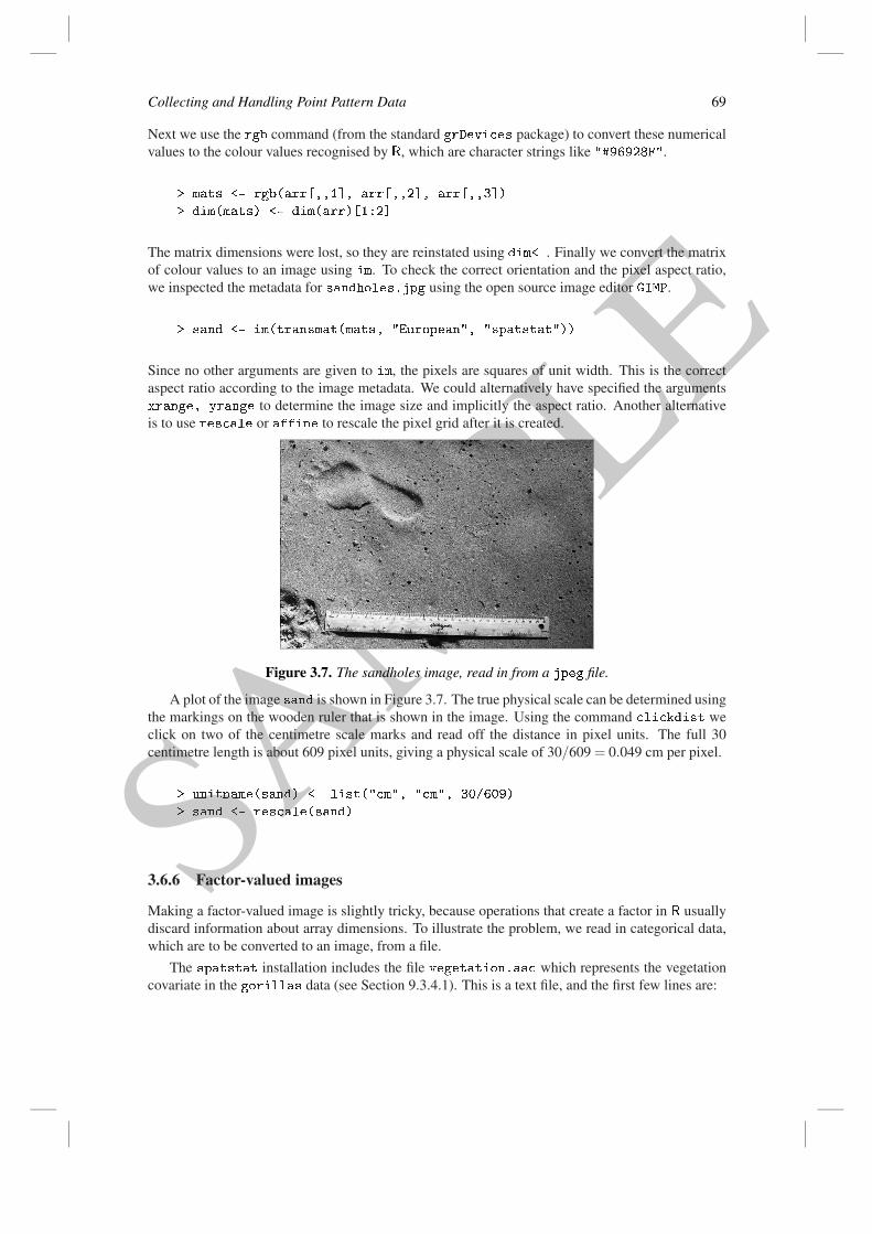
Figure 3.7. The sandholes image, read in from a jpeg file.

A plot of the image sand is shown in Figure 3.7. The true physical scale can be determined usingthe markings on the wooden ruler that is shown in the image. Using the command li kdist weclick on two of the centimetre scale marks and read off the distance in pixel units. The full 30centimetre length is about 609 pixel units, giving a physical scale of 30/609= 0.049 cm per pixel.

> unitname(sand) <- list(" m", " m", 30/609)

> sand <- res ale(sand)

3.6.6 Factor-valued images

Making a factor-valued image is slightly tricky, because operations that create a factor in R usuallydiscard information about array dimensions. To illustrate the problem, we read in categorical data,which are to be converted to an image, from a file.

The spatstat installation includes the file vegetation.as which represents the vegetationcovariate in the gorillas data (see Section 9.3.4.1). This is a text file, and the first few lines are:

SAMPLE


n ols 181

nrows 149

xll orner 580440.38505253

yll orner 674156.51146465

ellsize 30.70932052048

NODATA_value -9999

-9999 -9999 -9999 1 1 1 -9999 -9999 -9999

The file uses a simple format defined by the geospatial library GDAL. It could be read automat-ically using the function readGDAL from the package rgdal. If rgdal is not installed, we cansimply read the body of the data using s an, skipping the first 6 lines of header information:

> fn <- system.file("rawdata", "gorillas", "vegetation.as ",

pa kage="spatstat")

> pixvals <- s an(fn, skip=6)

> pixvals[pixvals == -9999℄ <- NA

> mat <- matrix(pixvals, nrow=149, n ol=181, byrow=TRUE)

Note the use of byrow=TRUE because the rows of the data file are horizontal rows of pixels.The entries in the matrix mat are the digits 1 to 6 corresponding to the following vegetation

types:

> vtype <- ("Disturbed", "Colonising", "Grassland",

"Primary", "Se ondary", "Transition")

We convert mat to a factor:

> f <- fa tor(mat, labels=vtype)

> is.fa tor(f)

[1℄ TRUE

> is.matrix(f)

[1℄ FALSE

Although mat was a matrix, f is not. It is a factor, with no array dimensions. However, one canassign a dim attribute to a factor:

> dim(f) <- (149,181)

It is then possible to convert the factor to a pixel image:

> fa torim <- im(f)

By default the pixels have unit size. We would usually want to specify the correct spatial coordi-nates, given in the header above.

> x0 <- 580440.38505253 ; y0 <- 674156.51146465

> dx <- dy <- 30.70932052048

> fa torim <- im(f, xrange=x0 + dx * (0, 181),

yrange=y0 + dy * (0, 149))

Alternatively we could have specified the arguments x ol, yrow giving the coordinates of eachrow and column of pixels. The image fa torim is plotted in Figure 3.8.

A third alternative is to create an integer-valued matrix, and assign a levels attribute to it. Thiswill be interpreted as a matrix with categorical values.

SAMPLE


Disturbed

Colonising

Grassland

Primary

Secondary

Transition

Figure 3.8. The image fa torim created in the text.

3.6.7 Computed images

Many functions in spatstat return a pixel image. These include pixellate and as.im (whichperform discretisation), density.ppp, density.psp, blur, Smooth, relrisk (kernel smooth-ing), adaptive.density (nonlinear smoothing), Smooth, idw, nnmark (interpolation), distmap,nnmap (distance functions), predi t.ppm, predi t.kppm, intensity.ppm (model prediction),and rnoise (which generates random pixel noise).

3.6.8 Images from functions

Amathematical function (described by an explicit formula) may be converted to a pixel image usingas.im.

> f <- fun tion(x,y){15*( os(sqrt((x-3)^2+3*(y-3)^2)))^2}

> A <- as.im(f, W=square(6))

The image A is plotted in Figure 3.9. Note the mandatory observation window argument W; an imageis always confined to a spatial region, which in this case must be given by the user, since it cannotbe inferred from a function. Additional arguments to as.im control the pixel resolution.

3.6.9 Alternative to images: spatial function class "funxy"

Converting a function to a pixel image involves discretisation, which may be undesirable in somecircumstances. An alternative to discretising the function f above would have been to register it asa ‘spatial function’:

> g <- funxy(f, W=square(6))

The result g is a copy of f with extra attributes, including the specified window W, and belongs tothe special class "funxy". This object can be used in many places where a pixel image is expected.It behaves like a pixel image in many ways, except that it is able to calculate the function valueexactly at any spatial location.

SAMPLE


0

2

4

6

8

10

12

14

Figure 3.9. A function converted to a pixel image.

In a "funxy" object, computation of the function values is deferred until the last possible mo-ment, that is, until g(x,y) is evaluated for coordinates x,y. In a pixel image the pixel values havealready been computed when we create the image object.

3.7 Line segment patterns

Spatial data often include linear features such as roads, rivers, and geological faults. For example,the Queensland copper data shown in Figure 1.11 consist of a point pattern of known copper depositsand a spatial pattern of linear geological features, mostly faults, observed at the surface. A patternof straight line segments can be stored in the spatstat package as an object of class "psp" (forplanar segment pattern).

Many functions are available for creating and manipulating "psp" objects. To create a "psp"object use psp or as.psp. The creator function psp requires vectors x0, y0, x1, and y1 specifyingthe endpoints of the segments, and a window (object of class "owin") in which the segments wereobserved. The conversion function as.psp allows the user to specify line segments in other ways,for example by specifying their midpoint, length, and orientation.

Random patterns of line segments may be created by randomly generating the vectors of end-points (using psp), or randomly generating the midpoints, lengths, and orientations (using as.psp).A random line segment pattern from the Poisson line process may be generated using the functionrpoisline. The infinite lines are clipped to the given window resulting in a pattern of segments.

The boundary edges of a window can be extracted as a "psp" object using the edges function.

Like planar point patterns, "psp" objects may be marked by a vector or data frame. The genericfunctions provided in spatstat for assigning, interrogating, and manipulating marks all have meth-ods for the "psp" class.

See Section 4.4 for information on how to manipulate line segment patterns. Table 4.17 listsfunctions for extracting information from "psp" objects. Additionally Table 4.6 lists generic func-tions for performing geometric operations on spatial objects, including objects of class "psp".

SAMPLE


3.8 Collections of objects

3.8.1 The "solist" and "anylist" classes

In spatial statistics it is often necessary to handle a collection of several objects, such as a collectionof point patterns. In the R language, a collection of things is usually organised as a list. Thespatstat package supports two special classes of lists, "solist" and "anylist".

A solist object (spatial object list) is a list of ‘spatial’ objects in two dimensions. An ob-ject is recognised as ‘spatial’ if it occupies a definite region in two-dimensional space; examplesinclude "owin", "ppp", "psp", "im", "ppm" and "layered" objects. In spatstat we use asolist object to store several different spatial objects of the same class, for example, several pointpatterns, or to store the results of several transformations applied to the same spatial dataset. Thewaterstriders dataset (Figure 1.2) is a "solist" object, essentially a list of three point patterns.

A "solist" object can be created explicitly by solist(entry1, entry2, ...) or byas.solist(xxx) where xxx is a list of (spatial) objects. For example:

> P <- solist(A= ells, B=japanesepines, C=redwood)

Various functions in spatstat produce objects of class "solist". There are numerous methodsfor the "solist" class, most notably a plot method (Section 4.1.6.2). The list P could be plottedimmediately by plot(P) and this would display the three point patterns side by side.

An anylist object is a list of objects of a very general kind (not necessarily spatial objects)that we intend to treat in a similar way. One can, for example, use an anylist object to store theresults of the same statistical technique applied to different spatial datasets, or the results of severaldifferent types of analysis applied to the same spatial dataset. For example the estimates of Ripley’sK-function (Chapter 7) for each of the point patterns in the list P could be stored as

> KP <- anylist(A=Kest( ells), B=Kest(japanesepines), C=Kest(redwood))

or equivalently

> KP <- as.anylist(lapply(P, Kest))

There is also a plot method for "anylist" objects, which is only appropriate if each of the listentries can be plotted by its own plot method (see Section 4.1.6.2). The list KP could be plottedimmediately by plot(KP) and would show the three K-functions side by side.

3.8.2 The "hyperframe" class

Another important class for storing collections of objects is the "hyperframe" class. A hyperframeis an array, ‘like a data frame’, but more general. Hyperframes allow the entries of columns to beobjects of any class. The only constraint is that all the entries in a particular column must be of thesame kind.

A hyperframe can be used to store the results of an experiment in which several point patternswere observed. One column of the hyperframe contains the observed point patterns, and othercolumns may contain covariate data. The point patterns may have been observed under identicalconditions (replicated point patterns) or under different experimental conditions indicated by thecovariates.

For example, the waterstriders dataset is a list of three point patterns obtained under identicalconditions. It can be converted to a hyperframe with one column:

> ws <- hyperframe(Larvae=waterstriders)

SAMPLE


Additional columns can be added in the same way as for a data frame.

Hyperframes are covered in Chapter 16, in particular Section 16.4. They appear again briefly inSection 3.10.3.6 below.

3.9 Interactive data entry in spatstat

Spatial data can also be entered interactively, using a graphical point-and-click interface. The facil-ities are listed in Table 3.3. They are rudimentary compared to other specialised graphics packages,but they have the advantage that the data will immediately be entered in a spatstat data format.The interface is robust and available on almost any computer platform, since it depends only on thebase R graphics system.

FUNCTION RESULT

li kppp point pattern li kbox rectangle li kpoly polygonal window li kdist measured distance li kjoin adjacency matrix for linear network

Table 3.3. Interactive data entry facilities in spatstat.

These facilities are useful for rapid experimentation and exploration, and for annotating otherkinds of spatial data. To ‘annotate’ spatial data, we display the original data, and use the graphicalinterface to superimpose new spatial information such as points, lines, or text. For these tasks itis recommended that RStudio users open the system’s native R graphics device as explained inSection 2.1.11.

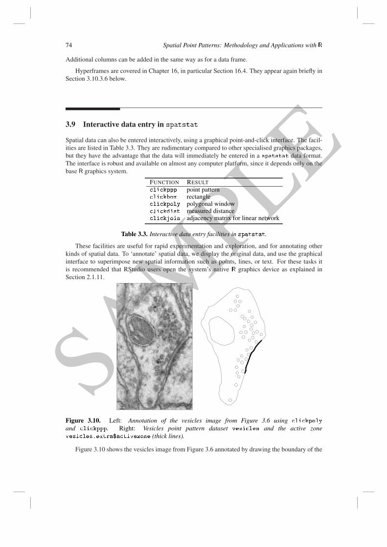
Figure 3.10. Left: Annotation of the vesicles image from Figure 3.6 using li kpoly

and li kppp. Right: Vesicles point pattern dataset vesi les and the active zone

vesi les.extra$a tivezone (thick lines).

Figure 3.10 shows the vesicles image from Figure 3.6 annotated by drawing the boundary of the

SAMPLE


mitochondrial region with li kpoly and marking the locations of some of the synaptic vesicleswith li kppp:

> plot(vim)

> mito <- li kpoly(add=TRUE, ol="white", win=Window(vim))

> vesi <- li kppp(add=TRUE, ol="white", win=Window(vim))

Tracing the mitochondrial boundary is relatively easy because of the strong contrast. The vesicleshave weaker contrast and fewer contextual cues, so they are more difficult to recognise withoutbiological training and experience. In microscopy, each experimental protocol includes standardisedcriteria for recognising and counting the microstructures of interest. The vesi les point patterninstalled in spatstat was annotated by a trained microscopist using such a protocol. It is aninteresting exercise to compare your own guesses with the expert’s annotation by typing

> plot(vesi les, add=TRUE, hars=3, ol="green")

If that is too difficult, try annotating the sandholes image (Figure 3.7). Remember that .Last.valuecan also be used to capture the result of the last command.

For accurate annotation, it would be better to use specialised software from the field of applica-tion.

3.10 Reading GIS file formats

3.10.1 GIS file formats

Many different file formats are used to store spatial data for use in Geographical Information Sys-tems (GIS) and other applications. Common formats include shapefiles, NetCDF, and GRIB.

Typically spatstat does not support these formats directly: this would not be good softwaredesign. Instead, we rely on specialised R packages which exist for handling different spatial datafile formats. Table 3.4 lists some useful packages.

maptools Tools for reading and handling spatial objectsshapefiles Read and write ESRI™ shapefilesRAr Info interface to ArcInfo system and data formatrgdal interface to GDAL geographical data analysis systemGeoXp interactive spatial exploratory data analysissp spatial data classes and methods

Table 3.4. Packages for handling GIS data files.

For our purposes the most useful file-handling package is maptools. It recognises a largenumber of different file formats, and contains interface code for exchanging spatial objects betweendifferent R packages.

When a file is read by maptools, the data are represented in R using the data structures definedin the package sp. The sp package [111] supports a standard set of spatial data types in R. Thesestandard data types can be handled by many other packages, so it is useful to convert your spatialdata into one of the data types supported by sp.

The maptools package also contains code for converting sp data types to the data structuressupported by spatstat. Our recommended strategy for converting spatial data from a standardGIS format into spatstat is: (1) using the facilities of maptools, read the data and store the data

SAMPLE


in one of the standard formats supported by sp; (2) convert the sp data type into one of the datatypes supported by spatstat, typically using maptools.

Using the sp data types as an intermediate stage is also useful if you plan to employ other Rpackages for spatial data analysis, which often use the sp data types.

3.10.2 Read shapefiles using maptools

A shapefile [254] represents a list of spatial objects— a list of points, a list of lines, or a list of polyg-onal regions — and each object in the list may have additional variables attached to it. A datasetstored in shapefile format is actually stored in a collection of text files, for example baltim.shp,baltim.prj, baltim.sbn, baltim.dbf, which all have the same base name baltim but differentfile extensions. To refer to this collection, always use the file name with the extension shp.

The maptools package contains facilities for reading and writing files in shapefile format. Aspatial dataset is read in to R using x <- readShapeSpatial("filename.shp"). The class ofthe resulting object xmay be "SpatialPoints" indicating a point pattern, "SpatialLines" indi-cating a list of polygonal lines, or "SpatialPolygons" indicating a list of polygons. It may also be"SpatialPointsDataFrame", "SpatialLinesDataFrame", or "SpatialPolygonsDataFrame"indicating that, in addition to the spatial objects, there is a data frame of additional variables.The classes "SpatialPixelsDataFrame" and "SpatialGridDataFrame" represent pixel imagedata.

Here are some examples, using the example shapefiles supplied in the maptools package itself.

> library(maptools)

> oldfolder <- getwd()

> setwd(system.file("shapes", pa kage="maptools"))

> baltim <- readShapeSpatial("baltim.shp")

> olumbus <- readShapeSpatial(" olumbus.shp")

> fylk <- readShapeSpatial("fylk-val.shp")

> setwd(oldfolder)

Then lass(baltim) returns "SpatialPointsDataFrame", while lass( olumbus) returns"SpatialPolygonsDataFrame" and lass(fylk) returns "SpatialLinesDataFrame".

3.10.3 Converting sp data to spatstat format

To convert a dataset in sp format to an object in the spatstat package, the subsequent proceduredepends on the type of data, as explained below.

3.10.3.1 Objects of class "SpatialPoints"

An object x of class "SpatialPoints" represents a spatial point pattern. Use as(x, "ppp") oras.ppp(x) to convert it to a spatial point pattern in spatstat.

The window for the point pattern will initially be taken from the bounding box of the points.You will probably wish to change this window, usually by taking another dataset to provide thewindow information. Use [.ppp to change the window: if X is a point pattern object of class "ppp"and W is a window object of class "owin", type X <- X[W℄.

3.10.3.2 Objects of class "SpatialPointsDataFrame"

An object x of class "SpatialPointsDataFrame" represents a pattern of points with additionalvariables attached to each point. It includes an object of class "SpatialPoints" giving the pointlocations, and a data frame containing the additional variables attached to the points.

SAMPLE


Use y <- as(x, "ppp") or y <- as.ppp(x) to convert a "SpatialPointsDataFrame"

object x to a spatial point pattern y in spatstat. In this conversion, the data frame of additionalvariables in x will become the marks of the point pattern z. Before the conversion you can ex-tract the data frame of auxiliary data by df <- x�data or df <- slot(x, "data"). After theconversion you can extract these data by df <- marks(y). For example:

> balt <- as(baltim, "ppp")

> bdata <- slot(baltim, "data")

3.10.3.3 Objects of class "SpatialLines"

A ‘line segment’ is the straight line between two points in the plane. In the spatstat package, anobject of class "psp" (‘planar segment pattern’) represents a pattern of line segments, which mayor may not be connected to each other (like matches which have fallen at random on the ground). Inthe sp package, an object of class "SpatialLines" represents a list of lists of connected curves,each curve consisting of a sequence of straight line segments that are joined together (like severalpieces of a broken bicycle chain). These two data types do not correspond exactly: see Figure 3.11.

Figure 3.11. Objects of class "psp" (Left) and "SpatialLines" (Right).

The list-of-lists hierarchy in a "SpatialLines" object is useful when representing internaldivisions in a country. For example, if USA is an object of class "SpatialLines" representingthe borders of the United States of America, then USA�lines might be a list of length 51, withUSA�lines[[i℄℄ representing the borders of the i-th State. The borders of each State consist ofseveral different curved lines. Thus USA�lines[[i℄℄�Lines[[j℄℄ would represent the jth pieceof the boundary of the i-th State.

If x is an object of class "SpatialLines", there are at least two different ways to convert xto a spatstat object. The first is to collect together all the line segments that make up all theconnected curves and store them as a single object of class "psp". To do this, use as(x, "psp")

or as.psp(x) to convert x to a spatial line segment pattern. The window for the line segmentpattern can be specified as an argument window to as.psp.

The second way is to convert each connected curve to an object of class "psp", keeping differentconnected curves separate. To do this, type f <- fun tion(z){ lapply(z�Lines, as.psp) }

and out <- lapply(x�lines, f). The result will be a list of lists of objects of class "psp".Each one of these objects represents a connected curve, although the spatstat package does notknow that. The list structure will reflect the list structure of the original "SpatialLines" objectx. If that is not desired, then collapse the list-of-lists-of-"psp"’s into a list-of-"psp"’s using one ofthese two commands:

urvelist <- do. all(" ", out)

urvegroup <- lapply(out, fun tion(z) { do. all("superimposePSP", z)})

In the first case, urvelist[[i℄℄ is a "psp" object representing the i-th connected curve. In thesecond case, urvegroup[[i℄℄ is a "psp" object containing all the line segments in the i-th groupof connected curves (for example the i-th State in the USA example).

SAMPLE


3.10.3.4 Objects of class "SpatialLinesDataFrame"

An object x of class "SpatialLinesDataFrame" is a "SpatialLines" object with additionaldata. The additional data are stored as a data frame x�datawith one row for each entry in x�lines,that is, one row for each group of connected curves.

In the spatstat package, an object of class "psp" may have a data frame of marks. Note thateach individual line segment in a "psp" object may have different mark values.

If x is an object of class "SpatialLinesDataFrame", it can be converted to a single object ofclass "psp" using y <- as(x, "psp") or y <- as.psp(x). The mark variables attached to aparticular group of connected lines in x will be duplicated and attached to each line segment in theresulting "psp" object y.

Alternatively x can be converted to a list of lists of "psp" objects as follows:

out <- lapply(x�lines, fun tion(z) { lapply(z�Lines, as.psp) })

dat <- x�data

for(i in seq(nrow(dat)))

out[[i℄℄ <- lapply(out[[i℄℄, "marks<-", value=dat[i, , drop=FALSE℄)

See the previous subsection for explanation on how to change this using or superimposePSP.

3.10.3.5 Objects of class "SpatialPolygons"

First some terminology. A polygon is a closed curve that is composed of straight line segments. Youcan draw a polygon without lifting your pen from the paper. A polygonal region is a region in spacewhose boundary is composed of straight line segments. A polygonal region may consist of severalunconnected pieces, and each piece may have holes. The boundary of a polygonal region consistsof one or more polygons. To draw the boundary of a polygonal region, you may need to lift anddrop the pen several times. See Figure 3.12.

Figure 3.12. Distinction between a polygon (Left) and a polygonal region (Right).

An object of class "owin" in spatstat, if it is polygonal, represents a single polygonal region.It is a region of space that is delimited by boundaries made of lines. It may consist of severaldisconnected pieces, and may have holes.

An object x of class "SpatialPolygons" represents a list of polygons. For example, a singleobject of class "SpatialPolygons" could store information about every State in the United Statesof America (or the United States of Malaysia). Each State would be a separate polygonal region(and it might contain holes such as lakes).

SAMPLE


There are two different ways to convert an object of class "SpatialPolygons". The first isto combine all the polygonal regions together into a single polygonal region, and convert this to asingle object of class "owin". For example, we could combine all the States of the USA togetherand obtain a single object that represents the territory of the USA. To do this, use as(x, "owin")

or as.owin(x). The result is a single window (object of class "owin") in the spatstat package.The second way is to keep the different polygonal regions separate, and convert each one of the

polygonal regions to an object of class "owin". For example, we could keep the States of the USAseparate, and convert each State to an object of class "owin". To do this, type the following:

regions <- slot(x, "polygons")

regions <- lapply(regions,

fun tion(x) { SpatialPolygons(list(x)) })

windows <- solapply(regions, as.owin)

The result is a list of objects of class "owin". Often it would make sense to convert this to atessellation object, by typing te <- tess(tiles=windows).

During the conversion process, the geometry of the polygons will be automatically ‘repaired’if needed. Polygon data from shapefiles often contain geometrical inconsistencies such as self-intersecting boundaries and overlapping pieces. For example, these can arise from small errors incurve-tracing. Geometrical inconsistencies are tolerated in an object of class "SpatialPolygons"which is a list of lists of polygonal curves. However, they are not tolerated in an object of class"owin", because an "owin"must specify a well-defined region of space. These data inconsistenciesmust be repaired to prevent technical problems. The spatstat package uses polygon-clipping codeto automatically convert polygonal lines into valid polygon boundaries. The repair process changesthe number of vertices in each polygon, and the number of polygons (if you chose option 1 above).To disable the repair process, set spatstat.options(fixpolygons=FALSE).

3.10.3.6 Objects of class "SpatialPolygonsDataFrame"

An object x of class "SpatialPolygonsDataFrame" represents a list of polygonal regions, withadditional variables attached to each region. It includes an object of class "SpatialPolygons"giving the spatial regions, and a data frame containing the additional variables attached to the re-gions. The regions are extracted by y <- as(x, "SpatialPolygons") and we then proceed asabove to convert the curves to spatstat format.

The data frame of auxiliary data is extracted by df <- x�data or df <- slot(x, "data").For example:

> p <- as( olumbus, "SpatialPolygons")

> regions <- slot( p, "polygons")

> regions <- lapply( regions, fun tion(x){ SpatialPolygons(list(x)) })

> windows <- solapply( regions, as.owin)

There is currently no facility in spatstat for attaching additional variables to an "owin" objectdirectly. Marks can be attached to the tiles of a tessellation. Alternatively we can make use of the"hyperframe" class described in Section 3.8.2:

> h <- hyperframe(window= windows)

> h <- bind.hyperframe( h, olumbus�data)

The resulting object h is a hyperframe containing a column of "owin" objects followed by thecolumns of auxiliary data.

SAMPLE


3.10.3.7 Objects of class "SpatialGridDataFrame" and "SpatialPixelsDataFrame"

An object x of class "SpatialGridDataFrame" represents a pixel image on a rectangular grid. Itincludes a "SpatialGrid" object slot(x, "grid") defining the full rectangular grid of pixels,and a data frame slot(x, "data") containing the pixel values (which may include NA values).

The command as(x, "im") converts x to a pixel image of class "im", taking the pixel val-ues from the first column of the data frame. If the data frame has multiple columns, these wouldcurrently have to be converted to separate pixel images in spatstat. For example

y <- as(x, "im")

ylist <- lapply(slot(x, "data"), fun tion(z, y) { y[,℄ <- z; y }, y=y)

An object x of class "SpatialPixelsDataFrame" represents a subset of a pixel image. To convertthis to a spatstat object, it should first be converted to a "SpatialGridDataFrame" by as(x,

"SpatialGridDataFrame"), then handled as described above.

3.11 FAQ

• Why doesn’t spatstat use the same classes as sp?

Development of spatstat started long before sp. The data types in spatstat and sp are basedon different abstractions and are not completely interchangeable, as explained in Section 3.10.The spatstat package uses S3 method dispatch while sp uses S4 classes and methods.

• Can/should I record points lying just outside the sampling quadrat?

Yes, this can be done. Point pattern objects created with ppp can include such points (as ‘rejects’).Of course this implies that you are not simply observing the point pattern through a ‘window’, andthe sampling procedure is somewhat unclear (what rule exactly was applied to decide whether apoint is recorded?). The presence of such points changes the treatment of edge effects. Manyfunctions in spatstat can handle such data by setting the argument domain or subset to equalthe sampling quadrat.

• How can I include French or Scandinavian accents, Greek characters, or Maori language dia-

critical marks in the name of the unit of length, a factor level, an axis label, or the legend of a

plot?

Find the Unicode number for the desired character in the data frame tools::Adobe_glyphs.Prefix this number by \u to include it in a character string. For example, to find the Greek letterµ :

> df <- tools::Adobe_glyphs

> ii <- mat h("mu", df$adobe)

> df[ii,℄

adobe uni ode

2621 mu 00B5

If X is a point pattern and we assign

> unitname(X) <- "\u00B5m"

then the unit of length will be rendered as "µm" in spatstat’s printed output and graphics (pro-vided the system recognises Unicode). Similarly Ångström (Å) is \u212B. To match all glyphnames that include the string ma ron, use grep("ma ron", df$adobe).

collecting and handling point pattern data ebook.spatstat.org/sample-chapters/chapter03.pdf · e...

Documents