Intelligent Control and Automation, 2017, 8, 44-65 http://www.scirp.org/journal/ica

ISSN Online: 2153-0661 ISSN Print: 2153-0653

DOI: 10.4236/ica.2017.81004 February 24, 2017

Cognitive Supervisor for an Autonomous Swarm of Robots

Vladimir G. Ivancevic, Darryn J. Reid

Decision Sciences, Joint and Operations Analysis Division, Defence Science & Technology Group, Canberra, Australia

Abstract As a sequel to our recent work [1], in which a control framework was devel-oped for large-scale joint swarms of unmanned ground (UGV) and aerial (UAV) vehicles, the present paper proposes cognitive and meta-cognitive su-pervisor models for this kind of distributed robotic system. The cognitive su-pervisor model is a formalization of the recently Nobel-awarded research in brain science on mammalian and human path integration and navigation, performed by the hippocampus. This is formalized here as an adaptive Ha-miltonian path integral, and efficiently simulated for implementation on ro-botic vehicles as a pair of coupled nonlinear Schrödinger equations. The me-ta-cognitive supervisor model is a modal logic of actions and plans that hinges on a weak causality relation that specifies when atoms may change their values without specifying that they must change. This relatively simple logic is de-cidable yet sufficiently expressive to support the level of inference needed in our application. The atoms and action primitives of the logic framework also provide a straightforward way of connecting the meta-cognitive supervisor with the cognitive supervisor, with other modules, and to the meta-cognitive supervisors of other robotic platforms in the swarm.

Keywords Autonomous Robotic Swarm, Cognitive Supervisor, Hippocampus Path Integration and Navigation, Hamiltonian Path Integral, Modal Logic, Nonlinear Schrödinger Equation, Reasoning about Actions and Plans

1. Introduction

Recently, we have proposed in [1] a rigorous model for prediction and control of a large-scale joint swarm of unmanned ground vehicles (UGVs) and unmanned aerial vehicles (UAVs), performing an autonomous land-air operation. In that paper, we have also introduced a need for a cognitive supervisor for the high-

How to cite this paper: Ivancevic, V.G. and Reid, D.J. (2017) Cognitive Supervisor for an Autonomous Swarm of Robots. Intelligent Control and Automation, 8, 44- 65. https://doi.org/10.4236/ica.2017.81004 Received: January 16, 2017 Accepted: February 21, 2017 Published: February 24, 2017 Copyright © 2017 by authors and Scientific Research Publishing Inc. This work is licensed under the Creative Commons Attribution International License (CC BY 4.0). http://creativecommons.org/licenses/by/4.0/

Open Access

V. G. Ivancevic, D. J. Reid

45

dimensional distributed multi-robotic system. Its primary task is to have a birds- eye view of the situation across the joint land-air operation, and based on the GPS locations of both the target and all included robots, to provide them with good 2D and 3D attractor fields so that they can reach the proximity of the tar-get in the shortest possible time. The purpose of the present paper is to develop a rigorous model for this cognitive supervisor, based on recent discoveries in brain science that show us how humans navigate in 2D environments and how bats navigate in 3D environments, and to couple this with a meta-cognitive supervi-sor model that allows vehicles to reason about actions and construct simple plans.

The 2014 Nobel Prize in Physiology or Medicine was awarded jointly to John O’Keefe, May-Britt Moser and Edvard I. Moser “for their discoveries of cells that constitute a positioning system in the brain’’, in other words, for the hippo- campus path integration and navigation system.

Briefly, there is a part of a mammal brain, called the hippocampal formation, which in humans is mostly developed in taxi drivers, grows in size with their experience and can be also trained (like a muscle) using fast-action video games. The hippocampal formation provides a cognitive map of a familiar environment which can be used to identify one’s current location and to navigate from one place to another. This mapping system provides two independent strategies for locating places, one based on environmental landmarks and the other on a path integration system (see [2] [3] and the references therein), which uses informa-tion about distances traveled in particular directions. This brain navigation sys-tem exists in all mammals, while in humans it additionally provides the basis for the so-called episodic memory [4].1

Two main components of the hippocampal formation (discovered by O’Keefe) are: (i) hippocampal place cells, and (ii) grid cells from the entorhinal cortex (discovered by Mosers). In particular, according to Edvard Moser, “All network models for grid cells involve continuous attractors ...”—which is similar to our attractor Hamiltonian dynamics of UGVs and UAVs, given by Equations (1)-(2) in the next section.

As inspired by this discovery in brain science, the present paper proposes a novel probabilistic spatio-temporal model for mammalian path integration and navigation, formulated as an adaptive Hamiltonian path integral. The model combines: (i) a cognitive map ( )p t performed by hippocampal place cells, (ii) an entorhinal map ( )q t performed by grid cells, (iii) a current of sensory (ex-tra-hippocampal) stimuli ( )J t , and (iv) Hebbian learning in hippocampal synaptic weights ( )w t . This model represents an infinite-dimensional neural network, which can be simulated (using 106 - 107 neurons) on IBM’s TrueNorth chip.

We also propose to couple this cognitive supervisor to a meta-cognitive su-pervisor, supporting dynamic mission planning, using on an established pro- positional multimodal logic framework. This approach gives robotic vehicles the

1For technical details on the Nobel awarded work of John O’Keefe, May-Britt Moser and Edvard I. Moser, see Appendix and the references therein.

V. G. Ivancevic, D. J. Reid

46

ability to construct and execute simple plans on the fly against goals, given local sensor information, state information communicated locally between vehicles, and aspects of the state of the robot itself. The coupling to the cognitive supervi-sor and to the outside world is through the truth value of logical atoms and us-ing multimodal actions.

2. Affine Hamiltonian Control for a Joint (UGV + UAV) Swarm

The affine Hamiltonian control model with many degrees-of-freedom has been presented in the form of 2n-dimensional (2ND) Langevin-type attractor matrix equations with nearest-neighbor couplings, which represent two recurrent neur-al networks:

UGV-swarm:

( ) ( )

( ) ( )

2 2 2

,

2 2 2

,

,

.

D Djk A jk jk jk jk p jk jk qjk

j k

D Djk A jk jk jk jk q jk jk pjk

j k

q q q q p H u t

p p p p q H u t

ϕ ω η

ϕ ω η

= − − − ∂ +

= − − + ∂ +

∑

∑

(1)

UAV-swarm:

( ) ( )

( ) ( )

3 3 2

, ,

3 3 2

, ,

,

.

D Djkl A jkl jkl jkl jkl p jkl jkl qjkl

j k l

D Djkl A jkl jkl jkl jkl q jkl jkl pjkl

j k l

q q q q p H u t

p p p p q H u t

ϕ ω η

ϕ ω η

= − − − ∂ +

= − − + ∂ +

∑

∑

(2)

The following terms are used in Equations (1) and (2): ( )jk jkq q t= and ( )jk jkp p t= are time-evolving matrices defining coordinates and momenta of

the UGV-swarm, respectively, with initial conditions: ( )0jkq and ( )0jkp . Si-milarly, ( )jkl jklq q t= and ( )jkl jklp p t= are time-evolving tensors defining coordinates and momenta of the UAV-swarm, respectively, with initial condi-tions: ( )0jklq and ( )0jklp . 2D

Aq and 2DAp are the 2D attractors for the UGV

swarm, while 3DAq and 3D

Ap are the 3D attractors for the UGV swarm. 2Dϕ and 3Dϕ are the attractor field strengths for the UGV and UAV swarms, re-spectively; jkω and jklω are corresponding adaptive weights of both swarms which can be trained by Hebbian learning, ( ),jk jkq p and ( ),jkl jklq p are the initial formations of both swarms, jku and jklu are Lie-derivative controllers for both swarms, jkH and jklH are affine Hamiltonians of both swarms, while

( )q tη and ( )p tη are zero-mean, delta-correlated, Gaussian white noises add-ed to q and p variables in both swarms. For more technical details on affine Hamiltonian (or, similar, port-Hamiltonian) control of large-scale dynamical systems, see [1] and the references therein.

The purpose of the cognitive supervisor is to provide the 2D and 3D inputs to the recurrent neural nets (1)-(2), or specifically, 2D attractors ( )2 2,D D

A Aq p for the UGV-swarm and 3D attractors ( )3 3,D D

A Aq p for the UAV-swarm (see, e.g. [5]).

3. Adaptive Hamiltonian Path Integral

In his recent Nobel lecture, John O’Keefe referred to his pioneering 1976-paper [6] [7], describing the function of the hippocampal place cells performing Tol-man’s cognitive mapping: “When an animal had located itself in an environment

V. G. Ivancevic, D. J. Reid

47

(using environmental stimuli) the hippocampus could calculate subsequent po-sitions in that environment on the basis of how far and in what direction the animal had moved in the interim ...” This quotation was accompanied by a commutative diagram depicting the vector addition and a suggestion that an animal moves in a sequence of vectors.

This extract from O’Keefe’s lecture is the motivation for the present mathe-matical model. Basically, any two-dimensional (2D) vector is equivalent to a complex number: i ,z x y= + where ( ,x y ) are Cartesian coordinates and i 1.= − The same complex number z can be also given in the polar form as:

iez r θ= , where r is the radius vector and θ is the heading. The sequence of N vectors is the sum of complex numbers:

i

1 1 1particle likeanimalmotion i e .

N N Nk

k k k kk k k

z x y r θ

= = =

− = = + =∑ ∑ ∑ (3)

In this way, we can describe a particle-like animal motion in the complex plane , from some initial point A to the final point ,B performed in N steps, as an integral complex number (3). This basic idea describes an animal’s motion in purely static and deterministic terms; it can be generalized into a more realistic, probabilistic dynamics, as follows.2

Now, instead of the complex plane , consider a particle-like animal motion in the phase plane (p-q), where ( ),p p t x= represents the action of the hippo-campal place cells and ( ),q q t x= defines the action of the entorhinal grid cells. The animal moves from some initial point A given by canonical coordinates ( 0 0, q p ) at initial time 0t , to the final point B given by canonical coordinate ( 1 1, q p ) at final time 1t , via all possible paths, each path having an equal probability (so that the sum of all path-probabilities is = 1). This most general 2D motion is properly defined by the transition amplitude:

1 1 1 0 0 0, , , ,B A q p t q p t≡

whose absolute square represents the transition probability density function: 2 2

1 1 1 0 0 0, , , , .PDF B A q p t q p t= ≡

The transition amplitude B A can be calculated via the following Hamil-tonian path integral3

2For For simplicity reasons, we are using the same Hamiltonian symbols, q and p , for the cogni-tive representation of robotic coordinates and momenta, to emphasize the one-to-one correspon-dence between the physical robotic level and the mental supervisor level. However, while at the physical robotic level, ( )q q t= and ( )p p t= are only temporal variables, at the cognitive level,

( ),q q t x= and ( ),p p t x= represent spatiotemporal wave functions. 3The path integral (4) was formulated by R. Feynman in [10]. It has been widely appreciated that the phase-space (i.e., Hamiltonian) path integral is more generally applicable, or more robust, than the original, Lagrangian version of the path integral, introduced in Feynman’s first paper [11]. For ex-ample, the original Lagrangian path integral is satisfactory for Lagrangians of the form:

( ) ( ) ( )21 ,2

L x mx A x x V x= + − but it is unsuitable, e.g., for the case of a particle with the Lagrangian

(in normal units): ( ) 21 .L x mqrt x= − − For such a system (as well as many more general expres-

sions) the Hamiltonian path integral is more robust; e.g., the Hamiltonian path integral for the free

particle: [ ] [ ] { }2 2exp i dp q pq qrtp m t− + ∫ ∫ is readily evaluated.

V. G. Ivancevic, D. J. Reid

48

[ ] [ ] ( ) ( ) ( ){ }[ ] [ ] ( ) ( )

1

01 1 1 0 0 0, , , , exp i , d ,

1with d d ,2π

t

tq p t q p t q p p q H p q

q p q pτ

τ τ τ

τ τ

= −

≡

∫ ∫

∏∫ ∫

(4)

where the integration is performed over the ( )p τ and ( )q τ values at every

time ,τ with the time-step 1d j jt tτ −≡ − and the velocity ( )( ) ( )1

1

.j j

j j

q t q tq

t tτ −

−

−≡

−

For technical details of the derivation of the Hamiltonian path integral (4), see e.g. [8] [9] and the references therein.

Next, the sources from various extra-hippocampal stimuli can be incorporated into the basic transition amplitude (4) by adding some form of a bio-electric current J , as:

[ ] [ ] [ ] ( ) ( ) ( ) ( ) ( ){ }1

0exp i , d ,

t

tZ J q p p q H p q J qτ τ τ τ τ= − + ∫ ∫ (5)

where [ ] 1 1 1 0 0 0, , , ,Z J q p t q p t= is the system’s partition function dependent on the current J and obeying the normalization condition: [ ]0 1Z J = = .

A generalization from a single particle Hamiltonian path integral (4) to the probabilistic dynamics of an N-particle system is straightforward. The phase- space functional integral that defines the transition amplitude

1 1 1 1 0 01 1 1 1 0 0 1 0, , , ,N N

N Nq q p p t q q p p t , from the initial ND point ( )10 0

Nq q

at time 0t to the final ND point ( )11 1

Nq q at time 1t is given by:

[ ] [ ] ( ) ( ) ( )

[ ] [ ]

1

0

1 1 1 1 0 01 1 1 1 0 0 1 0

1

1

, , , ,

exp i , d ,

1with d d ,2π

N NN N

Nt k kk kt

k

Nk

kk

q q p p t q q p p t

q p p q H p q

q p q pτ

τ τ τ=

=

= −

=

∑∫ ∫

∏∏∫ ∫

where we are allowing for the full Hamiltonian of the system ( ), kkH p q to de-

pend upon all the N coordinates ( )kq τ and momenta ( )kp τ collectively. Again, we can add various sources as incoming bio-currents kJ as a

straightforward generalization of the single-particle partition function (5) to the system of N particles:

[ ] [ ] [ ] ( ) ( ) ( ) ( ) ( )1

0 1exp i , d ,

Nt k k kN k k k kt

kZ J p q p q H p q J qτ τ τ τ τ

=

= − + ∑∫ ∫

where [ ] 1 1 1 1 0 01 1 1 1 0 0 1 0, , , ,N N

N k N NZ J q q p p t q q p p t= is the system’s par-tition function dependent on all the incoming currents kJ and obeying the normalization condition: [ ]0 1,N kZ J = = for 1, , .k N=

Our final step is to transform the N-particle partition function [ ]N kZ J into an infinite-dimensional recurrent neural network (of a generalized Hopfield type) by including the hippocampal synaptic weights ( )kw τ into it (compare with [12]), as:

V. G. Ivancevic, D. J. Reid

49

[ ]

[ ] [ ] [ ] ( ) ( ) ( ) ( ) ( )

[ ] [ ] [ ]

1

0 1

1

,

exp i , d ,

1with d d d ,2

N k k

Nt k k kk k kt

k

Nk

k kk

Z w J

w q p p q H p q J q

w q p w q pτ

τ τ τ τ τ

π

=

=

= − +

=

∑∫ ∫

∏∏∫ ∫

(6)

where the weights ( )kw τ are adapted (in a discrete time) by Hebbian-type learning:

( ) ( ) ( ) ( )1 ,D Ak k k k

qw w w wτ τ τ τη + = + − (7)

where ( ) ( ), q q τ η η τ= = represent local signal and noise amplitudes, respec-tively, while superscripts D and A denote desired and achieved system states, respectively.

The system (6-7) defines the proposed adaptive Hamiltonian path integral model for a generic mammalian path integration and navigation. Both the se-quential (Ising spin) Hopfield network [13] with its Galuber dynamics and the graded-response Hopfield network [14] with its Fokker-Planck dynamics can be considered as special cases of this general Hamiltonian neural system.

Direct computer simulations of the adaptive Hamiltonian path integral system (6-7) can be performed on the IBM TrueNorth chip (see [15] and the references therein) as a Markov-chain Monte Carlo simulation over a grid of Hopfield nets (which are already implemented in the TrueNorth chip, using 106-107 artificial neurons).

In the next section we propose a more efficient approach to simulate the path integral system (6-7).

4. A Pair of Coupled Nonlinear Schrödinger Equations

In this section, instead of the direct computer simulations on a supercomputer, we will present an indirect approach of simulating the path integral system (6-7) on an ordinary PC, represented as a pair of coupled nonlinear Schrödinger (NLS) equations. In his first paper [11], Feynman showed that his Lagrangian q-path integral was equivalent to the standard linear Schrödinger equation from quan-tum mechanics, given here for the case of a free particle (in natural physical units: 1, 1m= = ):

( ) ( )1i , , , i 1; with ,2t xx zt x t x

zψψ ψ ψ ∂ ∂ = − ∂ = − ∂ = ∂

(8)

which defines the complex-valued microscopic wave function ( ),t xψ ψ= , whose absolute square ( ) 2

,x tψ defines the probability density function (PDF).

In the last decade it was shown (see [16] and the references therein) that if the linear Schrödinger Equation (8) is put into an adaptive (iterative) feedback loop, it adds a cubic nonlinearity with a potential field ( )V V x= and becomes the NLS equation:

21i ,2t xx Vψ ψ ψ ψ∂ = − ∂ + (9)

V. G. Ivancevic, D. J. Reid

50

which now defines the macroscopic wave function ( ),t xψ ψ= whose absolute square ( ) 2

,x tψ still defines the PDF [17]. A variety of analytical solutions for the NLS Equation (9) have been reported in [18] [19].

Finally, to represent the Hamiltonian ( ),q p -path integral, we can use the ( ),q p -pair of NLS equations, as follows.

4.1. Special Case: Analytical Soliton

We start with a simple ( ),q p -NLS pair representation for the path integral sys-tem (6-7), which admits the analytical closed-form solution, given by the so-called Manakov system (with the constant potential V ):4

( )2 21i ,2t xxq q V q p q∂ = − ∂ + + (10)

( )2 21i ,2t xxp p V q p p∂ = − ∂ + + (11)

which was proven in [20], using the Lax pair representation [21], to be com-pletely integrable Hamiltonian system, by the existence of infinite number of involutive integrals of motion.

The ( ),q p -NLS pair (10)-(11) admits both “bright” and “dark” soliton as solutions, of which the simplest one is the so-called Manakov bright 2-soliton given by:

( )( ) ( ) ( )2 22i 2 21

2

,2 sech 2 4 e ,

,a t ax b tq t x c

b b x atp t x c

− + − = +

(12)

where a and b are real-valued parameters and 2 21 2 1.c c+ =

4.2. General Case: Numerical Simulation

Now that we have introduced the simple ( ),q p -NLS pair, we can define our real representation for the path integral system (6-7), as the following more gen-eral ( ),q p -NLS pair:

( ) ( ) ( ) ( ) ( ) ( )21i , , , , , , ,2t k xxq t x w I t x q t x V t x q t x p t x∂ = − ∂ + (13)

( ) ( ) ( ) ( ) ( ) ( )21i , , , , , , ,2t k xxp t x w J t x p t x U t x p t x q t x∂ = − ∂ + (14)

including the bell-shaped (sech) spatiotemporal potentials:

( ) ( ) ( ) ( )3 31 2

1 1, sech , , sech ,2 2

V t x a t x U t x a t x= =

and the soft-step shaped (tanh) spatiotemporal input currents:

( ) ( ) ( ) ( )3 33 4 5 6, tanh , , tanh ,I t x a a t x J t x a a t x= =

together with the common initial condition:

( ) ( )1 1exp i sech ,2 2

x x xχ =

4The Manakov system has been used to describe the interaction between wave packets in dispersive conservative media, and also the interaction between orthogonally polarized components in nonli-near optical fibres (see, e.g. [22] [23] and the references therein).

V. G. Ivancevic, D. J. Reid

51

the set of parameters:

( )1 2 3 4 5 6i 1, 0.4, 0.6, 0.3, 0.8, 0.7, 0.2a a a a a a= − = = = = = =

and the set of adaptive synaptic weights .kw The ( ),q p -NLS pair (13)-(14) has been numerically simulated in mathema-

tica®, producing 3D plots of real and imaginary parts of the ( ),q p -wave func-tions (see Figure 1) and density plots of attractor fields for robotic swarms (see Figure 2), using the following code:

Figure 1. Simulation of the ( ),q p -NLS pair (13)-(14) in mathematica®, showing the adaptation of the ( ),q p -waves with the

change of the synaptic weights [ ]0,1kw ∈ . Each 3D plot shows the following two surfaces (real and imaginary values of the wave

function): (a-q) is the q-wave plot at 1 0.1w = , (a-p) is the p-wave plot at 1 0.1w = ; (b-q) is the q-wave plot at 2 0.3w = , (b-p) is the p-wave plot at 2 0.3w = ; (c-q) is the q-wave plot at 3 0.5w = , (c-p) is the p-wave plot at 3 0.5w = ; (d-q) is the q-wave plot at

4 0.7w = , (d-p) is the p-wave plot at 4 0.7w = .

Figure 2. Density plots corresponding to 3D plots in Figure 1, representing hypothetical attractor fields for robotic swarms.

V. G. Ivancevic, D. J. Reid

52

Defining potentials:

[ ] [ ]

[ ] [ ]

[ ] [ ]

3 3

3 3

1 1V t _, x _ : Sech 0.4 ; t _, x _ : Sech 0.6 ;2 2

t _, x _ : 0.3Tanh 0.8 ; t _, x _ : 0.7Tanh 0.2 ;

1 1IC x _ : Exp i Sech ; Tfin 50; 10; 0.9;2 2

tx U t x

I t x J tx

x x L w

= =

= = = = = =

Defining NLS-equations:

[ ] [ ] [ ] [ ] [ ] [ ]

[ ] [ ] [ ] [ ] [ ] [ ]

2,

2,

NLS2 , , , Vq , Abs , , ,2

, , , Vp , Abs , , ;2

t x x

t x x

wi q t x I t x q t x t x q t x p t x

wi p t x J t x p t x t x p t x q t x

= ∂ == − ∂ + ∂ == − ∂ +

Numerical solution:

[ ] [ ] [ ] [ ]{[ ] [ ] [ ] [ ]} { } { } { }

{}{ }

sol NDSolve NLS2, 0, IC , , , ,

0, IC , , , , , , ,0,Tfin , , , ,

Method MethodOfLines , SpatialDiscretization

TensorProductGrid , DifferenceOrder Pseudospectral ;

q x x q t L q t L

p x x p t L p t L q p t x L L

= == − ==== − == −

→ →

→

“ ” “ ”

“ ” “ ” “ ”

3D Plots:

[ ] [ ] [ ] [ ]{ }{ } { } [ ]( )

[ ]{ } ]

[ ]

Qplot Plot3D Evaluate Re , .First sol ,Evaluate Im , .First sol ,

, , , ,0,Tfin ,PlotRange All,ColorFunction Hue # & ,

AxesLabel , , Re/ Im q , ImageSize 400

Pplot Plot3D Evaluate Re , .Fi

q t x q t x

x L L t

x t

p t x

= − → →

→ →

=

/ /

” ” ” ” “ ”

/ [ ] [ ] [ ]{ }{ } { } [ ]( )

[ ]{ }

rst sol ,Evaluate Im , .First sol ,

, , , ,0,Tfin ,PlotRange All,ColorFunction Hue # & ,

AxesLabel , , Re/ Im p , ImageSize 400

p t x

x L L t

x t

− → →

→ →

/

” ” ” ” “ ”

The bidirectional associative memory, given by the NLS-pair (13)-(14) effec-tively performs quantum neural computation, by giving a spatiotemporal gene-ralization of Hopfield, Grossberg and Kosko BAM family of recurrent neural networks (see [16] and the references therein). In addition, the shock- wave and solitary-wave nature of the coupled NLS equations may describe brain-like ef-fects: propagation, reflection and collision of shock and solitary waves (see [24]).

5. Meta-Cognitive Supervisor

The meta-cognitive supervisor model is concerned with equipping the elements of the robotic swarm with a limited capability for higher reasoning about poten-tial consequences of its actions, using logical constraints that attempt to rule out actions leading to states that we wish to avoid. That is not to say that such states will never occur, so we also require considerable flexibility in our formulation, in the sense that it should maintain the potential to continue to operate under ad-verse conditions including partial system failure. Yet we require a formalism for capturing this that is as simple as possible, decidable, and computationally feasi-

V. G. Ivancevic, D. J. Reid

53

ble in practice on small platforms; in this sense, we regard the Situation Calculus as too rich for our present purpose, since it is inherently first-order and conse-quently undecidable.

Our starting point is with the logic of actions and plans , which is broadly similar to the propositional dynamic logic [25] [26], with the difference being that the necessity operator in is slightly less expres-sive (and hence less expensive) than the iteration operator ∗ in . This loss of expressivity does not currently appear to be a limiting factor in our ap-plication, while the compactness and strong completeness of -which is not shared by -represent a distinct advantage in the demanding highly dynamic context of our application and the limited resources of our envisaged platforms.

The logic of necessity in is S4 [27], and has a dual possibility operator ◊ , which is used to express goals. The logic of each modal operator [ ]υ , where Vυ ∈ is a countable set of verbs designating distinct actions, is the basic modal logic K [27]. We also include a null action V∅∈ . There is also a countable set A of atoms, which designate relevant state conditions in the en-vironment (including within robotic system itself). The set of literals A con-sists of all atoms a A∈ and their negations a¬ . We symbolize the canonical tautology as , which evaluates to true in all interpretations, and the canonical contradiction as ⊥ , which evaluates to false in all interpretations.

Formulae are then defined in the usual manner: and ⊥ are formulae, all literals a and a¬ for a A∈ are formulae, and conjunctions f g∧ , dis-junctions f g∨ , and material implications f g→ are formulae if f and g are formulae, and [ ] fυ is a formula if f is a formula and Vυ ∈ is a verb. Nothing else is a formula.

For our application, we utilize a message passing approach for distributed communication, so actions for local broadcast of meta-cognitive supervisor messages are represented logically in meta-cognition as verbs and any messages received appear as atoms. Note also that this framework admits interaction with the cognitive supervisor, in both directions; specifically, some actions define ini-tial conditions for the determination of the 2D ( )2 2,D D

A Aq p and 3D ( )3 3,D DA Aq p

attractors. Actions for attractor determination are relative to platform position rather than absolute. A formula that does not contain any of the modal operators , ◊ , or [ ]υ for Vυ ∈ is described as classical.

Possibility and necessity are related as f f◊ ≡ ¬ ¬ , and we write fυ to mean [ ] fυ¬ ¬ . Goals are formulas having the form f◊ , where f is classical. For every verb V∈υ and formula f , we have [ ]f fυ→ , which means that the formula f is invariant; formulae of the form f constitute integrity constraints. When f in f is classical, the constraint is a static constraint, while f where f contains [ ]υ for some Vυ ∈ is a dynamic constraint that describes some action law. We are especially concerned with effect con- straints, which have the form [ ]( )f gυ→ , and describe the consequences of

V. G. Ivancevic, D. J. Reid

54

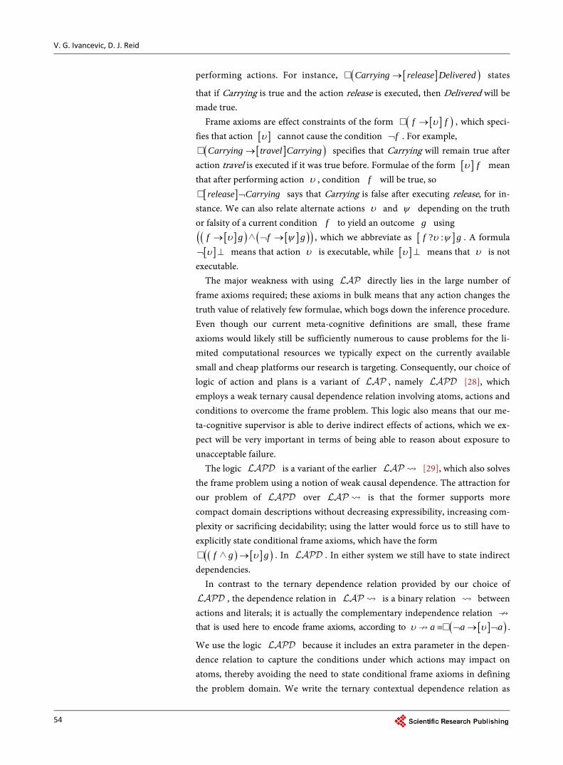
performing actions. For instance, [ ]( )Carrying release Delivered→ states

that if Carrying is true and the action release is executed, then Delivered will be made true.

Frame axioms are effect constraints of the form [ ]( )f fυ→ , which speci-fies that action [ ]υ cannot cause the condition f¬ . For example,

[ ]( )Carrying travel Carrying→ specifies that Carrying will remain true after action travel is executed if it was true before. Formulae of the form [ ] fυ mean that after performing action υ , condition f will be true, so [ ]release Carrying¬ says that Carrying is false after executing release, for in-

stance. We can also relate alternate actions υ and ψ depending on the truth or falsity of a current condition f to yield an outcome g using

[ ]( ) [ ]( )( )f g f gυ ψ→ ¬ →∧ , which we abbreviate as [ ]? :f gυ ψ . A formula [ ]υ¬ ⊥ means that action υ is executable, while [ ]υ ⊥ means that υ is not

executable. The major weakness with using directly lies in the large number of

frame axioms required; these axioms in bulk means that any action changes the truth value of relatively few formulae, which bogs down the inference procedure. Even though our current meta-cognitive definitions are small, these frame axioms would likely still be sufficiently numerous to cause problems for the li-mited computational resources we typically expect on the currently available small and cheap platforms our research is targeting. Consequently, our choice of logic of action and plans is a variant of , namely [28], which employs a weak ternary causal dependence relation involving atoms, actions and conditions to overcome the frame problem. This logic also means that our me-ta-cognitive supervisor is able to derive indirect effects of actions, which we ex-pect will be very important in terms of being able to reason about exposure to unacceptable failure.

The logic is a variant of the earlier [29], which also solves the frame problem using a notion of weak causal dependence. The attraction for our problem of over is that the former supports more compact domain descriptions without decreasing expressibility, increasing com-plexity or sacrificing decidability; using the latter would force us to still have to explicitly state conditional frame axioms, which have the form

( ) [ ]( )f g gυ→ ∧ . In . In either system we still have to state indirect dependencies.

In contrast to the ternary dependence relation provided by our choice of , the dependence relation in is a binary relation between actions and literals; it is actually the complementary independence relation that is used here to encode frame axioms, according to [ ]( )a a aυ υ≡ ¬ → ¬ .

We use the logic because it includes an extra parameter in the depen-dence relation to capture the conditions under which actions may impact on atoms, thereby avoiding the need to state conditional frame axioms in defining the problem domain. We write the ternary contextual dependence relation as

V. G. Ivancevic, D. J. Reid

55

f aυ , where f is a classical formula, Vυ ∈ is a verb and a A∈ is an atom, to mean that if f is true then action υ may change the truth value of a . Note that weak contextual dependence does not mean that the action in the context causes a change in truth value of the atom, only that the change might happen. For instance, Carrying Delivered release Delivered¬ ∧ states that executing release when Carrying is true and Delivered is false may effect the value of Delivered; the conditional frame axiom

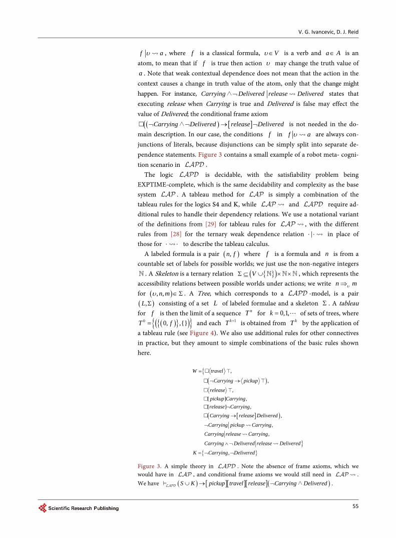
( ) [ ]( Carrying Delivered release Delivered¬ ¬ → ¬ ∧ is not needed in the do-main description. In our case, the conditions f in f aυ are always con-junctions of literals, because disjunctions can be simply split into separate de-pendence statements. Figure 3 contains a small example of a robot meta- cogni-tion scenario in .

The logic is decidable, with the satisfiability problem being EXPTIME-complete, which is the same decidability and complexity as the base system . A tableau method for is simply a combination of the tableau rules for the logics S4 and K, while and require ad-ditional rules to handle their dependency relations. We use a notational variant of the definitions from [29] for tableau rules for , with the different rules from [28] for the ternary weak dependence relation |⋅ ⋅ in place of those for ⋅ ⋅ to describe the tableau calculus.

A labeled formula is a pair ( ),n f where f is a formula and n is from a countable set of labels for possible worlds; we just use the non-negative integers . A Skeleton is a ternary relation { }( )VΣ ⊆ ∪ × × , which represents the accessibility relations between possible worlds under actions; we write n mυ⇒ for ( ), ,n mυ ∈Σ . A Tree, which corresponds to a -model, is a pair ( ),L Σ consisting of a set L of labeled formulae and a skeleton Σ . A tableau for f is then the limit of a sequence nT for 0,1,k = of sets of trees, where

( ){ }( ){ }0 0, ,{}T f= and each 1kT + is obtained from kT by the application of a tableau rule (see Figure 4). We also use additional rules for other connectives in practice, but they amount to simple combinations of the basic rules shown here.

{( )

[ ]( )

,

,

, [ ] , [ ] ,

,

,

W travel

Carrying pickup

releasepickup Carryingrelease Carrying

Carrying release Delivered

Carrying pickup Carrying

Carrying releas

=

¬ →

¬

→

¬

}{ }

,

,

e Carrying

Carrying Delivered release Delivered

K Carrying Delivered

∧¬

= ¬ ¬

Figure 3. A simple theory in . Note the absence of frame axioms, which we would have in , and conditional frame axioms we would still need in . We have ( ) [ ][ ][ ]( )S K pickup travel release Carrying Delivered∪ → ¬ ∧ .

V. G. Ivancevic, D. J. Reid

56

( ) ( ) ( ) ( )( ) ( ) ( )( ) ( ) ( ) ( )( ) ( )( ) ( )

( ){ }( )( ) ( ) ( )( ) ( )

1

: if , and , then add , to

: if , then add , to

: if , then add , and , to

: if , then add ,

and add , , to

: if , then add , to

4 : if , and

i

n f L n f L n L

n f L n f L

n f g L n f n g L

n f g L n f

L n g T

T n f L n f L

n f L n υ

+

⊥ ∈ ¬ ∈ ⊥

¬ ¬¬ ∈

∧ ∧ ∈

∨ ¬ ∧ ∈

∪ ¬ Σ

∈

∈ ⇒

( )( ) [ ]( ) ( )( ) [ ]( ) ( )

( ) ( ) ( )

for some or

then add , to

: if , and then add , to

: if , then add , to and to ,

where is new: if , ) then add , to and to ,

where is ne

V

m V n m

m f L

K n f L n m m f L

n f L m f L n m

mn f L m f L n m

m

υ

υ

υ

υ

υ

∈ ⇒

∈ ⇒

⟨⟩ ¬ ∈ ¬ ⇒ Σ

∈

◊ ¬ ∈ ¬ ⇒ Σ

∈

( ) ( ) ( )( )

( ) ( ) ( )( )

w: if , , where is a literal, , and , for all

then add , to

: if , , where is a literal, , and , for all

then add , to

RP n f L f n m L n g g f

m f L

RB m f L f n m L n g g f

n f L

υ

υ

υ

υ

∈ ⇒

∈ ⇒

Figure 4. Tableau rules for , as a modification of the tableau rules for , with the final two rules substituted for new rules for handling the ternary dependence re-lation. The notation ( ),L n a means that the literal a cannot be verified in world n

from the formulae in L .

The rule ( )RP states that all literals that depend on an action in a context that does not verify have to be propagated following the execution of that action. Rule ( )RB is a back-propagation rule, which is required for completeness of the tableau method, and it states that literals that are true but whose truth value was not changed from the parent node in the tree must also have been true in the parent node. See [29] and [28] for further details.

Space precludes a full account of our test implementation; our system is in the pure functional language Haskell. We use a straightforward algebraic type for representing formulas, and labeled formulas are represented using a simple type synonym. The ordering of the clauses is important: formulas causing tableau branching are lower in the definition, which means that the ordering on formu-las that the compiler generates by declaring the type to be an instance of “Ord” is used to prioritize reduction rule application to push branching towards the low-er part of the tableau.

data LAPFormula = F|T|Atom String|Not LAPFormula And Formula |Necessary LAPFormula|Possible LAPformula |Cause String Formula... deriving (Eq, Ord)

type Formula = (Int, Formula) Space precludes a complete account of our test implementation, so we offer an

abbreviated description focussing on the core components. In addition to the tableau evaluation module, we also have parser modules, and a number of sup-porting data structures particularly for representing skeleton relations and de-pendency relations. The tableau is implemented in operational semantics style,

V. G. Ivancevic, D. J. Reid

57

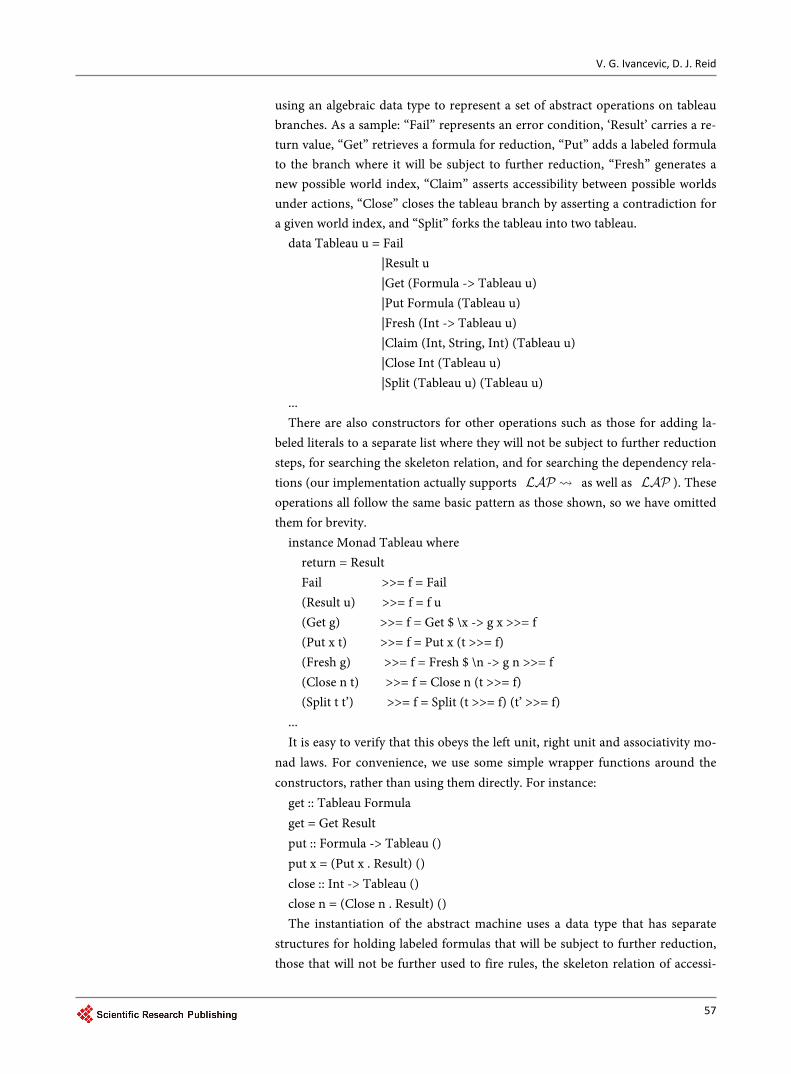
using an algebraic data type to represent a set of abstract operations on tableau branches. As a sample: “Fail” represents an error condition, ‘Result’ carries a re-turn value, “Get” retrieves a formula for reduction, “Put” adds a labeled formula to the branch where it will be subject to further reduction, “Fresh” generates a new possible world index, “Claim” asserts accessibility between possible worlds under actions, “Close” closes the tableau branch by asserting a contradiction for a given world index, and “Split” forks the tableau into two tableau.

data Tableau u = Fail |Result u |Get (Formula -> Tableau u) |Put Formula (Tableau u) |Fresh (Int -> Tableau u) |Claim (Int, String, Int) (Tableau u) |Close Int (Tableau u) |Split (Tableau u) (Tableau u)

... There are also constructors for other operations such as those for adding la-

beled literals to a separate list where they will not be subject to further reduction steps, for searching the skeleton relation, and for searching the dependency rela-tions (our implementation actually supports as well as ). These operations all follow the same basic pattern as those shown, so we have omitted them for brevity.

instance Monad Tableau where return = Result Fail >>= f = Fail (Result u) >>= f = f u (Get g) >>= f = Get $ \x -> g x >>= f (Put x t) >>= f = Put x (t >>= f) (Fresh g) >>= f = Fresh $ \n -> g n >>= f (Close n t) >>= f = Close n (t >>= f) (Split t t’) >>= f = Split (t >>= f) (t’ >>= f)

... It is easy to verify that this obeys the left unit, right unit and associativity mo-

nad laws. For convenience, we use some simple wrapper functions around the constructors, rather than using them directly. For instance:

get :: Tableau Formula get = Get Result put :: Formula -> Tableau () put x = (Put x . Result) () close :: Int -> Tableau () close n = (Close n . Result) () The instantiation of the abstract machine uses a data type that has separate

structures for holding labeled formulas that will be subject to further reduction, those that will not be further used to fire rules, the skeleton relation of accessi-

V. G. Ivancevic, D. J. Reid

58

bility between possible worlds, and the ternary dependency relation. Here “BBTree” is an ordered tree type that implements the priority relation on for-mulas, so that non-branching formulas are preferred for reduction over those that cause branching. “Skeleton” is an indexed tree structure supporting the various kinds of searches needed on accessibility relation instances, and “De-pendency” represents the ternary dependency relation and similarly allows the necessary searches on its instances.

data Branch = Branch { todo :: BBTree Formula , lits :: BBTree Formula , rho :: Skeleton , index :: Int , deps :: Dependency } deriving (Eq, Ord)

The central function is the “runTab” function that defines the how the ab-stract operations should be applied to branch structures. The rest of the cases (not shown) follow the same basic pattern.

runTab:: (Ord u) => Tableau u -> Branch -> BBTree (u, Branch) runTab Fail _ = nil runTab (Result y) b = singleton (y, b) runTab (Get g) b = case delmin (todo b) of

Nothing -> nil (Just x, xs) -> run (g x) (b { todo = xs})

runTab (Put f t) b = let b’ = into b f in runTab t b’

runTab (Fresh g) b = let n = 1 + ()index b) b’ = b {index = n} in runTab (g n) b’

runTab (Close n t) b = let b’ = b { todo = nil, lits = single (n, F) } in runTab t b’

runTab (Split t t’) b = (runTab t b) ‘mplus’ (runTab t’ b) ... The functions “nil” and “singleton” build trees with zero and one element,

respectively. The case for ‘Put’ uses an auxiliary function ‘into’ that checks first to see if the branch already contains the negation of the formula to be inserted into the branch and, if so, inserts a formula containing contradiction “F” instead. This approach provides us with a very compact and natural definition for the tableau reduction rules, as illustrated below.

reduce :: Formula -> Tableau () reduce (n, F) = close n reduce (n, T) = return () reduce (n, And x y) = put (n,x) >> put(n,y) reduce (n, Or x y) = put (n, x) ‘mplus’ put (n,y) reduce (n, Not (Necessary x)) = fresh >>= \n -> put (n’, neg x)

V. G. Ivancevic, D. J. Reid

59

>> claim (n, “[]”, n’) reduce (n, Necessary x) = put (n, x) >> fromN w

>>= mapM_ (\(_, m) -> put (m, Necessary x))) ... The second to last case implements rule ( )◊ The last case in the snippet im-

plements rules ( )T and ( )4 . It uses a function “fromN” that returns a list of verbs and world indexes accessible from a given world index, and the standard library “mapM” to map each of these to actions that insert each resulting formu-la into the branch. A program for the abstract tableau machine for completely expanding a branch is also very simple.

expand :: Tableau () expand = isComplete >>= \c -> if c then return ()

else get >>= reduce >> reduction Given an initial branch, the tableau can be applied to an initial branch, say b,

with runTab expand b. We also have a number of convenience functions for producing an initial branch data structure from a list of formulas and depen-dency relation instances, and for extracting the results from the resulting tree of closed and saturated branches. Their implementation is straightforward though somewhat tedious.

6. Conclusions

In this paper, we have presented sophisticated cognitive and meta-cognitive su-pervisor models for joint swarms of robotic aerial and ground vehicles. Based on the research of the recent Nobel prize in Physiology on path integration and na-vigation in the mammalian and human hippocampus (briefly reviewed in the appendix), this paper develops a Hamiltonian path integral cognitive supervisor model. This model emulates an ∞ -dimensional neural recurrent neural net-work, yielding attractor fields for robotic swarms. While direct simulation of this Hamiltonian path integral can be done using IBMs’s TrueNorth chip, for the purpose of its immediate evaluation on common hardware, we have transformed this into a coupled pair of NLS equations and simulated this in Mathematica.

The central point of our meta-cognitive model is that we are not utilising in-ference in modal logic systems to determine low-level movement, but rather to simulate a kind of high-level awareness in light of descriptive goals, general con-ditions and broad actions to make sense of sensor data and guide overall vehicle behaviour. Our representation of meta-cognitive communication using simple atoms and verbs reflects this choice. By effectively delegating details, the rela-tively simple models are supported by the propositional multi-modal logic suffice, with decidability of inference and, in practice, reasonable computation costs and fairly compact meta-cognitive behavioural definitions. We plan to supplant our current use of a tableau method for meta-cognitive in-ference using the multimodal logic with a new path integral represen-tation; that is, to eventually fully integrate meta-cognition and affine Hamilto-nian control into what would amount to a single coherent generalized Hopfield

V. G. Ivancevic, D. J. Reid

60

type recurrent neural network.

Acknowledgements

The authors are grateful to Dr Yi Yue and Dr Martin Oxenham, Decision Sciences, Joint and Operations Analysis Division, DST Group, Australia—for their constructive comments which have improved the quality of this paper. This work is a part of the DSTG TAS SRI (Tyche) project.

References [1] Ivancevic, V. and Yue, Y. (2016) Hamiltonian Dynamics and Control of a Joint Au-

tonomous Land-Air Operation. Nonlinear Dynamics, 84, 1853-1865. https://doi.org/10.1007/s11071-016-2610-y

[2] McNaughton, B.L., Battaglia, F.P., Jensen, O., Moser, E.I. and Moser, M.-B. (2006) Path Integration and the Neural Basis of the Cognitive Map. Nature Reviews Neu-roscience, 7, 663-678. https://doi.org/10.1038/nrn1932

[3] Moser, E.I., Kropff, E. and Moser, M.-B. (2008) Place Cells, Grid Cells, and the Brain’s Spatial Representation System. Annual Review of Neuroscience, 31, 69-89. https://doi.org/10.1146/annurev.neuro.31.061307.090723

[4] O’Keefe, J., Burgess, N., Donnett, J.G., Jeffery, K.J. and Maguire, E.A. (1998) Place Cells, Navigational Accuracy, and the Human Hippocampus. Philosophical Trans-actions of the Royal Society of London A, 353, 1333-1340. https://doi.org/10.1098/rstb.1998.0287

[5] Monteiro, S., Vaz, M. and Bicho, E. (2004) Attractor Dynamics Generates Robot Formation, from Theory to Implementation. International Conference on Robotics and Automation, Vol. 3, New Orleans, 26 April-1 May 2004, 2582-2586. https://doi.org/10.1109/robot.2004.1307450

[6] O’Keefe, J. (1976) Place Units in the Hippocampus of the Freely Moving Rat. Expe-rimental Neurology, 51, 78-109. https://doi.org/10.1016/0014-4886(76)90055-8

[7] O’Keefe, J. and Nadel, L. (1978) The Hippocampus as a Cognitive Map. Clarendon Press, Oxford.

[8] Ivancevic, V. and Ivancevic, T. (2008) Complex Nonlinearity, Chaos, Phase Transi-tions, Topology Change and Path Integrals. Springer, New York.

[9] Ivancevic, V. and Reid, D. (2015) Complexity and Control, towards a Rigorous Be-havioral Theory of Complex Dynamical Systems. World Scientific, Singapore.

[10] Feynman, R.P. (1951) An Operator Calculus Having Applications in Quantum Electrodynamics. Physical Review, 84, 108-128. https://doi.org/10.1103/PhysRev.84.108

[11] Feynman, R.P. (1948) Space-Time Approach to Non-Relativistic Quantum Me-chanics. Reviews of Modern Physics, 20, 267. https://doi.org/10.1103/RevModPhys.20.367

[12] Ivancevic, V., Reid, D. and Scholz, J. (2014) Action-Amplitude Approach to Con-trolled Entropic Self-Organization. Entropy, 16, 2699-2712. https://doi.org/10.3390/e16052699

[13] Hopfield, J.J. (1982) Neural Networks and Physical Systems with Emergent Collec-tive Computational Abilities. Proceedings of the National Academy of Sciences, 79, 2554-2558. https://doi.org/10.1073/pnas.79.8.2554

[14] Hopfield, J.J. (1984) Neurons with Graded Response Have Collective Computation-

V. G. Ivancevic, D. J. Reid

61

al Properties Like Those of Two-State Neurons. Proceedings of the National Acad-emy of Sciences, 81, 3088-3092. https://doi.org/10.1073/pnas.81.10.3088

[15] Service, R.F. (2014) The Brain Chip. Science, 345, 614-668. https://doi.org/10.1126/science.345.6197.614

[16] Ivancevic, V. and Ivancevic, T. (2009) Quantum Neural Computation. Springer, Berlin.

[17] Ivancevic, V. and Reid, D. (2012) Turbulence and Shock-Waves in Crowd Dynam-ics. Nonlinear Dynamics, 68, 285-304. https://doi.org/10.1007/s11071-011-0227-8

[18] Ivancevic, V. (2010) Adaptive-Wave Alternative for the Black-Scholes Option Pric-ing Model. Cognitive Computation, 2, 17-30. https://doi.org/10.1007/s12559-009-9031-x

[19] Ivancevic, V. (2011) Adaptive Wave Models for Sophisticated Option Pricing. Journal of Mathematical Finance, 1, 41-49. https://doi.org/10.4236/jmf.2011.13006

[20] Manakov, S.V. (1974) On the Theory of Two-Dimensional Stationary Self-Focusing of Electromagnetic Waves. Soviet Physics, 38, 248-253. (In Russian)

[21] Lax, P. (1968) Integrals of Nonlinear Equations of Evolution and Solitary Waves. Communications on Pure and Applied Mathematics, 21, 467-490. https://doi.org/10.1002/cpa.3160210503

[22] Haelterman, M. and Sheppard, A.P. (1994) Bifurcation Phenomena and Multiple Soliton Bound States in Isotropic Kerr Media. Physical Review E, 49, 3376-3381. https://doi.org/10.1103/PhysRevE.49.3376

[23] Yang, J. (1997) Classification of the Solitary Wave in Coupled Nonlinear Schrödin-ger Equations. Physica D, 108, 92-112. https://doi.org/10.1016/S0167-2789(97)82007-6

[24] Hanm, S.-H. and Koh, I.G. (1999) Stability of Neural Networks and Solitons of Field Theory. Physical Review E, 60, 7608-7611. https://doi.org/10.1103/PhysRevE.60.7608

[25] Fisher, M.J. and Ladner, R.E. (1979) Propositional Dynamic Logic of Regular Pro-grams. Journal of Computer and System Sciences, 18, 194-211. https://doi.org/10.1016/0022-0000(79)90046-1

[26] Zhang, D. and Foo, N.Y. (2001) EPDL, a Logic for Causal Reasoning. Proceedings of the IJCAI 2001, Seattle, 4-10 August 2001, 131-138.

[27] Hughes, G.E. and Cresswell, M.J. (1996) A New Introduction to Modal Logic. Rout-ledge, Abingdon-on-Thames. https://doi.org/10.4324/9780203290644

[28] Castilho, M.A., Herzig, A. and Varzinczak, I. (2002) It Depends on the Context! A Decidable Logic of Actions and Plans Based on a Ternary Dependence Relation. NMR’02, Toulouse, 19-21 April 2002, 343-348.

[29] Castilho, M.A., Gasquet, O. and Herzig, A. (1999) Formalizing Action and Change in Modal Logic 1, the Frame Problem. Journal of Logic and Computation, 9, 701- 735. https://doi.org/10.1093/logcom/9.5.701

[30] Hebb, D.O. (1949) The Organization of Behavior. Wiley, New York.

[31] O’Keefe, J. and Dostrovsky, J. (1971) The Hippocampus as a Spatial Map, Prelimi-nary Evidence from Unit Activity in the Freely Moving Rat. Brain Research, 34, 171-175. https://doi.org/10.1016/0006-8993(71)90358-1

[32] Mittelstaedt, M.L. and Mittelstaedt, H. (1980) Homing by Path Integration in a Mammal. Naturwissenschaften, 67, 566-567. (In German) https://doi.org/10.1007/BF00450672

[33] Ranck, J.B. (1985) Electrical Activity of the Archicortex. Akademiai Kiado, Budap-

V. G. Ivancevic, D. J. Reid

62

est, 217-220.

[34] Bostock, E., Muller, R.U. and Kubie, J.L. (1991) Experience-Dependent Modifica-tions of Hippocampal Place Cell Firing. Hippocampus, 1, 193-205. https://doi.org/10.1002/hipo.450010207

[35] McNaughton, B.L., Chen, L.L. and Markus, E.J. (1991) “Dead Reckoning”, Land-mark Learning, and the Sense of Direction, a Neurophysiological and Computa-tional Hypothesis. Journal of Cognitive Neuroscience, 3, 190-202. https://doi.org/10.1162/jocn.1991.3.2.190

[36] Wilson, M.A. and McNaughton, B.L. (1993) Dynamics of the Hippocampal Ensem-ble Code for Space. Science, 261, 1055-1058. https://doi.org/10.1126/science.8351520

[37] O’Keefe, J. and Recce, M.L. (1993) Phase Relationship between Hippocampal Place Units and the EEG Theta Rhythm. Hippocampus, 3, 317-330. https://doi.org/10.1002/hipo.450030307

[38] McNaughton, B.L., et al. (1996) Deciphering the Hippocampal Polyglot, the Hippo-campus as a Path Integration System. Journal of Experimental Biology, 199, 173- 185.

[39] Tsodyks, M. and Sejnowski, T. (1995) Associative Memory and Hippocampal Place Cells. International Journal of Neural Systems, 6, S81-S86.

[40] Zhang, K. (1996) Representation of Spatial Orientation by the Intrinsic Dynamics of the Head-Direction Cell Ensemble, a Theory. Journal of Neuroscience, 16, 2112- 2126.

[41] Samsonovich, A. and McNaughton, B.L. (1997) Path Integration and Cognitive Mapping in a Continuous Attractor Neural Network Model. Journal of Neuros-cience, 17, 5900-5920.

[42] O’Keefe, J. (1999) Do Hippocampal Pyramidal Cells Signal Non-Spatial as Well as Spatial Information? Hippocampus, 9, 352-364. https://doi.org/10.1002/(SICI)1098-1063(1999)9:4<352::AID-HIPO3>3.0.CO;2-1

[43] Fyhn, M., Molden, S., Witter, M.P., Moser, E.I. and Moser, M.-B. (2004) Spatial Re-presentation in the Entorhinal Cortex. Science, 305, 1258-1264. https://doi.org/10.1126/science.1099901

[44] Hafting, T., Fyhn, M., Molden, S., Moser, M.-B. and Moser, E.I. (2005) Microstruc-ture of a Spatial Map in the Entorhinal Cortex. Nature, 436, 801-806. https://doi.org/10.1038/nature03721

[45] Witter, M.P. and Moser, E.I. (2006) Spatial Representation and the Architecture of the Entorhinal Cortex. Trends in Neurosciences, 29, 671-678. https://doi.org/10.1016/j.tins.2006.10.003

[46] O’Keefe, J. and Burgess, N. (2005) Dual Phase and Rate Coding in Hippocampal Place Cells, Theoretical Significance and Relationship to Entorhinal Grid Cells. Hippocampus, 15, 853-866. https://doi.org/10.1002/hipo.20115

[47] Solstad, T., Moser, E.I. and Einevoll, G.T. (2006) From Grid Cells to Place Cells, a Mathematical Model. Hippocampus, 16, 1026-1031. https://doi.org/10.1002/hipo.20244

[48] Burgess, N., Barry, C. and O’Keefe, J. (2007) An Oscillatory Interference Model of Grid Cell Firing. Hippocampus, 17, 801-812. https://doi.org/10.1002/hipo.20327

[49] Yartsev, M.M. and Ulanovsky, N. (2013) Representation of Three-Dimensional Space in the Hippocampus of Flying Bats. Science, 340, 367-372. https://doi.org/10.1126/science.1235338

V. G. Ivancevic, D. J. Reid

63

[50] Yartsev, M.M. (2013) Space Bats, Multidimensional Spatial Representation in the Bat. Science, 342, 573-574. https://doi.org/10.1126/science.1245809

[51] Turing A.M. (1990) The Chemical Basis of Morphogenesis. Philosophical Transac-tions of the Royal Society B, 237, 37-72. https://doi.org/10.1007/BF02459572

V. G. Ivancevic, D. J. Reid

64

Appendix

Hippocampal Path Integration and Navigation in Mammals and Humans We start with a brief history of hippocampal navigation, from O’Keefe’s pio-

neering work to the discovery of grid cells by Mosers. While most of neural network theory (including the concepts of associative

synaptic plasticity, cell assemblies and phase sequences) is founded on Hebb’s seminal work [30], and hippocampus as a spatial cognitive map was proposed in [7] [31], the pioneering paper on hippocampal navigation was [6], in which O’Keefe proposed a theoretical suggestion of a landmark-independent naviga-tional system upstream of the hippocampus. A few years later, path integration in mammals was reported in [32], followed by a quantitative description of head direction-sensitive cells in the brain by [33], a report of remapping in hippo- campal place cells in [34], and an early version of the head-direction path-inte- grator model in [35], which formed the conceptual basis of subsequent conti-nuous attractor models for path integration.

A landmark paper [36] introduced empirical understanding of hippocampal neurodynamics, by the ability to record simultaneously from many neurons in the freely behaving animal. The phase relationship between hippocampal place units and the EEG theta rhythm was shown in [37], and the hippocampus as a path-integration system was proposed in [38].

A series of continuous attractor papers started with [39], followed by an at-tractor model of head direction cell by angular velocity integration in [40] and the introduction of the concept of periodic boundaries and an early introduction of medial entorhinal grid cells in mammals by [41].

Next two papers by O’Keefe, [4] [42], consider human hippocampus place cells, which are signaling both spatial and non-spatial information.

The pioneering study [43] reports that spatial position is represented accu-rately among ensembles of principal neurons in superficial layers of the medial entorhinal cortex (MEC), while the scale of representation increases along the MEC’s dorsoventral axis. It is followed by [44] that reports the discovery of grid cells, which are suggested as a foundation for a universal path integration-based neuronal map of the spatial environment. Spatial representation and the archi-tecture of the entorhinal cortex was presented in [45].

Next, we give a current brief overview of hippocampal formation: place cells and grid cells.

The review paper [2] shows that the hippocampal formation is able to encode relative spatial location of mammals and humans (without any reference to ex-ternal cues) by the integration of translational and rotational self-motion, which is called the path integration.

Both theoretical and empirical studies show that the synaptic matrix of the MEC-grid cells of young mammals perform heavy self-organizing path-integra- tion computations, similar to Turing’s symmetry-breaking operation5, while the

5A landmark Turing’s paper [51] demonstrating that symmetry breaking can occur in the simple reaction-diffusion system, that results in spatially periodic structures can account for pattern forma-tion in nature.

V. G. Ivancevic, D. J. Reid

65

scale at which space is represented increases systematically along the dorsoven-tral axis in both the hippocampus and the MEC. Spatially periodic inputs (at multiple scales) converging from the MEC-grid cells, result in non-periodic spa-tial firing of the hippocampal place cells.

The paper [3] reviews how place cells and grid cells form the entorhinal-hip- pocampal representations, initially observed in [46] and mathematically mod-eled in [47] [48], for quantitative spatio-temporal representation of places, routes, and associated experiences during behavior and in memory.

It has been observed that place cells perform both pattern completion and pattern separation, while hippocampal representations cannot always be discon- tinuous as in a sequential Hopfield network [13], but rather similar to the graded-response Hopfield network [14].

Finally, while all the research mentioned so far was dealing with 2D hippo-campal path integration and navigation, which is relevant for our UGVs, in re-cent years this research has been generalized to 3D navigation of bats in [49] [50].

Submit or recommend next manuscript to SCIRP and we will provide best service for you:

Accepting pre-submission inquiries through Email, Facebook, LinkedIn, Twitter, etc. A wide selection of journals (inclusive of 9 subjects, more than 200 journals) Providing 24-hour high-quality service User-friendly online submission system Fair and swift peer-review system Efficient typesetting and proofreading procedure Display of the result of downloads and visits, as well as the number of cited articles Maximum dissemination of your research work

Submit your manuscript at: http://papersubmission.scirp.org/ Or contact ica@scirp.org