ORIGINAL PAPER

Coarse-grained model of the native cellulose Ia and thetransformation pathways to the Ib allomorph

Adolfo B. Poma . Mateusz Chwastyk .

Marek Cieplak

Received: 31 December 2015 / Accepted: 3 March 2016 / Published online: 16 March 2016

� Springer Science+Business Media Dordrecht 2016

Abstract All-atom simulations are used to derive

effective parameters for a coarse-grained description

of the crystalline cellulose Ia. In this description,

glucose monomers are represented by the C4 atoms

and non-bonded interactions within the cellulose

sheets and between the sheets by effective Lennard-

Jones interactions. The parameters are determined by

two methods: the Boltzmann inversion and through

monitoring of the energies associated with changes of

the coarse-grained degrees of freedom. We find that

the stiffness-related parameters for cellulose Ia are

nearly the same as for Ib allomorph. However, the

non-bonded terms are placed differently and are

weaker leading to an overall lower energy, and free

energy, of Ib compared to Ia. We apply the coarse-

grained description to determine amorphous transition

states for the room-temperature conversion process

between the Ia and Ib allomorphs and to characterize

the interface between the crystalline forms of the

allomorphs.

Keywords Force field � Coarse-grained simulation �Cellulose Ia and Ib � Full-length microfibril �Conversion process � Free energy

Introduction

Cellulose is one of the most abundant renewable

biopolymers. It has been a subject of interest for a

broad scientific community. Examples of the recent

research are in the context of bioconversion of

cellulosic wastes into fermentable sugars to make

biofules (Bayer et al. 2007, 2010; Dashtban 2009;

Peplow 2014) and in the design of high-performance

materials that involve nanocellulose fibers (Lee et al.

2014; Hakansson et al. 2014).

Cellulose consists of unbranched homopolysaccha-

ride chains of glucopyranose units, denoted as D-GLC.

Two D-GLC units are linked via bð1 ! 4Þ-glycosidic

bonds which connect the C1 and C4 carbon atoms. The

chains can combine into various allomorphic struc-

tures that may coexist. Two of them, Ia and Ib are

crystalline and their relative abundance ratio depends

on the source of cellulose (Newman 1999; Kataoka

and Kondo 1999). Cellulose Ia is the main constituent

of the cell walls of the green algae Cladophora

(Mihranyan et al. 2007) and Valonia (Revol 1982),

whereas the celluloses from the higher plants, such as

cotton, wood and ramie are rich in the Ib allomorph. At

one extreme, the cellulose produced by a marine

animal, tunicate, is nearly 100 % Ib (Nishiyama et al.

2002). At another, the cellulose of the cell wall of the

alga Glaucocystis can be considered as almost 100 %

Ia (Imai et al. 1999).

The crystal structures of cellulose Ia and Iballomorphs have been characterized by means of

A. B. Poma (&) � M. Chwastyk � M. Cieplak

Institute of Physics, Polish Academy of Sciences, Aleja

Lotnikow 32/46, 02-668 Warsaw, Poland

e-mail: poma@ifpan.edu.pl

123

Cellulose (2016) 23:1573–1591

DOI 10.1007/s10570-016-0903-4

synchrotron X-ray and neutron diffraction (Nishiyama

et al. 2003, 2008). In both allophorms, cellulose

chains are parallel and aligned along the same growth

direction (coinciding with the crystallographic c-axis)

as shown in Fig. 1. It has been found that cellulose Iaand cellulose Ib differ in mutual packing of the chains.

The Ia allomorph has a triclinic unit cell of P1

symmetry with a single cellobiose unit as basis with

layers displaced along the c-axis by ?c/4. Ib has a

monoclinic unit cell of the P21 symmetry with two

cellobiose units forming a basis—they are termed

origin (OR) and center (CE). Ib is thus made of two

different sheets which are displaced by ?c/4 and �c/4

in an alternating fashion. The differences between the

two crystalline allomorphs are captured by the inter-

chain radial distribution function (denoted as RDF)

shown in Fig. 2. Details of the RDF calculation will be

presented in section IIIB. The RDF used here

describes the probability of finding a C4 atom in an

infinitesimal volume element at distance r from

another C4 atom on a different chain. The RDF

patterns are seen to deviate in the locations and heights

of the corresponding peaks. The shift in the locations

is slight for the first and fourth peaks, but is more

visible in the case of the second and third peaks. The

first peak for Ib is about 40 % taller than for Ia and is

located near r of 6 A. The difference in the height of

the first peak in the RDF between the two allomorphs

is attributed to a non-uniform distance distribution of

the four closest neighbours (see Fig. 2b). In the case of

Ib, these neighbours remain at similar equilibrium

distances (see Fig. 2c), whereas in Ia they fluctuate

within a much larger range (see Fig. 2d).

The two different crystalline structures necessarily

come with distinct placements of the hydrogen bonds

(HB). There is a relatively strong presence of the

O3–H� � �O5 intrachain and O6–H� � �O3 interchain

HBs which are responsible for the stability of the

layered structures. Experiments (Nishiyama et al.

2003) indicate the absence of the O–H� � �O interactions

between layers, but they suggest a larger presence of

the C–H� � �O intersheet HBs in the Ib allophorm

compared to the Ia one. Thus, it is expected that some

C–H� � �O hydrogen bonds and van der Waals forces

contribute to the larger stability of Ib over Ia.

Different coarse grained models of cellulose have

been developed to address important questions con-

nected to the processing of plant biomass. Among

them we can distinguish those related to (1)

characterization of crystalline and amorphous cellu-

lose phases (Molinero and Goddard 2004; Wohlert and

Berglund 2011; Fan and Maranas 2014; Srinivas et al.

2014; Queyroy et al. 2004; Lopez et al. 2015), (2) the

transition from cellulose Ib to cellulose IIII (Bellesia

et al. 2012), and (3) understanding of the protein–

polysaccharide interaction (Poma et al. 2015; Bu et al.

2010). However, none of these models describes the Iaallomorph nor it considers the interconversion process

into Ib allomorph.

Here, we extend our previous coarse-grained (CG)

description of Ib (Poma et al. 2015) to the Iaallomorph to bring out differences in the effective

dynamical parameters between the two structures. The

bonded interactions within the chains are found to be

about the same, but the strengths of the effective non-

bonded couplings differ. We employ the Boltzmann

Inversion (BI) approach (Meyer et al. 2000; Jochum

et al. 2012) and our own energy-based (EB) method

(Poma et al. 2015). Our previous study (Poma et al.

2015) has been focused on cellulose Ib and two

hexaoses. While the BI and EB methods agree in their

account of the bonded parameters they disagree when

dealing with non-bonded terms. However, the EB

approach is deemed to be more reliable as it yields

parameters which agree with experimental data on the

strength of HBs in solids (Steiner 2002). We test our

CG model and its parameters by making comparisons

to all-atom simulations. In particular, we consider the

RDFs and demonstrate the agreement between the two

descriptions for both allomorphs.

We then turn our attention to the phase transfor-

mations between the Ia and Ib structures. Conversion

of Ia into Ib is usually accomplished through

hydrothermal heating at the temperature (T) between

533 and 553 K. The process lasts for more than half an

hour (Wada et al. 2003). On heating, cellulose Ia gets

cFig. 1 a shows the 36-chain microfibril model of the cellulose

Ia allomorph as viewed in the plane perpendicular to the c axis

(i.e. the polymerization axis). Axes a and b define the triclinic

unit cell formed by one chain. b Shows the layer packing in

cellulose Ia. The layers are displaced along the c-axis by þc=4.

Monomers shown in blue indicate the first D-GLC monomers in

each layer. c, d are similar to a, d respectively but they illustrate

the structure of Ib. In this case, the unit cell is monoclinic. It is

formed by two chains named origin (OR) and center (CE). A

minimum number of chains for each allomorph is represented

inside the unit cell (dashed black line). Layers in the Iballomorph alternate between þc=4 and �c=4 displacements.

(Color figure online)

1574 Cellulose (2016) 23:1573–1591

123

Cellulose (2016) 23:1573–1591 1575

123

converted to an amorphous high temperature phase

that turns into the Ib allomorph upon subsequent

cooling. This kind of experiment is the main reason

behind the common belief that the Ib phase has a lower

free energy than the Ia one (Debzi et al. 1991;

Matthews et al. 2011). The conversion to Ib has great

implications for industrial processes such as the dilute

acid pretreatment of poplar and switchgrass. It has

been observed (Foston and Ragauskas 2010) that the

relative amount of the cellulose Ia form decreases

while the relative amount of Ib allomorph increases

with the duration of the process. A similar result has

been reported for pretreatment of loblolly pines

(Sannigrahi et al. 2008). The Ia allomorph is used

industrially more often than Ib because of its higher

reactivity towards acetylation (Sassi et al. 2000). In

particular, it has been used for the production of

cellulose derivatives such as bioplastic (Nawrath et al.

1995), artificial textile fibers (Eadie and Ghosh 2011),

medical products (Lin and Dufresne 2014), etc.

However, extraction of cellulose Ia from its sources

(wood, corn stalk, cotton, etc) carries serious envi-

ronmental costs and new methods to provide it are

needed. One of the model organisms considered in the

context of the environmentally friendly I�a biosyn-

thesis is Acetobacter xylinum (Lee et al. 2013). It

should also be noted that the transformations between

I�b and I�a are expected to be facilitated by bending

the microfiber during its formation (Jarvis 2000).

Currently, no industrial process seems to have incor-

porated bending into the production of low cost

cellulose Ia.

The timescale involved in the conversion process is

beyond the capabilities of current all-atom simulations

aimed at testing this expectation. New computational

methods involving collective variables (Yu et al.

d4d3

d2

d1

r( A)

RDF

12.08.04.0

10

5

0

IαIβ

(a) (b)

r( A)

freq

uenc

y

7.06.05.0

4.0

2.0

0.0

d1(c)

r( A)

freq

uenc

y

7.06.05.0

4.0

2.0

0.0

d1(d)

Fig. 2 a shows RDF for the C4 atoms in the crystalline

cellulose Ia (solid line) and Ib (dashed line). The positions of the

first four peaks along the r-axis are indicated by the vertical

arrows next to the symbol ‘‘di’’ where the subscript i ranges

between 1 and 4. It counts the peaks in the ascending order. The

green arrows correspond to Ib and those in the black color to Ia.

b shows four cellulose chains surrounding one central chain in

the C4 representation. The eight C4 atoms which are closest to

an arbitrary C4 atom (in blue) from the central chain are

connected by sticks. The four blue sticks connect to atoms which

contribute to first peak in RFD—located at d1. The four red

sticks connect to atoms contributing to the second peak at d2. c,

d Show the the distributions in the values of d1 for the four

closest neighbors in Ib and Ia respectively. The thicker lines

corresponds to the neighbor for which the distribution is closest

to the first peak position in the RDF. The results were obtained

through all-atom simulations at room temperature. (Color

figure online)

1576 Cellulose (2016) 23:1573–1591

123

2014; Martonak et al. 2005) may enable such model-

ing in the future. In the past, all-atom simulation

studies were carried out to induce the conversion only

in one unit cell (with periodic boundary conditions)

(Hardy and Sarko 1996; Kroon-Batenburg et al. 1996)

whereas our CG model can capture larger-scale

structural reorganization inside the fibril. We thus

use our CG model to study the conversion process not

through a temperature cycling but through switching

of the CG non-bonded terms between the two phases.

We provide the energy characterization and confirm

that the Ib phase is indeed more stable. We also

determine the pathway of the conversion and the

transition state. The conformation corresponding to

the transition state can be a good starting point to study

properties of the amorphous cellulose. Obtaining an

amorphous state through heating turns out to be

impractical computationally.

Methods

We have considered fibers made of 36 chains, 80

D-GLC monomers each. The chains are packaged into

a nearly hexagonal shape as in ref. (Ding and Himmel

2006; Srinivas et al. 2014). When determining the CG

parameters, we focus on a central 7-chain subset of

this system.

All-atom molecular dynamics simulations

The molecular dynamics (MD) simulations were

conducted with version 2.9 of the NAMD package

(Phillips et al. 2005). The crystalline fibril of cellulose

Ia was parametrized by GLYCAM-06 force field

(Kirschner et al. 2008; Tessier et al. 2008). A solva-

tion box was used with 120 000 TIP3P water

molecules Jorgensen et al. (1983) to allow for struc-

tural relaxation of the ideal crystalline structure

prepared with the cellulose-builder toolkit (Gomes

and Skaf 2012). Periodic boundary conditions were

used and the electrostatic terms were counted by

employing the Particle Mesh Ewald method (Darden

et al. 1993) with a grid spacing of 1 A in all directions.

Numerical integration of Newton’s equations of

motion involved the time step of 1 fs and the atomic

coordinates were saved every 1 ps for analysis. The

system equilibration was carried out by first minimiz-

ing the energy in 1000 steps and then by implementing

a short 0.5 ns run in the NPT ensemble to achieve the

atmospheric pressure of 1 bar. The production runs

were carried out in the NVT ensemble at 300 K and

they lasted for 20 ns. The temperature was controlled

by the standard Langevin algorithm and the pressure

by the Langevin piston pressure control algorithm.

The MDenergy plugin from the VMD package

(Humphrey et al. 1996) was used to compute the

contributions of bonded and non-bonded energies.

Coarse-grained simulations

In our previous work on Ib and hexaoses (Poma et al.

2015), we have discussed two choices of representing

the sugar units by effective atoms: either the effective

atoms are placed at the center of mass of the D-GLC

unit or at the location of the C4 atom. We have found

the latter representation to be more stable numerically.

This approach is conceptually more akin to represent-

ing amino acids by the a-C atoms in many CG models

of proteins. Furthermore, the C4-based description

was shown (Poma et al. 2015) to be able to distinguish

between cellohexaose and mannohexaose which are

stereoisomers whereas the other representation could

not. Therefore, we use the C4 representation in our CG

model for cellulose Ia, as illustrated in Fig. 3. Our CG

simulations follow the scheme used for proteins

(Sułkowska and Cieplak 2007; Sikora et al. 2009)

and were carried out with an implicit solvent at 300 K

which corresponds to kBT ¼ 0:59 kcal/mol (kB is the

Boltzmann constant). The Langevin equations of

motion are used for thermostating and mimicking the

presence of the solvent. They are solved by a fifth

order predictor–corrector scheme. We simulate each

cellulose fibril for 5000s steps, where s is of order

1 ns.

Bonded interactions and their effective strengths

will be derived in the next sections. The strength of the

effective non-bonded interaction, �eff , depends on the

type of the HB. Our method involves reading of the

positions of the C4 atoms from an initial microfibril

cellulose structure and then using this information to

derive the length parameters reffij for the Lennard-

Jones (12–6) potential between the effective atoms.

Cellulose (2016) 23:1573–1591 1577

123

Boltzmann inversion method

The BI method (Meyer et al. 2000; Jochum et al.

2012) allows for determination of parameters in a CG

model by focusing on some degrees of freedom, q’s,

such as the distance between the effective atoms or the

bond angles formed by three sequentially consecutive

effective atoms. The assumption is that, in the

canonical ensemble corresponding to temperature T,

independent degrees of freedom obey the Boltzmann

distribution PðqÞ ¼ Z�1e�UðqÞ=kBT . Here, Z ¼Re�UðqÞ=kBTdq is the partition function. P(q) can be

determined through the atomistic simulation of the

reference system. Once this is done, one can derive the

corresponding effective potential U(q), also known as

the potential of the mean force, through the inversion

UðqÞ ¼ �kBT lnPðqÞ. Note that Z enters U(q) only as

an additive constant.

Energy-based approach for calculation of effective

bonded interactions

An alternative method (Poma et al. 2015) used here is

to fit the mean atomistic energies to the functional

dependence on q as postulated in the CG model. This

approach does not assume that the variables q are truly

independent. The first example is the effective bond

potential, Vabb which is defined between two effec-

tive atoms a and b in a biopolymer. The atoms

are separated by a time-dependent distance ra;b ¼jRa � Rbj which, generically, will be denoted as r. We

assume that

Vabb ðRa;Rbjkr; r0Þ ¼

1

2kr rab � r

ab0

� �2

; ð1Þ

where kr is the spring constant and rab0 is the

equilibrium length of the bond. These two parameters

can be determined by evolving the atomistic system

and monitoring its total energies, E, that correspond to

narrowly defined bins in the values of r. These

energies are expected to be distributed in the Gaussian

fashion. We plot the mean value \E[ of the E’s

obtained within specific bins at a given r, as illustrated

in Fig. 4a for a chain of cellulose Ia and Ib (interacting

with neighboring chains). We find that the dependence

is indeed parabolic and we determine the correspond-

ing parameters. The elastic kr parameters are obtained

for the seven chains, which pass through the center of

the fibril cross section (the central chain and its six

closest neighbors), and for each chain we considered

the 20-residue segment [31–50].

The CG effective bond angle potential involves

three consecutive atoms denoted here as a; b and c. It

is represented as

Vabch ðRa;Rb;Rcjkh; h0Þ ¼ V

abb þ V

bcb þ 1

2khðh� h0Þ2

ð2Þ

where cosðhÞ ¼ rab�rbcjrabjjrbcj is the angle between the three

D-GLC monomers (see in Fig. 3). The first two terms

on the right hand side of Eq. (2) are the effective bond

potentials for molecules (a and b) and (b and c). The

last term in this equation is the effective bond angle

potential which is typically represented by the

Fig. 3 An MD snapshot of the first four D-GLC monomers in a

sheet of cellulose Ia. The CG description involves using the C4

atoms as representing the monomers (blue beads). The relevant

CG degrees of freedom are shown within the dashed rectangle:

(1) r12 represents the CG distance between the first two

D-GLC’s, (2) h123 is the bond angle formed by three consecutive

D-GLC monomers and (3) /1234 is the CG dihedral between the

four D-GLC monomers. The O and C atoms are in the red and

gray colors respectively. (Color figure online)

1578 Cellulose (2016) 23:1573–1591

123

harmonic potential. The determination of the force

bending constant (kh) and the equilibrium angle (h0) is

similar to the determination of kr and r0 except that

now the three body energies are monitored and the

terms Vabb and V

bcb are subtracted to get E. The results

for Ia and Ib are shown in Fig. 4b. In this calculation,

we have considered 20 D-GLC units in seven adjacent

chains, which generates a list of 18 angles per chain so

the the error bar is determined based on 126 angles.

In a similar way, the effective torsion potential can

be described by

Vabcd/ ðRa;Rb;Rc;Rdj�a; . . .Þ ¼ V

abb þ V

bcb þ V

cdb

þ Vabch þ V

bcdh þ f ð/Þ

ð3Þ

where / represents the torsion angle between the

a; b; c and d atoms. In order to get the needed E’s, we

first subtract all of the two-and three-body potentials

and then determine the distributions of E’s within bins

corresponding to /. In our previous work (Poma et al.

2015) we determined the functional form of f ð/Þ for a

cellulose chain which fluctuates in vacuum. In the

absense of interchain and intersheet HBs, f ð/Þ is

554

555

556

557

558

559

560

5.0 5.1 5.2 5.3 5.4 5.5

<E>

[kca

l/mol

]

r[Å]

(a) Iα, (k r=103.3, r0=5.262)

63

64

65

66

164.0 168.0 172.0

<E>

[kca

l/mol

]

(b) Iα, (kθ=363.50, θ0=168.7)

θ [°]

2

3

4

5

150.0 180.0 210.0

<E>

[kca

l/mol

]

(c) Iα, (kφ=4.14, φ0=181.0)

φ [°]

0.00

0.04

0.08

540.0 560.0 580.0

Freq

uenc

y

E [kcal/mol]

0.00

0.04

0.08

40.0 70.0 100.0

Freq

uenc

y

E [kcal/mol]

0.00

0.04

0.08

−20.0 0.0 20.0

Freq

uenc

y

E [kcal/mol]

554

555

556

557

558

559

560

5.0 5.1 5.2 5.3 5.4 5.5

<E>

[kca

l/mol

]

r[Å]

(a) Iβ, (kr=104.2, r0=5.27)

63

64

65

66

164.0 168.0 172.0<E

> [k

cal/m

ol]

(b) Iβ, (kθ=359.0, θ0=169.1)

θ [°]

2

3

4

5

150.0 180.0 210.0

<E>

[kca

l/mol

]

(c) Iβ, (kφ=4.04, φ0=184.7)

φ [°]

0.00

0.04

0.08

540.0 560.0 580.0

Freq

uenc

y

E [kcal/mol]

0.00

0.04

0.08

40.0 70.0 100.0

Freq

uenc

y

E [kcal/mol]

0.00

0.04

0.08

−20.0 0.0 20.0Fr

eque

ncy

E [kcal/mol]

Fig. 4 Effective potentials computed from all-atom simulations

by the EB method for cellulose Ia (right side) and Ib (left side) at

T ¼ 300 K. The red curves correspond to the parameters listed

within the parentheses. The inset shows the atomistic energy

distributions corresponding to the data point surrounded by the

square. a Describes the two-body bond potential. b Corresponds

to the effective three-body interaction describing the bond angle

potential. c Shows the four-body interaction which describes the

dihedral term. (Color figure online)

Cellulose (2016) 23:1573–1591 1579

123

oscilatory. However, for a cellulose chain which is a

part of the crystalline fibril follows the quadratic form:

f ð/Þ ¼ 1

2k/ð/� /0Þ

2 ð4Þ

This functional form agrees with other studies carried

by Srinivas et al. (2014) and Fan and Maranas (2014)

for cellulose Ib. Our resuls are shown in Fig. 4c for

cellulose Ia and Ib. We considered 20 D-GLC units for

the seven chains and obtained a list of 17 dihedral

angles per segment. The error bar are determined

based on 119 dihedral angles.

The non-bonded interactions (the HB’s and ionic

bridges) are represented by the Lennard-Jones poten-

tials with the depth of the potential well � and the

length parameter r. For small deviations away from

the equilibrium this potential is equivalent to an

effective harmonic term with the spring constant knb

such that �eff ¼ knbðreffÞ236�1ð2�2=3Þ and

reff ¼ 2�1=6r0. The parameters are obtained in anal-

ogy to the procedure for the bond potential: one gets

knb and r0 by first fitting to the harmonic potential near

the minimum of the mean force, and then one infers

about the �eff from knb.

Results and discussion

Coarse-grained description of cellulose Ia

The CG models of cellulose fibril that were proposed

so far employed between one to four effective atoms

for each D-GLC monomer. The level of the CG

resolution depends on the chemical or physical

property which is under consideration. With more

than two effective atoms, there is enough resolution to

describe conformational changes within individual

D-GLC monomers (e.g. rotation of pyranose rings

around glycosidic bonds). The more detailed descrip-

tion is also more suitable for capturing atomic

rearrangements during the allomorph conversion

(Bellesia et al. 2012; Lopez et al. 2015). On the other

hand, a one effective atom resolution is suitable for

modeling large conformational changes at microsec-

ond time scales. Such time scales are relevant for the

transition from the amorphous to the crystalline phases

in a cellulose fibril (Srinivas et al. 2014) and for the

studies of bending of long fibrils (Fan and Maranas

2014). Our choice for a one-atom CG model follows

our previous work (Poma et al. 2015) in which a

polysaccharide-protein system was represented by

effective atoms placed at the positions of the a-C

atoms in the protein and at the C4 atoms in the

polysaccharide. Similar to the Ib case (Poma et al.

2015), each D-GLC monomer in a chain belonging to

the Ia allomorph interacts with the two neigbouring

monomers, mainly via two intrachain HBs: (1)

O3–H� � �O5 and (2) O2–H� � �O6 (Fig. 5a), which are

observed most frequently during all-atom simulations

(see in Table 1). The typical flat-ribbon conformation

of a single chain of cellulose is commonly associated

with the presence of the intrachain HBs which restrain

the motion of two neigbouring D-GLC monomers

along the c-axis. The cellulose chains are organized

into sheets that are connected by interchain

O6–H� � �O3 HB (Fig. 5a). The interactions between

the sheets are weaker than the interchain HBs,

primarily because they are coupled by the C–H� � �OHBs (Fig. 5b). These couplings will be discussed later.

Our results pertaining to the effective couplings

derived by using the BI and EB methods are shown in

Table 2. The values for Ib are taken from ref. (Poma

et al. 2015) and those for Ia are new. The top part of

the table refers to the bonded interactions and the

bottom part to the non-bonded ones. For a given

method of derivation, the bonded parameters are seen

to be nearly the same. Except for the stiffness in the

dihedral terms, the BI and EB-based results are close

in values.

The non-bonded interactions arising within a single

chain are effectively included in the value of the

bonded parameter kr, as they mainly restrain the axial

elongation between two D-GLC monomers. Thus the

interchain HBs are of a bigger interest when compar-

ing Ia to Ib.

It has been noted earlier that there are two non-

bonded energy scales associated with the two kinds of

the interchain HBs (Heiner et al. 1995; Wertz et al.

2010; Wu et al. 2014): (i) those within the planar

sheets, mostly due to the O6–H� � �O3 HB (Fig. 5a),

which is known to be the strongest and (ii) intersheet

HBs between adjacent sheets (Fig. 5b), mostly due to

the C–H� � �O couplings. The former are stronger and

arise more frequently. Table 1 lists the most frequent

planar interchain and intersheet HBs in cellulose Iaand Ib as observed during our all-atom simulations.

The Ib occupancies are seen to be larger than the

corresponding Ia ones. This result correlates well with

1580 Cellulose (2016) 23:1573–1591

123

the contributions of non-bonded energy terms to the

total energy of the system. Table 3 gives the non-

bonded energies associated with two central sheets.

The interchain terms are summed up over the sheets

and the intersheet are a resultant of couplings arising

between the two sheets. In both categories, the non-

bonded energies are lower for Ib than ia. This

statement also applies to the electrostatic contributions

which indicates that the HBs in Ib tend to last longer

than in Ia.

The CG parameters for the non-bonded potentials

are listed in the bottom part of Table 2 (they take into

account both the electrostatic and van der Waals terms

in the atomistic calculations). Judging by the depth of

the effective LJ potential, the Ia allomorph is charac-

terized by weaker couplings than the Ib allomorph.

This result is independent of the method used, but it is

only the values derived by the EB that are consistent

with the typical HB energy scales found in other solid

systems (Heiner et al. 1995; Wertz et al. 2010).

Fig. 5 The types of HBs between two chains that are present in

cellulose Ia or Ib. a Shows two D-GLC chains belonging to a

sheet. The O3–H� � �O5 and O2–H� � �O6 intrachain HBs are

formed between two monomers within a chain and the

O6–H� � �O3 interchain HBs are responsible for keeping the

chains together. b Shows common intersheet HBs of the kind

C–H� � �O; four of them are highlighted by the the green

surrounding rectangles. c, d Show the effective representation of

four chains in Ia and Ib respectively. The distances di discussed

in the paper are indicated: d1 (in blue) and d2 (in red) are

intersheet, d4 is within the sheet (along the b direction in Ib and

along the direction of the vector difference a� b in Ia), and d3

(in green) is between alternate sheets. (Color figure online)

Cellulose (2016) 23:1573–1591 1581

123

One can simplify the data in the table further by

taking the following parameter for Ia (see Fig. 5c): 7.3

kcal/mol for the effective energy (depth of the

potential well) between D-GLC chains within a sheet

(d4), 1.9 kcal/mol for HBs between parallel sheets

(d1; d2; d5; d6; d7, and d8) and 2.5 kcal/mol between

alternate parallel sheets (d3). The similar numbers for

Ib (see Fig. 5c) are: 7.4, 2.3, and 3 kcal/mol

respectively. We observe that the strength of the

effective couplings is not a monotonic function of the

distance between the C4 atoms in the monomers.

Note that a coupling between chains separated by

one cellulose layer involves the i and iþ 1 monomers

(the distance of d3) in cellulose Ia, whereas in

cellulose Ib i interacts with i. For the parameters in

these couplings, the BI method works much worse

than EB, mainly because it does not take into account

spacial correlations between the atoms, such as

described by the RDF. There is a more sophisticated

version of the BI method that take into account the

correlations—this is the iterative Boltzmann inversion

method (Meyer et al. 2000; Jochum et al. 2012).

However, the disadvantage of the iterative approach is

the resulting non-analytical form of the effective

potentials as already found for cellulose Ib fibril

(Srinivas et al. 2014). Basically, the BI method gives

only the optimal solution in the limit of a highly

diluted system and clearly some limitation of this

technique must arise when dealing with crystalline

systems. Thus, this method leads to a factor-of-6

overestimation of the energy parameters for Ib and a

factor of 5 for Ia, when it is compared with typical HBs

in solids (Steiner 2002; Vashchenko and Afonin

2014).

Tests of the coarse-grained model

We now consider the two allomorphs of the 36-chain

systems and evolve them for 5000 s using the

simplified parameters listed in the previous sec-

tion. We determine the distributions of the values of

the bonded degrees of freedom and the RDFs. We

compare them to those determined by the 20-ns

evolution within the all-atom description and find that

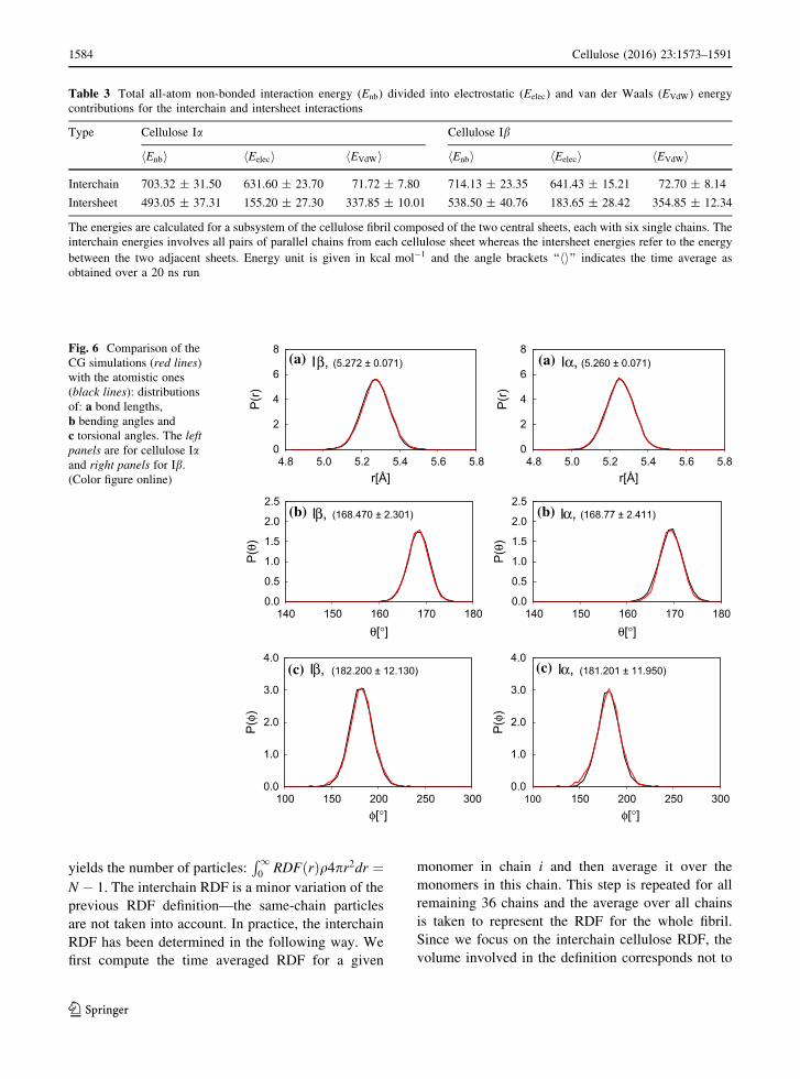
the CG approach works very well. Figure 6 indicates

that the distributions of the values of the bonded

degrees of freedom (r; h, and /) are essentially

identical, regardless of whether they are determined

during the CG (red lines) or all-atom (black lines)

evolutions. The distributions are Gaussian and their

means and dispersions are nearly the same for each of

the three degrees of freedom. In addition, the differ-

ences between the two allomorphs are small.

In order to characterize the type of packing in each

allomorph we have determined the RDF. For a system

of N interacting particles in a volume V, the RDF is

defined (Frenkel and Smit 2002; Allen and Tildesley

1993; Tuckerman 2010) as

RDFðrÞ ¼ hNðrÞihNidealðrÞi

ð5Þ

where r is the distance between a pair of particles. In

this equation, the numerator, hNðrÞi, is the average

number of particle pairs found between r and r þ dr.

The denominator is the average number of particles in

the same shell, assuming a fully random distribution at

density q ¼ N=V . This last quantity routinely can be

expressed as Nideal ¼ 4pðNpairs=VÞr2dr where Npairs ¼NðN � 1Þ (for non-distinguishable particles). Integrat-

ing the dimensionless RDF over the radial dependency

Table 1 Hydrogen bonds occupancy per D-GLC unit during

the MD simulation

Donor–acceptor Cellulose Ia Cellulose IbHB (%) HB (%)

Intrachaina

O3�H � � �O5 40.22 ± 3.32 43.52 ± 2.82

O2�H � � �O6 43.10 ± 3.41 46.52 ± 2.74

Inter-chaina

O6�H � � �O3 13.91 ± 2.73 14.34 ± 2.94

Intersheetb

C2�H � � �O4 4.11 ± 1.71 6.70 ± 1.34

C2�H � � �O3 3.01 ± 0.63 4.21 ± 0.72

C3�H � � �O2 1.30 ± 0.40 1.80 ± 0.32

C1�H � � �O6 2.40 ± 0.74 3.32 ± 0.61

C5�H � � �O3 1.71 ± 0.80 3.24 ± 0.73

C5�H � � �O4 1.01 ± 0.61 1.84 ± 0.44

The occupancy is defined as a fraction of the time that the bond

is found to be established. Situations with the occupancy

smaller than 1 % are not shown. The HBs are classified into

three main groups: intrachain HB, interchain HB, and

intersheet HB. The parameters for the HB analysis are as

follows: the distance ad(D-H � � �AÞ\3:0 A, the angle

\ðD-H � � �AÞ\20�; b d(D-H � � �AÞ\3:5 A, and the angle

\ðD-H � � �AÞ\30�

1582 Cellulose (2016) 23:1573–1591

123

Table 2 CG force field

parameters for the

allomorphs Ia and Ib in the

C4 representation

The top (bottom) part of the

table is for bonded (non-

bonded) interactions.

Entries for cellulose Ib are

cited after Ref. [Poma et al.

2015]. The Lennard-Jones

parameters eeff are derived

from the harmonic form of

the elastic potential near the

minimum of the potential

r C4

BI kr ðkcal/mol=A2Þ r0 ðAÞ EB kr ðkcal/mol=A

2Þ r0 ðAÞ

Cellulose Ia 119:2 � 3:7 5.258 103:3 � 14:1 5.262

OR cellulose Ib 120:3 � 4:3 5.248 104:2 � 14:3 5.266

CE cellulose Ib 120:1 � 4:1 5.252 102:1 � 15:0 5.279

h BI kh ðkcal/mol/rad2Þ h0 ð�Þ EB kh ð kcal/mol/rad2Þ h0 ð�Þ

Cellulose Ia 376:5 � 4:2 166.6 363:6 � 91:1 168.7

OR cellulose Ib 377:5 � 4:1 167.2 359:1 � 90:0 169.1

CE cellulose Ib 361:1 � 3:4 166.7 281:1 � 80:4 168.3

/ BI k/ ðkcal/mol/rad2Þ /0 ð�Þ EB k/ ð kcal/mol/rad2Þ /0 ð�Þ

Cellulose Ia 11:50 � 0:32 180.3 4:14 � 0:28 181.0

OR cellulose Ib 12:31 � 0:10 181.0 4:02 � 0:60 185.0

CE cellulose Ib 12:47 � 0:20 180.5 4:30 � 0:40 182.1

Non-

bonded

C4 reff ðAÞ

BI kr (kcal/mol=A2Þ eeff (kcal/mol) EB kr (kcal/mol=A

2Þ eeff (kcal/mol)

Cellulose Ib

Interchain

dOR4

48.13 46.62 7.660 7.410 7.440

dCE4

50.22 48.43 7.714 7.472 7.424

Intersheet

d1 24.01 12.23 3.803 1.941 5.400

d2 25.35 16.10 3.904 2.500 6.030

d5 24.40 12.10 4.751 2.360 5.327

d6 23.61 16.72 4.013 2.842 6.362

d7 27.83 12.60 4.610 2.082 5.080

d8 25.77 13.10 4.200 2.130 5.390

Inter-sheet�

d3 19.63 17.08 3.470 3.020 7.050

Cellulose Ia

Interchain

d4 37.25 36.57 7.411 7.280 7.490

Intersheet

d1 22.75 11.081 3.600 1.760 5.280

d2 20.13 13.61 3.321 2.250 6.220

d5 23.63 11.33 3.210 1.560 5.267

d6 19.23 10.40 3.704 2.004 5.560

d7 26.17 11.90 4.01 1.823 5.097

d8 16.83 12.91 2.460 1.900 6.620

Inter-sheet�

d3 18.01 15.02 3.104 2.590 6.904

Cellulose (2016) 23:1573–1591 1583

123

yields the number of particles:R1

0RDFðrÞq4pr2dr ¼

N � 1. The interchain RDF is a minor variation of the

previous RDF definition—the same-chain particles

are not taken into account. In practice, the interchain

RDF has been determined in the following way. We

first compute the time averaged RDF for a given

monomer in chain i and then average it over the

monomers in this chain. This step is repeated for all

remaining 36 chains and the average over all chains

is taken to represent the RDF for the whole fibril.

Since we focus on the interchain cellulose RDF, the

volume involved in the definition corresponds not to

Table 3 Total all-atom non-bonded interaction energy (Enb) divided into electrostatic (Eelec) and van der Waals (EVdW) energy

contributions for the interchain and intersheet interactions

Type Cellulose Ia Cellulose Ib

hEnbi hEeleci hEVdWi hEnbi hEeleci hEVdWi

Interchain 703.32 ± 31.50 631.60 ± 23.70 71.72 ± 7.80 714.13 ± 23.35 641.43 ± 15.21 72.70 ± 8.14

Intersheet 493.05 ± 37.31 155.20 ± 27.30 337.85 ± 10.01 538.50 ± 40.76 183.65 ± 28.42 354.85 ± 12.34

The energies are calculated for a subsystem of the cellulose fibril composed of the two central sheets, each with six single chains. The

interchain energies involves all pairs of parallel chains from each cellulose sheet whereas the intersheet energies refer to the energy

between the two adjacent sheets. Energy unit is given in kcal mol�1 and the angle brackets ‘‘hi’’ indicates the time average as

obtained over a 20 ns run

0

2

4

6

8

4.8 5.0 5.2 5.4 5.6 5.8

P(r

)

r[Å]

(a) Iβ, (5.272 ± 0.071)

0.0

0.5

1.0

1.5

2.0

2.5

140 150 160 170 180

P(θ

)

θ[°]

(b) Iβ, (168.470 ± 2.301)

0.0

1.0

2.0

3.0

4.0

100 150 200 250 300

P(φ

)

φ[°]

(c) Iβ, (182.200 ± 12.130)

0

2

4

6

8

4.8 5.0 5.2 5.4 5.6 5.8

P(r

)

r[Å]

(a) Iα, (5.260 ± 0.071)

0.0

0.5

1.0

1.5

2.0

2.5

140 150 160 170 180

P( θ

)

θ[°]

(b) Iα, (168.77 ± 2.411)

0.0

1.0

2.0

3.0

4.0

100 150 200 250 300

P(φ

)

φ[°]

(c) Iα, (181.201 ± 11.950)

Fig. 6 Comparison of the

CG simulations (red lines)

with the atomistic ones

(black lines): distributions

of: a bond lengths,

b bending angles and

c torsional angles. The left

panels are for cellulose Iaand right panels for Ib.

(Color figure online)

1584 Cellulose (2016) 23:1573–1591

123

the full simulational box but merely to the space

taken by the fibril (Lx ¼ 46:6 A; Ly ¼ 43:8 A; Lz ¼432:0 A for Ia and Lx ¼ 50:6 A; Ly ¼ 42:0 A; Lz ¼414:0 A for Ib). This is done both in the all-atom and

CG calculations. The all-atom results have been

shown in Fig. 2 and are now repeated in Fig. 7 to

make comparisons with the CG simulations. We have

performed two kinds of simulations. In the first kind,

the initial fiber structure was generated with the

cellulose-builder toolkit (Gomes and Skaf 2012) and

then energy minimized. In the second kind, as a

starting state we have used the snapshot obtained after

a 1 ns all-atom MD run. We observe that it is the

second CG kind that agrees very well with the all-atom

results. We interpret this as an evidence that important

conformational changes in the model fibril take place

as a result of the time evolution after the energy

minimization.

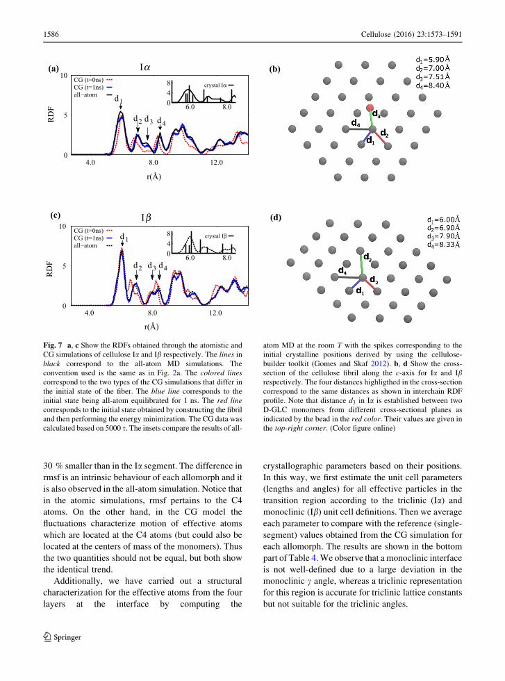
Additionally, the insets in Fig. 7a, c show the RDF

computed for the initial crystalline state. The line

pattern RDF corresponds to the ideal crystal structure

at zero temperature. Notice that the first peak for

crystalline Ia is represented by four single lines,

whereas for Ib only 3 lines contrinute to the same peak

at finite temperatures. This result shows that among

the four closest neighbours which contribute to the

first peak in crystal Ib, two of them are separated by

identical distances. The second peak is represented by

two lines, the third and fourth by a single line for each

of the allomorphs. At finite T’s the peaks broaden, shift

in position, and start to overlap.

These two allomorphs posses distinct unit cells and

hence different crystallographic parameters. Table 4

provides the experimental lattice parameters for Ia and

Ib allomorphs. The cellulose chains in Ib interact

through HBs in sheets parallel to the plane formed by

axes b and c (Fig. 1c) and are stacked in the direction

parallel to the vector b; the intersheet spacing between

two adjacent cellulose sheets is defined by D = a/2.

The experimental value for this parameter is 3.89 A at

room temperature. The organization of cellulose

chains in Ia is very similar to Ib: the chains are

parallel to the c-axis and sheets are grouped in parallel

layers. The experimental value for intersheet separa-

tion, D, is 3.91 A in Ia and 3.89 A in Ib. Table 4 shows

the lattice parameters computed with the CG model.

Our CG description was able to retain the difference in

D between the two allomorphs: it is 0.03 A instead of

0.02 A. In addition, the efficiency of our CG model

relative to all-atom simulations can be measured in

term of the cost required to reach a nanosecond time

scale when determining the RDF. We find that the CG

simulation is � 1000 times more efficient since it

takes half an hour compared to 500 h on the same

processor with the all-atom simulations.

Coexisting Ia and Ib regions in a cellulose fibril

Despite new advances in the understanding of the

cellulose biosynthesis in higher plants (Guerriero

et al. 2010; Harris et al. 2010; Li et al. 2014), it is

still unknown how cellulose chains assemble together

into fibrils. Explaining the coexistence ratios of Ia to

Ib in various plants appears to be even harder (Atalla

and VanderHart 1999; Fernandes et al. 2011). As an

example of this situation, we now consider a fiber

which is Ia on one end and Ib on another—see

Fig. 8a—with a transition region in between. The long

direction is taken to be along the c-axis. Numerical all-

atom simulations of such interfaces are often difficult

due to problems in setting up a well relaxed initial state

which would not lead to divergent atomic forces. Here,

we explore taking a CG-based approach. Its advantage

is that it allows for longer time scales necessary to

reach the relaxed state and the potentials involved are

soft.

We construct the initial configuration of the coex-

isting allomorphs via translation and alignment along

the c-axis of two separate fibrils Ia and Ib. Each fibril

is made of 36 D-GLC chains, 80-monomer long each.

The first 40 monomers are initially set in the MD-

relaxed Ia structure and the last 40—in the Ib one.

Note that this initial fibril structure is not realistic,

since the distance between monomers i and iþ 1 in

one chain at the interface is much larger than the

corresponding equilibrium distance in another.

We then assign specific CG potential parameters for

each allomorph in the two segments and evolve the

system until reaching a stationary state. The interface

acquires a transitional character which extends

between i of 39 and 42, as shown in Fig. 8. The lower

panel of this figure refers to the root mean square

fluctuations (rmsf) in the stationary state. They were

first calculated for each atom and then averaged over

cross-sectional planes corresponding to a given i. It is

seen that the fluctuations in the Ib segment are about

Cellulose (2016) 23:1573–1591 1585

123

30 % smaller than in the Ia segment. The difference in

rmsf is an intrinsic behaviour of each allomorph and it

is also observed in the all-atom simulation. Notice that

in the atomic simulations, rmsf pertains to the C4

atoms. On the other hand, in the CG model the

fluctuations characterize motion of effective atoms

which are located at the C4 atoms (but could also be

located at the centers of mass of the monomers). Thus

the two quantities should not be equal, but both show

the identical trend.

Additionally, we have carried out a structural

characterization for the effective atoms from the four

layers at the interface by computing the

crystallographic parameters based on their positions.

In this way, we first estimate the unit cell parameters

(lengths and angles) for all effective particles in the

transition region according to the triclinic (Ia) and

monoclinic (Ib) unit cell definitions. Then we average

each parameter to compare with the reference (single-

segment) values obtained from the CG simulation for

each allomorph. The results are shown in the bottom

part of Table 4. We observe that a monoclinic interface

is not well-defined due to a large deviation in the

monoclinic c angle, whereas a triclinic representation

for this region is accurate for triclinic lattice constants

but not suitable for the triclinic angles.

0

5

10

4.0 8.0 12.0

RD

F

r(Å)

d1

d2 d3 d4

CG (t=0ns) CG (t=1ns) all−atom

0 4 8

6.0 8.0

crystal Iα

(a) (b)

(d)

Iα

0

5

10

4.0 8.0 12.0

RD

F

r(Å)

d1

d2 d3 d4

CG (t=0ns) CG (t=1ns) all−atom

0 4 8

6.0 8.0

crystal Iβ

(c) Iβ

Fig. 7 a, c Show the RDFs obtained through the atomistic and

CG simulations of cellulose Ia and Ib respectively. The lines in

black correspond to the all-atom MD simulations. The

convention used is the same as in Fig. 2a. The colored lines

correspond to the two types of the CG simulations that differ in

the initial state of the fiber. The blue line corresponds to the

initial state being all-atom equilibrated for 1 ns. The red line

corresponds to the initial state obtained by constructing the fibril

and then performing the energy minimization. The CG data was

calculated based on 5000 s. The insets compare the results of all-

atom MD at the room T with the spikes corresponding to the

initial crystalline positions derived by using the cellulose-

builder toolkit (Gomes and Skaf 2012). b, d Show the cross-

section of the cellulose fibril along the c-axis for Ia and Ibrespectively. The four distances highligthed in the cross-section

correspond to the same distances as shown in interchain RDF

profile. Note that distance d3 in Ia is established between two

D-GLC monomers from different cross-sectional planes as

indicated by the bead in the red color. Their values are given in

the top-right corner. (Color figure online)

1586 Cellulose (2016) 23:1573–1591

123

Conversion of Ia to Ib at room temperature

The CG description allows for an easy determination

of the total potential energy of the two allomorphs in

the fibril form. We find that Ib is indeed lower in

energy than Ia. The energy difference in the stationary

state is DE ¼ hEai � hEbi ¼ 136:8 kcal/mol.

We now use the CG description to explore the

energy landscape corresponding to the transitions

between the two allomorphs at room temperature. We

induce the transition by first bringing an allomorph to

its equilibrium and then by switching the values of

non-bonded parameters eeff and reff to those corre-

sponding to the other allomorph, as listed in the

bottom part of Table 2. As a result, the system

overcomes high energy barriers that are normally

forbidden at room temperature. The energy changes

involved are shown in Fig. 9a. The parameters shown

in this figure were averaged over an ensemble of 100

induced trajectories for each system. Each trajectory

was divided into the following stages: the first 500 sprior the switching of CG parameters, then (2–6) scorresponding to the transition regime whose exact

duration depends on when all non-bonded interactions

(a)

Interface IβIα

Monomer Number

rmsf

[A]

454341393735

1.5

1.2

0.9

0.6

(b)

Fig. 8 a Snapshot of the interface between the Ia and Ibsegments of the fiber. The interface region is within the dashed

vertical lines and it comprises monomers 39 through 42. bshows the corresponding transition in the rmsf as a function of

the monomer number as calculated within the CG model (the

upper line) and the all-atom simulation (the horizontal segments

below). The average rmsf in CG simulation is 1.2 and 0.8 A for

the Ia and Ib segments respectively

Table 4 Lattice parameters for pure Ia (top) and Ib (middle) fibrils obtained from experiment, all-atom and CG simulation

Method V ðA3Þ a (A) b (A) c (A) a ð�Þ b ð�Þ c ð�Þ D (A)

Triclinic unit cell for cellulose Ia

Exp. ðT ¼ 295 KÞ 333.37 6.72 5.96 10.40 118.08 114.80 80.38 3.91

All-atom ðT ¼ 300 KÞ 339.73 6.82 5.95 10.43 118.11 114.35 80.48 3.98

CG 344.08 6.81 6.09 10.47 118.79 115.13 80.53 4.01

Monoclinic unit cell for cellulose Ib

Exp. ðT ¼ 295 KÞ 659.15 7.78 8.20 10.38 90 90 95.5 3.89

All-atom ðT ¼ 300 KÞ 679.62 7.90 8.34 10.43 89.92 90.11 98.51 3.95

CG 697.10 7.96 8.48 10.44 90.20 91.05 98.62 3.98

Unit cell j DV ðA3Þ j j Da ðAÞ j j Db ðAÞ j j Dc ðAÞ j j Da ð�Þ j j Db ð�Þ j j Dc ð�Þ j j DD ðAÞ j

Residues (39–42) at the interface

Triclinic 8.24 0.29 0.36 0.04 2.59 1.91 1.22 0.01

Monoclinic 20.65 0.05 0.05 0.07 0.33 0.25 7.12 0.03

The bottom table shows the absolute differences between crystallographic average values of the unit cell (triclinic or monoclinic)

computed for the particles at the interface and the reference CG values shown above. The difference of crystallographic parameters

between all-atom and CG simulations are within the error bars. For the lattice constants (a,b, and c) and the angles (a; b and c) are

about �0:2 and �1:80 respectively. Experimental data for cellulose Ia and Ib cited after refs. (Nishiyama et al. 2003) and (Nishiyama

et al. 2008) respectively

Cellulose (2016) 23:1573–1591 1587

123

(NBI) are recovered, and after that—500 s. The error

bar in the ground state energy of Ib for the transition

Ia ! Ib is 2.72 kcal/mol per trajectory and 1.80

kcal/mol in the ensemble of trajectories, hereas for Ia(in the reverse process Ib ! Ia) the corresponding

error bars are 3.92 kcal/mol per trajectory and 2.40

kcal/mol in the ensemble. The single-trajectory error

bars are comparable to those of the ensamble-averaged

data which reflects existence of correlations induced

by the adoption of the same crystalline initial state.

Notice that the NBI in equilibrium is equal to 12861

for both allomorphs. To determine the transition state

(TS) the change in the NBI in the parameter-switching

trajectories. In this way, the TS state is uniquely

defined by the minimum value of NBI on the pathway.

In practice, a trajectory starts by first losing some of its

initial NBIs. Note that the system has to go through

high energy conformations in order to reach the final

destination. We have verified that the simulation

reached the final state compatible with the CG

parameters by computing the interchain RDF for the

final structure (data not shown). The TS for the Ib !Ia transition has a higher energy and a smaller number

of NBIs than for the reverse transition. Panels (b) and

(c) in Fig. 9 show examples of snapshots of the TS for

the two processes.

For the Ia ! Ib process the TS is characterized by a

loss of about 5 % of the initial NBI. The reverse

process Ib ! Ia leads to a TS characterized by twice

the loss of about 10 % of the initial NBIs. Such losses

affects packing of the chains and gives raise to

amorphous regions across the fibril structure. Further-

more, by computing the time needed to go over the

energy barrier, we find that a longer escaping time is

needed to implement the process Ib ! Ia(tb!a � 2ta!b). This is consistent with Ib having a

lower free energy than Ia.

We now assess the difference in the free energy

between the CG representations of the two allomorphs

by using the thermodynamic integration (TI) approach

(Frenkel and Smit 2002). In TI, a hybrid potential

function (Uhyb) is defined as follows:

Fig. 9 a The energy landscape for the convertion process

between Ia and Ib as derived through the CG simulations. The

energies are given in units of kcal/mol and conversion times in

unit of s (of order 1 ns). The numbers of non-bonded

interactions (NBI) are indicated. The pure state energies were

averaged in 100 trajectories for 500 s before switching the CG

parameters to another phase. The error bars for the average

energies, hEai and hEbi are 2.40 kcal/mol and 1.80 kcal/mol

respectively. The error bars in the transition state energies are

30.4 kcal/mol for the Ia ! Ib process and 45.6 for the reverse

process. b and c show examples of snapshots of the transition

state (TS) found for the conversion process Ia ! Ib and its

reverse respectively

1588 Cellulose (2016) 23:1573–1591

123

UhybðkÞ ¼ kUa þ 1 � kð ÞUb; ð6Þ

where k is a coupling parameter. This parameter

indicates the level of change that is taking place on

switching between Ia and Ib. The potential Ua and Ub

correspond here to the CG energies of the two

allomorphs respectively. The interactions are switched

when k is continuously decreased. Simulations con-

ducted at different values of k allow to plot aoUðkÞok

curve, from which DF ¼ Fa � Fb is derived as below:

Fa � Fb ¼Z 1

0

oUhybðkÞok

� �

k

dk; ð7Þ

where Uhyb is the hybrid interaction and h�i denotes the

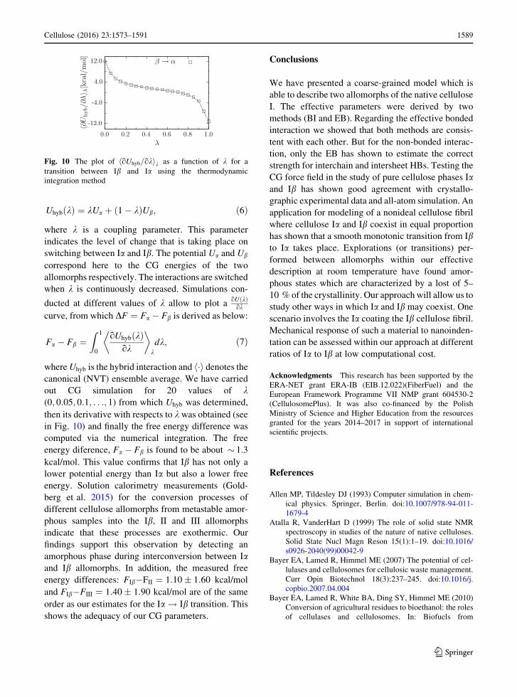
canonical (NVT) ensemble average. We have carried

out CG simulation for 20 values of k(0; 0:05; 0:1; . . .; 1) from which Uhyb was determined,

then its derivative with respects to k was obtained (see

in Fig. 10) and finally the free energy difference was

computed via the numerical integration. The free

energy diference, Fa � Fb is found to be about � 1.3

kcal/mol. This value confirms that Ib has not only a

lower potential energy than Ia but also a lower free

energy. Solution calorimetry measurements (Gold-

berg et al. 2015) for the conversion processes of

different cellulose allomorphs from metastable amor-

phous samples into the Ib, II and III allomorphs

indicate that these processes are exothermic. Our

findings support this observation by detecting an

amorphous phase during interconversion between Iaand Ib allomorphs. In addition, the measured free

energy differences: FIb�FII ¼ 1:10 � 1:60 kcal/mol

and FIb�FIII ¼ 1:40 � 1:90 kcal/mol are of the same

order as our estimates for the Ia ! Ib transition. This

shows the adequacy of our CG parameters.

Conclusions

We have presented a coarse-grained model which is

able to describe two allomorphs of the native cellulose

I. The effective parameters were derived by two

methods (BI and EB). Regarding the effective bonded

interaction we showed that both methods are consis-

tent with each other. But for the non-bonded interac-

tion, only the EB has shown to estimate the correct

strength for interchain and intersheet HBs. Testing the

CG force field in the study of pure cellulose phases Iaand Ib has shown good agreement with crystallo-

graphic experimental data and all-atom simulation. An

application for modeling of a nonideal cellulose fibril

where cellulose Ia and Ib coexist in equal proportion

has shown that a smooth monotonic transition from Ibto Ia takes place. Explorations (or transitions) per-

formed between allomorphs within our effective

description at room temperature have found amor-

phous states which are characterized by a lost of 5–

10 % of the crystallinity. Our approach will allow us to

study other ways in which Ia and Ib may coexist. One

scenario involves the Ia coating the Ib cellulose fibril.

Mechanical response of such a material to nanoinden-

tation can be assessed within our approach at different

ratios of Ia to Ib at low computational cost.

Acknowledgments This research has been supported by the

ERA-NET grant ERA-IB (EIB.12.022)(FiberFuel) and the

European Framework Programme VII NMP grant 604530-2

(CellulosomePlus). It was also co-financed by the Polish

Ministry of Science and Higher Education from the resources

granted for the years 2014–2017 in support of international

scientific projects.

References

Allen MP, Tildesley DJ (1993) Computer simulation in chem-

ical physics. Springer, Berlin. doi:10.1007/978-94-011-

1679-4

Atalla R, VanderHart D (1999) The role of solid state NMR

spectroscopy in studies of the nature of native celluloses.

Solid State Nucl Magn Reson 15(1):1–19. doi:10.1016/

s0926-2040(99)00042-9

Bayer EA, Lamed R, Himmel ME (2007) The potential of cel-

lulases and cellulosomes for cellulosic waste management.

Curr Opin Biotechnol 18(3):237–245. doi:10.1016/j.

copbio.2007.04.004

Bayer EA, Lamed R, White BA, Ding SY, Himmel ME (2010)

Conversion of agricultural residues to bioethanol: the roles

of cellulases and cellulosomes. In: Biofuels from

λ

∂U

hyb/∂λ

λ[kcal/mol]

1.00.80.60.40.20.0

12.0

4.0

-4.0

-12.0

β → α

Fig. 10 The plot of hoUhyb=okik as a function of k for a

transition between Ib and Ia using the thermodynamic

integration method

Cellulose (2016) 23:1573–1591 1589

123

agricultural wastes and byproducts, Wiley-Blackwell,

pp 67–96, doi:10.1002/9780813822716.ch5

Bellesia G, Chundawat SPS, Langan P, Redondo A, Dale BE,

Gnanakaran S (2012) Coarse-grained model for the inter-

conversion between native and liquid ammonia-treated

crystalline cellulose. J Phys Chem B 116(28):8031–8037.

doi:10.1021/jp300354q

Bu L, Himmel ME, Nimlos MR (2010) Meso-scale modeling of

polysaccharides in plant cell walls: an application to

translation of CBMs on the cellulose surface. In: ACS

symposium series, American Chemical Society (ACS),

pp 99–117, doi:10.1021/bk-2010-1052.ch005

Darden T, York D, Pedersen L (1993) Particle mesh ewald: an

n � log(n) method for ewald sums in large systems.

J Chem Phys 98(12):10,089. doi:10.1063/1.464397

Dashtban M (2009) Fungal bioconversion of lignocellulosic

residues; opportunities & perspectives. Int J Biol Sci

pp 578–595, doi:10.7150/ijbs.5.578

Debzi EM, Chanzy H, Sugiyama J, Tekely P, Excoffier G (1991)

The Ialpha ! Ibeta transformation of highly crystalline

cellulose by annealing in various mediums. Macro-

molecules 24(26):6816–6822. doi:10.1021/ma00026a002

Ding SY, Himmel ME (2006) The maize primary cell wall

microfibril: a new model derived from direct visualization.

J Agric Food Chem 54(3):597–606. doi:10.1021/jf051851z

Eadie L, Ghosh TK (2011) Biomimicry in textiles: past, present

and potential. An overview. J R Soc Interface 8(59):761–

775. doi:10.1098/rsif.2010.0487

Fan B, Maranas JK (2014) Coarse-grained simulation of cellu-

lose Ib with application to long fibrils. Cellulose

22(1):31–44. doi:10.1007/s10570-014-0481-2

Fernandes AN, Thomas LH, Altaner CM, Callow P, Forsyth VT,

Apperley DC, Kennedy CJ, Jarvis MC (2011) Nanostructure

of cellulose microfibrils in spruce wood. Proc Natl Acad Sci

108(47):E1195–E1203. doi:10.1073/pnas.1108942108

Foston M, Ragauskas AJ (2010) Changes in lignocellulosic

supramolecular and ultrastructure during dilute acid pre-

treatment of populus and switchgrass. Biomass Bioenerg

34(12):1885–1895. doi:10.1016/j.biombioe.2010.07.023

Frenkel D, Smit B (2002) Understanding Molecular Simula-

tion. Academic Press. doi:10.1016/b978-012267351-1/

50006-7

Goldberg RN, Schliesser J, Mittal A, Decker SR, Santos AFL,

Freitas VL, Urbas A, Lang BE, Heiss C, da Silva MDR,

Woodfield BF, Katahira R, Wang W, Johnson DK (2015) A

thermodynamic investigation of the cellulose allomorphs:

Cellulose(am), cellulose Ib(cr), cellulose II(cr), and cel-

lulose III(cr). J Chem Thermodyn 81:184–226. doi:10.

1016/j.jct.2014.09.006

Gomes TCF, Skaf MS (2012) Cellulose-builder: a toolkit for

building crystalline structures of cellulose. J Comput Chem

33(14):1338–1346. doi:10.1002/jcc.22959

Guerriero G, Fugelstad J, Bulone V (2010) What do we really

know about cellulose biosynthesis in higher plants? J Integr

Plant Biol 52(2):161–175. doi:10.1111/j.1744-7909.2010.

00935.x

Hakansson KMO, Fall AB, Lundell F, Yu S, Krywka C, Roth

SV, Santoro G, Kvick M, Wittberg LP, Wagberg L, Sder-

berg LD (2014) Hydrodynamic alignment and assembly of

nanofibrils resulting in strong cellulose filaments. Nat

Commun 5. doi:10.1038/ncomms5018

Hardy BJ, Sarko A (1996) Molecular dynamics simulations and

diffraction-based analysis of the native cellulose fibre:

structural modelling of the I-a and I-b phases and their

interconversion. Polymer 37(10):1833–1839. doi:10.1016/

0032-3861(96)87299-5

Harris D, Bulone V, Ding SY, DeBolt S (2010) Tools for cel-

lulose analysis in plant cell walls. Plant Physiol

153(2):420–426. doi:10.1104/pp.110.154203

Heiner AP, Sugiyama J, Teleman O (1995) Crystalline cellulose

Ialpha and Ibeta studied by molecular dynamics simula-

tion. Carbohydr Res 273(2):207–223. doi:10.1016/0008-

6215(95)00103-z

Humphrey W, Dalke A, Schulten K (1996) VMD: visual

molecular dynamics. J Mol Graph 14(1):33–38. doi:10.

1016/0263-7855(96)00018-5

Imai T, Sugiyama J, Itoh T, Horii F (1999) Almost pure I(alpha)

cellulose in the cell wall of glaucocystis. J Struct Biol

127(3):248–257. doi:10.1006/jsbi.1999.4160

Jarvis MC (2000) Interconversion of the Ia and Ib crystalline

forms of cellulose by bending. Carbohydr Res

325(2):150–154. doi:10.1016/s0008-6215(99)00316-x

Jochum M, Andrienko D, Kremer K, Peter C (2012) Structure-

based coarse-graining in liquid slabs. J Chem Phys

137(6):064,102. doi:10.1063/1.4742067

Jorgensen WL, Chandrasekhar J, Madura JD, Impey RW, Klein

ML (1983) Comparison of simple potential functions for

simulating liquid water. J Chem Phys 79(2):926. doi:10.

1063/1.445869

Kataoka Y, Kondo T (1999) Quantitative analysis for the cel-

lulose I alpha crystalline phase in developing wood cell

walls. Int J Biol Macromol 24(1):37–41. doi:10.1016/

s0141-8130(98)00065-8

Kirschner KN, Yongye AB, Tschampel SM, Gonzalez-Out-

eirino J, Daniels CR, Foley BL, Woods RJ (2008) GLY-

CAM06: a generalizable biomolecular force field.

carbohydrates. J Comput Chem 29(4):622–655. doi:10.

1002/jcc.20820

Kroon-Batenburg LMJ, Bouma B, Kroon J (1996) Stability of

cellulose structures studied by MD simulations. Could

mercerized cellulose II be parallel? Macromolecules

29(17):5695–5699. doi:10.1021/ma9518058

Lee KY, Buldum G, Mantalaris A, Bismarck A (2013) More

than meets the eye in bacterial cellulose: biosynthesis,

bioprocessing, and applications in advanced fiber com-

posites. Macromol Biosci 14(1):10–32. doi:10.1002/mabi.

201300298

Lee KY, Aitomki Y, Berglund LA, Oksman K, Bismarck A

(2014) On the use of nanocellulose as reinforcement in

polymer matrix composites. Compos Sci Technol

105:15–27. doi:10.1016/j.compscitech.2014.08.032

Li S, Bashline L, Lei L, Gu Y (2014) Cellulose synthesis and its

regulation. Arabid Book 12:e0169. doi:10.1199/tab.0169

Lin N, Dufresne A (2014) Nanocellulose in biomedicine: cur-

rent status and future prospect. Eur Poly J 59:302–325.

doi:10.1016/j.eurpolymj.2014.07.025

Lopez CA, Bellesia G, Redondo A, Langan P, Chundawat SPS,

Dale BE, Marrink SJ, Gnanakaran S (2015) MARTINI

coarse-grained model for crystalline cellulose microfibers.

J Phys Chem B 119(2):465–473. doi:10.1021/jp5105938

Martonak R, Laio A, Bernasconi M, Ceriani C, Raiteri P, Zipoli

F, Parrinello M (2005) Simulation of structural phase

1590 Cellulose (2016) 23:1573–1591

123

transitions by metadynamics. Zeitschrift fr Kristallogra-

phie—Cryst Mater 220(5/6). doi:10.1524/zkri.220.5.489.

65078

Matthews JF, Himmel ME, Crowley MF (2011) Conversion of

cellulose Ia to Ib via a high temperature intermediate (i-

HT) and other cellulose phase transformations. Cellulose

19(1):297–306. doi:10.1007/s10570-011-9608-x

Meyer H, Biermann O, Faller R, Reith D, Muller-Plathe F

(2000) Coarse graining of nonbonded inter-particle

potentials using automatic simplex optimization to fit

structural properties. J Chem Phys 113(15):6264. doi:10.

1063/1.1308542

Mihranyan A, Edsman K, Strømme M (2007) Rheological

properties of cellulose hydrogels prepared from cladophora

cellulose powder. Food Hydrocoll 21(2):267–272. doi:10.

1016/j.foodhyd.2006.04.003

Molinero V, Goddard WA (2004) M3b: a coarse grain force field

for molecular simulations of malto-oligosaccharides and

their water mixtures. J Phys Chem B 108(4):1414–1427.

doi:10.1021/jp0354752

Nawrath C, Poirier Y, Somerville C (1995) Plant polymers for

biodegradable plastics: cellulose, starch and polyhydrox-

yalkanoates. Mol Breed 1(2):105–122. doi:10.1007/

bf01249696

Newman RH (1999) Estimation of the relative proportions of

cellulose I alpha and I beta in wood by carbon-13 NMR

spectroscopy. Holzforschung 53(4). doi:10.1515/hf.1999.

055

Nishiyama Y, Langan P, Chanzy H (2002) Crystal structure and

hydrogen-bonding system in cellulose Ibeta from syn-

chrotron X-ray and neutron fiber diffraction. J Am Chem

Soc 124(31):9074–9082. doi:10.1021/ja0257319

Nishiyama Y, Sugiyama J, Chanzy H, Langan P (2003) Crystal

structure and hydrogen bonding system in cellulose I(al-

pha) from synchrotron X-ray and neutron fiber diffraction.

J Am Chem Soc 125(47):14,300–14,306. doi:10.1021/

ja037055w

Nishiyama Y, Johnson GP, French AD, Forsyth VT, Langan P

(2008) Neutron crystallography, molecular dynamics, and

quantum mechanics studies of the nature of hydrogen

bonding in cellulose Ibeta. Biomacromolecules

9(11):3133–3140. doi:10.1021/bm800726v

Peplow M (2014) Cellulosic ethanol fights for life. Nature

507(7491):152–153. doi:10.1038/507152a

Phillips JC, Braun R, Wang W, Gumbart J, Tajkhorshid E, Villa

E, Chipot C, Skeel RD, Kale L, Schulten K (2005) Scalable

molecular dynamics with NAMD. J Comput Chem

26(16):1781–1802. doi:10.1002/jcc.20289

Poma AB, Chwastyk M, Cieplak M (2015) Polysaccharide–

protein complexes in a coarse-grained model. J Phys Chem

B 119(36):12,028–12,041. doi:10.1021/acs.jpcb.5b06141

Queyroy S, Neyertz S, Brown D, Mller-Plathe F (2004)

Preparing relaxed systems of amorphous polymers by

multiscale simulation: application to cellulose. Macro-

molecules 37(19):7338–7350. doi:10.1021/ma035821d

Revol JF (1982) On the cross-sectional shape of cellulose

crystallites in valonia ventricosa. Carbohydr Polym

2(2):123–134. doi:10.1016/0144-8617(82)90058-3

Sannigrahi P, Ragauskas AJ, Miller SJ (2008) Effects of two-

stage dilute acid pretreatment on the structure and com-

position of lignin and cellulose in loblolly pine. BioEnerg

Res 1(3–4):205–214. doi:10.1007/s12155-008-9021-y

Sassi JF, Tekely P, Chanzy H (2000) Relative susceptibility of

the Ia and Ib phases of cellulose towards acetylation.

Cellulose 7:119–132. doi:10.1023/A:1009224008802

Sikora M, Sułkowska JI, Cieplak M (2009) Mechanical strength

of 17 134 model proteins and cysteine slipknots. PLoS

Comput Biol 5(21000):547. doi:10.1371/journal.pcbi.

1000547

Srinivas G, Cheng X, Smith JC (2014) Coarse-grain model for

natural cellulose fibrils in explicit water. J Phys Chem B

118(11):3026–3034. doi:10.1021/jp407953p

Steiner T (2002) The hydrogen bond in the solid state. Angew

Chem Int 41(1):48–76. doi:10.1002/1521-3773

Sułkowska JI, Cieplak M (2007) Mechanical stretching of pro-

teins—a theoretical survey of the protein data bank. J Phys:

Cond Matter 19(285):224

Tessier M, DeMarco M, Yongye A, Woods R (2008) Extension

of the GLYCAM06 biomolecular force field to lipids, lipid

bilayers and glycolipids. Mol Simul 34(4):349–364.

doi:10.1080/08927020701710890

Tuckerman ME (2010) Statistical mechanics: theory andmolecular simulation. Oxford University Press, Oxford.

doi:10.1016/b978-012267351-1/50006-7

Vashchenko AV, Afonin AV (2014) A study of intramolecular

hydrogen bonds C-H � � �X (X = N, O) within the the-

ory of the electron localization function. J Struct Chem

55(6):1010–1018. doi:10.1134/s002247661406002x

Wada M, Kondo T, Okano T (2003) Thermally induced crystal

transformation from cellulose Ia to Ib. Polym J

35(2):155–159. doi:10.1295/polymj.35.155

Wertz JL, Mercier JP, Bedue O (2010) Cellulose science and

technology. Informa UK Limited, London. doi:10.1201/

b16496

Wohlert J, Berglund LA (2011) A coarse-grained model for

molecular dynamics simulations of native cellulose.

J Chem Theory Comput 7(3):753–760. doi:10.1021/

ct100489z

Wu X, Moon RJ, Martini A (2014) Tensile strength of Ibeta

crystalline cellulose predicted by molecular dynamics

simulation. Cellulose 21(4):2233–2245. doi:10.1007/

s10570-014-0325-0

Yu TQ, Chen PY, Chen M, Samanta A, Vanden-Eijnden E,

Tuckerman M (2014) Order-parameter-aided temperature-

accelerated sampling for the exploration of crystal poly-

morphism and solid-liquid phase transitions. J Chem Phys

140(21):214,109. doi:10.1063/1.4878665

Cellulose (2016) 23:1573–1591 1591

123