coarse grained stochastic birth-death processes for ... · coarse grained stochastic birth-death...

1

Coarse Grained StochasticBirth-Death Processes forTropical Convection and

Climate

B. KhouiderUniversity of Victoria

Summer School on stochastic and probabilistic methods, UVic

14-18, 2008

2

OUTLINE• Part I:

– Introduction, unresolved features (CAPE and CIN)

– Stochastic spin/flip model and coarse-graining

– Deterministic model and coupling

– Walker cell simulations: stochastic effect on climate

– Summary

• Part II: (Aquaplanet setup)

– Mean field/Stochastic RCE’s

– Selecting stochastic regimes and RCEs

– Intermittency in single column

– Effect of CIN on deep convective activity and convectively

coupled waves

• Conclusion

3

Relevant papers

• Atmospheric science:

Majda, Franzke, & Khouider, (2008), Phyl. Trans.: Applied

math perspective on stochastic modeling for climate

Khouider, Majda, & Katsoulakis (2003), PNAS: Coarse grained

stochastic models for tropical convection and climate.

Majda & Khouider (2002), PNAS: Stochastic and mesoscopic

models for tropical convections.

• Theory

Katsoulakis, Majda, & Vlachos , JCP(2003) and PNAS (2003),

(material science, coarse graining)

Katsoulakis, Majda, & Sopasakis (2004, 2005a, 2005b):

Multiscale Coupling, Intermittency, metastability, and phase

transition

4

Introduction

• Moist convection: Transport of latent heat.

• Source of energy for local and large scale circulation.

• Generates and maintains tropical waves and storms.

• Organized tropical convection ranges from mesoscale individual

clouds (1-10 km) to large scale superclusters (1000-10,000 km).

• Poorly represented by GCM’s despite Today’s supercomputers.

• Major contemporary problem: How large-scale circulation

supplies energy and maintains deep convection?

• Convective Inhibition (CIN): Energy Barrier for spontaneous

convection

5

Motivation

• Can Stochastic parametrizations alter tropical Climatology?

• Can they increase the wave fluctuations?

• Lin & Neelin: suggest plausible influence of stochastic

convective parametrizations on the variability in GCM’s.

6

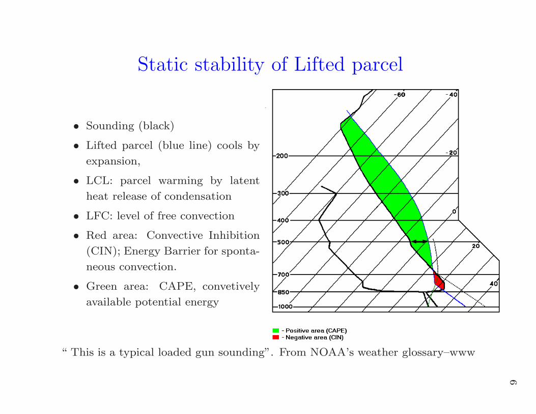
Static stability of Lifted parcel

• Sounding (black)

• Lifted parcel (blue line) cools by

expansion,

• LCL: parcel warming by latent

heat release of condensation

• LFC: level of free convection

• Red area: Convective Inhibition

(CIN); Energy Barrier for sponta-

neous convection.

• Green area: CAPE, convetively

available potential energy

“ This is a typical loaded gun sounding”. From NOAA’s weather glossary–www

7

• (Thermal) Buoyancy of a lifted parcel:

B = gθe,p − θe,a

θe,a

θe = temperature + moisture content × latent heat

• Potential energy of lifted parcel

Ep =

∫ LNB

0

gθe,p − θe,a

θe,adz

=

∫ LFC

0

—- dz +

∫ LNB

LFC

—- dz

= −CIN + CAPE

• When (how) parcel has (could have) enough energy to

overcome CIN and reach LFC?

8

Microscopic stochastic Model for CIN

• CIN: Energy Barrier for spontaneous convection

• Observationally, factors for CIN complex:gust fronts, gravity waves, density currents, turbulent

fluctuations in boundary layer equivalent potential

temperature, etc.

• Too complex to model in detail; instead, borrow ideas from

statistical physics and material science of representing these

effects by an order parameter, σI

9

• Order parameter, σI , sites (1-10 km apart)

σI = 1 if deep convection is inhibited: a CIN site

σI = 0 if there is potential for deep convection: a PAC site

Sigma_I = 1 Sigma_I = 1 Sigma_I = 0

10

• Coarse Mesh: Average CIN

j∆x, ∆x = O(100, 200 km) (mesoscopic scale)

σI(j∆x, t) =1

∆x

∫ (j+1/2)∆x

(j−1/2)∆x

σI(x, t) dx

100−200 km

j Delta X

11

Intuitive Stochastic Rules for Interaction ofOrder Parameter, σI

A) If CIN site is surrounded mostly by CIN sites, should remain so

with high probability

B) If PAC site is surrounded by CIN sites, should have high

probability to switch to CIN site

C) The external large scale mesoscopic mesh values, ~uj , should

supply external potential, h(~uj), which modifies dynamics in

A) and B) according to whether external conditions favor CIN

or PAC

12

Stochastic Model• View boundary layer as heat bath with external Potential:

Ising model (magnetization and phase transition)

Materials science: Souganidis, Katsoulakis, etc.

• Microscopic energy for CIN:

Hh(σI) =∑

x6=y

J(|x − y|

L)σI(x)σI(y) + h

∑

x

σI(x)

– J : microscopic interaction potential: (Currie-Weiss)

J(r) =

U0, r < r0

0, r > r0

– h: external potential. Hh ր h

• Invariant Gibbs measure: G = (ZΛ)−1 exp[βHh(σ)]dσ

ZΛ : partition function.

13

• Spin flip rule: σxI (y) =

1 − σI(x), y = x

σI(y), y 6= x

• Arrhenius dynamics:

Rate: c(x, σI) =

τ−1 exp[−βV (x)], x = 1

τ−1, x = 0

V (x) ≡ ∆H =∑

z 6=x

J(x − z)σI + h(x) (detailed balance)

τI : CIN characteristic time O(days)

• With U0 > 0: if a CIN site is mostly surrounded by CIN sites,

then it needs to overcome a larger energy barrier.

• External field also builds/destroys energy for CIN: Hh ր h

14

Coarse-Graining

• Coarse-grained stochastic process:

ηt(k) =∑

x∈Dk

σI,t(x); η(k) ∈ {0, 1, · · · , q}

average CIN on coarse-mesh: σI [Dk] =1

qη(k)

Dk

x

15

Features of coarse-grained process

• Canonical invariant Gibbs measure:

Gm,q,β(η) = 1Zm,q,β

eβH(η)Pm,q(dη)

• Coarse grained Hamiltonian

H(η) = U0

q−1

∑

l∈Λc

η(l)(

η(l) − 1)

+ h∑

l∈Λc

η(l)

• Arrhenius Dynamics lead to birth/death process with

Adsorption/Desorption rates:

Ca(k, n) =1

τI[q − η(k)]

Cd(k, n) =1

τIη(k)e−βV (k)

with V (η) = ∆H(η) =2U0

q − 1

(

η(k) − 1)

+ h

16

Stochastic model for CIN coupled into aone-and-half layer model convectiveparametrization (toy GCM)

��

��

��

��

High precipitation

Hot tower

Planetary Boundary Layer500 m

16 km

SEA SURFACE

< 10 km

cumulus cloud with anvil top

17

The Deterministic Model (Toy GCM): model

convective parametrization

• Prognostic Eqns: One vertical baroclinic mode, no rotation

∂u

∂t− ¯α

∂θ

∂x= −Friction

∂θ

∂t− α

∂u

∂x= Qc − QR

h∂θeb

∂t= −D + E H

∂θem

∂t= D − QR

Convective heating:

Qc = Mσc

(

(CAPE)+)1/2

CAPE ∝ θeb − γθ.

σc called area fraction of deep convection, plays key role in linear

stability.

18

Coupling Stochastic model into toy GCM

• Order parameter modifies CAPE flux:

σc = (1 − σI)σ+c ; σ+

c = .002

• External potential depends on large scale dynamics and

thermodynamics: (Good guess)

h ∝ m−,

Downward mass flux ∝ Convective mass flux

• convective events build CIN by downdraft cooling of boundary

layer and/or convective heating of middle troposphere

(stabilization)

• Other choices of h are also considered (Part 2).

19

Nonlinear Simulations with Toy GCMWalker circulation set-up:

mimicking the Indian Ocean/Western Pacific warm poolθ∗

eb(x)

θ∗,0eb

= 1 + A0 cos(π(x−x0)

L0

)

, |x − x0| < L0

2

0 5 10 15 20 25 30 35 400

2

4

6

8

10

12

14

16

18

20

Equator (40,000 km)

θ* eb(K)

θ*eb

(x)

• Periodic geometry, ∆x = 80 km

• Initial data: RCE + small random perturbation

• Integrate to statistical equilibrium

• Effects of stochastic model on waves and climate?

• Vary stochastic parameters, βU0, τI , and A0

20

Table 1: Effect of stochastic parameters on climatology and fluctua-

tions, with heating strength A0 = .5.

Interac.

pot.τI (m s−1)

Std.

Dev.

βU0 (days) u− u+ u′

−u′

+σc

1 5 −.856 .855 −.207 .214 4.55E−04 3.00E−04

1 20 −.855 .856 −.214 .208 4.55E−04 2.96E−04

.01 5 −1.047 1.046 −.508 .486 9.96E−04 3.18E−04

.01 20 −1.048 1.040 −.804 .676 9.96E−04 3.15E−04

−.01 5 −1.047 1.049 −.603 .572 1.00E−03 3.15E−04

−.01 10 −.923 .920 −4.497 4.429 1.00E−03 3.14E−04

−.1 5 −.816 .867 −4.820 4.727 1.04E−03 3.11E−04

−.1 10 −.824 .877 −4.861 4.737 1.04E−03 3.12E−04

21

Table 2: Same as in Table 1, except for A0 = 1.

Interac.

pot.τI (m s−1)

Std.

Dev.

βU0 (days) u− u+ u′

−u′

+σc

1 5 −1.417 1.417 −.536 .436 4.56E−04 3.00E−04

1 20 −1.415 1.417 −.330 .546 4.56E−04 3.00E−04

.01 5 −1.692 1.691 −1.196 1.603 9.96E−04 3.17E−04

.01 20 −1.692 1.691 −1.180 1.266 9.96E−04 3.17E−04

−.01 5 −1.693 1.693 −1.421 1.470 1.00E−03 3.15E−04

−.01 10 −1.693 1.693 −1.277 1.243 1.00E−03 3.16E−04

−.1 5 −1.700 1.699 −.990 1.092 1.04E−03 3.10E−04

−.1 10 −1.700 1.700 −1.447 1.269 1.04E−03 3.07E−04

22

Typical case: βU0 = 1, τI = 20 days, A0 = .5

0 10000 20000 30000 400000

3

6

9

12

Hei

ght,

km

Contour Interval: .3 K day−1; Max arrow: .85 m s−1; Max w: .18 cm s−1

Equator, km

23

0 10000 20000 30000 40000−1

−0.5

0

0.5

1U

(m

/s)

0 10000 20000 30000 400008

8.5

9

9.5

10

10.5x 10

−3

Wat

er V

apor

24

PAC favor-

ing but small

CIN time:

βU0 = −.01,

τI = 5 days,

A0 = .5

0 10000 20000 30000 40000−1.5

−1

−0.5

0

0.5

1

1.5

U (

m/s

)

0 10000 20000 30000 400008

8.5

9

9.5

10x 10

−3

Wat

er V

apor

25

PAC favor-

ing with

larger CIN

time:

βU0 = −.01,

τI = 10

days,

A0 = .5

0 10000 20000 30000 40000−1.5

−1

−0.5

0

0.5

1

1.5

U (

m/s

)

0 10000 20000 30000 400008

8.5

9

9.5

10x 10

−3

Wat

er V

apor

26

−6

−5

−4

−3

−2

−1

0

1

2

3

4

0 5 10 15 20 25 30 35360

365

370

375

380

385

390

395

Equator (40,000 km)

Tim

e (d

ays)

Walker cell set up: CWV, With WISHE, ENO OFF,detrministic: σcd

=.001, ∆ x=80 km, u0=2 m/s, A

0=.5,µ=0

Constant area fraction: σc = .001, A0 = .5

27

−0.6

−0.5

−0.4

−0.3

−0.2

−0.1

0

0.1

0.2

0.3

0.4

0 5 10 15 20 25 30 35260

265

270

275

280

285

290

295

Equator (40,000 km)

Tim

e (d

ays)

Walker cell set up: CWV, With WISHE, ENO OFF,σc+=.002, ∆ x=80 km, u

0=2 m/s, A

0=.5,\tau

I=5 days,beta J

0=−.01,

βU0 = −.01, τI = 5 days, A0 = .5 (σc = .001)

28

−4

−3

−2

−1

0

1

2

3

4

0 5 10 15 20 25 30 35260

265

270

275

280

285

290

295

Equator (40,000 km)

Tim

e (d

ays)

Walker cell set up: CWV, With WISHE, ENO OFF,σc+=.002, ∆ x=80 km, u

0=2 m/s, A

0=.5,τ

I=10 days,beta J

0=−.01,

βU0 = −.01, τI = 10 days, A0 = .5 (σc = .001)

29

• Strong forcing (A0 = 1): Walker cell climatology + weak

gravity waves (except for deterministic case)

• Moderate forcing (A0 = .5):

– Deterministic case: one large scale wave propagating around

globe, no Walker cell

– CIN favoring interaction potential (βU0 > 0): Walker cell

forms + moderate small scale squall line-like waves

– As interaction potential decreases strength and length scale

of convective waves increases

– Also sensitive to CIN charac. time (τI)

– PAC favoring int. pot. (βU0 < 0): Walker cell destroyed

and two symmetric waves propagating far from source

• Stochastic (noise) creates and maintains Walker cell and

• Affects wavelength and strength of waves

30

Mean field/Stochastic RCE’s

• Large scale variable equations

∂v

∂t−

∂θ

∂x= −

Cd(u0)

hbv −

1

τDv

∂θ

∂t−

∂v

∂x= Qc − Q0

R −1

τRθ

∂θeb

∂t= −

1

τebD(θeb − θem) +

[

1

τe+ δwishe

Cθ

hb(|v|)

]

(θ∗eb − θeb)

∂θem

∂t=

1

τemD(θeb − θem) − Q0

R −1

τRθ (1)

Qc = (1 − σI)√

R(θeb − γθ)+.

D = ǫp

(

Qc + ∂v∂x

)++ (1 − ǫp)Qc

• Dominant time scales: τe = 8 hours, τeb = 45 mn, τem = 12 hr.

31

• Stochastic Birth-death process

σI = ηt/q; 0 ≤ ηt ≤ q; q = 10–100

Prob{ηt+∆t = k + 1/ηt = k} = Ca∆t + O(∆t)

Prob{ηt+∆t = k − 1/ηt = k} = Cd∆t + O(∆t)

Ca(t) =1

τI(q − ηt) Cd(t) =

1

τIηt exp(−J0(ηt − 1) − h) (2)

where J0 = 2βJ0/(q − 1) and h = −γθeb

• Mean field Equation

∂σI

∂t=

1

τI(1 − σI) −

1

τIσI exp(−βJ0σI − h)

• External potential h = −γθeb

• Time scale: τI = 2 hours

32

Mean field RCE’s

v = 0,

(θ, θeb, θem, σI) solve

(1 − σI)√

R(θeb − γθ) − Q0R −

1

τRθ = 0

−1

τeb(1 − σI)

√

R(θeb − γθ)(θeb − θem) +1

τe(θ∗eb − θeb) = 0

1

τem(1 − σI)

√

R(θeb − γθ)(θeb − θem) − Q0R −

1

τRθ = 0

1

τI(1 − σI) −

1

τIσI exp(−βJ0σI + γθeb) = 0

33

θ =τR

τe

τeb

τem(θ∗eb − θeb) − τRQ0

R

F (θeb, σI) = (1 − σI)√

R(θeb − γθ)+ −τeb

τem

1

τe(θ∗eb − θeb) = 0

G(σI , θeb) = 1 − σI − σI exp(−βJ0σI + γθeb) = 0

34

F (θeb, σI) = 0 and G(σI , θeb) = 0

0 10 20 30 40 50 60 70 800

0.1

0.2

0.3

0.4

0.5

0.6

0.7

0.8

0.9

1

β J0=−1

β J0=1β J

0=5

β J0=7

β J0=8

β J0=9

θeb* −θ

eb (K)

CIN

: ΣI

RCE, at =0.5, γ

t=1,h = −γ

t θ

eb

β J0=5

β J0=1

β J0=2

β J0=−1

θebs

−θeb

(K)

CIN

: ΣI

RCE, γt=0.1,a

t=0.5, h=−γ

t θ

eb

0 10 20 30 40 50 60 70 800

0.1

0.2

0.3

0.4

0.5

0.6

0.7

0.8

0.9

1

γ = 1 γ = 0.1

Single (PAC) RCE for βJ0 ≤ 7 Single RCE

Three RCE’s βJ0 ≥ 7 PAC ——-> CIN, βJ0 ր

35

Stability of mean-field RCE’s.

NO WISHE:

• Single RCEs are stable

• Multiple RCEs: PAC and CIN stable

• 3rd RCE: σI -mode is unstable at all wavenumbers

With WISHE: Nonlinear growth of convectively coupled waves

(WISHE waves).

36

Stochastic dynamics of RCE’s:

Mainly three regimes with different levelsof intermittency

37

PAC RCE—Rapid but weak oscillations Multiple RCEs—-High intermittency

0 0.2 0.4 0.6 0.8 10

20

40

60

80

100

CIN: ΣI

Cd/C

a

q=10

q=100q=1000

β J0=1, γ

t=1

0 0.2 0.4 0.6 0.8 10

2

4

6

8

10

12

CIN: ΣI

Cd/C

a

q=10

q=100

q=1000

β J0=5, γ

t=1

(mostly CIN) RCE — Large variance

0 0.2 0.4 0.6 0.8 10

1

2

3

4

CIN: ΣI

Cd/C

a

q=10q=100

q=1000

β J0=1, γ

t=0.1

38

Single column model

dθ

dt= (1 − σI)

√

R(θeb − γθ)+ − Q0R −

1

τRθ

dθeb

dt= −

1

τeb(1 − σI)

√

R(θeb − γθ)+(θeb − θem) +1

τe(θ∗eb − θem)

dθem

dt=

1

τem(1 − σI)

√

R(θeb − γθ)+(θeb − θem) − Q0R −

1

τRθ

Plus

Stochastic birth-death process for σI .

Run in three different regimes.

39

PAC RCE regime: Rapid but weak

oscillations

0 20 40 60 80 100 120 140 160 180 20041.2

41.3

41.4

41.5

θ (K

)

Stochastic: LPA atilde

=0.5; γt=1; β J0=1; initial σ

I(bar)=0.010147; µ

0=1

0 20 40 60 80 100 120 140 160 180 20070

70.2

70.4

70.6

θ eb (

K)

0 20 40 60 80 100 120 140 160 180 20048.2

48.25

48.3

48.35

θ em (

K)

0 20 40 60 80 100 120 140 160 180 2000

0.1

0.2

CIN

: ΣI

0 20 40 60 80 100 120 140 160 180 2004

6

8

10x 10

−3

mas

s flu

x: σ

c Wc (

m/s

)

time (days)

40

Multiple equilibria regime: Highly

intermittent, large amplitude oscillations

0 100 200 300 400 500 600 700 800 900 10000

20

40

60

θ (K

)

Stochastic: ICAPE atilde

=0; γt=1; β J0=5; initial σ

I(bar)=0.010589; µ

0=1

0 100 200 300 400 500 600 700 800 900 100040

60

80

θ eb (

K)

0 100 200 300 400 500 600 700 800 900 100020

30

40

50

θ em (

K)

0 100 200 300 400 500 600 700 800 900 10000

0.5

1

CIN

: ΣI

0 100 200 300 400 500 600 700 800 900 10000

0.2

0.4

mas

s flu

x: σ

c Wc (

m/s

)

time (days)

41

Mostly CIN RCE regime: Rapid and large

amplitude oscillations, intermittent

0 20 40 60 80 100 120 140 160 180 20040.5

41

41.5

θ (K

)

Stochastic: ICAPE atilde

=0; γt=0.1; β J0=1; initial σ

I(bar)=0.51365; µ

0=1

0 20 40 60 80 100 120 140 160 180 20068

70

72

74

θ eb (

K)

0 20 40 60 80 100 120 140 160 180 20047.5

48

48.5

θ em (

K)

0 20 40 60 80 100 120 140 160 180 2000

0.5

1

CIN

: ΣI

0 20 40 60 80 100 120 140 160 180 2000

0.05

0.1

mas

s flu

x: σ

c Wc (

m/s

)

time (days)

42

Full 2D simulations

Consider only two regimes.

• Multiple equilibria regime, βJ0 = 5, γ = 1

• Mostly CIN RCE regime, βJ0 = 1, γ = 0.1

• Switch on and off, both WISHE and CIN

43

Why use WISHE?

• Amplification and propagation of convectively coupled waves.

Otherwise the ICAPE model with single baroclinic mode is

linearly and nonlinearly stable.

• How realistic? Not sure.

• Better convective instability mechanisms?

• Stratiform (Mapes 2000, Majda and Shefter, 2001), Multicloud

and models (Khouider and Majda, 2006).

44

WISHE Waves. CIN is OFF (frozen)

0 5 10 15 20 25 30 35

230

240

250

260

270

280

290

300

15 m/s

X (1000 km)

time

(day

s)

V1: WISHE = 1, CIN = OFF , at= 0

m/s

−3

−2.5

−2

−1.5

−1

−0.5

0

0.5

1

1.5

2

45

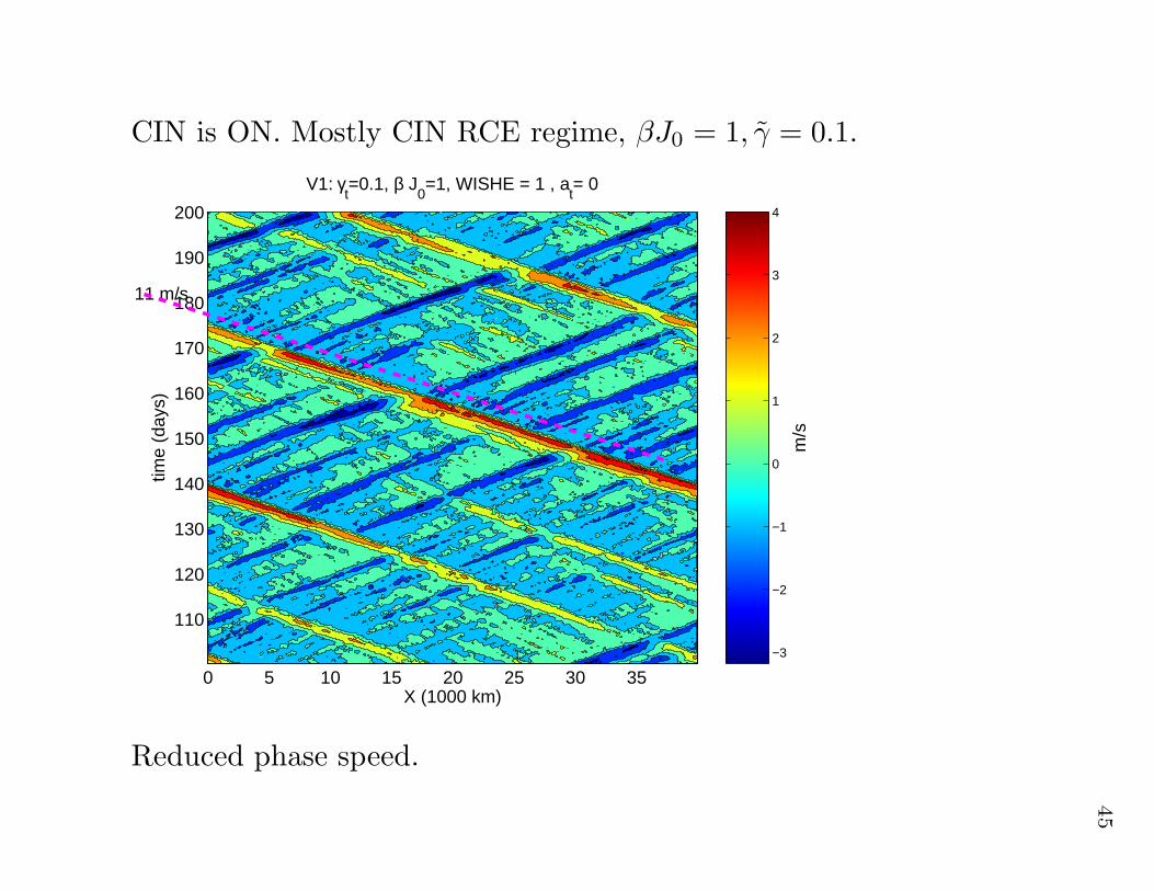
CIN is ON. Mostly CIN RCE regime, βJ0 = 1, γ = 0.1.

0 5 10 15 20 25 30 35

110

120

130

140

150

160

170

180

190

200

11 m/s

X (1000 km)

time

(day

s)V1: γ

t=0.1, β J

0=1, WISHE = 1 , a

t= 0

m/s

−3

−2

−1

0

1

2

3

4

Reduced phase speed.

46

WISHE OFF, Mostly CIN RCE regime, βJ0 = 1, γ = 0.1.

10 15 20 25270

275

280

285

290

295

300

X (1000 km)

time

(day

s)

V1: γt=.1, β J

0=1, WISHE = OFF , a

t= 0

8 m/s

−1

−0.8

−0.6

−0.4

−0.2

0

0.2

0.4

0.6

0.8

1

Intermittent bursts of convection. Phase reduced even more 8 m/s.

47

Multiple RCE, βJ0 = 5, γ = 1

0 5 10 15 20 25 30 35

110

120

130

140

150

160

170

180

190

200

X (1000 km)

time

(day

s)

V1: γt=1, β J

0=5, WISHE = 1 , a

t= 0

m/s

Curiously this line is 7.7 m/s

−10

−5

0

5

10

15

0 5 10 15 20 25 30 35

110

120

130

140

150

160

170

180

190

200

X (1000 km)tim

e (d

ays)

CIN: γt=1, β J

0=5, WISHE = 1 , a

t= 0

0.1

0.2

0.3

0.4

0.5

0.6

0.7

0.8

0.9

Highly intermittent strong bursts.

Is this the MJO?

48

RMS Time series

0 50 100 150 200 250 3000

0.5

1

1.5

V (

m/s

)

Stochastic 2D: ICAPE atilde


I(bar)=0.51365; µ

0=1

WISHE ON

WISHE OFF

0 50 100 150 200 250 30039

40

41

42

θ (K

)

0 50 100 150 200 250 30066

68

70

72

θ eb (

K)

0 50 100 150 200 250 30048

49

50

θ em

0 50 100 150 200 250 3000.4

0.6

0.8

CIN

: ΣI

time (days)

0 50 100 150 200 250 3000

0.5

1

1.5

V (

m/s

)

Stochastic 2D: ICAPE atilde


I(bar)=0.51365; µ

0=1

STOCH CIN OFF

0 50 100 150 200 250 30039

40

41

42

θ (K

)

0 50 100 150 200 250 30066

68

70

72

θ eb (

K)

0 50 100 150 200 250 30048

49

50

θ em

0 50 100 150 200 250 3000.4

0.6

0.8

CIN

: ΣI

time (days)

49

Concluding Remarks

• Coarse graining of systematic microscopic lattice model

• Birth-death process for CIN within a coarse (GCM) grid cell

• Toy GCM: Effects both tropical waves and climate

• Mean field RCEs: PAC, CIN, multiple equilibria, different

stability features and Stochastic dynamics, 3 regimes

• Multiple RCEs, statistically CIN state, intrmittent long

excurtions to PAC RCE

• CIN (dominated, single) RCE regimes: Highly intermittent

with strong oscillations

• Bursts of strong convective events in an environment which is

otherwise dominated by CIN

• Effect on WISHE waves: intermittency, reduced phase speed,

increased wave amplitude.

50

Stochastic multicloud model

• based on multivariable markov chain

• three cloud types, interacting with each other and with large

scale/resolved variables.

• will be presented at next-week’s workshop.

coarse grained stochastic birth-death processes for ... · coarse grained stochastic birth-death...

Documents