clustering：k-means, expect-maximization and gaussian mixture model

XJinliaXXngXXXXXXXX

[email protected] of Computer Science

Institute of Network Technology . BUPT

May 20, 2016

K-means, E.M. and Miture ModelsK-means, E.M. and Mixture Models

Remind:Two ``-MainProblemsinML

• Two- mainproblemsinML:

– Regression: Linear Regression, Neural net...– Classification: Decision Tree, kNN, Bayessian Classifier...

• Today, we will learn:

– K-means: a trivial unsupervised classification algorithm.– Expectation Maximization: a general algorithm for density estimation.

∗ We will see how to use EM in general cases and in specific case of GMM.– GMM: a tool for modelling Data-in-the-Wild (density estimator)

∗ We also learn how to use GMM in a Bayessian Classifier

Contents

• Unsupervised Learning

• K-means clustering

• Expectation Maximization (E.M.)

• Gaussian mixtures as a Density Estimator

– Gaussian mixtures– EM for mixtures

• Gaussian mixtures for classification

Unsupervised Learning

•– Label of each sample is included in the training set

Sample Labelx1 y1... ...xn yk

• Unsupervised learning:– Traning set contains the samples only

Sample Labelx1...xn

Supervised learning techniques:

Unsupervised Learning

−10 0 10 20 30 40 500

10

20

30

40

50

60

(a) Supervised learning.

−10 0 10 20 30 40 500

10

20

30

40

50

60

(b) Unsupervised learning.

Figure 1: Unsupervised vs. Supervised Learning

What is unsupervised learning useful for?

• Collecting and labeling a large training set can be very expensive.

• Be able to find features which are helpful for categorization.

• Gain insight into the natural structure of the data.

Contents







K-means clustering• Clustering algorithms aim to find

groups of “similar” data points amongthe input data.

• K-means is an effective algorithm to ex-tract a given number of clusters from atraining set.

• Once done, the cluster locations canbe used to classify data into distinctclasses. −10 0 10 20 30 40 50

0

10

20

30

40

50

60

K-means clustering

• Given:

– The dataset: {xn}Nn=1 = {x1, x2, ..., xN}

– Number of clusters: K (K < N)

• Goal: find a partition S = {Sk}Kk=1 so that it minimizes the objective function

J =N∑

n=1

K∑k=1

rnk ∥ xn − µk ∥2 (1)

where rnk = 1 if xn is assigned to cluster Sk, and rnj = 0 for j ̸= k.

i.e. Find values for the {rnk} and the {µk} to minimize (1).

K-means clustering

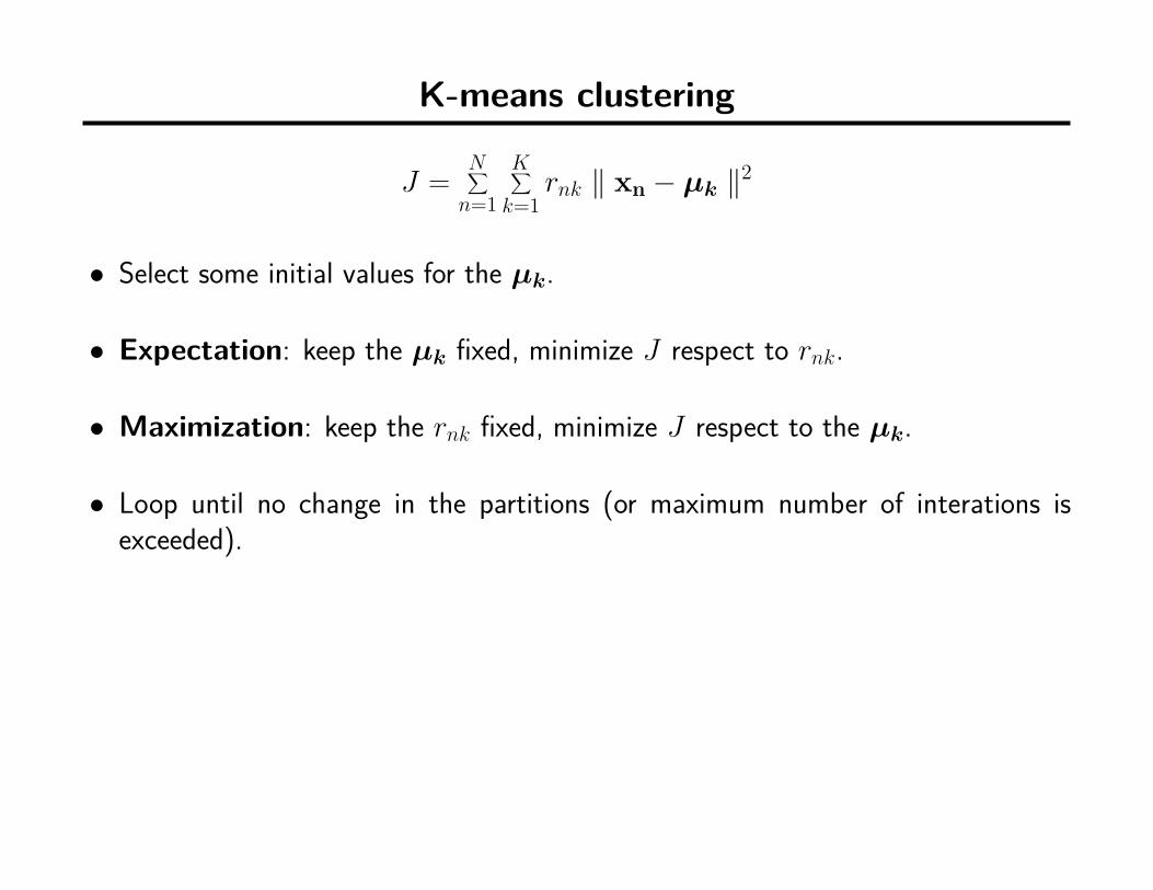
J =N∑

n=1

K∑k=1

rnk ∥ xn − µk ∥2

• Select some initial values for the µk.

• Expectation: keep the µk fixed, minimize J respect to rnk.

• Maximization: keep the rnk fixed, minimize J respect to the µk.

• Loop until no change in the partitions (or maximum number of interations isexceeded).

K-means clustering

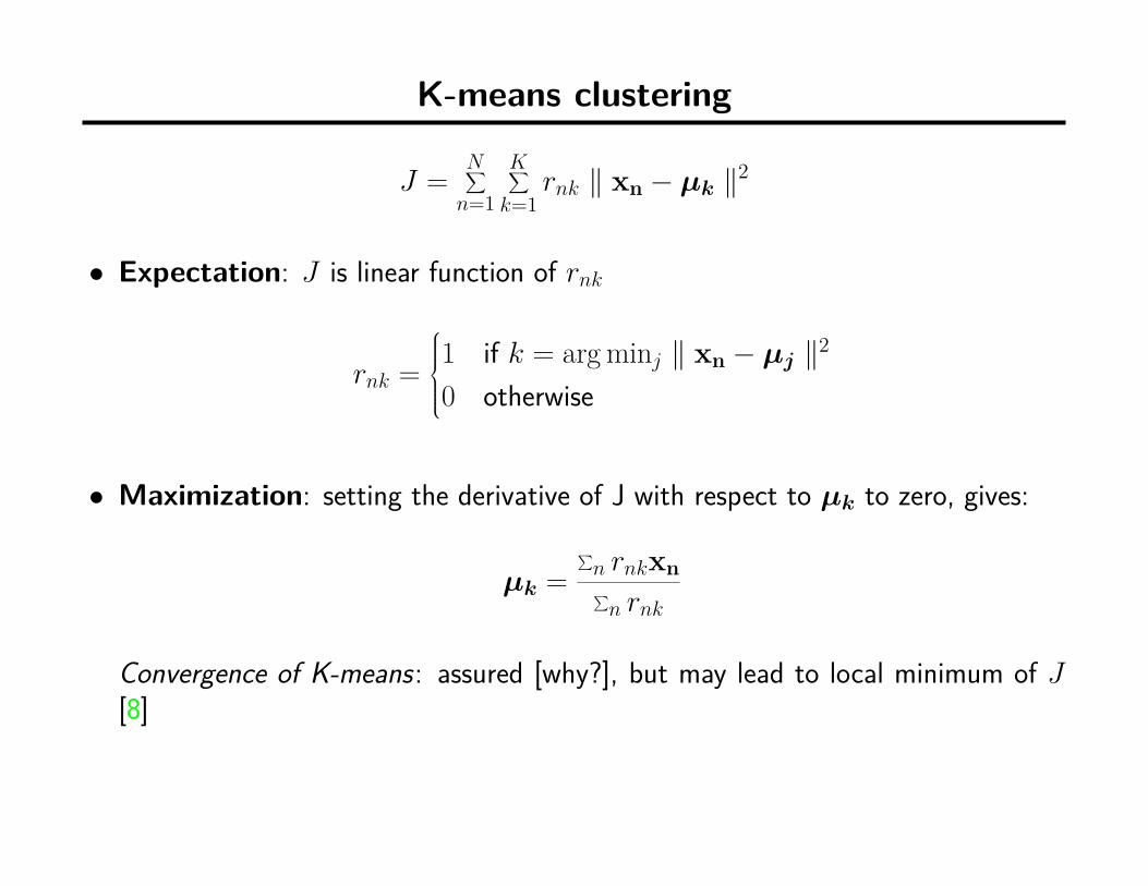
J =N∑

n=1

K∑k=1


• Expectation: J is linear function of rnk

rnk =1 if k = arg minj ∥ xn − µj ∥2

0 otherwise

• Maximization: setting the derivative of J with respect to µk to zero, gives:

µk =∑

n rnkxn∑n rnk

Convergence of K-means: assured [why?], but may lead to local minimum of J[8]

K-means clustering: How to understand?

J =N∑

n=1

K∑k=1


• Expectation: minimize J respect to rnk

– For each xn, find the “closest” cluster mean µk and put xn into cluster Sk.

• Maximization: minimize J respect to µk

– For each cluster Sk, re-estimate the cluster mean µk to be the average valueof all samples in Sk.

• Loop until no change in the partitions (or maximum number of interations isexceeded).

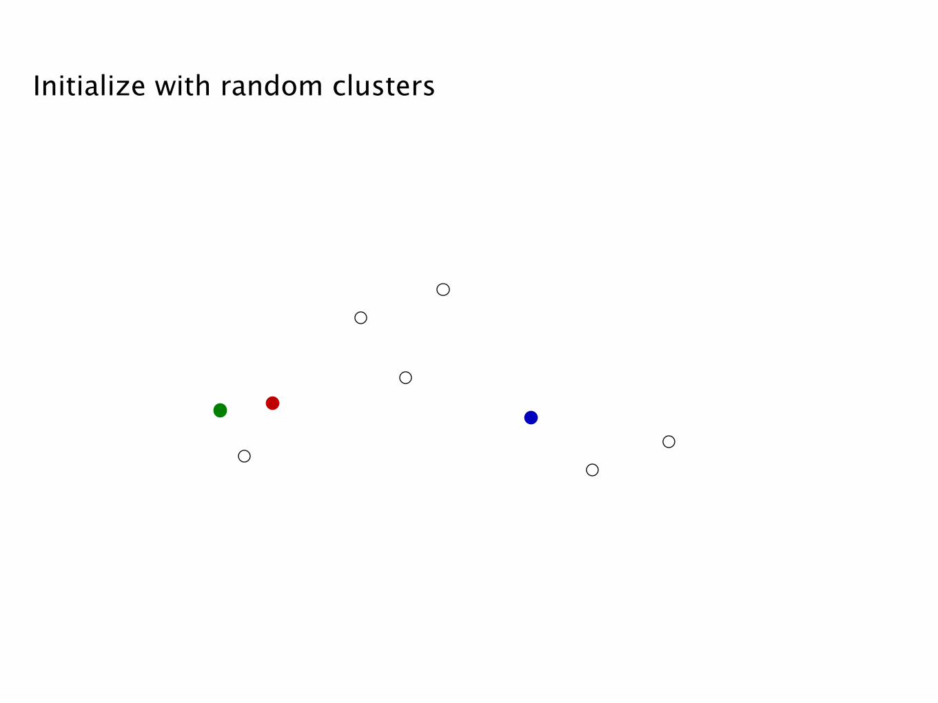
Initialize with random clusters

Assign each point to nearest center

Recompute optimum centers (means)

Repeat: Assign points to nearest center

Repeat: Recompute centers

Repeat...

Repeat...Until clustering does not change

Repeat...Until clustering does not change

Total error reduced at every step - guaranteed to converge.

K-means clustering: some variations

• Initial cluster centroids:

– Randomly selected– Iterative procedure: k-mean++ [2]

• Number of clusters K:

– Empirically/experimentally: 2 ∼√

n– Learning [6]

• Objective function:

– General dissimilarity measure: k-medoids algorithm.

• Speeding up:

– kd-trees for pre-processing [7]– Triangle inequality for distance calculation [4]

Contents







Expectation Maximization

E.M.

Expectation Maximization

• A general-purpose algorithm for MLE in a wide range of situations.

• First formally stated by Dempster, Laird and Rubin in 1977 [1]

• An excellent way of doing our unsupervised learning problem, as we will see– EM is also used widely in other domains.

EM: a solution for MLE

• Given a statistical model with:

– a set X of observed data,– a set Z of unobserved latent data,– a vector of unknown parameters θ,– a likelihood function L (θ; X, Z) = p (X, Z | θ)

• Roughly speaking, the aim of MLE is to determine θ̂ = arg maxθ L (θ; X, Z)

– We known the old trick: partial derivatives of the log likelihood...– But it is not always tractable [e.g.]– Other solutions are available.

EM: General Case

L (θ; X, Z) = p (X, Z | θ)

• EM is just an iterative procedure for finding the MLE

• Expectation step: keep the current estimate θ(t) fixed, calculate the expectedvalue of the log likelihood function

Q(θ | θ(t)

)= E [log L (θ; X, Z)] = E [log p (X, Z | θ)]

• Maximization step: Find the parameter that maximizes this quantity

θ(t+1) = arg maxθ

Q(θ | θ(t)

)

EM: Motivation

• If we know the value of the parameters θ, we can find the value of latent variablesZ by maximizing the log likelihood over all possible values of Z

– Searching on the value space of Z.

• If we know Z, we can find an estimate of θ

– Typically by grouping the observed data points according to the value of asso-ciated latent variable,

– then averaging the values (or some functions of the values) of the points ineach group.

To understand this motivation, let’s take K-means as a trivial example...

EM: informal description

Both θ and Z are unknown, EM is an iterative algorithm:

1. Initialize the parameters θ to some random values.

2. Compute the best values of Z given these parameter values.

3. Use the just-computed values of Z to find better estimates for θ.

4. Iterate until convergence.

EM Convergence

• E.M. Convergence: Yes

– After each iteration, p (X, Z | θ) must increase or remain [NOT OBVIOUS]– But it can not exceed 1 [OBVIOUS]– Hence it must converge [OBVIOUS]

• Bad news: E.M. converges to local optimum.

– Whether the algorithm converges to the global optimum depends on the ini-tialization.

• Let’s take K-means as an example, again...

• Details can be found in [9].

Contents





– Gaussian mixtures

– EM for mixtures


–

Remind: Bayes Classifier

0 10 20 30 40 50 60 70 80−10

0

10

20

30

40

50

60

70

p (y = i | x) = p (x | y = i) p (y = i)p (x)

Remind: Bayes Classifier

0 10 20 30 40 50 60 70 80−10

0

10

20

30

40

50

60

70

In case of Gaussian Bayes Classifier:

p (y = i | x) =1

(2π)d/2∥Σi∥1/2 exp[−1

2 (x − µi)T Σi (x − µi)]pi

p (x)

How can we deal with the denominator p (x)?

Remind: The Single Gaussian Distribution

• Multivariate Gaussian

N (x; µ, Σ) = 1(2π)d/2 ∥ Σ ∥1/2

exp−1

2(x − µ)T Σ−1 (x − µ)

• For maximum likelihood

0 = ∂ ln N (x1, x2, ..., xN; µ, Σ)∂µ

• and the solution isµML = 1

N

N∑i=1

xi

ΣML = 1N

N∑i=1

(xi − µML)T (xi − µML)

The GMM assumption

• There are k components: {ci}ki=1

• Component ci has an associated meanvector µi

•

•

µ1

µ2

µ3

The GMM assumption



• Each component generates data from aGaussian with mean µi and covariancematrix Σi

• Each sample is generated according tothe following guidelines:

µ1

µ2

µ3

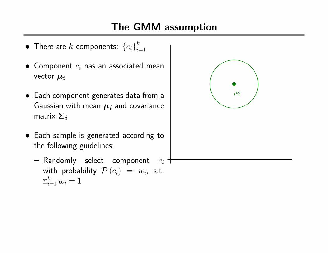
The GMM assumption




• Each sample is generated according tothe following guidelines:– Randomly select component ci

with probability P (ci) = wi, s.t.∑ki=1 wi = 1

µ2

The GMM assumption




• Each sample is generated according tothe following guidelines:

– Randomly select component ci withprobability P (ci) = wi, s.t.∑k

i=1 wi = 1– Sample ~ N (µi, Σi)

µ2

x

Probability density function of GMM

“Linear combination” of Gaussians:

f (x) =k∑

i=1wiN (x; µi, Σi) , where

k∑i=1

wi = 1

0 50 100 150 200 2500

0.002

0.004

0.006

0.008

0.01

0.012

0.014

0.016

0.018

w1N(

µ1, σ2

1

)

w2N(

µ2, σ2

2

)

w3N(

µ3, σ2

3

)

f (x)

(a) The pdf of an 1D GMM with 3 components. (b) The pdf of an 2D GMM with 3 components.

Figure 2: Probability density function of some GMMs.

GMM: Problem definition

f (x) =k∑


k∑i=1

wi = 1

Given a training set, how to model these data point using GMM?

• Given:

– The trainning set: {xi}Ni=1

– Number of clusters: k

• Goal: model this data using a mixture of Gaussians

– Weights: w1, w2, ..., wk

– Means and covariances: µ1, µ2, ..., µk; Σ1, Σ2, ..., Σk

Computing likelihoods in unsupervised case

f (x) =k∑


k∑i=1

wi = 1

• Given a mixture of Gaussians, denoted by G. For any x, we can define thelikelihood:

P (x | G) = P (x | w1, µ1, Σ1, ..., wk, µk, Σk)=

k∑i=1

P (x | ci) P (ci)

=k∑

i=1wiN (x; µi, Σi)

• So we can define likelihood for the whole training set [Why?]

P (x1, x2, ..., xN | G) =N∏

i=1P (xi | G)

=N∏

i=1

k∑j=1

wjN (xi; µj, Σj)

Estimating GMM parameters

• We known this: Maximum Likelihood Estimation

ln P (X | G) =N∑

i=1ln

k∑j=1

wjN (xi; µj, Σj)

– For the max likelihood:0 = ∂ ln P (X | G)

∂µj

– This leads to non-linear non-analytically-solvable equations!

• Use gradient descent

– Slow but doable

• A much cuter and recently popular method...

E.M. for GMM

• Remember:

– We have the training set {xi}Ni=1, the number of components k.

– Assume we know p (c1) = w1, p (c2) = w2, ..., p (ck) = wk

– We don’t know µ1, µ2, ..., µk

The likelihood:

p (data | µ1, µ2, ..., µk) = p (x1, x2, ..., xN | µ1, µ2, ..., µk)=

N∏i=1

p (xi | µ1, µ2, ..., µk)

=N∏

i=1

k∑j=1

p (xi | wj, µ1, µ2, ..., µk) p (cj)

=N∏

i=1

k∑j=1

K exp− 1

2σ2

(xi − µj

)2wi

E.M. for GMM

• For Max. Likelihood, we know ∂∂µi

log p (data | µ1, µ2, ..., µk) = 0• Some wild algebra turns this into: For Maximum Likelihood, for each j:

µj =

N∑i=1

p (cj | xi, µ1, µ2, ..., µk) xi

N∑i=1

p (cj | xi, µ1, µ2, ..., µk)

This is N non-linear equations of µj’s.• So:

– If, for each xi, we know p (cj | xi, µ1, µ2, ..., µk), then we could easily computeµj,

– If we know each µj, we could compute p (cj | xi, µ1, µ2, ..., µk) for each xi

and cj.

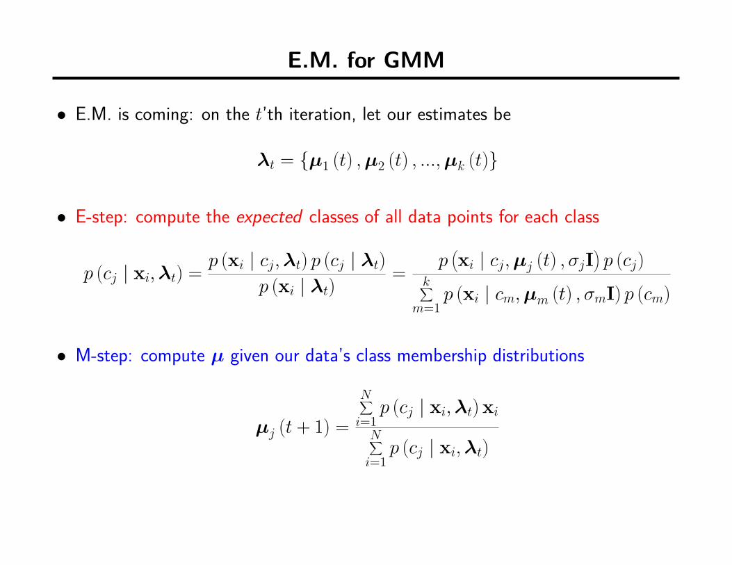
E.M. for GMM

• E.M. is coming: on the t’th iteration, let our estimates be

λt = {µ1 (t) , µ2 (t) , ..., µk (t)}

• E-step: compute the expected classes of all data points for each class

p (cj | xi, λt) = p (xi | cj, λt) p (cj | λt)p (xi | λt)

= p(xi | cj, µj (t) , σjI

)p (cj)

k∑m=1

p (xi | cm, µm (t) , σmI) p (cm)

• M-step: compute µ given our data’s class membership distributions

µj (t + 1) =

N∑i=1

p (cj | xi, λt) xi

N∑i=1

p (cj | xi, λt)

E.M. for General GMM: E-step

• On the t’th iteration, let our estimates be

λt = {µ1 (t) , µ2 (t) , ..., µk (t) , Σ1 (t) , Σ2 (t) , ..., Σk (t) , w1 (t) , w2 (t) , ..., wk (t)}

• E-step: compute the expected classes of all data points for each class

τij (t) ≡ p (cj | xi, λt) = p (xi | cj, λt) p (cj | λt)p (xi | λt)

= p(xi | cj, µj (t) , Σj (t)

)wj (t)

k∑m=1

p (xi | cm, µm (t) , Σj (t)) wm (t)

E.M. for General GMM: M-step

• M-step: compute µ given our data’s class membership distributions

wj (t + 1) =

N∑i=1

p (cj | xi, λt)

Nµj (t + 1) =

N∑i=1

p (cj | xi, λt) xi

N∑i=1

p (cj | xi, λt)

= 1N

N∑i=1

τij (t) = 1Nwj (t + 1)

N∑i=1

τij (t) xi

Σj (t + 1) =

N∑i=1

p (cj | xi, λt)[xi − µj (t + 1)

] [xi − µj (t + 1)

]TN∑

i=1p (cj | xi, λt)

= 1Nwj (t + 1)

N∑i=1

τij (t)[xi − µj (t + 1)

] [xi − µj (t + 1)

]T

E.M. for General GMM: Initialization

• wj = 1/k, j = 1, 2, ..., k

• Each µj is set to a randomly selected point

– Or use K-means for this initialization.

• Each Σj is computed using the equation in previous slide...

Gaussian Mixture Example: Start

After first iteration

After 2nd iteration

After 3rd iteration

After 4th iteration

After 5th iteration

After 6th iteration

After 20th iteration

Local optimum solution

• E.M. is guaranteed to find the local optimal solution by monotonically increasingthe log-likelihood

• Whether it converges to the global optimal solution depends on the initialization

−10 −5 0 5 10 150

2

4

6

8

10

12

14

16

18

−10 −5 0 5 10 150

5

10

15

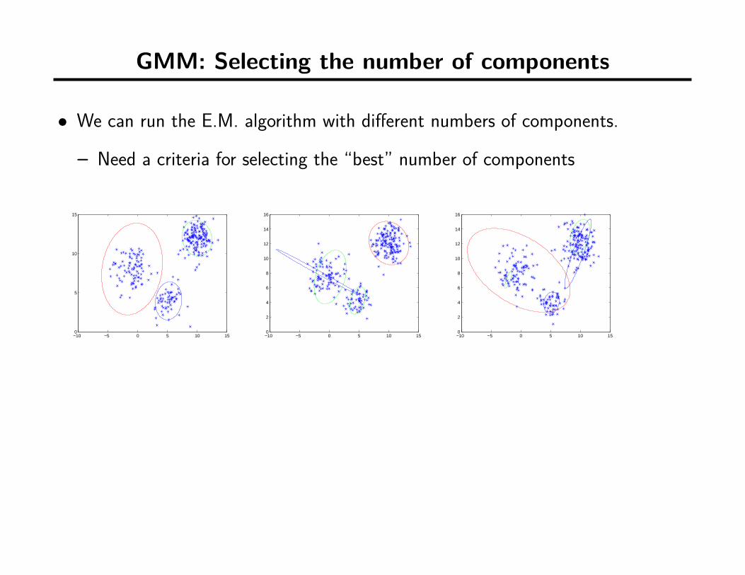
GMM: Selecting the number of components

• We can run the E.M. algorithm with different numbers of components.

– Need a criteria for selecting the “best” number of components

−10 −5 0 5 10 150

5

10

15

−10 −5 0 5 10 150

2

4

6

8

10

12

14

16

−10 −5 0 5 10 150

2

4

6

8

10

12

14

16

Contents




– Regularized EM– Model Selection




Gaussian mixtures for classification

p (y = i | x) = p (x | y = i) p (y = i)p (x)

• To build a Bayesian classifier based on GMM, we can use GMM to model data ineach class

– So each class is modeled by one k-component GMM.

• For example:Class 0: p (y = 0) , p (x | θ0), (a 3-component mixture)Class 1: p (y = 1) , p (x | θ1), (a 3-component mixture)Class 2: p (y = 2) , p (x | θ2), (a 3-component mixture)...

GMM for Classification

• As previous, each class is modeled by a k-component GMM.

• A new test sample x is classified according to

c = arg maxi

p (y = i) p (x | θi)

wherep (x | θi) =

k∑i=1

wiN (x; µi, Σi)

• Simple, quick (and is actually used!)

References

[1] N. Laird A. Dempster and D. Rubin. Maximum likelihood from incomplete datavia the em algorithm. Journal of the Royal Statistical Society. Series B (Method-ological), 39(1):pp. 1–38., 1977.

[2] David Arthur and Sergei Vassilvitskii. k-means ++ : The Advantages of CarefulSeeding. In Proceedings of the eighteenth annual ACM-SIAM symposium onDiscrete algorithms, volume 8, pages 1027–1035, 2007.

[3] N. Gumerov C. Yang, R. Duraiswami and L. Davis. Improved fast gauss transformand efficient kernel density estimation. In IEEE International Conference onComputer Vision, pages pages 464–471, 2003.

[4] Charles Elkan. Using the Triangle Inequality to Accelerate k-Means. In Proceed-

ings of the Twentieth International Conference on Machine Learning (ICML),2003.

[5] Keshu Zhang Haifeng Li and Tao Jiang. The regularized em algorithm. InProceedings of the 20th National Conference on Artificial Intelligence, pagespages 807 – 812, Pittsburgh, PA, 2005.

[6] Greg Hamerly and Charles Elkan. Learning the k in k-means. In In NeuralInformation Processing Systems. MIT Press, 2003.

[7] Tapas Kanungo, David M Mount, Nathan S Netanyahu, Christine D Piatko, RuthSilverman, and Angela Y Wu. An efficient k-means clustering algorithm: anal-ysis and implementation. IEEE Transactions on Pattern Analysis and MachineIntelligence, 24(7):881–892, July 2002.

[8] J MacQueen. Some methods for classification and analysis of multivariate obser-vations. In Proceedings of 5th Berkeley Symposium on Mathematical Statisticsand Probability, volume 233, pages 281–297. University of California Press, 1967.

[9] C.F. Wu. On the convergence properties of the em algorithm. The Annals ofStatistics, 11:95–103, 1983.

clustering：k-means, expect-maximization and gaussian mixture model

Data & Analytics