Cluster analysis methodsfor speech recognition

Julien Neel (ENST Paris)

Centre forSpeech Technology

Supervisor: Giampiero Salvi

Approved: 2005-02-18

Examiner: Rolf Carlson

. . . . . . . . . . . . . . . . . . . . . . .

(signature)

Stockholm Examenarbete i Talteknologi17th February 2005 (Master Thesis in Speech Technology)

Department of Speech, Music and HearingRoyal Institute of TechnologyS-100 44 Stockholm

Examensarbete i Talteknologi

Klustringmetoder for taligenkanning

Julien Neel (ENST Paris)

Godkant:2005-02-18

Examinator:Rolf Carlson

Handledare:Giampiero Salvi

Abstract

How well can clustering methods capture a phonetic classification? Can the ”appropriate”number of clusters be determined automatically? Which kinds of phonetical featuresgroup together naturally? How can clustering quality be measured?” To what extent isan automatic clustering method reliable in this case?

This study tries to answer these questions with a number of experiments conducted onspeech data using K-means and fuzzy K-means clustering. Optimal number of clusterswere determined with the Davies Bouldin and I family indexes.

For this report, the data considered was extracted from the TIMIT database, a corpusof read speech with phoneme transcription. A small clustering toolbox for Matlab wasimplemented. It computed clusterings using various classical methods and cluster validityindexes to assess quality. A number of benchmark tests were run on the IRIS data as wellas synthetic data.

The speech examples, show that when clustering phonemes, certain acoustical andarticulatory features can be captured. Fuzzy clustering can improve cluster quality. Theindexes, which yield an optimal number of clusters according to a criterion to optimize, donot give us the number of phonemes, but can help spot broad phonetic classes. Anotherphonetic classification, based on both acoustic and articulatory features is more naturalthan broad phonetic classes.

Clustering methods can also help ranking the importance of acoustical/articulatoryfeatures such as those of Jackobson, Halle and Fant. Some of these features emergenaturally from the observations.

Acknowledgments

I would like to thank Bjorn Granstrom and Rolf Carlson for their warm welcome andfor giving me the opportunity to do my internship as a master thesis student in theSpeech Department of KTH, Giampiero Salvi for tutoring me in discovering research, myfellow colleagues Linda Oppelstrup for the late nights, Elina Eriksson and Sara Ohgren forenlightening days, and Anders Lundgren for his curiosity, Gunilla Svanfeldt and PrebenWik for the advice and chats, Niclas Horney for having fixed my computer and unlockedmy account every two weeks, and Catrin Dunger for having been so helpful. Thanks toall the members of the Speech Department for the great working atmosphere and thewonderful Christmas party.

LIST OF FIGURES LIST OF FIGURES

List of Figures

1 Speech spectral characteristics . . . . . . . . . . . . . . . . . . . . . . . . . . 32 Illustration of the short-time energy and ZCR coefficients . . . . . . . . . . 43 A sample spectrum from the TIMIT speech data base . . . . . . . . . . . . . 54 Illustration of the K-means algorithm . . . . . . . . . . . . . . . . . . . . . 95 Synthetic data sets: 5 well-separated clusters, 5 overlapping, 2 rings . . . . 156 Fisher’s Iris data set . . . . . . . . . . . . . . . . . . . . . . . . . . . . . . . 167 Synthetic fuzzy data set and clustering results . . . . . . . . . . . . . . . . . 178 Feature data extraction and clustering procedure . . . . . . . . . . . . . . . 199 {d,t,s,z,iy,eh,ao}: data in 2D-PCA projection . . . . . . . . . . . . . . 2010 {d,t,s,z,iy,eh,ao}: cumulated scatter on principal factors (left), corre-

lation between factors and feature dimensions (right) . . . . . . . . . . . . . 2111 {d,t,s,z,iy,eh,ao}: I (left) and DB (right) index crisp clustering . . . . 2212 {s,f,v,iy}: data in 2D-PCA projection (left) and indices (right) . . . . . . 2313 {s,f,v,iy}: DB clustering results . . . . . . . . . . . . . . . . . . . . . . . 2414 {ae,ah,aa}: feature data in 2D-PCA . . . . . . . . . . . . . . . . . . . . . 2515 {ae,ah,aa}: content of the clusters . . . . . . . . . . . . . . . . . . . . . . . 2516 {ae,ah,aa}: principal comp. correlation with feature dimensions . . . . . . 2617 {s,z,v,f}: feature data in 2D-PCA . . . . . . . . . . . . . . . . . . . . . . 2618 {s,z,v,f}: principal comp. correlation with feature dimensions . . . . . . . 2719 {s,z,v,f}: crisp (top) and fuzzy (bottom) clustering results . . . . . . . . 2820 {s,z,v,f}: speech spectrum for si2036 . . . . . . . . . . . . . . . . . . . . 2821 {s,z,v,f}: cluster assignments in time for si2036 . . . . . . . . . . . . . . 28

ii

LIST OF TABLES LIST OF TABLES

List of Tables

1 Broad phonetic classes in speech . . . . . . . . . . . . . . . . . . . . . . . . 22 Illustration of 4 of the 14 binary features from Jackobson’s classification . . 63 Sample data sets: recommended number of clusters . . . . . . . . . . . . . . 164 {d,t,s,z,iy,eh,ao}: TIMIT lexicon of phonemic and phonetic symbols . . 205 {ae,ah,aa}: TIMIT lexicon of phonemic and phonetic symbols . . . . . . . 246 {ae,ah,aa}: formant frequencies of vowels . . . . . . . . . . . . . . . . . . . 247 {s,z,v,f}: Best K for each index and measure . . . . . . . . . . . . . . . . 278 {s,z,v,f}: Binary feature classification . . . . . . . . . . . . . . . . . . . . 29

iii

LIST OF TABLES LIST OF TABLES

List of Abbreviations

ASR Automatic speech recognitionDB Davies Bouldin indexEM Expectation maximization algorithmFmeas F-measure indexGMM Gaussian mixture modelsMACF Maximum of the autocorrelation functionMFCC Mel frequency cepstrum coefficientsPCA Principal component analysisSVC Support vector clusteringZCR Average zero-crossing rate

iv

CONTENTS CONTENTS

Contents

1 Introduction 1

1.1 Method and problem formulation . . . . . . . . . . . . . . . . . . . . . . . . 11.2 Outline of the report . . . . . . . . . . . . . . . . . . . . . . . . . . . . . . . 1

2 Theory 2

2.1 Phonetic feature model . . . . . . . . . . . . . . . . . . . . . . . . . . . . . . 22.1.1 Phonemes . . . . . . . . . . . . . . . . . . . . . . . . . . . . . . . . . 22.1.2 Feature vectors for speech . . . . . . . . . . . . . . . . . . . . . . . . 22.1.3 Problems linked to phonetic representation . . . . . . . . . . . . . . 52.1.4 Phoneme classifications . . . . . . . . . . . . . . . . . . . . . . . . . 6

2.2 Clustering basics . . . . . . . . . . . . . . . . . . . . . . . . . . . . . . . . . 62.2.1 Introduction . . . . . . . . . . . . . . . . . . . . . . . . . . . . . . . 62.2.2 Applications . . . . . . . . . . . . . . . . . . . . . . . . . . . . . . . 72.2.3 Problems . . . . . . . . . . . . . . . . . . . . . . . . . . . . . . . . . 72.2.4 Clustering algorithms overview . . . . . . . . . . . . . . . . . . . . . 8

2.3 Clustering algorithms used . . . . . . . . . . . . . . . . . . . . . . . . . . . . 82.3.1 K-means . . . . . . . . . . . . . . . . . . . . . . . . . . . . . . . . . . 82.3.2 Fuzzy K-means . . . . . . . . . . . . . . . . . . . . . . . . . . . . . . 92.3.3 Gaussian Mixture Models and EM algorithm . . . . . . . . . . . . . 10

2.4 Cluster indexes and validity measures . . . . . . . . . . . . . . . . . . . . . 112.4.1 Davies-Bouldin index . . . . . . . . . . . . . . . . . . . . . . . . . . 112.4.2 The I indexes . . . . . . . . . . . . . . . . . . . . . . . . . . . . . . . 122.4.3 F-measure . . . . . . . . . . . . . . . . . . . . . . . . . . . . . . . . . 122.4.4 Purity . . . . . . . . . . . . . . . . . . . . . . . . . . . . . . . . . . . 132.4.5 Principal component analysis . . . . . . . . . . . . . . . . . . . . . . 13

3 Method and implementation 15

3.1 Creating benchmarks . . . . . . . . . . . . . . . . . . . . . . . . . . . . . . . 153.1.1 Data sets . . . . . . . . . . . . . . . . . . . . . . . . . . . . . . . . . 153.1.2 Tested clustering methods . . . . . . . . . . . . . . . . . . . . . . . . 153.1.3 Results . . . . . . . . . . . . . . . . . . . . . . . . . . . . . . . . . . 15

3.2 Working with TIMIT speech data . . . . . . . . . . . . . . . . . . . . . . . . 173.2.1 The TIMIT speech corpus . . . . . . . . . . . . . . . . . . . . . . . . 173.2.2 Extracted features . . . . . . . . . . . . . . . . . . . . . . . . . . . . 173.2.3 Implementation . . . . . . . . . . . . . . . . . . . . . . . . . . . . . . 183.2.4 How many clusters? . . . . . . . . . . . . . . . . . . . . . . . . . . . 18

4 Results 20

4.1 Example 1: broad phonetic classes {d,t,s,z,iy,eh,ao} . . . . . . . . . . . 204.2 Example 2: vowels/consonants {s,f,v,iy} . . . . . . . . . . . . . . . . . . 234.3 Example 3: front/open vowels {ae,ah,aa} . . . . . . . . . . . . . . . . . . . 244.4 Example 4: fricatives {s,z,v,f} . . . . . . . . . . . . . . . . . . . . . . . . 26

5 Discussion 30

6 Conclusion and further work 31

v

1 INTRODUCTION

1 Introduction

1.1 Method and problem formulation

Clustering methods have traditionally been used in order to find emerging patterns fromdata sets with unknown properties. Clustering is a ill-defined problem for which thereexist numerous methods (see [4, 10, 16, 1]). Unfortunately, many articles that dealt withclustering did not take into account high dimensional data sets, as it is the case in speech.

In this study a number of clustering algorithms, including K-means and fuzzy K-means, have been tested both on benchmark data (IRIS and various synthetic data cloudswith ellipsoidal or chainlike shapes, such as rings) and on the TIMIT speech database, withrecordings of American English speakers. Benchmark data has been also tested with aSupport Vector Clustering procedure, but for reasons of computational time on simpledata sets, this method was not retained for speech data.

The Matlab routines extracted feature vectors from the feature files, classified themusing the TIMIT transcription file, stored the results and displayed various visualizationsfor interpretation. Various data sets for training and testing were prepared. The focusof the experiments was initially to estimate the performance of clustering methods in aclassification task where each cluster was assigned the phonetic class closest to it.

Other experiments were conducted in order to investigate upon the information suchclustering procedures could find. Clustering results were analyzed visually in 2D, as his-tograms resuming how clusters captured the classes, and with Wavesurfer, in order todisplay cluster assignments in time. Since the data contained overlapping clusters andoutliers and had many dimensions, it was difficult to estimate visually in two dimensionshow well natural groups appeared.

Therefore, additional indexes and validity indexes to assess cluster quality were com-puted: the F -measure, purity and the partition coefficient PC. These provide severalmeasures of the quality of the clustering with respect to the classification.

1.2 Outline of the report

The report is organized as follows: Section 2 presents basics on phonetic feature modelsand on the clustering procedures used. Cluster validity is also discussed here. Section 3describes the experimental settings and method. Some results are presented in Section 4and discussed in section 5. Finally, section 6 concludes the report.

1

2 THEORY

2 Theory

2.1 Phonetic feature model

2.1.1 Phonemes

In linguistics, the fundamental unit of speech is the phoneme. Phonemes are the basictheoretical units for describing how speech conveys meaning. They compose a family ofsimilar sound groups. Its members, the allophones, are considered equivalent for a givenlanguage.

In English for example, [ph] and [p] are allophones of the phoneme p, as in pit and spit.The first consonant of pit has an extra puff of air after it which is not found after the [p]of spit. However, switching allophones of the same phoneme won’t change the meaning ofthe word: [sphIt] still means spit. Switching allophones of different phonemes will changethe meaning of the word or result in a nonsense word: [skIt] and [stIt] do not mean spit.

Different languages can have different groupings for their phonemes. [p] and [ph] belongto the same phoneme in English, but to different phonemes in Chinese. In Chinese,switching [p] and [ph] does change the meaning of the word.

A broad transcription uses only one symbol for all allophones of the same phoneme.This is enough information to distinguish a word from other words of the language. Whatdetails you have to include in a broad transcription will depend on what language ordialect you are transcribing.

In English, there are about 42 phonemes. They tradionally fall into the followingcategories: vowels (front, mid or back), diphthongs, semi-vowels (glides and liquids) andconsonants (stops, plosives, nasals, fricatives and affricates).

Phonetic classes Sample phonemes

stops b, d, g, p, t, k

affricates ch

fricatives s, sh, z, f

nasals m, n, ng

semivowels & glides l, r, w, y

vowels ah, aa, eh, iy, uw

Table 1: Broad phonetic classes in speech

Each sound has particular spectral characteristics. These characteristics change con-tinuously in time. The patterns of change give cues to phone identity. However, speechspectra (see figure 1) also include numerous sources of variability. Emotion and phoneticcontext for example can change a person’s way of speaking, and it can be a great source ofspeaker intravariability. Spectra vary even more when the same utterance is pronouncedby speakers of different gender, speaking style, etc.

2.1.2 Feature vectors for speech

The underlying assumption of local stationarity in most speech processing methods is thatthe properties of the speech signal change relatively slowly with time. This assumptionleads to a variety of short-time processing methods in which short segments of the speech

2

2 THEORY 2.1 Phonetic feature model

S IH K S TH R IY UW NAHsix three one

Figure 1: Speech spectral characteristics

signal are isolated and processed as if they were short segments from a sustained sound withfixed properties. These short segments called time analysis frames overlap one another.The result of the processing on each frame is a new time-dependant sequence which canserve as a representation of the speech signal.

The feature vectors represent the speech signal. Each dimension requires processingmethods that involve the waveform of speech signal directly and others require using thespectrum of the speech signal. They are called time-domain and frequency-domain meth-ods. Measurements such as energy, zero-crossing rate and the autocorrelation function areof the first type, and mel-cepstrum coefficients are of the second type.

The feature dimensions are described below.

Short-time energy: The amplitude of the speech signal varies appreciably with time.In particular, the amplitude of unvoiced segments is generally much lower than the ampli-tude of voiced segments. The short-time energy of the speech signal provides a convenientrepresentation that reflects these amplitude variations. The energy function can also beused to locate approximately the time at which voiced speech becomes unvoiced, and viceversa, and, for very high quality speech (high signal-to-noise ratio), the energy can be usedto distinguish speech from silence. The formula for short-time energy is:

En =∑

−M≤m≤M

[x(m) ∗ w(n−m)]2 (1)

An illustration of short-time energy can be found in figure 2.

Short-time average zero-crossing rate: In the context of discrete-time signals, azero-crossing is said to occur if successive samples have different algebraic signs. Thismeasure gives a reasonable way to estimate the frequency of a sine wave. Speech signalsare broadband signals and the interpretation of average zero-crossing is therefore muchless precise. Since high frequencies imply high zero-crossing rate and low frequencies implylow zero-crossing rates, there is a strong correlation between zero crossing rate and energydistribution with frequency. A reasonable generalization is that if the zero-crossing rate ishigh, the speech signal is unvoiced, while if the zero-crossing rate is low, the speech signal

3

2.1 Phonetic feature model 2 THEORY

is voiced. This however, is a very imprecise statement because high and low remain tobe defined. Energy and zero-crossing rate can help to discriminate speech from silence,making it possible to process only the parts of the input that correspond to speech. Theformula for short-time average zero-crossing rate is:

Zn =∑

−M≤m≤M

|sgn[x(m)]− sgn[x(m− 1)] | ∗w(n−m) (2)

An illustration of short-time average zero-crossing rate can be found in figure 2.

Figure 2: Illustration of the short-time energy and ZCR coefficients

Short-time autocorrelation function: It is a version of the autocorrelation functionadapted to the short-time representation. It is an even function, attains its maximal valuein 0, and this supremum is equal to the energy for deterministic signals or the average powerfor random or periodic signals. Periodicity in the signal is given by the first maximumin the function. This property makes the autocorrelation function a means for estimatingperiodicity in many signals, including speech. It contains much more information aboutthe detailed structure of the signal. The formula for short-time autocorrelation is:

Rn(k) =

N−1−k∑

m=0

[x(n + m)w′(m)] ∗ [x(n + m + k)w′(m + k)] (3)

Mel-cepstrum coefficients: Front-end analysis aims at extracting phonetically sig-nificant acoustic information for the human ear. This useful information can be capturedusing the short-term spectrum and mathematical approximations concerning its local sta-tionarity. Human ability to perceive a certain frequency f is influenced by the energy ina critical band of frequencies, whose size depends on the considered frequency f . Becausethe filtering operation of the vocal tract is the most influential factor in determining pho-netic properties of speech sounds, it is desirable to separate out the excitation componentg(t) from the filter component h(t) in the signal s(t):

s(t) = g(t) ∗ h(t) (4)

4

2 THEORY 2.1 Phonetic feature model

Cepstral analysis is a technique for estimating a separation of the source and filter com-ponents. The mel-cepstrum, introduced by Davies and Mermelstein, exploits auditoryprinciples, as well as the decorrelating property of the cepstrum. In addition, the mel-cepstrum is amenable to compensation for convolutional channel distortion. As such, theMFCCs have proven to be one of the most successful feature representations in speech-related recognition tasks.

A filter bank, with triangular filters placed according to an empirical log-linear scalecalled the mel-scale, is constructed to resemble the human auditory system with morechannels at low frequencies and fewer at high. This makes it easier to estimate the fre-quencies of the formants and thus the phone being uttered. Filtering the spectrum (alsocalled liftering) can be applied to remove certain components or alter the relative influ-ence of the different components. Most of the influence of the fundamental frequency isactually removed from the spectrum. The resulting spectrum can be much smoother thanthe original and show the formant peaks more clearly (see [12]).

2.1.3 Problems linked to phonetic representation

Although well-defined gaps are often perceived between words in a language we speak,this is often an illusion. Examining the actual the actual physical speech signal, one oftenfinds undiminished sound energy at word boundaries. Indeed, Indeed, a drop in speechenergy is as likely to occur within a word as between words. This property of speechis particularly compelling when we listen to someone speaking a foreign language. Thespeech appears to be a continuous stream of sounds with no obvious word boundaries. Itis our familiarity with our own language that leads to the illusion of word boundaries.

Within a single word, even greater segmentation problems exist. These intra-wordproblems involve the identification of the basic vocabulary of speech sounds: phonemes.A segmentation problem arises when the phonemes composing a spoken word need to beidentified. Segmentation at this level is like recognizing a manually written text whereone letter runs into another. Also, as in the case of writing, different speakers vary in theway they produce the same phonemes. The variation among speakers is strong.

In this report, we will be dealing with general segmenting of speech into words/phonemes.We will consider each frame as a data point, therefore the utterance of a given phonemewill be represented as many times as there are such data points.

Figure 3: A sample spectrum from the TIMIT speech data base

A further difficulty in speech perception involves a phenomenon known as co-articulation.Consider in figure 3) the spectrum of a female speaker in the New England dialect uttering

5

2.2 Clustering basics 2 THEORY

”she had your dark” and let’s focus on the word dark. As the vocal tract is producing onesound, say the stop [d] in the phoneme sequence [d, ah, kcl, k], it is moving towardsthe shape it needs for the vowel [ah]. Then, as it is saying the [ah], it is moving toproduce the voiced stop [k], with the closure interval of the stop kcl in between. Ineffect, the various phenomenons overlap. This means additional difficulties in segmentingphonemes, and it also means that the actual sound produced for one phoneme will bedetermined by the context of the other surrounding phonemes.

2.1.4 Phoneme classifications

Classical Phonetics use the place-manner classification system for consonants and thehigh-low / front-back system for vowels. The main purpose is to enable the phonetician tospecify how particular sounds are produced with respect to their articulation. It becomespossible to use the features or parameters of the classification system to label whole setsof sounds or articulations. Thus we might refer to the set of all plosives or the set ofall voiced plosives (three in English), or the set of all voiced alveolar plosives (one onlyin English) - and so on, cutting horizontally and vertically around the consonant matrix.Similarly, for vowels, the set of all front vowels, or the set of all rounded vowels, and soon.

Distinctive feature theory was first formalized by Jackobson ad Halle in 1941 (see[7]), and remains one of the most significant contributions to phonology. There havebeen numerous refinements to the set since that date. These features are binary, whichmeans that a phoneme either has the feature (e.g.: [+voice]) or doesn’t have the feature([-voice]). A small set of features is able to differentiate between the phonemes of anysingle language. Distinctive features may be defined in terms of articulatory or acousticfeatures: for example, [grave] is an acoustic feature (concentration of low frequencyenergy) and [high] is an articulatory feature related to tongue height, but it can also bereadily defined in acoustic terms. Jackobson’s features are primarily based on acousticdescriptions.

+/− Acoustic (+) Articulatory (+)

grave/acute concentration of energy in lower frequencies peripheral

voiced/voiceless periodic low frequency excitation periodic vibration of vocal chords

continuant/discontinuous no abrupt transition sound/silence no turning on/off of source

strident/mellow higher intensity noise rough-edged

Table 2: Illustration of 4 of the 14 binary features from Jackobson’s classification

2.2 Clustering basics

2.2.1 Introduction

Clustering is the process of grouping together similar objects. The resulting groups arecalled clusters. Clustering algorithms group data points according to various criteria.Unlike most classification methods, clustering handles data that has no labels, or ignores

6

2 THEORY 2.2 Clustering basics

the labels while clustering. The concept mostly utilizes geometric principles, where thesamples are interpreted as points in a d-dimensional Euclidian space, and clustering ismade according to the distances between points: usually, points which are close to eachother will be allocated to the same cluster.

This method is an unsupervised process since there are no predefined classes and noexamples that would indicate grouping properties in the data set. The various clusteringalgorithms are based on some assumptions in order to define a partitioning of a data set.Most methods behave differently depending on the features of the data set and the initialassumptions for defining groups. Therefore, in most applications, the resulting clusteringscheme requires some sort of evaluation regarding its validity. Evaluating and assessingthe results of a clustering algorithm is the main object of cluster validity ([5, 6]).

2.2.2 Applications

Clustering is one of the most useful method in the data mining process for discoveringgroups and identifying interesting distributions and patterns in the underlying data. Thus,the main concern in the clustering process is to reveal the organization of patterns intosensible groups, which allow us to discover similarities and differences, as well as to deriveuseful inferences about them. Clustering makes it possible to look at properties of wholeclusters instead of individual objects - a simplification that might be useful when handlinglarge amounts of data. It has the potential to identify unknown classification schemes thathighlight relations and differences between objects.

2.2.3 Problems

In the literature (see [11, 10, 16, 2, 4]), a wide variety of algorithms have been proposedfor different applications and sizes of data sets, but there seems to be no unifying theory ofclustering. Most clustering benchmarks deal with low dimensional real world or syntheticdata sets, unlike speech data.

A frequent problem many clustering algorithms encounter is the choice of the numberof clusters. Quite different kinds of clusters may emerge when its value is changed. Mostclustering methods require the user to specify a value, though some provide means toestimate the number of clusters inherent within the data. Among those, Support Vec-tor Machines, model-based methods that use the Bayes information criterion for modelselection, or different kinds of indexes, such as Davies-Bouldin’s index.

Many clustering algorithms prefer certain cluster shapes and sizes, and these algorithmswill always assign the data to clusters of such shapes even when there were no such clustersin the data. For example, K-means is only able to form spherical clusters, and if appliedto concentric ring shaped data, locates all the centroids together in the center of the rings

Handling strongly overlapping clusters or noise in the data is often difficult. For in-stance, when clusters are not well separated and compact, the distance between clustersas the average distance between pairs of samples does not work well. Some algorithms getstuck at local minima and the result is largely dependent on initialization, one of the majordrawbacks of the K-means algorithm. Large data sets or vectors with many componentscan be a serious computational burden.

7

2.3 Clustering algorithms used 2 THEORY

2.2.4 Clustering algorithms overview

A multitude of clustering methods are proposed in the literature (see [11, 10, 16, 2, 4]).Clustering algorithms can be classified according to the type of data input to the algorithm,the clustering criterion defining the similarity between data points, and the theory andfundamental concepts on which clustering analysis techniques are based (e.g.: fuzzy theory,statistics, etc.). Thus according to the method adopted to define clusters, the algorithmscan be broadly classified into the following types:

Partitional clustering attempts to directly decompose the data set into a set of disjointclusters. More specifically, they attempt to determine an integer number of partitions thatoptimize a certain criterion function. The criterion function may emphasize the local orglobal structure of the data and its optimization is an iterative procedure.

Hierarchical clustering proceeds successively by either merging smaller clusters intolarger ones, or by splitting larger clusters. The result of the algorithm is a dendrogram(tree) of clusters which shows how the clusters are related. By cutting the dendrogramat a desired level, a clustering of the data items into disjoint groups is obtained. Thesemethods are often not suitable for large data sets because of computational time.

Density-based clustering groups neighboring objects into clusters based on densityconditions. It is model based and parametric. Gaussian Mixture Models (or weighted sumof gaussian distributions) is a typical example.

Grid-based clustering is mainly proposed for spatial data mining. Their main char-acteristic is that they quantize the space into a finite number of cells and they do alloperations on the quantized space. Self-Organizing Feature Maps are an example of suchmethods.

Support Vector Clustering maps by means of a gaussian kernel to a high dimen-sional feature space, where the algorithm seeks a minimal enclosing sphere. This sphere,when mapped back to the original data space, can separate into several components, eachenclosing a separate cluster of points. Data points are either strictly inside clusters orbecome either Support Vectors, which lie on cluster boundaries, or Bounded Support Vec-tors, which lie outside the boundaries. Soft constraints are incorporated by adding slackvariables which help coping with outliers and overlapping clusters. The lower the numberof Support Vectors, the smoother the boundaries. For high dimensional data sets, thenumber or Support Vectors jumps, nearly all points being Support Vectors (see [2]).

2.3 Clustering algorithms used

2.3.1 K-means

K-means clustering is an elementary but very popular approximate method that can beused to simplify and accelerate convergence. Its goal is to find K mean vectors (µ1, . . . , µK)which will be the K cluster centroids. It is traditional to let K samples randomly chosenfrom the data set serve as initial cluster centers.

The algorithm is then:

8

2 THEORY 2.3 Clustering algorithms used

• Step 0: set the number of clusters K

• Step 1: initialize cluster centroids (µ1, . . . , µK)

• Step 2: classify the samples according to the nearest µk

• Step 3: recompute (µ1, . . . , µK) until there is no significant change.

This method is illustrated in figure 4. At a given iteration (top left), points are distributedin two clusters. Their centroids are computed (top right). Then data points are reallocatedto the cluster whose centroid is nearest (bottom right) and the new cluster centroids arecomputed (bottom left).

Figure 4: Illustration of the K-means algorithm

The computational complexity of the algorithm is O(NdKT ), where N is the numberof samples, d the dimensionality of the data set, K the number of clusters and T thenumber of iterations.

In general, K-means does not achieve a global minimum over the assignments. In fact,since the algorithm uses discrete assignment rather than a set of continuous parameters,the minimum it reaches cannot even be properly called a local minimum. In addition,results can greatly depend on initialization. Non-globular clusters which have a chain-likeshape are not detected with this method. Despite these limitations, the algorithm is usedfairly frequently as a result of its ease of implementation (see [3])

2.3.2 Fuzzy K-means

In every iteration of the classical K-means procedure, each data point is assumed to bein exactly one cluster. This condition can be relaxed by assuming each sample xi hassome graded or fuzzy membership in a cluster ωk. These memberships correspond to theprobabilities p(ωk|xi) that a given sample xi belongs to class ωk.

9

2.3 Clustering algorithms used 2 THEORY

The fuzzy K-means clustering algorithm seeks a minimum of a heuristic global costfunction:

Jfuz =K

∑

k=1

N∑

i=1

[p(ωk|xi)]bdik (5)

where: dik = ‖ xi − µk ‖2 and b is a free parameter chosen to adjust the blending of

different clusters. If b = 0, Jfuz is merely a sum-of-squares criterion with each patternassigned to a single cluster. For b > 1, the criterion allows each pattern to belong tomultiple clusters.

The solution minimizes the fuzzy criterion. In other words one computes the followingfor each 1 ≤ k ≤ K:

p(ωk|xi) =(dik)(

1

1−b)

∑Kl=1(dil)

( 1

1−b)

(6)

and for each dimension 1 ≤ j ≤ d:

µk(j) =

∑Ni=1 xi(j) [p(ωk|xi)]

b

∑Ni=1 [p(ωk|xi)]

b(7)

The cluster means and probabilities are estimated iteratively according to the followingalgorithm:

• Step 0: set the number of clusters K and parameter b

• Step 1: initialize cluster centroids (µ1, . . . , µK) and (p(ωk|xi))ik

• Step 2: recompute centroids (µ1, . . . , µK) and (p(ωk|xi))ik until there is no significantchange.

The incorporation of probabilities as graded memberships sometimes improves theconvergence of K-means over its classical counterpart. One drawback of the method isthat the probability of membership of a point in a cluster depends implicitly on the numberof clusters, and when this number is specified incorrectly, results can be misleading (see[8]).

2.3.3 Gaussian Mixture Models and EM algorithm

Model-based clustering assumes that the data are generated by a mixture of probabilitydistributions in which each component represents a different cluster. The number ofdesired clusters has to be specified prior to the clustering procedure.

Consider a set of N points (x1, . . . , xN ) in Rd to be clustered into K groups. The data

is seen as N observations of a d-dimensional random vector with density:

φθ(x) =K

∑

k=1

αkφk(x) (8)

where φk is the density associated to the normal distribution N(µk,Σk) and αk the weightof this component in the mixture (

∑

αk = 1). In order to simplify computation, we willsuppose the covariance matrices Σk are diagonal and denote σk the vector of the diago-nal elements. This means that we assume that the clusters have spherical shapes with

10

2 THEORY 2.4 Cluster indexes and validity measures

variable volumes. The parameter of the model is θ = (α, µ, σ), where α = (α1, . . . , αK),µ = (µ1, . . . , µK) and σ = (σ1, . . . , σK).

The Expectation-Maximization or EM algorithm gives a mean to estimate the pa-rameters of the model. Let φµ,σ denote the density of a d-dimensional random gaussianvector associated to the diagonal elements of the covariance matrix and to the vector ofmeans µ. Denote pθ(ωk|xi) the posterior probability that, given xi, the point belongs tocluster ωk:

pθ(ωk|xi) =αkφµk ,σk

(xi)∑K

l=1 αlφµl,σl(xi)

(9)

From one estimation of the parameter θ = (α, µ, σ) to the next θ ′ = (α′, µ′, σ′), onecomputes the log-likelihood of the model. Given data x and a model parameterized by θ,we seek a θ′ that maximizes the likelihood of x. In other words, one computes for each1 ≤ k ≤ K:

α′k =

1

N

N∑

i=1

pθ(ωk|xi) (10)

and for each dimension 1 ≤ j ≤ d:

µ′k(j) =

∑Ni=1 xi(j)pθ(ωk|xi)∑N

i=1 pθ(ωk|xi)

σ′k(j) =

√

√

√

√

∑Ni=1 pθ(ωk|xi)(xi(j) − µ′

k(j))2

∑Ni=1 pθ(ωk|xi)

(11)

One proves log-likelihood is an increasing function of θ. One considers that the optimalvalue for θ is found after a certain number of iterations or when the log-likelihood functionstabilizes.

2.4 Cluster indexes and validity measures

2.4.1 Davies-Bouldin index

A similarity measure R(Ki,Kj) = Rij between two clusters Ki and Kj is defined. It isbased on a measure of dispersion s(Ki) = si of a cluster Ki, and a dissimilarity measured(Ki,Kj) = dij between two clusters Ki and Kj . Rij is defined to be non negative andsymmetric.

The Davies-Bouldin or DB index for K clusters is defined as follows:

DB =1

K

K∑

j=1

max1 ≤ i ≤ K

i 6= j

Rij (12)

where:

Rij =si + sj

dij(13)

and, if zi denotes the centroid of cluster Ki, with:

si =

√

1

card(Ki)

∑

x∈Ki

‖x− zi‖2

dij = max1≤i,j≤K

‖zi − zj‖ (14)

11

2.4 Cluster indexes and validity measures 2 THEORY

The DB index is the average similarity between each cluster and its most similar one. It isdesirable for the clusters to have the least possible similarity to each other, so the smallerthe DB index, the more clusters tend to be compact and not overlap, thus better expectedseparation. The number of clusters which minimizes the DB index is the optimal one.It is generally admitted that this index exhibits no trends with respect to the number ofclusters.

2.4.2 The I indexes

Consider a data set of N points partitioned into K clusters. The I index (see [9]) is definedas follows:

I =

(

DK

K ×EK

)p

(15)

where K is the number of clusters, N the number of points and EK is:

EK =∑

1 ≤ i ≤ N

1 ≤ k ≤ K

uki ‖xi − zk‖

DK = max1≤i,j≤K

‖zi − zj‖ (16)

where [uij ] 1 ≤ i ≤ N

1 ≤ j ≤ K

is a partition matrix for the data such that: uki = 1 if xi is in

cluster Kj of centroid zj . The value of K for which this index is maximized is consideredto be the correct number of clusters.

Each of the factors composing the index penalize it in the following way: The firstfactor DK , which measures the maximal separation between two clusters over all possiblepairs of clusters, will increase with the number K, hence reducing the index. The secondfactor 1

Kwill try to reduce the index as the number of cluster increases. The third factor

1EK

, which measures the total fuzzy dispersion, will penalize the index as it is increased.The power p is used to control the contrast between the different cluster configurations.For the present report, p = 2.

The Ifuz index is defined the same way as the I index, but with the different clustermembership values uij ranging in the entire interval [0, 1], instead of taking values in{0, 1}.

2.4.3 F-measure

The F-measure Fmeas is an index which describes how well a clustering configuration fits aclassification. It also gives a means to compare different clusterings and determine whichis most likely to correspond to the classification.

Purity of a clustering describes the average purity of the clusters obtained. In otherwords, it is a measure of how good the clustering is, if one seeks to have clusters whichrepresent only one class.

Consider a data set containing C classes and partitioned into K clusters. Precision and

12

2 THEORY 2.4 Cluster indexes and validity measures

recall give a means to compare each cluster Ki with each class Cj . They are defined as:

p(Ki, Cj) =card(Ki ∩ Cj)

card(Ki)

r(Ki, Cj) =card(Ki ∩ Cj)

card(Cj)(17)

Improving recall and improving precision are antagonistic goals and efforts to improve oneoften result in degrading the other. High precision means that most elements in the clusterare from the same class, whereas high recall is synonymous with most elements from theclass were grouped the cluster.

The F-measure for a cluster Ki and a class Cj is defined as the harmonic average ofprecision and recall:

F (Ki, Cj) = Fij =1

1pij

+ 1rij

(18)

Then one defines the F-measure of cluster Ki over all the classes as:

F (Ki) = Fi = max1≤j≤C

Fij

and the total F-measure for the entire clustering as the weighted average of the Fi overall clusters:

Fmeas =∑

1≤i≤K

card(Ki)

NFi (19)

The closer the Fmeas is to 1, the more the clustering fits the classification.

2.4.4 Purity

In a similar way, one can define the purity of a clustering ρi of each cluster Ki as the thehighest precision pij reached over the different classes:

ρi = max1≤j≤C

pij (20)

The weighted average of ρi over all clusters yields a measure of quality of the wholeclustering:

ρ =∑

1≤i≤K

card(Ki)

Nρi (21)

The closer purity is to 1, the more clustering tends to break down classes into clusters oneby one. In other words, we try to perform a covering of each class using clusters, in orderfor clusters to be able to define classes in return.

2.4.5 Principal component analysis

Principal component analysis, or PCA, helps to discover or to reduce the dimensionalityof the data set and to identify new meaningful underlying variables. It performs a lineartransformation on an input feature set, to produce a different feature set of lower dimen-sionality in a way that maximizes the proportion of the total variance that is accountedfor.

13

2.4 Cluster indexes and validity measures 2 THEORY

Because the variables are expressed in different units, centering and normalizing vari-ables prior to clustering is recommendable. In other words, one performs the followingtransformation for xij, the ith sample of the jth variable:

xij ←xij − µj

σj(22)

where: µj and σj are respectively the average and standard deviation of variable Xj . Thus,all variables have identical variability and therefore the same influence in the computationof distances between samples.

In order to perform the mathematical technique called eigen analysis, we solve forthe eigenvalues and eigenvectors of the square symmetric autocorrelation or scatter d×d

matrix S = [σkl], where σkl is the correlation between variables Xk and Xl and is definedas:

σkl =

N∑

i=1

xikxil (23)

The eigenvector associated with the largest eigenvalue has the same direction as thefirst principal component, and so on for each decreasing eigenvalue. Because the eigen-vectors are orthogonal, each of theses eigenvalues is the inertia due to the correspondingprincipal factor, it is an index of the dispersion in the direction defined by the axis.

When one uses PCA in two dimensions, one can have a visual idea as to which groupsappear naturally using only two dimensions to represent the feature data. Loosing in-formation is sometimes necessary for a better understanding. The relative weight of thesum of the first two eigenvalues also describes how much information of the data structurePCA projection keeps.

Correlation between the PCA dimensions and previous dimensions can also help indetecting which are most significant. Pearson’s linear correlation coefficient R(Xk, Xl)between two random variables X and Y is defined as:

R(Xk, Xl) =

∑

i xikxil∑

i x2ik

∑

i x2il

(24)

14

3 METHOD AND IMPLEMENTATION

3 Method and implementation

3.1 Creating benchmarks

3.1.1 Data sets

A variety synthetic data sets with compact and well-separated clusters of various shapes,sizes and dimensions were prepared. A common hurdle in most clustering algorithmsis to identify and handle outliers (unusual data values, mostly due to data noise, rareevents...). Outliers may cause unjust increase in the cluster size or a fault clusteringaltogether. Variants of data set 2 containing outliers were also used.

A real world data set, the IRIS data (see figure 6), was also used to test the clusteringindexes performances. IRIS is a data set with 150 random samples of flowers from the irisspecies setosa, versicolor, and virginica collected by Anderson in 1935. From each species,there are 50 observations for sepal length, sepal width, petal length, and petal width incentimeters. One of the classes is clearly separable, whereas the other two overlap a littlebit.

−1 0 1−0.6

−0.4

−0.2

0

0.2

0.4

0.6

0.8

−1 0 1−0.8

−0.6

−0.4

−0.2

0

0.2

0.4

0.6

0.8

−2 0 2−1.5

−1

−0.5

0

0.5

1

1.5

Figure 5: Synthetic data sets: 5 well-separated clusters, 5 overlapping, 2 rings

3.1.2 Tested clustering methods

The methods tested on the benchmark data sets were the K-means variants and GMMs,as well as DB, I, Ifuz (see [11, 15, 9]) and the partition coefficient defined as:

PC =1

N

N∑

i=1

K∑

k=1

u2ik (25)

indices were computed in Matlab. The closer the PC index is to unity, the crisper theclustering is. A SVC toolbox developed at Illinois University by Kliper, Pasternak andBorenstein was also used 1.

3.1.3 Results

Both DB and I indexes were able to find the correct number of clusters for the first typeof data set (see table 3). Results were variable when clusters overlapped more, but in thecase of data set 2, the correct number of groups is visually hard to infer. The recommended

1http://www.cs.tau.ac.il/∼borens/courses/ml/main.html

15

3.1 Creating benchmarks 3 METHOD AND IMPLEMENTATION

0 1 22 4 62 3 45 6 7 80

1

2

2

4

6

2

3

4

5

6

7

8

setosaversicolorvirginica

Figure 6: Fisher’s Iris data set

Index Data Set 1 Data Set 2 IRIS

DB 5 2 3I 5 3 3

Ifuz 5 5 3PC 5 3 3

Table 3: Sample data sets: recommended number of clusters

values for K in this case ranged from 2 to 5, which could have also been a possible answerfor a human eye.

Though the partition coefficient PC had higher values when the data sets were clearlyseparated and results for the previous examples were good, its main drawback was itsapparent monotonous dependency on the number of clusters K and on the fuzzy parameterb. This index was not kept as an indicator of the number of clusters, but only as a measureof cluster fuzziness.

K-means coupled with the previous two indexes yielded satisfactory results. Fuzzy-clustering coupled with the fuzzy index dealt better with overlapping clusters than itsclassical counterpart, as it can be seen by comparing results for data sets 1 and 2. Anexample of fuzzy clustering with results and membership values can be found in figure 7.

Using the SVC method was more delicate, since it required user given values for kernelparameters. In the case of IRIS data, the first class was very easy to separate from the

16

3 METHOD AND IMPLEMENTATION 3.2 Working with TIMIT speech data

Figure 7: Synthetic fuzzy data set and clustering results

other two. The values of the parameters which gave best results for the other two classeswere q = 3 and C = 0.6. The best values for separating the entire set were q = 4.1and C = 0.02. In addition, SVC was, as expected, the only method able to cope withthe ring-shaped clusters, whereas K-means did poorly. However, computational timewas significantly increased with higher dimensionality and the number of support vectorsbecame quickly dissuasive. Because of the high dimensionality of the speech data at stakeand the probable strong overlapping of the different classes of phonemes, SVC was not usedin the speech tests despite its ability to detect clusters with chain-like shapes.

Although clustering algorithms do not usually make use of the labels (or classifications)of the samples, they can still be used as classification algorithms. Assuming each clusterwill include points with the same classification, we can determine the classification of eachcluster by finding the classification majority within this cluster. With this method, ifone partitions the data into two sets, one for clustering and one for testing, one can alsopredict the classification of a new sample that falls in the boundaries of each cluster andevaluate how good the clustering is.

3.2 Working with TIMIT speech data

3.2.1 The TIMIT speech corpus

The data considered was extracted from the TIMIT database, a corpus of read speech2

(*.wav) with phoneme time-transcription of all sentences (*.phn). The speech databasewas designed to provide acoustic phonetic speech data for the development and evaluationof automatic speech recognition systems. TIMIT contains a total of 6300 sentences, 10sentences spoken by each of 630 speakers from 8 major dialect regions of the UnitedStates.

3.2.2 Extracted features

A total of 27 coefficients were extracted using the readHTKfeat.m routine (A short de-scription for each is provided in section 2). The first 24 were plain MFCC coefficients.Though the number of coefficients that are commonly used is 13, as well as first and sec-ond order time derivates, or ∆-MFCC, it was agreed from the start that all 24 MFCCsshould be taken equally into account and that no ∆-MFCCs were to be used, in order not

2Intra-speaker variabilities due to emotion for example, were reduced because the recordings came from

read text.

17

3.2 Working with TIMIT speech data 3 METHOD AND IMPLEMENTATION

to add additional time correlation. It is often the dynamic characteristics of the featuresthat provide most information about phonetic properties of speech sounds (related to, forexample, formant transitions or the closures and releases of stop consonants). It will notbe the case in this report, only plain MFCCs will be used. The initial aim was to see ifgroups of feature vectors obtained with clustering were consistent in time, if phases of aphoneme utterance could be spotted, etc. Energy, MACF ad ZCR were also used.

Performing K-means clustering correctly required having classes of approximately thesame size. For this reason the experiments were performed on phonemes which were mostoften encountered in the data. Many phonemes had a very small number of occurrences.For example, consonants g, z, b and t, which are short by nature compared to certainvowels like iy or ao (see table 4). In each experiment, a small number of phonemeswith at least 100 data samples was chosen (e.g. {d,t,s,z,iy,eh,ao}). The selection ofphonemes was motivated by illustrating some of the acoustic properties, such as voicing,or articulatory properties, such as degree of openness. There seemed to be too little datafor one speaker alone, so experiments were conducted over a given sentence read by severalspeakers of a given sex and dialect region.

3.2.3 Implementation

Routines allowed the user to specify:

• a list of sentences: fcjf0/sa1 for sentence sa1 of female speaker fcjf0

• a list of phonemes to extract

• how many feature dimensions should be kept

• how class sizes should be equalized, which features to reject

• parameters for algorithms

• if normalization should be done

• if PCA should be applied...

The clusterings, indexes and validity measures were computed for a number of clustersranging from 2 to 15, performing 50 runs for each value of k. All cluster assignments weresaved (*.lab) for display in time using Wavefurfer. The feature data extraction andclustering procedure are summarized in figure 8.

3.2.4 How many clusters?

It is obvious that a problem one faces in clustering is to decide the optimal number ofclusters that fits a data set. When the classified data set and the clustering results werevisualized in 2D-PCA projection, the degree of overlapping of the classes of phonemes wassometimes strong. Certain phonemes did not seem to cluster naturally into one group:stops had high intra-class dispersion, and overlapped classes containing fricatives, whowere on the contrary more compact in nature.

It seemed unlikely that the estimated number of clusters would indicate the numberof phonemes, but since certain acoustic and articulatory properties of speech were often

18

3 METHOD AND IMPLEMENTATION 3.2 Working with TIMIT speech data

fea

phn

wav

data clustering lab

Figure 8: Feature data extraction and clustering procedure

common to points of the same cluster, perhaps indexes could reveal which of these prop-erties were noticeable with this feature representation. The F-measure and purity (see[13, 14]) were calculated over all files.

19

4 RESULTS

4 Results

4.1 Example 1: broad phonetic classes {d,t,s,z,iy,eh,ao}

The first example contained two stops and two fricatives (voiced and unvoiced) as well asthree vowels. The aim was to see how broad phonetic classes clustered together and howwell the indexes would perform. A total of 100 feature vectors per phoneme, uttered byfive different speakers, were extracted. The TIMIT transcription of these phonemes can befound in table 4.

Phonetic groups Symbol Example word Possible phonetic transcription

stops d day dcl d ey

t tea tcl t iy

fricatives s see s iy

z zone z ow n

v van v ae n

f fin f ih n

vowels iy day dcl d ey

eh tea tcl t iy

ao bought bcl b ao tcl t

Table 4: {d,t,s,z,iy,eh,ao}: TIMIT lexicon of phonemic and phonetic symbols

Figure 9: {d,t,s,z,iy,eh,ao}: data in 2D-PCA projection

PCA was applied to the data. The first two factors accounted for 46% of the total

20

4 RESULTS 4.1 Example 1: broad phonetic classes {d,t,s,z,iy,eh,ao}

scatter: normalized eigenvalues were λ1 = 0.35 and λ2 = 0.11 (see figure 10). Consideringthe number of variables, in our case 27, it is a fair amount. Figure 10 indicates therethe data can be described with 5 to 7 linear factors (when eigenvalues λ become smallerthan the average 1

p

∑

i λi). Correlation between principal components and previous featuredimensions indicated that (energy + ZCR + MACF + first MFCC) and (third MFCC)were the most explicative factors for separating respectively consonants from vowels anddifferent degrees of openness in vowels.

Figure 9 displays the feature data along the first two principal factors. Each featurevector is represented with a symbol: for instance, [iy] is a circle on the plot (bottomleft). It is noticeable that certain groups of phonemes can be clustered: vowels (left)or consonants (right). Different degrees of openness opposing open vowels (top left) toclosed vowels (bottom left) tend to produce separate clusters, with some overlapping formid-open vowels. Phonemes [s] and [z] (right) are very disperse and have neighboringcentroids, which makes them hard to separate. This is due to the fact [z] is often unvoicedin American English.

Figure 10: {d,t,s,z,iy,eh,ao}: cumulated scatter on principal factors (left), correlationbetween factors and feature dimensions (right)

On the whole, indexes and validity measures recommended variable numbers of clusterswithin a small range, mostly 2, 4 and 6. Figure 11 shows the clustering results on 2D-PCA data. The DB and I indexes recommended kDB = 2 and kI = 4, which resulted inclustering vowels and consonants on one hand, and degrees of openness, stops, fricativeson the other.

Clustering quality was compared for two versions of this data set. First all 27 dimen-sions were kept, then only the first two principal components. The Fmeas ranged from74% in the first case, to 62% with only two components but recommended 4 clusters inboth cases. Purity for the entire clustering ranged from 69% to 59%. This would indicatethat reducing the data to two variables still makes it possible to spot 4 different clusterswhich can be characterized in terms of acoustic and articulatory features.

In order to estimate clustering quality and usefulness, additional tests on data withthe same phonemes from different sentences were conducted. Results were: 73% correctclassification if the speakers were the same as in the training procedure, and as low as 40%when speakers from a different dialect region were involved. Confusion essentially arose

21

4.1 Example 1: broad phonetic classes {d,t,s,z,iy,eh,ao} 4 RESULTS

Figure 11: {d,t,s,z,iy,eh,ao}: I (left) and DB (right) index crisp clustering

between stops and fricatives, but vowels were always distinguished from consonants.Broad phonetic classes, namely {consonants, vowels} or more precisely {stops, frica-

tives, open and closed vowels} were fairly well separated. Voicing was a strong discrimi-native factor : vowels and unvoiced consonants were in different regions, which sometimesdid not overlap too much, though voiced consonants could be in either two dependingon how strong the voicing was. Certain articulatory features, such as openness of vowelscould also be differentiated. In addition, front and back vowels determined regions in thedata, though middle vowels in between overlapped the previous two.

22

4 RESULTS 4.2 Example 2: vowels/consonants {s,f,v,iy}

4.2 Example 2: vowels/consonants {s,f,v,iy}

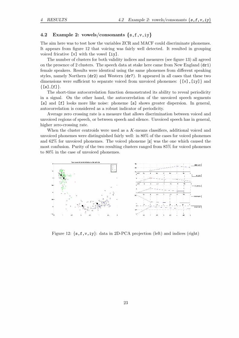
The aim here was to test how the variables ZCR and MACF could discriminate phonemes.It appears from figure 12 that voicing was fairly well detected. It resulted in groupingvoiced fricative [v] with the vowel [iy].

The number of clusters for both validity indices and measures (see figure 13) all agreedon the presence of 2 clusters. The speech data at stake here came from New England (dr1)female speakers. Results were identical using the same phonemes from different speakingstyles, namely Northern (dr2) and Western (dr7). It appeared in all cases that these twodimensions were sufficient to separate voiced from unvoiced phonemes: {[v],[iy]} and{[s],[f]}.

The short-time autocorrelation function demonstrated its ability to reveal periodicityin a signal. On the other hand, the autocorrelation of the unvoiced speech segments[s] and [f] looks more like noise: phoneme [s] shows greater dispersion. In general,autocorrelation is considered as a robust indicator of periodicity.

Average zero crossing rate is a measure that allows discrimination between voiced andunvoiced regions of speech, or between speech and silence. Unvoiced speech has in general,higher zero-crossing rate.

When the cluster centroids were used as a K-means classifiers, additional voiced andunvoiced phonemes were distinguished fairly well: in 80% of the cases for voiced phonemesand 62% for unvoiced phonemes. The voiced phoneme [z] was the one which caused themost confusion. Purity of the two resulting clusters ranged from 85% for voiced phonemesto 80% in the case of unvoiced phonemes.

Figure 12: {s,f,v,iy}: data in 2D-PCA projection (left) and indices (right)

23

4.3 Example 3: front/open vowels {ae,ah,aa} 4 RESULTS

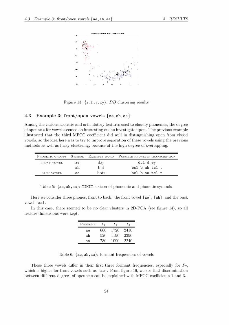
Figure 13: {s,f,v,iy}: DB clustering results

4.3 Example 3: front/open vowels {ae,ah,aa}

Among the various acoustic and articulatory features used to classify phonemes, the degreeof openness for vowels seemed an interesting one to investigate upon. The previous exampleillustrated that the third MFCC coefficient did well in distinguishing open from closedvowels, so the idea here was to try to improve separation of these vowels using the previousmethods as well as fuzzy clustering, because of the high degree of overlapping.

Phonetic groups Symbol Example word Possible phonetic transcription

front vowel ae day dcl d ey

ah but bcl b ah tcl t

back vowel aa bott bcl b aa tcl t

Table 5: {ae,ah,aa}: TIMIT lexicon of phonemic and phonetic symbols

Here we consider three phones, front to back: the front vowel [ae], [ah], and the backvowel [aa].

In this case, there seemed to be no clear clusters in 2D-PCA (see figure 14), so allfeature dimensions were kept.

Phoneme F1 F2 F3

ae 660 1720 2410ah 520 1190 2390aa 730 1090 2240

Table 6: {ae,ah,aa}: formant frequencies of vowels

These three vowels differ in their first three formant frequencies, especially for F2,which is higher for front vowels such as [ae]. From figure 16, we see that discriminationbetween different degrees of openness can be explained with MFCC coefficients 1 and 3.

24

4 RESULTS 4.3 Example 3: front/open vowels {ae,ah,aa}

Figure 14: {ae,ah,aa}: feature data in 2D-PCA

The recommended number of clusters by the Ifuz index was 2. Figure 15 displays theclustering results. The histogram on the left indicates how each phoneme was clustered:Phonemes [ae] and [aa] were clustered separately with recall values of 95%. The his-togram on the right hand side shows the content of both clusters: precision remains ratherlow since [ah] is present in both clusters. This resulted in a global purity of 70% for theentire clustering. When phoneme [ah] was not considered, separation between front andback vowels [ae] and [aa] was good: 95% correct clustering and the classifier was ableto separate additional phones pronounced by different speakers of the same sex with anefficiency of over 90%.

Figure 15: {ae,ah,aa}: content of the clusters

25

4.4 Example 4: fricatives {s,z,v,f} 4 RESULTS

Figure 16: {ae,ah,aa}: principal comp. correlation with feature dimensions

4.4 Example 4: fricatives {s,z,v,f}

The aim here was to discriminate fricatives and see which features differentiate them inorder of appearance. Formant transitions at vowel-consonant boundaries may be crucialin identifying the consonant. Since, for many consonants, such transitions are very rapid,they do not occupy many frames. This led to extracting consonants which were borderedby similar vowels (open to be more specific).

Figure 17: {s,z,v,f}: feature data in 2D-PCA

Linear correlations were weak in this case, correlation coefficient values remained below80% (see figure 18). Distinction along factor 1 between [v] and the other three phonemes,in other words in terms of voicing, was due to (MACF+ZCR) as well as (MFCC coefficients1 and 7). Factor 2 was mostly correlated to energy and MFCC coefficient 4. This factor

26

4 RESULTS 4.4 Example 4: fricatives {s,z,v,f}

was able to distinguish between labio-dentals [v],[f] from [s],[z], which are not.

Figure 18: {s,z,v,f}: principal comp. correlation with feature dimensions

Indexes Recommended K

DB 2I 3

Ifuz 3

Measures

Fmeas 3ρ 3

Table 7: {s,z,v,f}: Best K for each index and measure

Crisp and fuzzy indexes all recommended 2 or 3 clusters (see table 7). Constraint-based clustering, using fuzzy K-means with the Ifuz index and a threshold at 80% on themembership values reduced the co-articulation effect between feature vectors from differentphonemes, at vowel-consonant transitions for example. This procedure also increasedcluster quality in terms of precision, recall and purity, as depicted in histograms fromfigure 19. The top figures display clustering results according to the I index and thebottom figures correspond to results for Ifuz with the rejection criterion. The rejectedfeature points are grouped under rej in the histograms. Clustering results for phoneme[z] for instance were improved using this method. Clusters showed to be more precisewith respect to the phoneme they best represented: cluster 3 captured more [f] in thefuzzy method that it did in it crisp counterpart.

When displayed in Wavesurfer, cluster assignments were stable in time. The beginningof the spectrum corresponding to sentence si2036 is displayed in figure 20. The wordsare ”as his feet”. In figure 21, each line indicates the assignments according to crisp

27

4.4 Example 4: fricatives {s,z,v,f} 4 RESULTS

Figure 19: {s,z,v,f}: crisp (top) and fuzzy (bottom) clustering results

Figure 20: {s,z,v,f}: speech spectrum for si2036

Z Z F S

DBI

I fuz

Figure 21: {s,z,v,f}: cluster assignments in time for si2036

28

4 RESULTS 4.4 Example 4: fricatives {s,z,v,f}

partitioning using the DB and I indexes for the first two and according to Ifuz with athreshold on the membership values set at 80%. The numbers correspond to the clusterassignments and 0 stands for points which were not considered for the experiment, orrejected in the fuzzy case.

All three results indicate that phonemes [s] and [z]were not distinguished. Increasingthe number of clusters did not yield better results.

DB recommends two clusters and assigns [z] and [f] in cluster 1 and transitionfeature vectors in 2. I on the other hand recommends three which makes it possibleto differentiate the two (1 for [z] and 3 for [f], whereas 2 corresponds to transitionfeature vectors). The fuzzy method rejected many feature vectors in phone to phonetransitions (clustered as 0). Consider phoneme [f] and its transition with phoneme [iy]:figure 21 shows the co-articulation effect which the fuzzy method was able to detect. Italso resulted in eliminating points which laid on the borders in the transition [z]→ [ix]

→ [z]. Figure 20 shows the continuous variations in the spectrum, which makes theborders between phonemes hard to define.

Phoneme grave voiced continuant strident

s − − + +z − + + +v + + − −f + − + +

Table 8: {s,z,v,f}: Binary feature classification

Jackobson and Halle’s binary feature classification for the phonemes is displayed intable 8. All other features features were identical. Clustering results indicate a possibleranking of the features. [v] was the easiest to separate because of [+voiced]. Then came[f], which, unlike [s] and [z], is [+grave]. Though [z] is also considered as voiced,the spectrum from figure 20 shows that this property is not very pronounced in English.From the binary feature point of view, there is no difference between [z] and [s], whichwould explain why it was impossible to distinguish the two when using clustering methods.However, other attempts to rank different features which did not comprise [+voiced] didnot always yield the same rankings. Perhaps an average ranking can be performed overseveral sets, but the methods used here are not suitable.

29

5 DISCUSSION

5 Discussion

Visualization of the data using PCA indicated that phonetic clusters overlapped strongly,but that broad phonetic classes could be clustered well. In addition, when phonemesfrom a given broad phonetic class (e.g.: fricatives) were clustered, the most discriminativedimensions were energy, (zero-crossing rate + maximum of the autocorrelation function +a few MFCC coefficients), and clustering using only these dimensions sometimes yieldedsimilar results. Interpretation of the MFCC coefficients remained difficult.

The algorithms used in the experiments were able to cluster some of the overlappingbroad phonetic classes and distinctive binary features. In order to reduce dependencyon initialization, GMMs using the EM algorithm were used prior to K-means and theclusterings were more stable than without this procedure over different runs.

Cluster assignments were relatively stable in time for a given speaker. Fuzzy K -meanscoupled with Ifuz were able to detect co-articulation effects on the feature vectors. It islikely though, that using ∆-MFCC would have made it possible in a simpler way.

Indexes did not yield the number of phonemes. However, the Ifuz index often recom-mended the same number of clusters as the Fmeas. In most experiments, broad phoneticclasses (e.g.: stops, fricatives, open/closed vowels, etc.) were fairly captured by the clus-tering methods used.

Fmeas remained below 70% in most cases. This measure describes how well K -meansclustering can fit the classification and, considering the number of outliers, 70% is perhapsa good result. In addition, Fmeas and purity were often maximized for the same numberof clusters. In other words, the optimal value for the number of clusters k is such thatthe clustering has the best average precision and recall over all other clusterings, and itsclusters redefine the classification as well as possible with this method.

On the whole, the methods used in this report were relatively simple but were able toillustrate articulatory and acoustic differences of phonemes, and did fairly well in com-puting classifiers. It is difficult however to conclude that this procedure conducted for thevarious experiments would work well in general.

More data for one speaker would be recommendable. Though the recorded TIMIT

speech was read and that speakers had identical sex and dialect region, speaker variabilitywas also accountable for the overlapping of the clusters.

Perhaps the phonetic clusters do not exactly have the sought convex shapes, say chain-like shapes for instance. Support Vector Clustering could better deal with outliers andoverlapping clusters, without assuming the sizes and shapes of the clusters it is supposedto find. Also, the metric used here was the plain Euclidean distance. A different metricshould also we tested: for example one determined by the covariance matrices of thedetermined clusters.

30

6 CONCLUSION AND FURTHER WORK

6 Conclusion and further work

An attempt to rank all 14 binary features from Jackobson and Halle’s classification shouldbe performed. Hierarchical tree clustering could possibly create it. We have seen thatprincipal component analysis illustrated that certain feature dimensions had a strongerdiscrimative power than others for phoneme distinction. Unfortunately, this method ismore descriptive than it actually helps in deciding which phoneme a feature vector repre-sents. It is likely that discriminative analysis would be more suitable in this case.

For example, one could compare phonemes that differ by a reduced number of binaryfeatures in order to rank them by discriminative power. This would produce a set ofpairwise rankings. Then in order to perform a global ranking, we could seek an optimalranking that represents as much the partial ones as possible. Discriminative analysis wouldalso allow one to reduce the number of features from Jackobson’s classification to thosewho create a significative difference between phonemes.

This procedure could give an insight as to which characteristics of phonemes childrenfirst learn to differentiate as they learn to speak. Moreover, it would be interesting tocluster baby speech into groups of patterns of phonemes and study the level of phoneticfeature discrimination of the child’s speech.

31

REFERENCES REFERENCES

References

[1] D. Anguita, S. Ridella, F. Rivieccio, and R. Zunino. Unsupervised clustering and thecapacity of support vector machines. In Proc. of the IEEE Int. Joint Conf. on Neural

Networks, 2004.

[2] A. Ben-Hur, D. Horn, H. Siegelmann, and V. Vapnik. Support vector clustering.Journal of Machine Learning Research, 2:125–137, 2001.

[3] R. O. Duda, P. E. Hart, and D. G. Stork. Pattern Classification. Wiley-IntersciencePublication, 2000.

[4] V. Estivill-Castro. Why so many clustering algorithms: a position paper. SIGKDD

Explorations, 4(1):65–75, 2002.

[5] M. Halkidi, Y. Batistakis, and M. Vazirgiannis. Clustering algorithms and validitymeasures. IEEE Transactions on pattern analysis and machine intelligence, 24(12),2002.

[6] M. Halkidi, Y. Batistakis, and M. Vazirgiannis. Clustering validity checking methods:part ii. SIGMOD Rec., 31(3):19–27, 2002.

[7] L. Hyman. Phonology: Theory and Analysis, chapter 3. New York: Holt, Rinehartand Winston, 1975.

[8] J. Jantzen. Neurofuzzy modelling. Technical Report 98-H-874, Technical Universityof Denmark: Oersted-DTU, 1998.

[9] U. Maulik and S. Bandyopadhyay. Performance evaluation of some clustering algo-rithms and validity indices. IEEE Transactions on Pattern Analysis and Machine

Intelligence, 24(12), 2002.

[10] M. Meila and D. Hecherman. An experimental comparison of model-based clusteringmethods. Microsoft Research, Machine Learning, 42:9–29, 2001.

[11] G. Milligan and M. Cooper. An examination of indexes for determining the numberof clusters in a data set. Psychometrika, 50:159–179, 1985.

[12] G. Richard. Traitement de la parole. ENST, brique PAMU, 2003.

[13] M. Rosell, V. Kann, and J.-E. Litton. Comparing comparisons : Document clusteringevaluation using two manual classifications. In ICON, 2004.

[14] B. Stein, S. Meyer, and F. Wissbrock. On cluster validity and the information need ofusers. In Third International Conference on Artificial Intelligence and Applications,pages 216–221, 2003.

[15] M.-C. Su. A new index of cluster validity. presentation, National Central Universityof Taiwan, 2004.

[16] A. Ultsch and C. Vetter. Self-organizing feature maps versus statistical clusteringmethods. Technical Report 0994, Universiy of Marburg, 2001.

32