HAL Id: hal-01586010https://hal.archives-ouvertes.fr/hal-01586010

Submitted on 12 Sep 2017

HAL is a multi-disciplinary open accessarchive for the deposit and dissemination of sci-entific research documents, whether they are pub-lished or not. The documents may come fromteaching and research institutions in France orabroad, or from public or private research centers.

L’archive ouverte pluridisciplinaire HAL, estdestinée au dépôt et à la diffusion de documentsscientifiques de niveau recherche, publiés ou non,émanant des établissements d’enseignement et derecherche français ou étrangers, des laboratoirespublics ou privés.

Climate change: The 2015 Paris Agreement thresholdsand Mediterranean basin ecosystems

Joel Guiot, Wolfgang Cramer

To cite this version:Joel Guiot, Wolfgang Cramer. Climate change: The 2015 Paris Agreement thresholds and Mediter-ranean basin ecosystems. Science, American Association for the Advancement of Science, 2016, 354(6311), pp.465-468. �10.1126/science.aah5015�. �hal-01586010�

26. L. Overstreet Wadiche, D. A. Bromberg, A. L. Bensen,G. L. Westbrook, J. Neurophysiol. 94, 4528–4532(2005).

27. S. Ge et al., Nature 439, 589–593 (2006).28. S. Heigele, S. Sultan, N. Toni, J. Bischofberger, Nat. Neurosci.

19, 263–270 (2016).29. C. Vivar et al., Nat. Commun. 3, 1107

(2012).30. L. Madisen et al., Nat. Neurosci. 15, 793–802

(2012).31. L. Acsády, A. Kamondi, A. Sík, T. Freund, G. Buzsáki,

J. Neurosci. 18, 3386–3403 (1998).32. C. J. Magnus et al., Science 333, 1292–1296

(2011).33. T. J. Stachniak, A. Ghosh, S. M. Sternson, Neuron 82, 797–808

(2014).34. S. Ge, C. H. Yang, K. S. Hsu, G. L. Ming, H. Song, Neuron 54,

559–566 (2007).35. A. Marín-Burgin, L. A. Mongiat, M. B. Pardi, A. F. Schinder,

Science 335, 1238–1242 (2012).

36. A. Tashiro, V. M. Sandler, N. Toni, C. Zhao, F. H. Gage, Nature442, 929–933 (2006).

37. D. Dupret et al., PLOS Biol. 5, e214 (2007).

ACKNOWLEDGMENTS

We thank S. Arber and M. Soledad Espósito for providingAAV-hM4Di and AAV-PSAM-5HT3 particles and for invaluableadvice on their use, M. C. Monzón Salinas for technical help,S. Sternson for PSEM308, B. Roth for the hM3Dq andhM4Di constructs, G. Davies Sala for preliminary experiments usingretroviral expression of hM3Dq, J. Johnson for Ascl1CreERT2 mice,S. Arber for PVCre mice, members of the A.F.S. and G. Lanuza labsfor insightful discussions, and V. Piatti for critical commentson the manuscript. D.G. and A.F.S. are investigators of the ConsejoNacional de Investigaciones Científicas y Técnicas (CONICET).Supported CONICET fellowships (D.D.A., S.M.Y., M.F.T., andS.G.T.), Howard Hughes Medical Institute SIRS grant 55007652(A.F.S.), Argentine Agency for the Promotion of Science andTechnology grant PICT2013-1685, and NIH grant FIRCA

R03TW008607-01. The data reported in this manuscript aretabulated in the main paper and the supplementary materials.Author contributions: D.D.A. and D.G. contributed to the concept,designed and performed the experiments, analyzed the data,and wrote the manuscript; S.M.Y. and S.G.T. performedelectrophysiological recordings and analyzed the data; M.F.T. andK.A.B. contributed to experiments involving enriched environmentand analyzed the data; N.B. prepared retroviruses; and A.F.S.contributed to the concept, designed the experiments, analyzedthe data, wrote the manuscript, and provided financial support.

SUPPLEMENTARY MATERIALS

www.sciencemag.org/content/354/6311/459/suppl/DC1Materials and MethodsFigs. S1 to S7References (38–41)

14 January 2016; accepted 16 September 201610.1126/science.aaf2156

CLIMATE CHANGE

Climate change: The 2015 ParisAgreement thresholds andMediterranean basin ecosystemsJoel Guiot1* and Wolfgang Cramer2

The United Nations Framework Convention on Climate Change Paris Agreement ofDecember 2015 aims to maintain the global average warming well below 2°C above thepreindustrial level. In the Mediterranean basin, recent pollen-based reconstructions of climateand ecosystem variability over the past 10,000 years provide insights regarding theimplications of warming thresholds for biodiversity and land-use potential. We comparescenarios of climate-driven future change in land ecosystems with reconstructed ecosystemdynamics during the past 10,000 years. Only a 1.5°C warming scenario permits ecosystems toremain within the Holocene variability. At or above 2°C of warming, climatic change willgenerate Mediterranean land ecosystem changes that are unmatched in the Holocene, aperiod characterized by recurring precipitation deficits rather than temperature anomalies.

The United Nations Framework Conven-tion on Climate Change (UNFCCC) ParisAgreement of December 2015 aims “tohold the increase in the global averagetemperature to below 2°C above prein-

dustrial levels and to pursue efforts to limit thetemperature increase to 1.5°C.…” For many re-gions of the world, achieving the global 2°Ctarget would still imply substantially higher av-erage temperatures, with daily maxima reach-ing extreme values (1). Recent ~1°C warminghas caused damage in many systems alreadytoday (2). The degree to which future damagecould be avoided by ambitious warming thresh-olds is uncertain. Regional temperatures in the

Mediterranean basin are now ~1.3°C higher thanduring 1880–1920, compared with an increase of~0.85°C worldwide (Fig. 1). The difference be-tween (global) warming of 1.5° and >2°C abovepreindustrial levels is critically important foradaptation policies in the Mediterranean region,notably with respect to land-use systems and theconservation of biodiversity. Simulations with im-pact models have shed some light on the risksand sensitivities to climate change, but they facelimitations when applied at the regional scaleand for low levels of warming (3).To assess the regional effects of different Paris

Agreement thresholds for theMediterranean ba-sin, the Holocene reconstruction of spatiotemporalecosystem dynamics from pollen allows the de-velopment of reliable scenarios of climate-drivenchange in land ecosystems (4). Despite the effectsof human land use, broader-scale past ecosystemdynamics have been mostly driven by regionalclimate change.Mediterranean basin ecosystems are a hot

spot of the world’s biodiversity (5) and supplynumerous services to people, including clean

water, flood protection, carbon storage, and re-creation. Thus, the broad-scale vulnerability ofecosystems to climate change can be used asan indicator of the importance of the warmingthresholds identified by the Paris Agreementfor the environment and human well-being. Giv-en the confidence with which past ecosystemsand climate change can be reconstructed fromnumerous pollen profiles, the development andvalidation of more reliable numerical models forthe ecosystem-climate relationship have becomepossible. We apply such an approach to futureclimate conditions, using simulations from theCoupled Model Intercomparison Project phase5 (CMIP5) for three different greenhouse gas(GHG) forcings [see table S2 and (6) for details].An analysis of the annual mean temperatures forthese three scenarios for all climate models atthe global and Mediterranean scale, an obser-vational time series, and a spatiotemporal his-torical reconstruction at the Mediterranean scale(Fig. 1) indicate that (i) the projected warmingin the Mediterranean basin exceeds the globaltrend for most simulations; (ii) the first decadeof the 21st century has already surpassed theHolocene temperature variability; (iii) the globalwarming, but also the regional warming, is ap-proximately a linear function of the CO2 con-centration; and (iv) only a few simulations provideglobal warming lower than 2°C at the end ofthe 21st century.Mediterranean land ecosystems are sensitive

not only to warming but also to changes in wa-ter availability. Even if past variations in precip-itation and their projections for the future arespatially more heterogeneous than temperaturefields (7), for most scenarios, the changes in bothfields will combine to reduce water availabilityand trigger losses of Mediterranean ecosystemsand their biodiversity during the coming decades(8–10). During the Holocene (especially in thesecond half of this epoch), periods of precipita-tion deficits have occurred, but in contrast tothe 21st-century situation, temperatures did notrise above the present average (Fig. 1) (4). Theseperiods of precipitation deficits [~6 to ~5.2, ~4.2to ~4, and ~3.1 to ~2.9 thousand years before thepresent (yr B.P.)] have been identified as possible

SCIENCE sciencemag.org 28 OCTOBER 2016 • VOL 354 ISSUE 6311 465

1Aix-Marseille Université, CNRS, Institut de Recherche pourle Développement (IRD), Collège de France, Centre Européende Recherche et d’Enseignement de Géosciencesde l’Environnement (CEREGE), Ecosystèmes Continentaux etRisques Environnementaux (ECCOREV), Aix-en-Provence,France. 2Mediterranean Institute for Biodiversity and Ecology(IMBE), Aix-Marseille Université, CNRS, IRD, AvignonUniversity, 13545 Aix-en-Provence, France.*Corresponding author. Email: guiot@cerege.fr

RESEARCH | REPORTS

on

Oct

ober

28,

201

6ht

tp://

scie

nce.

scie

ncem

ag.o

rg/

Dow

nloa

ded

from

causes of declines or collapses in civilization inthe eastern Mediterranean region (11–13). A re-cent study (14) has attributed important cropfailures in Syria to two strong drought episodes—characterized by a lack of precipitation (reducedby up to 30% in the 6-month winter season) andhigh temperatures (warming of 0.5° to 1.0°C inthe annual mean relative to the 20th-centuryaverage)—in the eastern Mediterranean between1998 and 2010. The 1998–2012 period was thedriest of the last 500 years (15). Even if societal

factors have likely been the primary causes ofthese crises (16, 17), Holocene droughts and theassociated variability in land productivity mayhave also played a role, indicating the potentialeffect of climate change on agriculture-basedeconomies.To relate the past variability of climate and

ecosystems with possible future conditions, weuse the process-based ecosystem model BIOME4(6), which, when compared with correlationtechniques, allows a more reliable reconstruc-

tion of past climate-vegetation equilibria. Di-rect human impacts, such as the cultivation ofcrops or degradation processes, are not takeninto account. For the Holocene, BIOME4 wasinverted to generate gridded climate patternsby time steps of 100 years and associated eco-systems (“biomes”) from pollen records (4). Forthe future, the forward application of the samemodel yields ecosystem distributions from cli-mate projections (6). The limitations of a rel-atively simple ecosystem model are largely offsetby two factors. First, this method directly relatesthe physical environment, including its seasonalvariability, and atmospheric CO2 to plant pro-cesses and thereby avoids the strong assump-tions made by niche models (18). Second, pastobservations are analyzed with the same process-based model that is used for the future projec-tions, thus providing a more coherent frameworkfor the assessment.Figure 2 indicates reconstructed and estimated

shifts in the distribution of major Mediterraneanbiomes (temperate conifer forest, deciduous forest,warm mixed forest, xerophytic shrubland, andsteppe) over time for the past and future, relativeto their current distribution. During the Holocene,only up to 15% of the land has had differentecosystems from those existing today at anymoment. The 10% level was exceeded only dur-ing eight 100-year time slices, and all of theseperiods occurred before 4200 yr B.P. All of thesewere relatively humid periods, which becameless frequent after this date (4). The past fourmillennia, and notably the past century, weregenerally dry compared with the first half of theHolocene.The future is represented by the following

three classes of simulated time-space fields

466 28 OCTOBER 2016 • VOL 354 ISSUE 6311 sciencemag.org SCIENCE

Fig. 1. Annual temperature change (from thepreindustrial mean) versus CO2 atmosphericconcentrations. Colored boxes represent the Inter-governmental Panel on Climate Change RCP scenar-ios for 2010–2100 (25th, 50th, and 75th percentiles):RCP2.5 (green), RCP4.5 (orange), and RCP8.5 (red).Solid blue circles with vertical bars concern thesame three scenarios for the Mediterranean region(10°W to 45°E, 28°N to 48°N). For the Holocene,the blue circles with cyan error bars (1s) are derivedfrom climate reconstructions from pollen for eachcentury from 10,000 to 100 yr B.P. by steps of100 years (4) (the variability is multiplied by a factorof 3 to account for the fact that the time resolutionis 100 years instead of 10-year averages for thescenarios). The vertical bars represent the ±1 SDsprovided by the reconstruction method.The medium-sized 1901–2009 circles are the Climatic ResearchUnit TS3.1 gridded observations (20) averaged in thesame area and smoothed with a time step of 10 years.The vertical bars represent the corresponding SDs.The horizontal lines indicate the preindustrial meantemperature and the three thresholds referred to inthe Paris Agreement (1.5°, 2°, and 3°C). The blackregression line is based on the three global scenar-ios. ppmv, parts per million by volume.

Fig. 2. Proportion of grid cells with a biome change relative to the preindustrial period for theMediterranean area (10°W to 45°E, 28°N to 48°N). The horizontal axis represents the time scale,in years before the present (20th century) for the past (negative numbers) and in years after thepresent (CE 2000–2010) for the future (positive numbers). Holocene biomes (in black) are based onreconstructions from pollen data (4). Colored lines are given by the BIOME4 model as applied to theRCP projections (see text). Horizontal lines represent the 50th, 80th, 90th, and 99th percentiles of theHolocene values.The colored areas illustrate the interquartile interval provided by the intermodel variability.

RESEARCH | REPORTS

on

Oct

ober

28,

201

6ht

tp://

scie

nce.

scie

ncem

ag.o

rg/

Dow

nloa

ded

from

of temperature and rainfall, which are derivedfrom the CMIP5 project (table S2): Represent-ative Concentration Pathway 8.5 (RCP8.5) (22simulations), RCP4.5 (23 simulations), and RCP2.6(16 simulations). RCP2.6 approximates the 2°Ctarget. To assess the 1.5°C target, we created afourth class (denoted RCP2.6L) from selectedCMIP5 scenarios [see (6) for details]. Up to2030, all four classes generate similar ecosystemdistributions and generally remain within thebounds of Holocene fluctuations. By the end ofthe 21st century, RCP2.6L remains in the rangeof the 80th and 99th percentiles of the Holo-cene, whereas RCP2.6 simulates Mediterranean

ecosystems as they were during the most extremeperiod of the Holocene (at 4700 yr B.P.), with achange of 12 to 15%.The limits of the Mediterranean vegetation

types defined by biogeographers (19) broadlycoincide with our simulated warm mixed forestbiome (Fig. 3A), with the following two excep-tions: (i) Simulated warm mixed forests also ex-tend to the Atlantic Ocean in the west of France,indicating the inability of BIOME4 to distinguishAtlantic pine forests, and (ii) the narrow strip ofMediterranean vegetation on the Libyan andEgyptian coast, which is below the spatial reso-lution of our climatic data. The reconstruction

for the period of the Holocene (4700 yr B.P.) (Fig.3B) with the greatest difference from today (Fig.3A) shows that the main differences are relatedto the further regression of forested areas in thesouthern Mediterranean associated with expand-ing desert areas.Simulations for the RCP2.6L and RCP2.6 sce-

narios do not change biome distributions muchat the end of the 21st century (Fig. 3, D to E).However, for the same period, the RCP4.5 sce-nario induces desert extension toward NorthAfrica, the regression of alpine forests, andthe extension of Mediterranean sclerophyllousvegetation. Under the RCP8.5 scenario, all of

SCIENCE sciencemag.org 28 OCTOBER 2016 • VOL 354 ISSUE 6311 467

Fig. 3. Mediterranean biome maps. Distribution of Mediterranean biomes (A) reconstructed (rec) from pollen for the present; (B) reconstructed from pollenfor 4700 yr B.P.; (C) simulated by the BIOME4 model for the present; and (D to G) for scenarios RCP2.6L, RCP2.6, RCP4.5, and RCP8.5, respectively, at theend of the 21st century. For the simulations, each point indicates the most frequent biome in the ensemble of CMIP5 climate simulations. Map (H) indicates, foreach point, the number of scenarios different from the simulated present. Yellow areas indicate when only RCP8.5 is different; orange areas denote whenRCP4.5 and RCP8.5 are different; red areas indicate when RCP2.6, RCP4.5, and RCP8.5 are different; and blue circles mark areas in which the biome type at4700 yr B.P. is different from the present biome type.

RESEARCH | REPORTS

on

Oct

ober

28,

201

6ht

tp://

scie

nce.

scie

ncem

ag.o

rg/

Dow

nloa

ded

from

southern Spain turns into desert, deciduousforests invade most of the mountains, and Me-diterranean vegetation replaces most of thedeciduous forests in a large part of the Mediter-ranean basin. Figure 3H illustrates the variationfrom areas without any changes, regardless ofscenario (stable white areas), to areas in whichchanges from scenario RCP2.6 already appear(red areas). As expected, the most-sensitive areasare those located at the limit between two biomes—for example, in the mountains at the transitionbetween temperate and montane forest or in thesouthern Mediterranean at the transition betweenforest and desert biomes. The map for 4700 yrB.P., in which the past changes were among thehighest (Fig. 3B), has the largest changes in thesouthwest, eastern steppe areas, and the moun-tains, but these changes are relatively sparse.Our analysis shows that, in approximately one

century, anthropogenic climate change withoutambitious mitigation policies will likely alterecosystems in the Mediterranean in a way thatis without precedent during the past 10 millen-nia. Despite known uncertainties in climatemodels, GHG emission scenarios at the levelof country commitments before the UNFCCCParis Agreement will likely lead to the sub-stantial expansion of deserts in much of south-ern Europe and northern Africa. The highlyambitious RCP2.6 scenario seems to be the onlypossible pathway toward more limited impacts.Only the coldest RCP2.6L simulations, whichcorrespond broadly to the 1.5°C target of theParis Agreement, allow ecosystem shifts to re-main inside the limits experienced during theHolocene.This analysis does not account for other hu-

man impacts on ecosystems, in addition to cli-mate change (i.e., land-use change, urbanization,soil degradation, etc.), which have grown inimportance after the mid-Holocene and havebecome dominant during the past centuries.Many of these effects are likely to become evenstronger in the future because of the expand-ing human population and economic activity.Most land change processes reduce natural veg-etation or they seal or degrade the soils, repre-senting additional effects on ecosystems, whichwill enhance, rather than dampen, the biomeshifts toward a drier state than estimated bythis analysis. This assessment shows that, with-out ambitious climate targets, the potential forfuture managed or unmanaged ecosystems tohost biodiversity or deliver services to society islikely to be greatly reduced by climate changeand direct local effects.

REFERENCES AND NOTES

1. S. I. Seneviratne, M. G. Donat, A. J. Pitman, R. Knutti,R. L. Wilby, Nature 529, 477–483 (2016).

2. W. Cramer et al., in Climate Change 2014: Impacts, Adaptation,and Vulnerability. Part A: Global and Sectoral Aspects.Contribution of Working Group II to the Fifth Assessment Reportof the Intergovernmental Panel on Climate Change, C. B. Fieldet al., Eds. (Cambridge Univ. Press, 2014), pp. 979–1037.

3. C.-F. Schleussner et al., Earth Syst. Dyn. Discuss. 6,2447–2505 (2015).

4. J. Guiot, D. Kaniewski, Front. Earth Sci. 3, 28 (2015).

5. F. Médail, N. Myers, in Hotspots Revisited: Earth’s BiologicallyRichest and Most Endangered Terrestrial Ecoregions,R. A. Mittermeier et al., Eds. (Conservation International,2004), pp. 144–147.

6. Materials and methods are available as supplementarymaterials on Science Online.

7. E. Xoplaki, J. F. González-Rouco, J. Luterbacher, H. Wanner,Clim. Dyn. 23, 63–78 (2004).

8. L. Maiorano et al., Philos. Trans. R. Soc. London Ser. B 366,2681–2692 (2011).

9. T. Keenan, J. Maria Serra, F. Lloret, M. Ninyerola, S. Sabate,Glob. Change Biol. 17, 565–579 (2011).

10. W. Thuiller, S. Lavorel, M. B. Araújo, Glob. Ecol. Biogeogr. 14,347–357 (2005).

11. B. Weninger et al., Doc. Praehist. 36, 7–59(2009).

12. D. Kaniewski, E. Van Campo, H. Weiss, Proc. Natl. Acad. Sci.U.S.A. 109, 3862–3867 (2012).

13. N. Roberts, D. Brayshaw, C. Kuzucuoglu, R. Perez, L. Sadori,Holocene 21, 3–13 (2011).

14. C. P. Kelley, S. Mohtadi, M. A. Cane, R. Seager, Y. Kushnir,Proc. Natl. Acad. Sci. U.S.A. 112, 3241–3246 (2015).

15. B. I. Cook, K. J. Anchukaitis, R. Touchan, D. M. Meko,E. R. Cook, J. Geophys. Res. 121, 2060–2074 (2016).

16. G. Middleton, J. Archaeol. Res. 20, 257–307 (2012).17. A. B. Knapp, S. W. Manning, Am. J. Archaeol. 120, 99–149

(2016).18. C. B. Yackulc, J. D. Nichols, J. Reid, R. Der, Ecology 96, 16–23

(2015).19. C. Roumieux et al., Ecol. Mediterr. 36, 17–24

(2010).20. I. Harris, P. D. Jones, T. J. Osborn, D. H. Lister, Int. J. Climatol.

34, 623–642 (2014).

ACKNOWLEDGMENTS

The authors are members of the Observatoire des Sciences del’Univers Pytheas Institute and the ECCOREV network. Thisresearch has been funded by Labex OT-Med (project ANR-11-LABEX-0061), the “Investissements d’Avenir” French governmentproject of the French National Research Agency (ANR),AMidex (project 11-IDEX-0001-02), and the EuropeanUnion FP7-ENVIRONMENT project OPERAs (grant 308393).We acknowledge the World Climate Research Programme’sWorking Group on Coupled Modelling, which is responsible forCMIP, and we thank the climate modeling groups (table S2) forproducing and making their model outputs available. For CMIP,the U.S. Department of Energy’s Program for Climate ModelDiagnosis and Intercomparison provides coordinating supportand led the development of software infrastructure, inpartnership with the Global Organization for Earth SystemScience Portals. R. Suarez and S. Shi have extracted andpreprocessed the model simulations. Holocene climatereconstructions are available at http://database.otmed.fr/geonetworkotmed/srv/eng/search - |54b9bf34-57ae-45ea-b455-9f90351e538f. Future climate projections are available athttp://cmip-pcmdi.llnl.gov/cmip5/.

SUPPLEMENTARY MATERIALS

www.sciencemag.org/content/354/6311/465/suppl/DC1Materials and MethodsTable S1 and S2References (21–28)

6 July 2016; accepted 21 September 201610.1126/science.aah5015

GENE EXPRESSION

Xist recruits the X chromosome to thenuclear lamina to enablechromosome-wide silencingChun-Kan Chen,1 Mario Blanco,1 Constanza Jackson,1 Erik Aznauryan,1

Noah Ollikainen,1 Christine Surka,1 Amy Chow,1 Andrea Cerase,2

Patrick McDonel,3 Mitchell Guttman1*

The Xist long noncoding RNA orchestrates X chromosome inactivation, a process that entailschromosome-wide silencing and remodeling of the three-dimensional (3D) structure of theX chromosome. Yet, it remains unclear whether these changes in nuclear structure aremediated by Xist and whether they are required for silencing. Here, we show that Xist directlyinteracts with the Lamin B receptor, an integral component of the nuclear lamina, and thatthis interaction is required for Xist-mediated silencing by recruiting the inactive X to thenuclear lamina and by doing so enables Xist to spread to actively transcribed genes acrossthe X. Our results demonstrate that lamina recruitment changes the 3D structure of DNA,enabling Xist and its silencing proteins to spread across the X to silence transcription.

The Xist long noncoding RNA (lncRNA) ini-tiates X chromosome inactivation (XCI), aprocess that entails chromosome-wide tran-scriptional silencing (1) and large-scale re-modeling of the three-dimensional (3D)

structure of the X chromosome (2–4), by spread-ing across the future inactive X chromosomeand excluding RNA polymerase II (PolII) (1, 5).Xist initially localizes to genomic DNA regionson the X chromosome that are not actively tran-scribed (6–8), before spreading to actively tran-scribed genes (7–9). Deletion of a highly conservedregion of Xist that is required for transcrip-

tional silencing, called the A-repeat (10), leads toa defect in Xist spreading (7) and spatial ex-clusion of active genes from the Xist-coated nu-clear compartment (9). Whether these structuralchanges are required for, or merely a conse-quence of, transcriptional silencing mediatedby the A-repeat of Xist remains unclear (7, 9).Recently, we and others identified by meansof mass spectrometry the proteins that inter-act with Xist (11–13). One of these proteins isthe Lamin B receptor (LBR) (11, 13), a trans-membrane protein that is anchored in theinner nuclear membrane, binds to Lamin B,

468 28 OCTOBER 2016 • VOL 354 ISSUE 6311 sciencemag.org SCIENCE

RESEARCH | REPORTS

on

Oct

ober

28,

201

6ht

tp://

scie

nce.

scie

ncem

ag.o

rg/

Dow

nloa

ded

from

(6311), 465-468. [doi: 10.1126/science.aah5015]354Science Joel Guiot and Wolfgang Cramer (October 27, 2016) Mediterranean basin ecosystemsClimate change: The 2015 Paris Agreement thresholds and

 Editor's Summary

   

, this issue p. 465Sciencepast 10,000 years.

thelikely over the next century to produce ecosystems in the Mediterranean basin that have no analog in may persist under a 1.5°C warming above preindustrial temperature levels. A 2°C warming, however, isdifferent climate-change scenarios. Vegetation and land-use systems observed in the Holocene records information as a baseline against which to compare predictions of future climate and vegetation underMediterranean during the Holocene (the most recent ~10,000 years). Guiot and Cramer used this

Pollen cores from sediments provide rich detail on the history of vegetation and climate in theA warming limit for the Mediterranean basin

This copy is for your personal, non-commercial use only.

Article Tools

http://science.sciencemag.org/content/354/6311/465article tools: Visit the online version of this article to access the personalization and

Permissionshttp://www.sciencemag.org/about/permissions.dtlObtain information about reproducing this article:

is a registered trademark of AAAS. ScienceAdvancement of Science; all rights reserved. The title Avenue NW, Washington, DC 20005. Copyright 2016 by the American Association for thein December, by the American Association for the Advancement of Science, 1200 New York

(print ISSN 0036-8075; online ISSN 1095-9203) is published weekly, except the last weekScience

on

Oct

ober

28,

201

6ht

tp://

scie

nce.

scie

ncem

ag.o

rg/

Dow

nloa

ded

from

www.sciencemag.org/content/354/6311/465/suppl/DC1

Supplementary Materials for

Climate change: The 2015 Paris Agreement thresholds and

Mediterranean basin ecosystems

Joel Guiot* and Wolfgang Cramer

*Corresponding author. Email: guiot@cerege.fr

Published 28 October 2016, Science 354, 465 (2016)

DOI: 10.1126/science.aah5015

This PDF file includes:

Materials and Methods

Tables S1 and S2

References

2

Materials and Methods

The reconstruction of Holocene climate and biomes (4) is based on the process-based

equilibrium terrestrial biosphere model BIOME4 (21), which has been used in numerous

regional to global scale studies (22). This model predicts structure and productivity of broad-

scale land ecosystems from monthly temperature and rainfall values and annual CO2

concentration. It uses a photosynthesis scheme that simulates acclimation of plants to changed

atmospheric CO2 by optimization of nitrogen allocation to foliage and by accounting for the

effects of CO2 on net assimilation, stomatal conductance, leaf area index (LAI) and ecosystem

water balance. BIOME4 is based on sufficiently simple descriptions of ecophysiological

processes to allow broad-scale application. It represents substantial advantages over niche-

models because it has not been tuned to reproduce present-day potential vegetation, but rather

to simulate correctly the main processes underlying the potential vegetation distribution

which are assumed to have been similar throughout the Holocene. BIOME4 does not account

for human land use.

The inputs of the model are monthly average / total values of temperature, precipitation and

cloudiness percentage, atmospheric CO2 concentration, and (static) soil texture. The outputs

include net primary production (NPP) of each of the potentially occurring 13 plant functional

types (PFT), and the corresponding ‘biome type’, from a set of 28 broad categories (Table

S1). To obtain a robust classification of ecosystem types suitable for the analysis of

Mediterranean vegetation, compatible with current biogeographical knowledge of potential

natural vegetation in the region (23), the 28 biome types provided by BIOME4 were

aggregated into 11 groups (Table S1).

For the Holocene, pollen records from a large number of sources, initially percentages of a

number of taxa (which can be species, genera or families according to possibilities of

morphological differentiation), are grouped into pollen plant functional types (PFT) scores

according to the “biomization” method adapted by (24). Using these data, BIOME4 is run in

inverse mode, i.e. a large number of randomized climate conditions are tried at each time step

and for each grid cell. For each of these, the NPP of all 13 PFT’s is compared to PFT scores

calculated from pollen (4). The climate conditions for which the simulated NPP matches best

with the pollen-derived PFTs scores provide the reconstruction and hence the corresponding

biome type. The atmospheric CO2 concentration is provided by the ice cores at Taylor Dome,

Antarctica (25) and the soil parameters are kept to the present values. Since the spatio-

temporal patterns reflected by pollen diagrams are also influenced by historic land use, the

reconstruction also reflects direct human impacts on ecosystems, however this effect is

assumed to be relatively minor for most of the Holocene. Model outputs in this study are

gridded climate and biome types on a coarse grid of 2° in latitude and 4° in longitude. To

allow for direct comparison of reconstructed and projected biome patterns, we have

interpolated the reconstructions to a common 1°x1° resolution.

For future projections, we use BIOME4 in forward mode, i.e. scenarios from climate

simulations under different scenarios are used as inputs yielding the biome type generated by

this climate. We use temperature and rainfall outputs from climate models assembled in

CMIP5 (26), forced by three greenhouse gas radiative forcing (Representative Concentration

Pathways, RCP) (27). RCP8.5 (GHG radiative forcing <8.5 W/m2) is the “business as usual”

scenario. RCP4.5 corresponds to policies to maintain GHG radiative forcing below 4.5 W/m2

and approximates the effort of mitigation contained in the intended nationally determined

contributions (INDC) proposed by the governments at the Paris COP21. RCP2.6 corresponds

to more ambitious mitigation policies, with a GHG radiative forcing constrained to remain

3

below 2.6 W/m2. It is the only one able to limit the global warming to 2 °C. Constrained by

the availability of simulation outputs in the CMIP5 archive, we use between 16 and 23

simulations performed by 13 climate modeling centers (Table S2). We also use for BIOME4

the atmospheric CO2 concentrations related to these scenarios.

To correct for climate model bias and differences in spatial resolution, we use anomalies

(projection minus control) of monthly temperature and precipitation values from all

simulations. The anomalies are interpolated to a common grid of 1x1° of longitude and

latitude (2997 land grid cells for the Mediterranean basin) and then added to the present

climate normal given by the CRU TS 3.23 data file (20). Climate projections from 2010 to

2100 are used as decadal monthly averages.

The mean global temperature simulated for the last 21st century decade under the RCP2.6

scenario is about 2 °C above the pre-industrial temperature (Fig. 1). Among the simulations

available, only two keep global warming below 1.5°C throughout the 21st century. To be able

to calculate uncertainties based on realistic inter-model dispersion, we have constructed an

additional low-warming scenario with variability comparable to the three RCP groups by

selecting from all other 16 simulations those decades for which global warming happens to be

lower than 1.5 °C. Assuming that the effect of changes in time-lagged systems such as large-

scale ocean circulations are negligible (3), we adopt the following procedure: (i) for each

decade of the 21st century, we build a theoretical Gaussian probability distribution N(1.2 °C,

Sk) of the global mean temperature anomaly where Sk is the standard deviation of the 16

global temperature simulations for decade k; (ii) we then sample a large number (say 1000)

values from this distribution; (iii) each of these 1000 values is approximated by the closest

simulation from the 16 original simulations of the ten decades. This provides a set of 1000

simulations compatible with the +1.5 °C threshold called RCP2.6L, which will be used for

calculating the most probable biome in each grid cell.

BIOME4 is driven by monthly temperature and precipitation fields interpolated from climate

model simulations; the monthly cloudiness (%) fields are calculated by linear regression from

the temperature and precipitation values (28); the soil parameters are kept to the present

values. We use the CO2 atmospheric concentration time-series used by CMIP5 (27). High

levels of CO2 enable to enhance photosynthesis and to increase the water use efficiency of the

vegetation. These processes, not discussed here, are taken into account in the future

projections of biome type distribution, as they may partly compensate the increase of

evapotranspiration projected for the future. Examples of biome maps are given in Fig. 3.

To estimate the magnitude of the effect of climatic change on the aggregated 11 ecosystem

types, we calculate the number of biome type changes across the 2997 grid cells for each of

the model simulations relative to the estimated current distribution, i.e. the simulation at

2000-2010 by RCP2.6 for the future scenarios (Fig.3A) and the reconstruction based on the

CRU TS 3.23 climate field (Fig. 3E). The time-series of biome changes are given in Fig. 2:

the Holocene changes by steps of 100 years for the past (10,000 to 0 years BP) and the future

changes by steps of 10 years for the future (0 to 100 years after Present).

The uncertainties on the projections are restricted to the dispersion between the climate

simulations which are directly propagated to the proportions of biome type changes. There is

no possibility to take into account the deviations between the mean climate simulation and the

true climate, nor those between simulated and true vegetation. For the Holocene, the method

enables to calculate the uncertainties on the climate reconstructions (see the error bars for the

annual temperature in Fig. 1), but not on the biome type. We assume that the temporal

variability of the biome type changes is a better estimate of the biome uncertainty than the

within grid cell variability.

4

Fig. 3 illustrates this design. The maps have a resolution of 1°x1°. Fig. 3A is obtained from

BIOME4 inversion based on present day (last century) pollen data. Fig. 3B is obtained in the

same way for the pollen data on the 4650-4750 yr BP time slice. The grid cells where the

biome type has changed between both periods are indicated with blue circles in Fig. 3H. The

changes are mainly in Northern Africa at the interface of the desert and in the mountains areas

of Near East, Anatolia, the Balkans and the Alps. Fig. 3C represents the biome distribution

simulated by BIOME4 from present climate. The main difference with the pollen

reconstruction in Fig. 3A is that BIOME4 simulates temperate deciduous forest in many areas

where are reconstructed warm mixed forest from pollen. This is likely due to an

overrepresentation of pine pollen in pollen data. Fig. 3D, 3E, 3F and 3G are forward biome

simulations by BIOME4 from climate projections at the end of the 21st century. The four

maps shows the gradient between a “1.5 °C world” to a “4 °C world” with a progressive

extension of deserts and a regression of cool and alpine forest. This is summarized by Fig.

3H, which shows that the proportion of grid cells with a biome change is relatively low with

RCP2.6L scenario (7% in red), increasing to 13% (in orange) with RCP2.6, to 17% (in

yellow) with RCP4.5 and to 31% (in yellow) with RCP8.5.

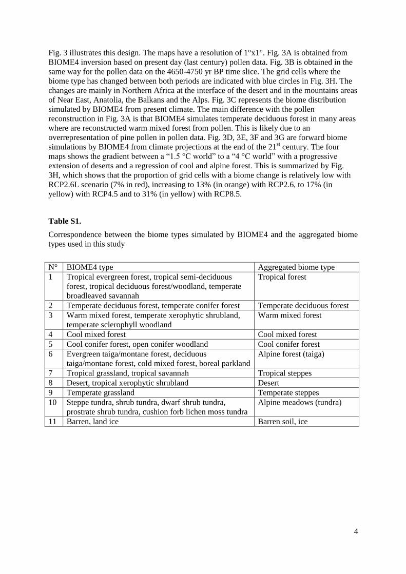
Table S1.

Correspondence between the biome types simulated by BIOME4 and the aggregated biome

types used in this study

N° BIOME4 type Aggregated biome type

1 Tropical evergreen forest, tropical semi-deciduous

forest, tropical deciduous forest/woodland, temperate

broadleaved savannah

Tropical forest

2 Temperate deciduous forest, temperate conifer forest Temperate deciduous forest

3 Warm mixed forest, temperate xerophytic shrubland,

temperate sclerophyll woodland

Warm mixed forest

4 Cool mixed forest Cool mixed forest

5 Cool conifer forest, open conifer woodland Cool conifer forest

6 Evergreen taiga/montane forest, deciduous

taiga/montane forest, cold mixed forest, boreal parkland

Alpine forest (taiga)

7 Tropical grassland, tropical savannah Tropical steppes

8 Desert, tropical xerophytic shrubland Desert

9 Temperate grassland Temperate steppes

10 Steppe tundra, shrub tundra, dwarf shrub tundra,

prostrate shrub tundra, cushion forb lichen moss tundra

Alpine meadows (tundra)

11 Barren, land ice Barren soil, ice

5

Table S2.

CMIP5 simulations (code of model, institute name); crosses indicate if the model is used for

the scenario.

Model Institute RCP2.6 RCP4.5 RCP8.5 bcc-csm1-1 Beijing Climate Center, China Meteorological Administration X X X bcc-csm1-1-m Beijing Climate Center, China Meteorological Administration X X X CanESM2 Canadian Centre for Climate modelling, Canada X X X CESM1-BGC Community Earth System Model Contributors, NSF-DOE-

NCAR, USA X

CESM1-CAM5 Community Earth System Model Contributors, NSF-DOE-

NCAR, USA X

CMCC-CM Centro Euro-Med per Cambiamenti Climatici, Italy X X CMCC-CMS Centro Euro-Med per Cambiamenti Climatici, Italy X X CMCC-CESM Centro Euro-Med per Cambiamenti Climatici, Italy X CNRM-CM5 Centre National de Recherches Météorologiques / Centre

Européen de Recherche et Formation Avancée en Calcul

Scientifique, France

X X X

GFDL-CM3 NOAA Geophysical Fluid Dynamics Laboratory, USA X X GISS-E2-H NASA Goddard Institute for Space Studies, USA X X GISS-E2-H-CC NASA Goddard Institute for Space Studies, USA X X GISS-E2-R NASA Goddard Institute for Space Studies, USA X X X GISS-E2-R-CC NASA Goddard Institute for Space Studies, USA X HadGEM2-AO Met-Office – Hadley Center, UK X X X HadGEM2-CC Met-Office – Hadley Center, UK X HadGEM2-ES Met-Office – Hadley Center, contributed by Instituto Nacional

de Pesquisas Espaciais, Spain X X

HadGEM2-ES-

CC

Met-Office – Hadley Center, contributed by Instituto Nacional

de Pesquisas Espaciais, Spain

inmcm4 Inst. For Numerical Mathematics, Russia X X IPSL-CM5A-LR Institut Pierre-Simon Laplace, France X X X IPSL-CM5A-

MR

Institut Pierre-Simon Laplace, France X X X

IPSL-CM5B-LR Institut Pierre-Simon Laplace, France X X MPI-ESM-LR Max-Planck Inst. für Meteorologie, Germany X X X MPI-ESM-MR Max-Planck Inst. für Meteorologie, Germany X X X MRI-CGCM3 Meteorological Research Institute, Japan X X X MRI-ESM1 Meteorological Research Institute, Japan X NorESM1-M Norwegian Climate Centre X X X NorESM1-ME Norwegian Climate Centre X X X

Nb

simulations

16 23 22

References and Notes

1. S. I. Seneviratne, M. G. Donat, A. J. Pitman, R. Knutti, R. L. Wilby, Allowable CO2 emissions

based on regional and impact-related climate targets. Nature 529, 477–483

(2016).doi:10.1038/nature16542 Medline

2. W. Cramer et al., in Climate Change 2014: Impacts, Adaptation, and Vulnerability. Part A:

Global and Sectoral Aspects. Contribution of Working Group II to the Fifth Assessment

Report of the Intergovernmental Panel on Climate Change, C. B. Field et al., Eds.

(Cambridge Univ. Press, 2014), pp. 979–1037.

3. C.-F. Schleussner, T. K. Lissner, E. M. Fischer, J. Wohland, M. Perrette, A. Golly, J. Rogelj,

K. Childers, J. Schewe, K. Frieler, M. Mengel, W. Hare, M. Schaeffer, Differential

climate impacts for policy-relevant limits to global warming: The case of 1.5°C and 2°C.

Earth Syst. Dyn. Discuss. 6, 2447–2505 (2015). doi:10.5194/esdd-6-2447-2015

4. J. Guiot, D. Kaniewski, The Mediterranean Basin and Southern Europe in a warmer world:

What can we learn from the past? Front. Earth Sci. 3, 28 (2015).

doi:10.3389/feart.2015.00028

5. F. Médail, N. Myers, in Hotspots Revisited: Earth’s Biologically Richest and Most

Endangered Terrestrial Ecoregions, R. A. Mittermeier et al., Eds. (Conservation

International, 2004), pp. 144–147.

6. Materials and methods are available as supplementary materials on Science Online.

7. E. Xoplaki, J. F. González-Rouco, J. Luterbacher, H. Wanner, Wet season Mediterranean

precipitation variability: Influence of large-scale dynamics and trends. Clim. Dyn. 23, 63–

78 (2004). doi:10.1007/s00382-004-0422-0

8. L. Maiorano, A. Falcucci, N. E. Zimmermann, A. Psomas, J. Pottier, D. Baisero, C. Rondinini,

A. Guisan, L. Boitani, The future of terrestrial mammals in the Mediterranean basin

under climate change. Philos. Trans. R. Soc. London Ser. B 366, 2681–2692

(2011).doi:10.1098/rstb.2011.0121 Medline

9. T. Keenan, J. Maria Serra, F. Lloret, M. Ninyerola, S. Sabate, Predicting the future of forests

in the Mediterranean under climate change, with niche- and process-based models: CO2

matters! Glob. Change Biol. 17, 565–579 (2011). doi:10.1111/j.1365-2486.2010.02254.x

10. W. Thuiller, S. Lavorel, M. B. Araújo, Niche properties and geographical extent as predictors

of species sensitivity to climate change. Glob. Ecol. Biogeogr. 14, 347–357 (2005).

doi:10.1111/j.1466-822X.2005.00162.x

11. B. Weninger, L. Clare, E. Rohling, O. Bar-Yosef, U. Böhner, M. Budja, M. Bundschuh, A.

Feurdean, H. G. Gebe, O. Jöris, J. Linstädter, P. Mayewski, T. Mühlenbruch, A.

Reingruber, G. Rollefson, D. Schyle, L. Thissen, H. Todorova, C. Zielhofer, The impact

of rapid climate change on prehistoric societies during the Holocene in the Eastern

Mediterranean. Doc. Praehist. 36, 7–59 (2009). doi:10.4312/dp.36.2

12. D. Kaniewski, E. Van Campo, H. Weiss, Drought is a recurring challenge in the Middle East.

Proc. Natl. Acad. Sci. U.S.A. 109, 3862–3867 (2012).doi:10.1073/pnas.1116304109

Medline

13. N. Roberts, D. Brayshaw, C. Kuzucuoglu, R. Perez, L. Sadori, The mid-Holocene climatic

transition in the Mediterranean: Causes and consequences. Holocene 21, 3–13 (2011).

doi:10.1177/0959683610388058

14. C. P. Kelley, S. Mohtadi, M. A. Cane, R. Seager, Y. Kushnir, Climate change in the Fertile

Crescent and implications of the recent Syrian drought. Proc. Natl. Acad. Sci. U.S.A. 112,

3241–3246 (2015).doi:10.1073/pnas.1421533112 Medline

15. B. I. Cook, K. J. Anchukaitis, R. Touchan, D. M. Meko, E. R. Cook, Spatiotemporal drought

variability in the Mediterranean over the last 900 years. J. Geophys. Res. 121, 2060–2074

(2016). doi:10.1002/2015JD023929

16. G. Middleton, Nothing lasts forever: Environmental discourses on the collapse of past

societies. J. Archaeol. Res. 20, 257–307 (2012). doi:10.1007/s10814-011-9054-1

17. A. B. Knapp, S. W. Manning, Crisis in context: The end of the Late Bronze Age in the

Eastern Mediterranean. Am. J. Archaeol. 120, 99–149 (2016). doi:10.3764/aja.120.1.0099

18. C. B. Yackulc, J. D. Nichols, J. Reid, R. Der, To predict the niche, model colonization and

extinction. Ecology 96, 16–23 (2015).doi:10.1890/14-1361.1 Medline

19. C. Roumieux et al., Actualisation des limites de l’aire du bioclimat méditerranéen selon les

critères de Daget (1977). Ecol. Mediterr. 36, 17–24 (2010).

20. I. Harris, P. D. Jones, T. J. Osborn, D. H. Lister, Updated high-resolution grids of monthly

climatic observations - the CRU TS3.10 dataset. Int. J. Climatol. 34, 623–642 (2014).

doi:10.1002/joc.3711

21. J. O. Kaplan et al., Climate change and Arctic ecosystems: 2. Modeling, paleodata-model

comparisons, and future projections. J. Geophys. Res. 108, 8171 (2003).

doi:10.1029/2002JD002559

22. S. P. Harrison, C. I. Prentice, Climate and CO2 controls on global vegetation distribution at

the Last Glacial Maximum: Analysis based on paleovegetation data, biome modelling

and paleoclimate simulations. Glob. Change Biol. 9, 983–1004 (2003).

doi:10.1046/j.1365-2486.2003.00640.x

23. J. Blondel, J. Aronson, J. Y. Bodiou, G. Boeuf, The Mediterranean Region: Biological

Diversity Through Time and Space (Oxford Univ. Press, ed. 2, 2010).

24. P. E. Tarasov, R. Cheddadi, J. Guiot, S. Bottema, O. Peyron, J. Belmonte, V. Ruiz-Sanchez,

F. Saadi, S. Brewer, A method to determine warm and cool steppe biomes from pollen

data; application to the Mediterranean and Kazakhstan regions. J. Quat. Sci. 13, 335–344

(1998). doi:10.1002/(SICI)1099-1417(199807/08)13:4<335::AID-JQS375>3.0.CO;2-A

25. A. Indermühle, T. F. Stocker, F. Joos, H. Fischer, H. J. Smith, M. Wahlen, B. Deck, D.

Mastroianni, J. Tschumi, T. Blunier, R. Meyer, B. Stauffer, Holocene carbon-cycle

dynamics based on CO2 trapped in ice at Taylor Dome, Antarctica. Nature 398, 121–126

(1999). doi:10.1038/18158

26. K. E. Taylor, R. J. Stouffer, G. A. Meehl, An overview of CMIP5 and the experiment design.

Bull. Am. Meteorol. Soc. 93, 485–498 (2012). doi:10.1175/BAMS-D-11-00094.1

27. M. Meinshausen, S. J. Smith, K. Calvin, J. S. Daniel, M. L. T. Kainuma, J.-F. Lamarque, K.

Matsumoto, S. A. Montzka, S. C. B. Raper, K. Riahi, A. Thomson, G. J. M. Velders, D.

P. P. van Vuuren, The RCP greenhouse gas concentrations and their extensions from

1765 to 2300. Clim. Change 109, 213–241 (2011). doi:10.1007/s10584-011-0156-z

28. J. Guiot, F. Torre, D. Jolly, O. Peyron, J. J. Boreux, R. Cheddadi, Inverse vegetation

modeling by Monte Carlo sampling to reconstruct paleoclimate under changed

precipitation seasonality and CO2 conditions: Application to glacial climate in

Mediterranean region. Ecol. Modell. 127, 119–140 (2000). doi:10.1016/S0304-

3800(99)00219-7