clear-water contraction scour at selected bridge sites in the black
TRANSCRIPT
Prepared in cooperation with the Alabama Department of Transportation
Clear-Water Contraction Scour at Selected BridgeSites in the Black Prairie Belt of the Coastal Plainin Alabama, 2006
Scientific Investigations Report 2007–5260

Clear-Water Contraction Scour at Selected Bridge Sites in the Black Prairie Belt of the Coastal Plain in Alabama, 2006
By K.G. Lee and T.S. Hedgecock
Prepared in cooperation with the Alabama Department of Transportation
Scientific Investigations Report 2007–5260
U.S. Department of the InteriorU.S. Geological Survey
U.S. Department of the InteriorDIRK KEMPTHORNE, Secretary
U.S. Geological SurveyMark D. Myers, Director
U.S. Geological Survey, Reston, Virginia: 2008
For product and ordering information: World Wide Web: http://www.usgs.gov/pubprod Telephone: 1-888-ASK-USGS
For more information on the USGS—the Federal source for science about the Earth, its natural and living resources, natural hazards, and the environment: World Wide Web: http://www.usgs.gov Telephone: 1-888-ASK-USGS
Any use of trade, product, or firm names is for descriptive purposes only and does not imply endorsement by the U.S. Government.
Although this report is in the public domain, permission must be secured from the individual copyright owners to reproduce any copyrighted materials contained within this report.
Suggested citation:Lee, K.G., and Hedgecock, T.S., 2008, Clear-water contraction scour at selected bridge sites in the Black Prairie Belt of the Coastal Plain in Alabama, 2006: U.S. Geological Survey Scientific Investigations Report 2007–5260, 56 p.(available online at http://pubs.water.usgs.gov/sir2007-5260).
iii
ContentsAbstract ...........................................................................................................................................................1Introduction.....................................................................................................................................................1
Purpose and Scope ..............................................................................................................................2Acknowledgments ................................................................................................................................2Description of Study Area ...................................................................................................................2Previous Investigations........................................................................................................................5
Theoretical Bridge Scour .............................................................................................................................6Contraction Scour .................................................................................................................................6
Theoretical Live-Bed Contraction Scour .................................................................................6Theoretical Clear-Water Contraction Scour ...........................................................................8
Pier Scour...............................................................................................................................................9Site Selection..................................................................................................................................................9Data Assumptions ........................................................................................................................................11
Justification for the Assumption of Clear-Water Scour ...............................................................11Justification for the Assumption of Large Flood Flows ................................................................12
Historical Floods.........................................................................................................................12Flood of 1929 ......................................................................................................................15Floods of 1951 ....................................................................................................................15Flood of 1955 ......................................................................................................................15Floods of 1961 ....................................................................................................................15Floods of 1964 ....................................................................................................................18Floods of 1979 ....................................................................................................................18Floods of 1990 ....................................................................................................................21
Risk Analysis ...............................................................................................................................23Justification for the Assumption of Equilibrium-Scour Conditions ............................................24
Approach .......................................................................................................................................................25Estimation of Hydrologic Data ..........................................................................................................26Estimation of Hydraulic Data ............................................................................................................26Measurement of Actual Scour Depths ...........................................................................................27Computation of Theoretical Scour Depths .....................................................................................28Comparison of Actual and Theoretical Scour Depths ..................................................................28
Variables Influencing Clear-Water Contraction Scour ..........................................................................29Median Grain Size...............................................................................................................................29Velocity Variables ...............................................................................................................................30Channel-Contraction Ratio ................................................................................................................35Hydraulic Ratios ..................................................................................................................................37Contraction Ratios ..............................................................................................................................39Depth Variables ...................................................................................................................................40Other Variables ....................................................................................................................................40
Development of the Alabama Clear-Water Contraction Scour Envelope Curves .............................43Application of the Alabama Contraction-Scour Envelope Curves ......................................................43Summary........................................................................................................................................................46References Cited..........................................................................................................................................46

iv
Appendix A. Alabama bridge-scour study sites and reference numbers for figure 7 ..................49Appendix B. Photographs of selected Alabama bridge-scour study sites .....................................51
Figures 1. Map showing location of physiographic provinces in Alabama ..........................................3 2. Map showing location of study area and major rivers in Alabama .....................................4 3. Graph showing frequency of streambed slopes for the 25 selected bridge sites
in the bridge-scour database in the Black Prairie Belt of Alabama ....................................5 4. Graph showing frequency of drainage area for the 25 selected bridge sites
in the bridge-scour database in the Black Prairie Belt of Alabama ....................................5 5. Sketch showing schematic diagram of a contracted reach .................................................7 6. Sketch showing typical bridge cross section for a well-defined channel
and relief bridge showing areas of clear-water scour...........................................................8 7. Map showing location of study area and bridge-scour study sites in Alabama. ............10 8. Graph showing frequency of clear-water contraction-scour depths for the
37 scour data points in the bridge-scour database in the Black Prairie Belt of Alabama ...................................................................................................................................11
9. Map showing maximum recurrence interval of streamflow-gaging stations located in the study area in Alabama ......................................................................................14
10. Map showing areal extent of major floods—March 1929, February–March 1961, March–April 1973, and March–April 1979—in Alabama .....................................................15
11. Map showing significant floods affecting streamflow gaging stations located in the study area in Alabama ....................................................................................................16
12. Isohyetal map of the Southeastern States showing storm rainfall, February 17–26, 1961 ..................................................................................................................17
13. Isohyetal map of the Southeastern States showing storm rainfall, February 23–26, 1961 ..................................................................................................................17
14. Map of flood area; location of flood-determination points and isohyets for April 6–8, 1964, floods in Alabama .....................................................................................19
15. Isohyetal map of the Southeastern States showing storm rainfall, April 11–14, 1979 ..........................................................................................................................20
16. Map showing areas affected by heavy rainfall—Alabama, Georgia, and Florida—in February and March 1990 .............................................................................21
17. Map showing location of lines of equal recurrence intervals for February 1990 peak discharges for unregulated and unurbanized streams in Alabama and Georgia ............22
18. Map showing location of lines of equal recurrence intervals for March 1990 peak discharges for unregulated and unurbanized streams in Alabama, Georgia, and Florida ...................................................................................................................................23
19. Graph showing frequency of bridge ages and the probability of occurrence for the 50-year recurrence interval flood for the bridge-scour database in the Black Prairie Belt of Alabama .......................................................................................24
20. Sketch showing schematic diagram of cross-section locations used in the Water-Surface Profile (WSPRO) model ..................................................................................27
21. Graph of relation of observed clear-water contraction-scour depth and theoretical clear-water contraction-scour depth for the 50-year flood. ...........................28
22. Graph showing relation of observed clear-water contraction-scour depths to the median grain size at selected sites in the Black Prairie Belt of the Coastal Plain of Alabama ..........................................................................................................31
v
23. Graph showing relation of observed clear-water contraction-scour depths to the bridge velocity at selected sites in the Black Prairie Belt of the Coastal Plain of Alabama ..........................................................................................................32
24. Definition sketch of variables used to compute (A) velocity index and (B) channel contraction ratio, eccentricity, and flow index for a single bridge opening .....................33
25. Definition sketch of variables used to compute (A) velocity index and (B) channel contraction ratio, eccentricity, and flow index for a multiple bridge opening .................34
26. Graph showing relation of observed clear-water contraction-scour depths to the average approach velocity at selected sites in the Black Prairie Belt of the Coastal Plain of Alabama ...............................................................................................35
27. Graph showing relation of observed clear-water contraction-scour depths to the velocity index at selected sites in the Black Prairie Belt of the Coastal Plain of Alabama ..........................................................................................................36
28. Graph showing relation of observed clear-water contraction-scour depths to the channel-contraction ratio at selected sites in the Black Prairie Belt of the Coastal Plain of Alabama ...............................................................................................36
29. Graph showing relation of observed clear-water contraction-scour depths to the width-to-depth ratio at selected sites in the Black Prairie Belt of the Coastal Plain of Alabama ..........................................................................................................37
30. Graph showing relation of observed clear-water contraction-scour depths to the conveyance-to-depth ratio at selected sites in the Black Prairie Belt of the Coastal Plain of Alabama ...............................................................................................37
31. Graph showing relation of observed clear-water contraction-scour depths to eccentricity at selected sites in the Black Prairie Belt of the Coastal Plain of Alabama ...................................................................................................................................38
32. Graph showing relation of observed clear-water contraction-scour depths to the flow index at selected sites in the Black Prairie Belt of the Coastal Plain of Alabama ...................................................................................................................................38
33. Graph showing relation of observed clear-water contraction-scour depths to the geometric-contraction ratio of widths at selected sites in the Black Prairie Belt of the Coastal Plain of Alabama ...............................................................39
34. Graph showing relation of observed clear-water contraction-scour depths to the geometric-contraction ratio of areas at selected sites in the Black Prairie Belt of the Coastal Plain of Alabama ...............................................................39
35. Graph showing relation of observed clear-water contraction-scour depths to the geometric-contraction ratio of conveyance at selected sites in the Black Prairie Belt of the Coastal Plain of Alabama ...............................................................40
36. Graph showing relation of observed clear-water contraction-scour depths to the average depth in the bridge opening at selected sites in the Black Prairie Belt of the Coastal Plain of Alabama ...............................................................41
37. Graph showing relation of observed clear-water contraction-scour depths to the average depth in the approach section at selected sites in the Black Prairie Belt of the Coastal Plain of Alabama ...............................................................41
38. Graph showing relation of observed clear-water contraction-scour depths to the Froude number at selected sites in the Black Prairie Belt of the Coastal Plain of Alabama ..........................................................................................................41
39. Graph showing relation of observed clear-water contraction-scour depths to submergence at selected sites in the Black Prairie Belt of the Coastal Plain of Alabama ...................................................................................................................................42
40. Graph showing relation of observed clear-water contraction-scour depths to head at selected sites in the Black Prairie Belt of the Coastal Plain of Alabama ...........42

vi
41. Graph showing relation of observed clear-water contraction-scour depths to backwater at selected sites in the Black Prairie Belt of the Coastal Plain of Alabama ...................................................................................................................................42
42. Graph showing envelope curve of observed clear-water contraction-scour depths based on the velocity index at selected sites in the Black Prairie Belt of the Coastal Plain of Alabama ...............................................................................................44
43. Graph showing envelope curve of observed clear-water contraction-scour depths based on the channel-contraction ratio at selected sites in the Black Prairie Belt of the Coastal Plain of Alabama ...............................................................45
Tables 1. Approximate recurrence interval for selected flood years at selected
streamflow-gaging stations in the study area in Alabama ..................................................13 2–5. Peak discharges, dates, and approximate recurrence intervals for selected
streamflow-gaging stations in the study area in Alabama for the: 2. 1961 Floods .........................................................................................................................18 3. 1964 Floods .........................................................................................................................19 4. 1979 Floods .........................................................................................................................20 5. 1990 Floods .........................................................................................................................22
6. Percent risk for the occurrence of the 50-year recurrence-interval flow for selected bridge ages ............................................................................................................23
7. Comparison of the effect that median grain size has on clear-water contraction scour .......................................................................................................................30
vii
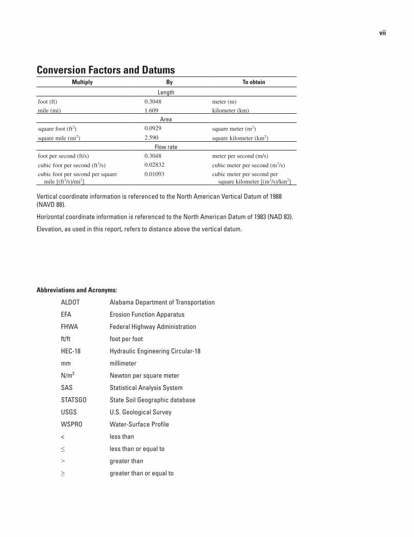
Conversion Factors and DatumsMultiply By To obtain
Lengthfoot (ft) 0.3048 meter (m)
mile (mi) 1.609 kilometer (km)
Areasquare foot (ft2) 0.0929 square meter (m2)
square mile (mi2) 2.590 square kilometer (km2)
Flow ratefoot per second (ft/s) 0.3048 meter per second (m/s)
cubic foot per second (ft3/s) 0.02832 cubic meter per second (m3/s)
cubic foot per second per square mile [(ft3/s)/mi2]
0.01093 cubic meter per second per square kilometer [(m3/s)/km2]
Vertical coordinate information is referenced to the North American Vertical Datum of 1988 (NAVD 88).
Horizontal coordinate information is referenced to the North American Datum of 1983 (NAD 83).
Elevation, as used in this report, refers to distance above the vertical datum.
Abbreviations and Acronyms:
ALDOT Alabama Department of Transportation
EFA Erosion Function Apparatus
FHWA Federal Highway Administration
ft/ft foot per foot
HEC-18 Hydraulic Engineering Circular-18
mm millimeter
N/m2 Newton per square meter
SAS Statistical Analysis System
STATSGO State Soil Geographic database
USGS U.S. Geological Survey
WSPRO Water-Surface Profile
< less than
≤ less than or equal to
> greater than
≥ greater than or equal to

AbstractThe U.S. Geological Survey, in cooperation with the
Alabama Department of Transportation, made observations of clear-water contraction scour at 25 bridge sites in the Black Prairie Belt of the Coastal Plain of Alabama. These bridge sites consisted of 54 hydraulic structures, of which 37 have measurable scour holes. Observed scour depths ranged from 1.4 to 10.4 feet. Theoretical clear-water contraction-scour depths were computed for each bridge and compared with observed scour. This comparison showed that theoretical scour depths, in general, exceeded the observed scour depths by about 475 percent. Variables determined to be important in developing scour in laboratory studies along with several other hydraulic variables were investigated to understand their influence within the Alabama field data. The strongest explanatory variables for clear-water contraction scour were channel-contraction ratio and velocity index. Envelope curves were developed relating both of these explanatory variables to observed scour. These envelope curves provide useful tools for assessing reasonable ranges of scour depth in the Black Prairie Belt of Alabama.
Introduction During 2005, the Nation’s roads experienced an all-time
high in vehicle miles traveled. The U.S. Department of Transportation, Federal Highway Administration (FHWA) documented 3 trillion vehicle miles of travel. A vital part of the road system is safe and functional bridges. Statistics show that 28 percent of the Nation’s highways are considered deficient (Road Information Program, 2002).
Safety of the Nation’s bridges became a major concern in the late 1960s when the structural failure of the Silver Bridge, connecting U.S. Highway 35 over the Ohio River, fatally injured 46 people (National Transportation Safety Board, 1971). Following this event, an amendment was added to the Federal Highway Act of 1968 that required the establishment of the National Bridge Inspection Program. This program was later expanded to investigate failure due to scour after
the collapse of two major bridges occurred during 1987 and 1989. The failure of the Schoharie Creek Bridge in New York State and the Hatchie River Bridge in Tennessee claimed 18 lives (National Transportation Safety Board, 1988; 1990). On recommendation of the National Transportation Safety Board, the FHWA initiated a national program during 1988 to assess the susceptibility of existing and future bridges to scour. This assessment includes the computation of theoretical scour depths, monitoring channel migration, and countermeasures to prevent bridge failure due to scour. In earlier years, the proper research and analytical tools necessary to compute theoretical scour were not available. To address the issue, the FHWA published Hydraulic Engineering Circulars (HEC)-18 and -20 (Richardson and others, 1991; Lagasse and others, 1991). Hydraulic Engineering Circular-18 provides theoretical equations for predicting contraction-scour and local scour depths. Each state was mandated to do qualitative (level 1) and quantitative (level 2) analyses, using these equations. Since 1995, there has been a decrease in the percent of deficient bridges (Road Information Program, 2002). This decrease may be attributed to better inspection policies, technological advances in materials, and more stringent design guidelines.
Forty-eight percent of the Nation’s bridges were built during the period from 1950–1980 (Road Information Program, 2002). As a result, a large number of existing bridges are getting close to the end of their life span. In order to find the most cost-effective methods for replacement or repair of these bridges, current techniques are being reevaluated for more efficient methods. At this time, new bridge construction and countermeasures for existing bridges are designed on the basis of the theoretical scour equations presented in HEC-18. Research has indicated that these equations often provide conservative estimates of scour and in some instances severely overpredict scour depths (Norman, 1975; Holnbeck and others, 1993; Brabets, 1995; Fischer, 1995). Mueller and Wagner (2005) provided a comparison of published literature and field data. Their findings suggest that the accuracy of the contraction-scour equations greatly depends on the degree of contraction, flow distribution, configuration of the approach, and how well the hydraulic model represents the true flow distribution (Mueller and Wagner, 2005).
Clear-Water Contraction Scour at Selected Bridge Sites in the Black Prairie Belt of the Coastal Plain in Alabama, 2006
By K.G. Lee and T.S. Hedgecock
2 Clear-Water Contraction Scour at Selected Bridge Sites in the Black Prairie Belt of the Coastal Plain in Alabama, 2006
Alabama is among many states that have substantial roadway construction needs and limited funding. According to statistics published during 2005, Alabama’s road system accommodated about 59 billion vehicle miles of travel (U.S. Department of Transportation Federal Highway Administra-tion, 2006), and the census has projected a steady increase in Alabama’s population, which will likely result in greater road traffic. With increases in traffic, there is a high demand for bridges to be functional and safe. Many of Alabama’s bridges are approaching the end of their 50-year expected life span. About $50 million is spent annually for repair and replacement of bridges in the State of Alabama (Government Performance Project, 2005).
To address the concern of economic feasibility of new bridge construction and countermeasures for existing structures, alternative methods for computing theoretical scour depths have been explored in other states. Methods of relating hydraulic properties to measured scour depths are outlined by Benedict (2003) in Clear-Water Abutment and Contrac-tion Scour in the Coastal Plain and Piedmont Provinces of South Carolina, 1996–99. That study and a following study (Benedict and Caldwell, 2005) were successful in developing correlations that are useful in the assessment of clear-water scour.
The U.S. Geological Survey (USGS), in cooperation with the Alabama Department of Transportation (ALDOT), initiated a study, using a similar approach, to investigate alternative methods for computing clear-water contraction-scour depths in the cohesive soils located in the Black Prairie Belt of the Coastal Plain of Alabama (fig. 1).
Purpose and Scope
This report describes (1) techniques used to collect clear-water contraction scour data at 25 bridge sites (37 hydraulic structures) in the Black Prairie Belt of the Coastal Plain of Alabama, (2) a comparison of theoretical clear-water contraction-scour depths with observed scour depths, (3) selected relations within the field data, (4) envelope curves that may be used to estimate ranges of anticipated clear-water contraction scour for bridges in the Black Prairie Belt of the Coastal Plain of Alabama, and (5) pier-scour observations and insights for bridges in the Black Prairie Belt of the Coastal Plain of Alabama.
Acknowledgments
The assistance of Mr. Tom Flournoy, ALDOT Bridge Hydraulics Engineer, and Mr. Eric Christy, ALDOT Assistant State Maintenance Engineer, is greatly appreciated. The Testing Division of the ALDOT Bureau of Materials and Test also was instrumental in providing grain-size distribution analyses for all of the sites included in this study. Also, special thanks are given to Mr. Benjamin Dewit and Miss Britane
Bell, engineering students at Auburn University, for their contributions to this study.
Description of Study Area
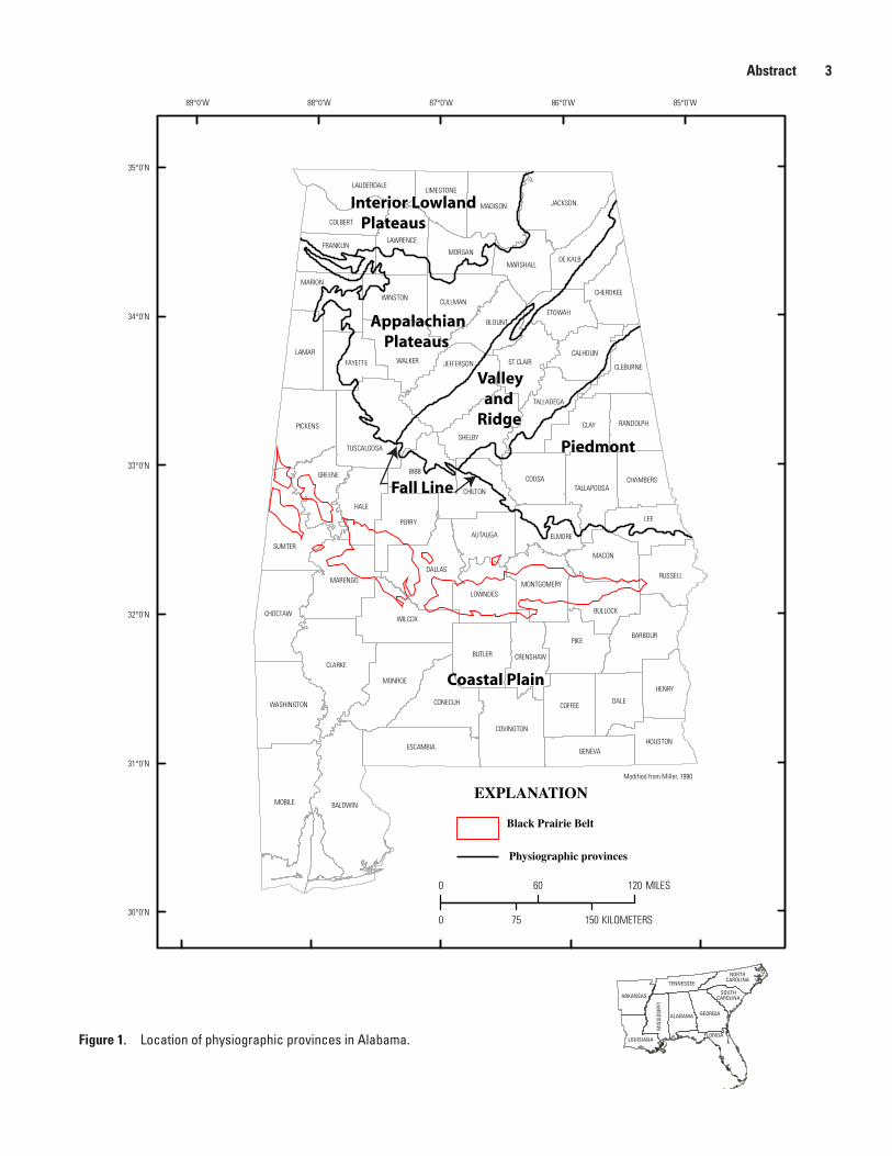
The physiography of Alabama is divided into five regions: Coastal Plain, Appalachian Plateaus, Piedmont, Valley and Ridge, and Interior Lowland Plateaus (fig. 1). The largest physiographic region in Alabama is the Coastal Plain. The Coastal Plain covers about 59 percent of the State’s 51,600 square miles (mi2) of area. This region is subdivided into four subregions called districts. Based on previous unpublished scour assessments, the Black Prairie Belt district, located in the upper half of the Coastal Plain, was determined to be the area of greatest concern for accurate bridge-scour determinations.
The Black Prairie Belt extends from Russell County, Alabama, through east-central Mississippi and thins out north of the Tennessee State line. A prairie is defined as a large area of undulating valley covered by coarse grasses and minimal trees. The Black Prairie Belt is composed of sedimentary soils of Cretaceous age. In this area, Selma chalk is overlain with rich black soil that is characterized as consolidated and highly cohesive clay that contains significant amounts of organic matter (Fenneman, 1938).
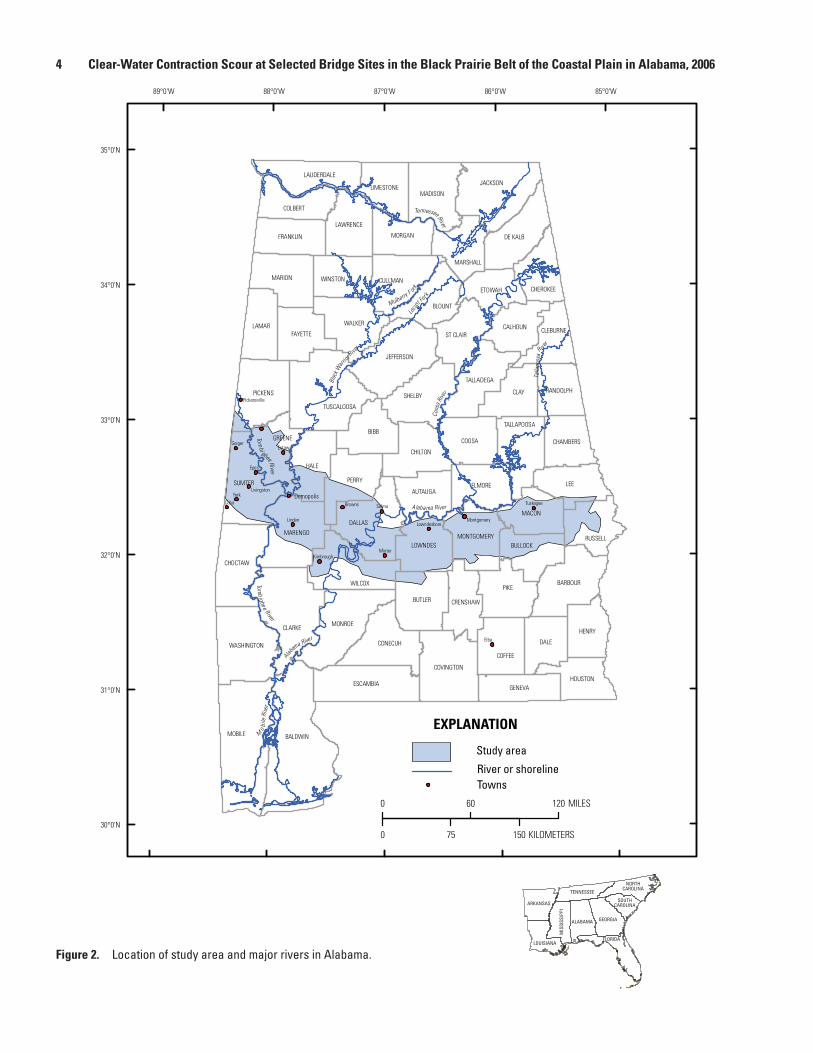
The crescent-shaped Black Prairie Belt occupies about 4,300 mi2 in Alabama, ranging from 35 to 46 miles (mi) in width (Rankin, 1974). The Black Prairie Belt extends through 13 counties in Alabama: Bullock, Dallas, Greene, Hale, Lowndes, Macon, Marengo, Montgomery, Perry, Pickens, Russell, Sumter, and Wilcox. The major streams in Alabama’s portion of the Black Prairie Belt are the Black Warrior, Alabama, and Tombigbee Rivers (Fenneman, 1938). The Tombigbee River flows southeastward and joins the Black Warrior at Demopolis and turns in a southwestward direction as it flows through the western portion of the Black Prairie Belt. The confluence of the Coosa and Tallapoosa Rivers form the Alabama River (fig. 2). The elevation between streams in some areas is minimal and provides little topographic relief. The Black Prairie Belt is often described as a peneplain, indicating relief has been shaped through erosion. The average elevation of Alabama’s portion of the Black Prairie Belt is 225 feet (ft) (U.S. Geological Survey, 2006).
The study area was determined by compiling several maps. Depending on the source, date, and detail of the map, the extent of the Black Prairie Belt boundary varies. To determine the most extensive study area, general soils maps were compared with the physiographic provinces. These maps were overlain with the State Soil Geographic (STATSGO) database. The STATSGO database is a generalization of a detailed soil survey that provides a representation of soil patterns in a landscape (National Resource Conservation Service, 2006). The soil patterns of the Black Prairie Belt were selected, and the study area was defined. The resulting study area (fig. 2) was determined to be 6,150 mi2 in area and
Abstract 3
Figure 1. Location of physiographic provinces in Alabama.
LEE
BALDWINMOBILE
CLARKE
PIKE
BIBB
HALE
DALLAS
CLAY
JACKSON
PERRY
WILCOX
MONROE
DALE
SUMTER
SHELBY
PICKENS
BUTLER
TUSCALOOSA
JEFFERSONWALKER
COFFEE
COOSA
BARBOUR
DE KALB
MARENGO
CHOCTAW
ESCAMBIA
MARION
COVINGTON
CONECUH
GREENE
CHILTON
LAMAR
HENRY
MADISON
BLOUNT
ELMORE
MACON
WASHINGTON
FAYETTE
CULLMAN
RUSSELL
ST CLAIR
GENEVA
COLBERT
LOWNDES
BULLOCK
TALLADEGA
FRANKLINLAWRENCE
MORGAN
WINSTON
CALHOUN
ETOWAH
AUTAUGA
TALLAPOOSA
HOUSTON
CHEROKEE
MARSHALL
LAUDERDALE
CLEBURNE
RANDOLPH
MONTGOMERY
CHAMBERS
LIMESTONE
CRENSHAW
89°0'W 88°0'W 87°0'W 86°0'W 85°0'W
30°0'N
31°0'N
32°0'N
33°0'N
34°0'N
35°0'N
0 75 150 KILOMETERS
0 60 120 MILES
EXPLANATION
Black Prairie Belt
Physiographic provinces
Interior Lowland Plateaus
Appalachian Plateaus
Valley and Ridge
Piedmont
Coastal Plain
Fall Line
Modified from Miller, 1990
NORTHCAROLINA
SOUTHCAROLINA
GEORGIAALABAMA
LOUISIANA
ARKANSAS
TENNESSEE
MIS
SISS
IPPI
FLORIDA
NORTHCAROLINA
SOUTHCAROLINA
GEORGIAALABAMA
LOUISIANA
ARKANSAS
TENNESSEE
MIS
SISS
IPPI
FLORIDA
4 Clear-Water Contraction Scour at Selected Bridge Sites in the Black Prairie Belt of the Coastal Plain in Alabama, 2006
Figure 2. Location of study area and major rivers in Alabama.
Mo
bile
Rive
r
Alabama River
Tomb
igbee River
Alaba ma River
Coos
a Rive
r
MulberryF ork
Tennessee River
Tombi gbeeRiver
Demopolis
Blac
k Warr
iorRive
r
Locu
stFor k
LEE
BALDWINMOBILE
CLARKE
PIKE
BIBB
HALE
DALLAS
CLAY
JACKSON
PERRY
WILCOX
MONROE
DALE
SUMTER
SHELBYPICKENS
BUTLER
TUSCALOOSA
JEFFERSON
WALKER
COFFEE
COOSA
BARBOUR
DE KALB
MARENGO
CHOCTAW
ESCAMBIA
MARION
COVINGTON
CONECUH
GREENE
CHILTON
LAMAR
HENRY
MADISON
BLOUNT
ELMORE
MACON
WASHINGTON
FAYETTE
CULLMAN
RUSSELL
ST CLAIR
GENEVA
COLBERT
LOWNDES BULLOCK
TALLADEGA
FRANKLIN
LAWRENCE
MORGAN
WINSTON
CALHOUN
ETOWAH
AUTAUGA
TALLAPOOSA
HOUSTON
CHEROKEE
MARSHALL
LAUDERDALE
CLEBURNE
RANDOLPH
MONTGOMERY
CHAMBERS
LIMESTONE
CRENSHAW
York
Epes
Elba
Cuba
Eutaw
SelmaBrowns
Minter
Linden
Geiger
Tuskegee
Kimbrough
Livingston
MontgomeryLowndesboro
Pickensville
89°0'W 88°0'W 87°0'W 86°0'W 85°0'W
30°0'N
31°0'N
32°0'N
33°0'N
34°0'N
35°0'N
0 75 150 KILOMETERS
0 60 120 MILES
EXPLANATION
Study area
River or shorelineTowns
Talla
poos
aR ive
r
NORTHCAROLINA
SOUTHCAROLINA
GEORGIAALABAMA
LOUISIANA
ARKANSAS
TENNESSEE
MIS
SISS
IPPI
FLORIDA
NORTHCAROLINA
SOUTHCAROLINA
GEORGIAALABAMA
LOUISIANA
ARKANSAS
TENNESSEE
MIS
SISS
IPPI
FLORIDA
Abstract 5
The bridge sites were visited and the current field conditions documented. A detailed summary of each bridge included measurement of the existing hydraulic structure, verification of previous floodplain surveys, measurement of high-water marks, selection of Manning’s roughness coef-ficients, and observations of land use in the drainage basin. These measurements and observations were notated and used in hydrologic and hydraulic computations.
Other field data measurements included depth of existing scour holes and estimates of soil classification. The properties computed from the hydraulic model and the soil classification were used as input variables in the theoretical scour equations presented in HEC-18. Contraction and local scour were computed for the 100- and 500-year recurrence interval flood discharges, unless significant roadway overtopping occurred. In the case of roadway overtopping, the recurrence interval
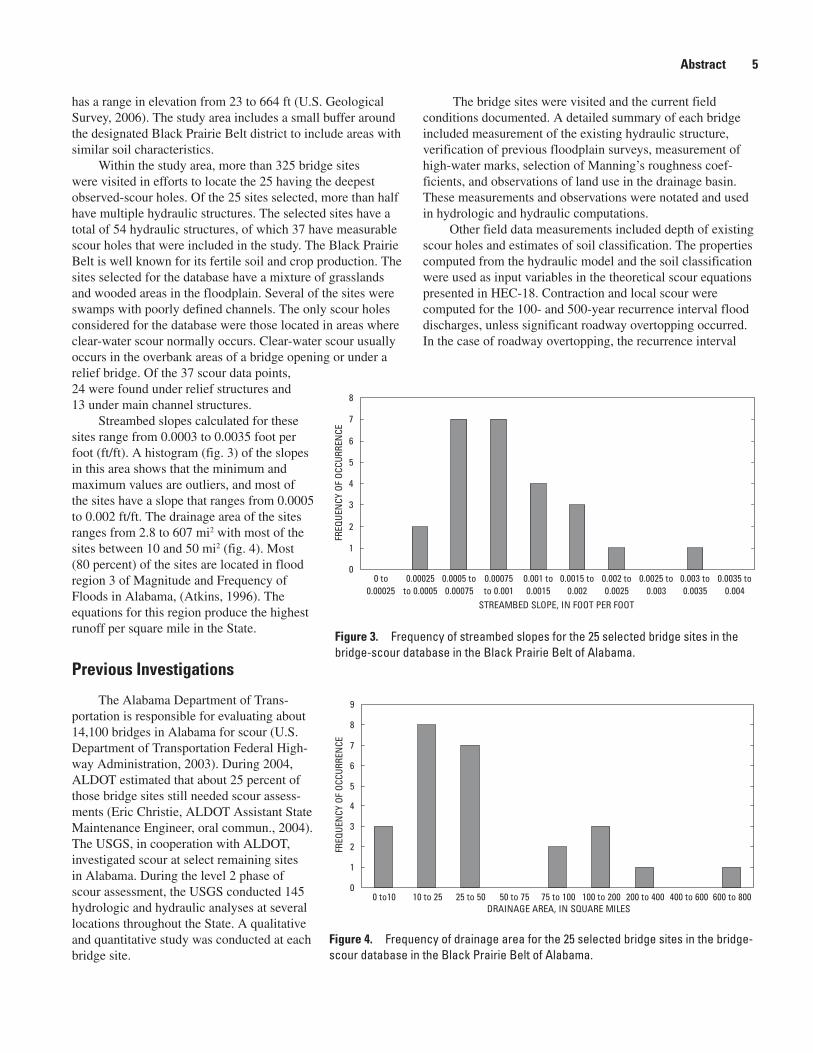
Figure 3. Frequency of streambed slopes for the 25 selected bridge sites in the bridge-scour database in the Black Prairie Belt of Alabama.
has a range in elevation from 23 to 664 ft (U.S. Geological Survey, 2006). The study area includes a small buffer around the designated Black Prairie Belt district to include areas with similar soil characteristics.
Within the study area, more than 325 bridge sites were visited in efforts to locate the 25 having the deepest observed-scour holes. Of the 25 sites selected, more than half have multiple hydraulic structures. The selected sites have a total of 54 hydraulic structures, of which 37 have measurable scour holes that were included in the study. The Black Prairie Belt is well known for its fertile soil and crop production. The sites selected for the database have a mixture of grasslands and wooded areas in the floodplain. Several of the sites were swamps with poorly defined channels. The only scour holes considered for the database were those located in areas where clear-water scour normally occurs. Clear-water scour usually occurs in the overbank areas of a bridge opening or under a relief bridge. Of the 37 scour data points, 24 were found under relief structures and 13 under main channel structures.
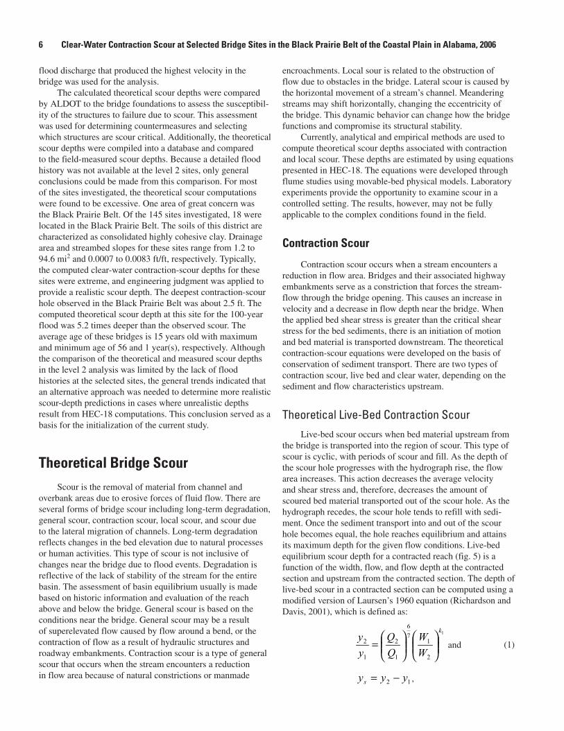
Streambed slopes calculated for these sites range from 0.0003 to 0.0035 foot per foot (ft/ft). A histogram (fig. 3) of the slopes in this area shows that the minimum and maximum values are outliers, and most of the sites have a slope that ranges from 0.0005 to 0.002 ft/ft. The drainage area of the sites ranges from 2.8 to 607 mi2 with most of the sites between 10 and 50 mi2 (fig. 4). Most (80 percent) of the sites are located in flood region 3 of Magnitude and Frequency of Floods in Alabama, (Atkins, 1996). The equations for this region produce the highest runoff per square mile in the State.
Previous Investigations
The Alabama Department of Trans-portation is responsible for evaluating about 14,100 bridges in Alabama for scour (U.S. Department of Transportation Federal High-way Administration, 2003). During 2004, ALDOT estimated that about 25 percent of those bridge sites still needed scour assess-ments (Eric Christie, ALDOT Assistant State Maintenance Engineer, oral commun., 2004). The USGS, in cooperation with ALDOT, investigated scour at select remaining sites in Alabama. During the level 2 phase of scour assessment, the USGS conducted 145 hydrologic and hydraulic analyses at several locations throughout the State. A qualitative and quantitative study was conducted at each bridge site.
Figure 4. Frequency of drainage area for the 25 selected bridge sites in the bridge-scour database in the Black Prairie Belt of Alabama.
0
1
2
3
4
5
6
7
8
0 to0.00025
0.00025to 0.0005
0.0005 to0.00075
0.00075to 0.001
0.001 to0.0015
0.0015 to0.002
0.002 to0.0025
0.0025 to0.003
0.003 to0.0035
0.0035 to0.004
STREAMBED SLOPE, IN FOOT PER FOOT
FREQ
UEN
CY O
F OC
CURR
ENCE
0
1
2
3
4
5
6
7
8
9
0 to10 10 to 25 25 to 50 50 to 75 75 to 100 100 to 200 200 to 400 400 to 600 600 to 800DRAINAGE AREA, IN SQUARE MILES
FREQ
UEN
CY O
F OC
CURR
ENCE
6 Clear-Water Contraction Scour at Selected Bridge Sites in the Black Prairie Belt of the Coastal Plain in Alabama, 2006
flood discharge that produced the highest velocity in the bridge was used for the analysis.
The calculated theoretical scour depths were compared by ALDOT to the bridge foundations to assess the susceptibil-ity of the structures to failure due to scour. This assessment was used for determining countermeasures and selecting which structures are scour critical. Additionally, the theoretical scour depths were compiled into a database and compared to the field-measured scour depths. Because a detailed flood history was not available at the level 2 sites, only general conclusions could be made from this comparison. For most of the sites investigated, the theoretical scour computations were found to be excessive. One area of great concern was the Black Prairie Belt. Of the 145 sites investigated, 18 were located in the Black Prairie Belt. The soils of this district are characterized as consolidated highly cohesive clay. Drainage area and streambed slopes for these sites range from 1.2 to 94.6 mi2 and 0.0007 to 0.0083 ft/ft, respectively. Typically, the computed clear-water contraction-scour depths for these sites were extreme, and engineering judgment was applied to provide a realistic scour depth. The deepest contraction-scour hole observed in the Black Prairie Belt was about 2.5 ft. The computed theoretical scour depth at this site for the 100-year flood was 5.2 times deeper than the observed scour. The average age of these bridges is 15 years old with maximum and minimum age of 56 and 1 year(s), respectively. Although the comparison of the theoretical and measured scour depths in the level 2 analysis was limited by the lack of flood histories at the selected sites, the general trends indicated that an alternative approach was needed to determine more realistic scour-depth predictions in cases where unrealistic depths result from HEC-18 computations. This conclusion served as a basis for the initialization of the current study.
Theoretical Bridge Scour Scour is the removal of material from channel and
overbank areas due to erosive forces of fluid flow. There are several forms of bridge scour including long-term degradation, general scour, contraction scour, local scour, and scour due to the lateral migration of channels. Long-term degradation reflects changes in the bed elevation due to natural processes or human activities. This type of scour is not inclusive of changes near the bridge due to flood events. Degradation is reflective of the lack of stability of the stream for the entire basin. The assessment of basin equilibrium usually is made based on historic information and evaluation of the reach above and below the bridge. General scour is based on the conditions near the bridge. General scour may be a result of superelevated flow caused by flow around a bend, or the contraction of flow as a result of hydraulic structures and roadway embankments. Contraction scour is a type of general scour that occurs when the stream encounters a reduction in flow area because of natural constrictions or manmade
encroachments. Local sour is related to the obstruction of flow due to obstacles in the bridge. Lateral scour is caused by the horizontal movement of a stream’s channel. Meandering streams may shift horizontally, changing the eccentricity of the bridge. This dynamic behavior can change how the bridge functions and compromise its structural stability.
Currently, analytical and empirical methods are used to compute theoretical scour depths associated with contraction and local scour. These depths are estimated by using equations presented in HEC-18. The equations were developed through flume studies using movable-bed physical models. Laboratory experiments provide the opportunity to examine scour in a controlled setting. The results, however, may not be fully applicable to the complex conditions found in the field.
Contraction Scour
Contraction scour occurs when a stream encounters a reduction in flow area. Bridges and their associated highway embankments serve as a constriction that forces the stream-flow through the bridge opening. This causes an increase in velocity and a decrease in flow depth near the bridge. When the applied bed shear stress is greater than the critical shear stress for the bed sediments, there is an initiation of motion and bed material is transported downstream. The theoretical contraction-scour equations were developed on the basis of conservation of sediment transport. There are two types of contraction scour, live bed and clear water, depending on the sediment and flow characteristics upstream.
Theoretical Live-Bed Contraction ScourLive-bed scour occurs when bed material upstream from
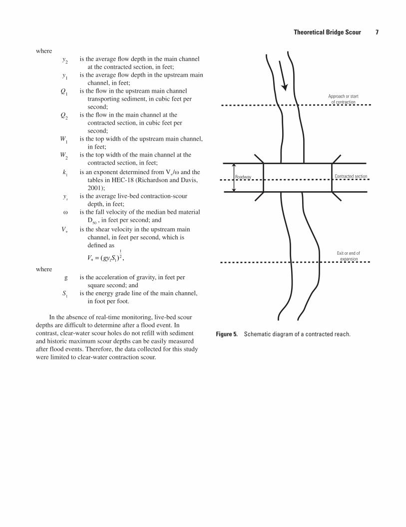
the bridge is transported into the region of scour. This type of scour is cyclic, with periods of scour and fill. As the depth of the scour hole progresses with the hydrograph rise, the flow area increases. This action decreases the average velocity and shear stress and, therefore, decreases the amount of scoured bed material transported out of the scour hole. As the hydrograph recedes, the scour hole tends to refill with sedi-ment. Once the sediment transport into and out of the scour hole becomes equal, the hole reaches equilibrium and attains its maximum depth for the given flow conditions. Live-bed equilibrium scour depth for a contracted reach (fig. 5) is a function of the width, flow, and flow depth at the contracted section and upstream from the contracted section. The depth of live-bed scour in a contracted section can be computed using a modified version of Laursen’s 1960 equation (Richardson and Davis, 2001), which is defined as:
1
2
176
1
2
1
2
k
WW
yy
= and
12 yyys −=
(1)
,
Theoretical Bridge Scour 7
where y
2 is the average flow depth in the main channel
at the contracted section, in feet; y
1 is the average flow depth in the upstream main
channel, in feet; Q
1 is the flow in the upstream main channel
transporting sediment, in cubic feet per second;
Q2
is the flow in the main channel at the contracted section, in cubic feet per second;
W1
is the top width of the upstream main channel, in feet;
W2 is the top width of the main channel at the
contracted section, in feet;
k1 is an exponent determined from V
*/ω and the
tables in HEC-18 (Richardson and Davis, 2001);
ys is the average live-bed contraction-scour
depth, in feet; ω is the fall velocity of the median bed material
D50
, in feet per second; and
V* is the shear velocity in the upstream main
channel, in feet per second, which is defined as
where g is the acceleration of gravity, in feet per
square second; and S
1 is the energy grade line of the main channel,
in foot per foot.
In the absence of real-time monitoring, live-bed scour depths are difficult to determine after a flood event. In contrast, clear-water scour holes do not refill with sediment and historic maximum scour depths can be easily measured after flood events. Therefore, the data collected for this study were limited to clear-water contraction scour.
Figure 5. Schematic diagram of a contracted reach.
12
1 1( ) ,V gy S∗ =
Roadway
Approach or start of contraction
Exit or end of expansion
Contracted section
8 Clear-Water Contraction Scour at Selected Bridge Sites in the Black Prairie Belt of the Coastal Plain in Alabama, 2006
Theoretical Clear-Water Contraction Scour
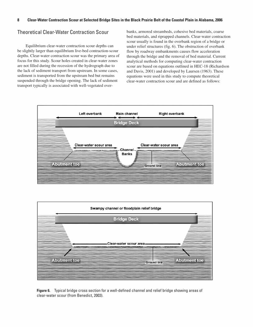
Equilibrium clear-water contraction scour depths can be slightly larger than equilibrium live-bed contraction-scour depths. Clear-water contraction scour was the primary area of focus for this study. Scour holes created in clear-water zones are not filled during the recession of the hydrograph due to the lack of sediment transport from upstream. In some cases, sediment is transported from the upstream bed but remains suspended through the bridge opening. The lack of sediment transport typically is associated with well-vegetated over-
banks, armored streambeds, cohesive bed materials, coarse bed materials, and riprapped channels. Clear-water contraction scour usually is found in the overbank region of a bridge or under relief structures (fig. 6). The obstruction of overbank flow by roadway embankments causes flow acceleration through the bridge and the removal of bed material. Current analytical methods for computing clear-water contraction scour are based on equations outlined in HEC-18 (Richardson and Davis, 2001) and developed by Laursen (1963). These equations were used in this study to compute theoretical clear-water contraction scour and are defined as follows:
Figure 6. Typical bridge cross section for a well-defined channel and relief bridge showing areas of clear-water scour (from Benedict, 2003).
Site Selection 9
and (2)
where y
2 is the average equilibrium flow depth in the
contracted section after the contraction scour, in feet;
Q is the discharge through the bridge or on the set-back overbank area at the bridge associated with the width W, in cubic feet per second;
Dm
is the diameter of the smallest nontransportable particle in the bed material in the contracted section, in feet, and is defined as ;
D50
is the median diameter of bed material, in feet;
W is the width of the contracted section less pier widths, in feet;
ys is the average scour depth in the contracted
section, in feet; y
1 is the average depth of flow in the contracted
section prior to contraction scour, in feet; and
Ku is a constant value of 0.0077 for English units.
Pier Scour
Pier scour is a result of flow obstruction within the bridge, associated with the bridge piers. The obstruction of flow changes the natural streamlines and causes the formation of vortices. Theses vortices are referred to as horseshoe vortices and wake vortices. As water stacks up and is acceler-ated around the upstream face of the pier, a horseshoe vortex is formed. This downward acceleration results in the removal of bed material around the pier. Wake vortices act in the vertical direction and are formed downstream from the pier. Both types of vortices contribute to the removal of bed material and the deepening of the scour hole. The depth of the hole continues to increase until equilibrium is reached. In the case of live-bed pier scour, equilibrium conditions are achieved when sediment transport into and out of the scour hole is balanced. In the case of clear-water pier scour, scouring continues until the stress resulting from the vortices is no longer great enough to exceed the critical shear stress of the sediment. Theoretical pier-scour depth can be calculated using the following equation sug-gested in HEC-18 (Richardson and Davis, 2001).
where y
s is the theoretical pier-scour depth, in feet;
a is the pier width, in feet; K
1 is the dimensionless correction factor for pier
nose shape; K
2 is the dimensionless correction factor for
angle of attack for flow; K
3 is the dimensionless correction factor for bed
condition; K
4 is the dimensionless correction factor for bed
armoring; y
1 is the approach flow depth, in feet; and
Fr1 is the Froude number directly upstream from
the pier and defined as
where V
1 is the mean velocity directly upstream from
the pier, in feet per second; and g is the acceleration of gravity, in feet per
square second.
Site Selection The study area (fig. 2) was used as the basis for selecting
sites for field reconnaissance. The sites selected for investiga-tion are stream crossings having older, multiple-span bridges with the potential for scour holes. Crossings with culverts, single-span bridges, and bridges over major rivers were eliminated. A total of 325 sites were investigated for use in the scour database. Of the 325 sites, 16 were railroad structures. The only railroad structures considered for the database were those constructed similar to highway structures.
Each site was investigated for the presence of scour holes, and the age and condition of the structure were documented. A field dilatancy test was performed on the soil near the bridge to determine if the soil was primarily clay or silt. A list was compiled of the sites that had significant scour holes and showed characteristics of the soils indicative of the Black Prairie Belt.
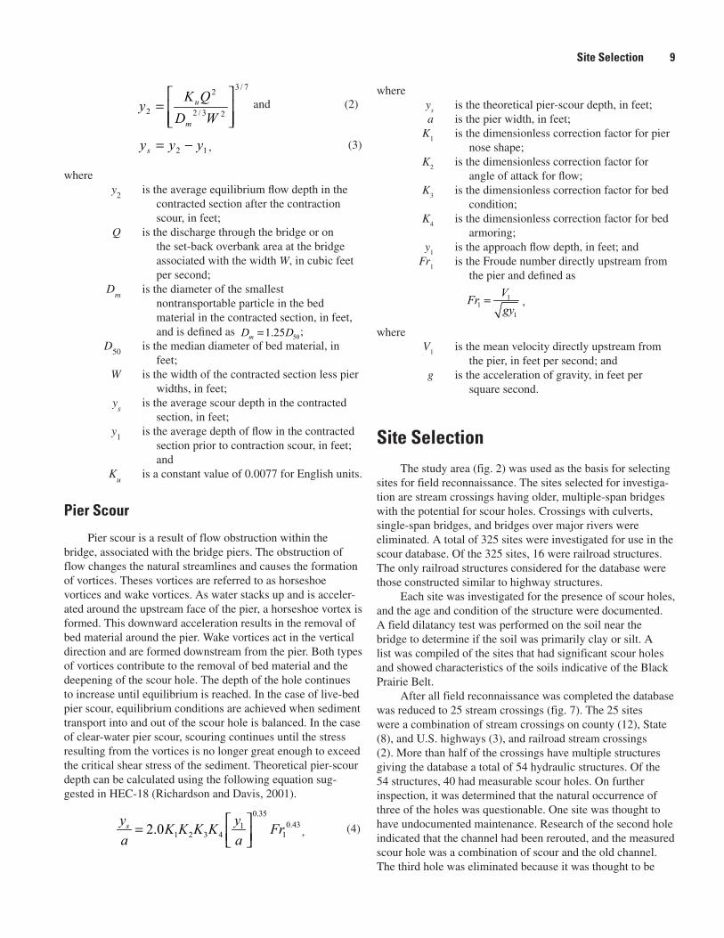
After all field reconnaissance was completed the database was reduced to 25 stream crossings (fig. 7). The 25 sites were a combination of stream crossings on county (12), State (8), and U.S. highways (3), and railroad stream crossings (2). More than half of the crossings have multiple structures giving the database a total of 54 hydraulic structures. Of the 54 structures, 40 had measurable scour holes. On further inspection, it was determined that the natural occurrence of three of the holes was questionable. One site was thought to have undocumented maintenance. Research of the second hole indicated that the channel had been rerouted, and the measured scour hole was a combination of scour and the old channel. The third hole was eliminated because it was thought to be
7/3
23/2
2
2
=
WDQK
ym
u
12 yyys −= (3)
501.25mD D=
(4)0.35
0.4311 2 3 4 12.0sy yK K K K Fr
a a =
11
1
VFrgy
=
,
,
,
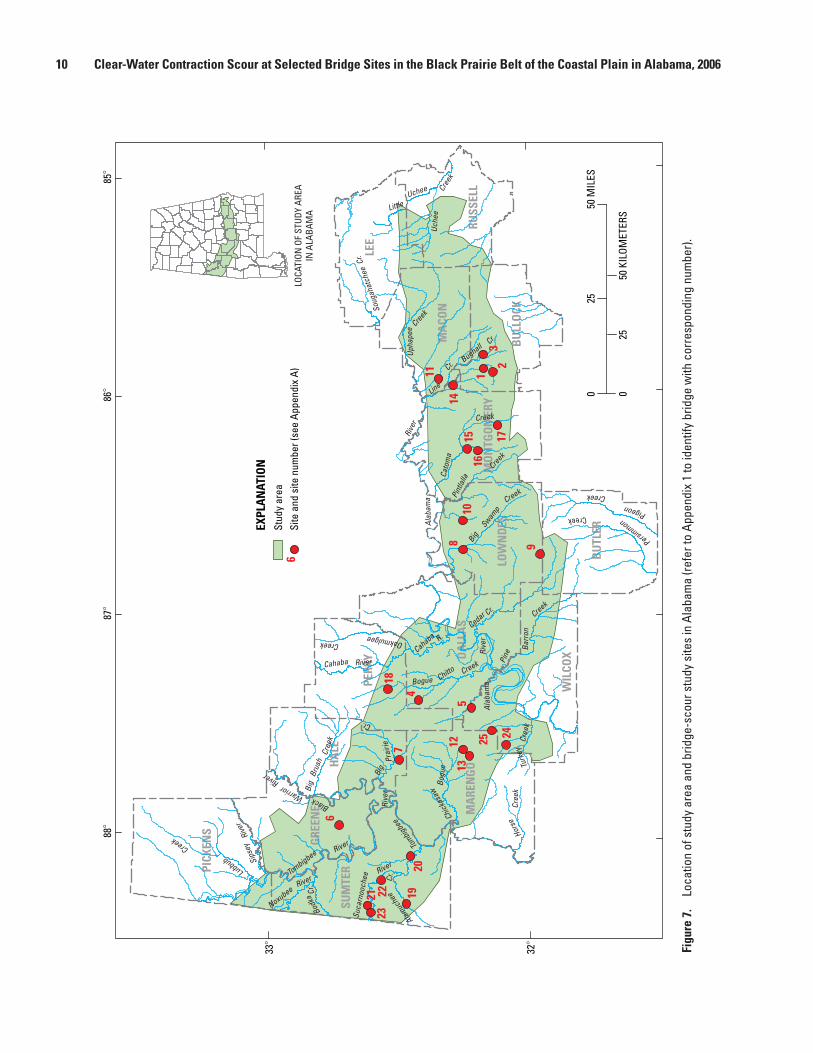
10 Clear-Water Contraction Scour at Selected Bridge Sites in the Black Prairie Belt of the Coastal Plain in Alabama, 2006
Figu
re 7
. Lo
catio
n of
stu
dy a
rea
and
brid
ge-s
cour
stu
dy s
ites
in A
laba
ma
(refe
r to
Appe
ndix
1 to
iden
tify
brid
ge w
ith c
orre
spon
ding
num
ber).
HA
LE
PERR
Y DA
LLA
S
LOW
ND
ESM
ON
TGO
MER
Y
BU
TLER
LEE
RUSS
ELL
WIL
COX
MA
CON
BU
LLO
CK
MA
REN
GO
GRE
ENE
PICK
ENS
SUM
TER
EXPL
AN
ATIO
NSt
udy
area
Site
and
site
num
ber (
see
Appe
ndix
A)
LOCA
TION
OF
STUD
Y AR
EAIN
ALA
BAM
A
6
21
20
22 19
237
18
4
1312
5
25 24
9810
1615 17
2
14
3
11 1
6
Soug
ahat
chee
Cr.
Uche
e
Uchee
Little
Cree
k
Upha
pee
Cr.
Creek
Line
Bughall Cr.
Creek
Cato
ma
Pint
lalla
BigSwam
p
Alab
ama
Rive
r
CreekCreek
Alab
ama
Rive
r
Cedar Cr.
Cahaba
Bogue Chitto Creek
R.
Cahaba River Pine
Barr
on
Creek
Turk
eyCr
eek
Hors
eChick
asaw
Cr.
Cree
k
Bogu
e
Big
Big
Brus
h Prai
rie
Tombig
bee
Alamuc
hee
Rive
rCr
.
Suca
rnoo
chee
River
River
Bodk
a
Lubbub
Noxubee
Tombigbee
Cr.River
Creek
Sips
eyBlackWarrio
r
Rive
r
River
Cree
k
OakmulgeeCreek
PersimmonPigeon
Creek
Creek
025
50 K
ILOM
ETER
S
025
50 M
ILES
88
87
86
85
33
32
Data Assumptions 11
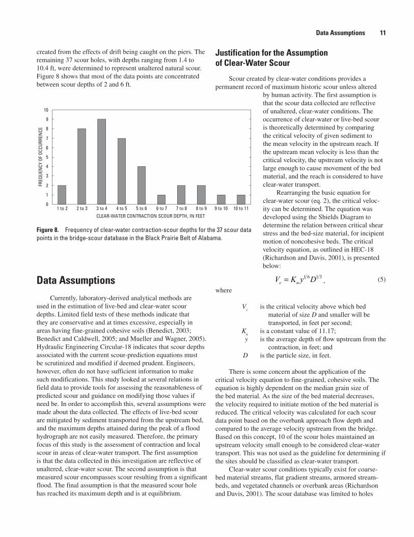
created from the effects of drift being caught on the piers. The remaining 37 scour holes, with depths ranging from 1.4 to 10.4 ft, were determined to represent unaltered natural scour. Figure 8 shows that most of the data points are concentrated between scour depths of 2 and 6 ft.
Justification for the Assumption of Clear-Water Scour
Scour created by clear-water conditions provides a permanent record of maximum historic scour unless altered
by human activity. The first assumption is that the scour data collected are reflective of unaltered, clear-water conditions. The occurrence of clear-water or live-bed scour is theoretically determined by comparing the critical velocity of given sediment to the mean velocity in the upstream reach. If the upstream mean velocity is less than the critical velocity, the upstream velocity is not large enough to cause movement of the bed material, and the reach is considered to have clear-water transport.
Rearranging the basic equation for clear-water scour (eq. 2), the critical veloc-ity can be determined. The equation was developed using the Shields Diagram to determine the relation between critical shear stress and the bed-size material, for incipient motion of noncohesive beds. The critical
velocity equation, as outlined in HEC-18 (Richardson and Davis, 2001), is presented below:
where
Vc is the critical velocity above which bed
material of size D and smaller will be transported, in feet per second;
Ku is a constant value of 11.17;
y is the average depth of flow upstream from the contraction, in feet; and
D is the particle size, in feet.
There is some concern about the application of the critical velocity equation to fine-grained, cohesive soils. The equation is highly dependent on the median grain size of the bed material. As the size of the bed material decreases, the velocity required to initiate motion of the bed material is reduced. The critical velocity was calculated for each scour data point based on the overbank approach flow depth and compared to the average velocity upstream from the bridge. Based on this concept, 10 of the scour holes maintained an upstream velocity small enough to be considered clear-water transport. This was not used as the guideline for determining if the sites should be classified as clear-water transport.
Clear-water scour conditions typically exist for coarse-bed material streams, flat gradient streams, armored stream-beds, and vegetated channels or overbank areas (Richardson and Davis, 2001). The scour database was limited to holes
Figure 8. Frequency of clear-water contraction-scour depths for the 37 scour data points in the bridge-scour database in the Black Prairie Belt of Alabama.
1 6 1 3c uV K y D= (5),Data Assumptions
Currently, laboratory-derived analytical methods are used in the estimation of live-bed and clear-water scour depths. Limited field tests of these methods indicate that they are conservative and at times excessive, especially in areas having fine-grained cohesive soils (Benedict, 2003; Benedict and Caldwell, 2005; and Mueller and Wagner, 2005). Hydraulic Engineering Circular-18 indicates that scour depths associated with the current scour-prediction equations must be scrutinized and modified if deemed prudent. Engineers, however, often do not have sufficient information to make such modifications. This study looked at several relations in field data to provide tools for assessing the reasonableness of predicted scour and guidance on modifying those values if need be. In order to accomplish this, several assumptions were made about the data collected. The effects of live-bed scour are mitigated by sediment transported from the upstream bed, and the maximum depths attained during the peak of a flood hydrograph are not easily measured. Therefore, the primary focus of this study is the assessment of contraction and local scour in areas of clear-water transport. The first assumption is that the data collected in this investigation are reflective of unaltered, clear-water scour. The second assumption is that measured scour encompasses scour resulting from a significant flood. The final assumption is that the measured scour hole has reached its maximum depth and is at equilibrium.
0
1
2
3
4
5
6
7
8
9
10
1 to 2 2 to 3 3 to 4 4 to 5 5 to 6 6 to 7 7 to 8 8 to 9 9 to 10 10 to 11
CLEAR-WATER CONTRACTION SCOUR DEPTH, IN FEET
FREQ
UEN
CY O
F OC
CURR
ENCE
12 Clear-Water Contraction Scour at Selected Bridge Sites in the Black Prairie Belt of the Coastal Plain in Alabama, 2006
located in the overbank regions and under relief structures. The overbank bed material upstream from the bridge is secured by the root systems of vegetation The cohesive nature of the soil at these sites also limits any bed load transport, making clear-water scour conditions a reasonable assumption for these sites even though the computed critical velocity for noncohesive soils suggests otherwise.
Additionally, it is important that scour measured in this study reflects scour unaltered by road maintenance. For all sites located on a county route, the respective county engineer was contacted. A copy was obtained of the maintenance logs, date of construction, and bridge soundings. The date of construction was compared to the applicable flood dates, and the bridge soundings were inspected for any unusual changes in ground elevation. Similar documents were obtained for State and U.S routes in addition to any applicable highway plans. Inspection of these documents indicated that the scour holes existed in their original form and had not been altered. Based on field observations, it was determined that the scour holes present at the railroad structures were unaltered by maintenance. The age of the railroad structures was not directly determined. Based on the condition and lifespan of the structures, it was assumed that they were at least 75 years old or older.
Justification for the Assumption of Large Flood Flows
The scour data points were neither measured during or directly after a flood event. Research was used to confirm that each bridge had experienced a significant flood and to determine the correlation flood associated with the measured scour holes. The correlation flood is defined as the largest probable flood associated with the hydraulics creating the scour hole. The justification of large flood flows was accomplished through the use of gage data, flood reports, and statistical flood risk analysis.
Theoretical scour is based on hydraulic properties reflective of the 100- and 500-year floods, unless significant overtopping occurs. If significant overtopping occurs, the bridge is provided relief and velocities are reduced. When this is the case, the maximum scour is a result of a lesser recurrence interval flood. The ALDOT designs State highway crossings based on the criteria of a 50-year flood and county road crossings on the 25-year flood. It would be a reasonable assumption that most of these roadways are overtopped to a certain degree by the 500-year flood, unless the design of the structure is not governed by hydraulics. Also, the probability
of a bridge experiencing multiple 500-year floods during its life span is low. Therefore, for this study, a significant flood is defined as a 50- to 100-year flood event. Documentation of significant flooding and determination of the correlation flood was accomplished through the use of historical floods and statistical risk analyses.
Historical Floods
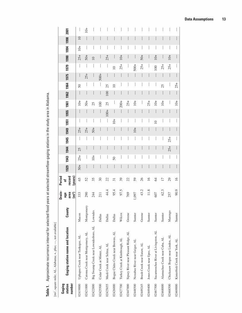
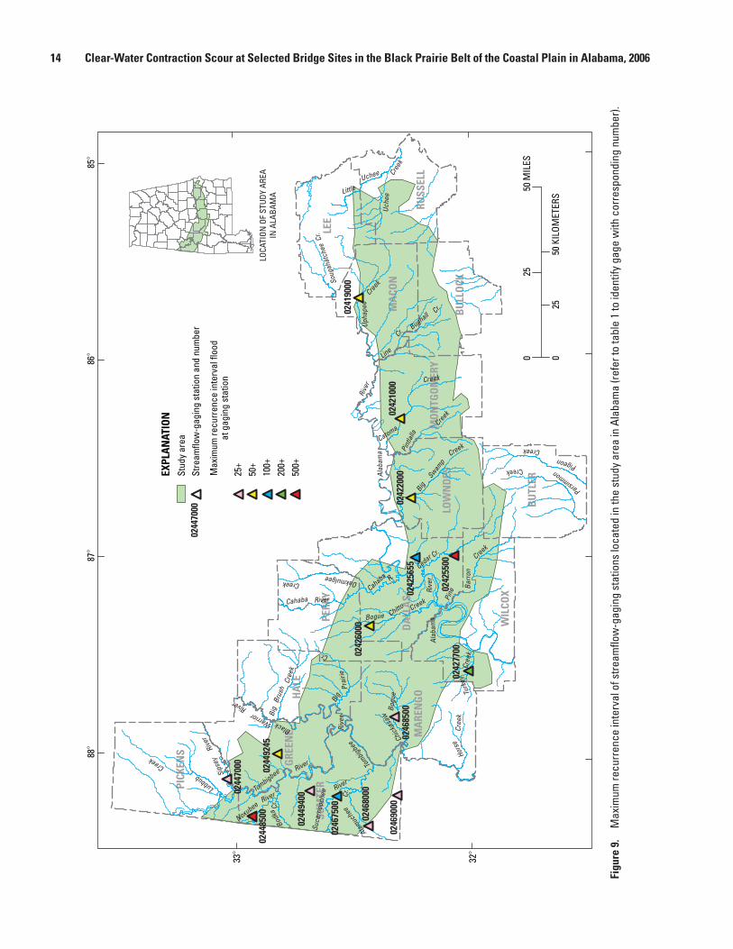
The significant floods in the study area were researched using gage data and flood reports to determine the magnitude and the affected areas. The oldest bridge in the database was constructed during 1925. This date was the starting point for flood research. A primary source of information is the USGS streamgaging network. Current and past streamgages, located in the study area, were inspected for significant events. A log-Pearson Type III frequency analysis was performed for each gage located in the study area and was used with regional regression equations to determine the best weighted estimates of peak flow. This analysis was the basis used for determining the recurrence interval of the most significant peaks of record. Dates of known flooding events also were inspected for each gage. Fifteen gages were selected to represent the flooding history of the study area. These gages recorded a total of 52 peaks that represent flooding ranging from about the 10-year flood to greater than a 500-year flood (table 1). The 52 peaks were specific to 16 different years. Most of the gages showed flooding during 1961, 1979, and 1990. Ten of the gages in the study area have peaks greater than the 50-year recurrence interval flood (fig. 9). The year and geographic location of the floods were compared to the construction dates of the bridges in the database. Correlations were made to determine if the bridges in the database were affected by a significant flood. The probable floods of impact were determined for each scour site and are listed in Appendix 1. The more noteworthy floods (1929, 1951, 1955, 1961, 1964, 1979, and 1990) are presented in more detail later in this report.
There are two types of storms associated with floods in Alabama: frontal systems and tropical storms. The effects of intense precipitation and storm surge of coastal waters associated with tropical storms and hurricanes, thunderstorms, and slow-moving frontal systems usually result in flooding. The flooding potential is increased when rivers and creeks are already swollen with spring runoff. The average annual precipitation varies seasonally and geographically. The statewide average rainfall is about 55 inches and varies from about 50 inches in central and west-central Alabama to about 65 inches near the Gulf of Mexico (Paulson and others, 1991).
Data Assumptions 13
Tabl
e 1.
Ap
prox
imat
e re
curr
ence
inte
rval
for s
elec
ted
flood
yea
rs a
t sel
ecte
d st
ream
flow
-gag
ing
stat
ions
in th
e st
udy
area
in A
laba
ma.
[mi2 ,
squa
re m
ile; A
L, A
laba
ma;
+, p
lus;
—, n
ot a
vaila
ble]
Gag
ing
st
atio
nnu
mbe
rG
agin
g st
atio
n na
me
and
loca
tion
Coun
ty
Dra
in-
age
area
(m
i2 )
Peri
od
ofre
cord
(yea
rs)
1929
1943
1944
1945
1949
1951
1955
1961
1962
1964
1975
1979
1990
1994
1998
2001
0241
9000
Uph
apee
Cre
ek n
ear
Tus
kege
e, A
LM
acon
333
6550
+25
+25
—
25+
—
—
10+
—
50—
—
2
5+10
+10
—
0242
1000
Cat
oma
Cre
ek n
ear
Mon
tgom
ery,
AL
Mon
tgom
ery
290
52—
—
—
—
25
+—
—
5
0+—
—
2
5+—
5
0+—
—
10
+
0242
2000
Big
Sw
amp
Cre
ek n
ear
Low
ndes
boro
, AL
Low
ndes
244
35—
10
+—
—
50
+—
—
25
—
—
—
—
10—
—
—
0242
5500
Ced
ar C
reek
at M
inte
r, A
LD
alla
s21
130
—
—
—
—
—
—
—
100
—
— 5
00+
—
—
—
—
—
0242
5655
Mus
h C
reek
nea
r Se
lma,
AL
Dal
las
44.4
22—
—
—
—
—
—
100
+25
100
25—
—
2
5+—
—
—
0242
6000
Bog
ue C
hitto
Cre
ek n
ear
Bro
wns
, AL
Dal
las
95.4
31—
50
—
—
—
10+
—
—
—
10—
10
—
—
—
—
0242
7700
Tur
key
Cre
ek a
t Kim
brou
gh, A
LW
ilcox
97.5
39—
—
—
—
—
—
—
200
+—
—
—
2
5+ 1
0+—
—
—
0244
7000
Sips
ey R
iver
nea
r Pl
easa
nt R
idge
, AL
Gre
ene
769
22—
—
—
—
—
—
—
25
+—
—
—
—
—
—
—
—
0244
8500
Nox
ubee
Riv
er n
ear
Gei
ger,
AL
Sum
ter
1,09
759
—
—
—
—
10+
—
—
10+
—
—
—
500+
—
—
—
—
0244
9245
Bru
sh C
reek
nea
r E
utaw
, AL
Gre
ene
43.2
26—
—
—
—
—
—
—
—
—
—
—
2
5+ 5
0+—
—
—
0244
9400
Jone
s C
reek
nea
r E
pes,
AL
Sum
ter
11.8
16—
—
—
—
—
—
—
25
+—
—
—
—
—
—
—
—
0246
7500
Suca
rnoo
chee
Riv
er a
t Liv
ings
ton,
AL
Sum
ter
607
64—
—
—
—
—
10
—
10+
—
—
—
100
10+
—
—
—
0246
8000
Ala
muc
hee
Cre
ek n
ear
Cub
a, A
LSu
mte
r62
.317
—
—
—
—
—
—
—
10+
—
25—
2
5+—
—
—
—
0246
8500
Chi
ckas
aw B
ogue
nea
r L
inde
n, A
LM
aren
go25
729
—
—
25+
25+
—
—
—
—
—
—
—
25+
10+
—
—
—
0246
9000
Kin
terb
ish
Cre
ek n
ear
Yor
k, A
LSu
mte
r90
.916
—
—
—
—
—
—
—
10+
—
25+
—
—
—
—
—
—
14 Clear-Water Contraction Scour at Selected Bridge Sites in the Black Prairie Belt of the Coastal Plain in Alabama, 2006
Figu
re 9
. M
axim
um re
curr
ence
inte
rval
of s
tream
flow
-gag
ing
stat
ions
loca
ted
in th
e st
udy
area
in A
laba
ma
(refe
r to
tabl
e 1
to id
entif
y ga
ge w
ith c
orre
spon
ding
num
ber).
HA
LE
PERR
Y
DA
LLA
S
LOW
ND
ESM
ON
TGO
MER
Y
BU
TLER
LEE
RUSS
ELL
WIL
COX
MA
CON
BU
LLO
CK
MA
REN
GO
GRE
ENE
PICK
ENS
SUM
TER
EXPL
AN
ATIO
N
Max
imum
recu
rren
ce in
terv
al fl
ood
at g
agin
g st
atio
n
Stud
y ar
eaSt
ream
flow
-gag
ing
stat
ion
and
num
ber
25+
50+
100+
200+
500+
LOCA
TION
OF
STUD
Y AR
EAIN
ALA
BAM
A
Soug
ahat
chee
Cr.
Uche
e
Uchee
Little
Cree
k
Upha
pee
Cr.
Creek
Line
Bughall Cr.
Creek
Catoma
Pint
lalla
BigSwam
p
Alab
ama
Rive
r
CreekCreek
Alab
ama
Rive
r
Cedar Cr.
Cahaba
Bogue Chitto Creek
R.
Cahaba River Pine
Barr
on
Creek
Turk
eyCr
eek
Hors
eChick
asaw
Cr.
Cree
k
Bogu
e
Big
Big
Brus
h Prai
rie
Tombig
bee
Alamuc
hee
Rive
rCr
.
Suca
rnoo
chee
River
River
Bodk
a
Lubbub
Noxubee
Tombigbee
Cr.River
Creek
Sips
eyBlackWarrio
r
Rive
r
River
Cree
k
OakmulgeeCreek
PersimmonPigeon
Creek
Creek
025
50 K
ILOM
ETER
S
025
50 M
ILES
88
87
86
85
33
32
0244
7000
0244
8500
0244
9245
0244
9400
0246
7500
0246
8000
0246
9000
0246
8500
0242
6000
0242
7700
0242
5655
0242
5500
0242
2000
0242
1000
0241
9000
0244
7000
Data Assumptions 15
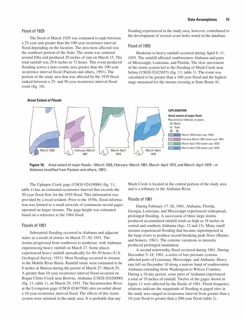
Flood of 1929The flood of March 1929 was estimated to rank between
a 25-year and greater than the 100-year recurrence interval flood depending on the location. The area most affected was the southeast portion of the State. The storm was centered around Elba and produced 20 inches of rain on March 15. The total rainfall was 29.6 inches in 72 hours. This event produced flooding across a nine-county area greater than the 100-year recurrence interval flood (Paulson and others, 1991). The portion of the study area that was affected by the 1929 flood ranked between a 25- and 50-year recurrence interval flood event (fig. 10).
flooding experienced in the study area, however, contributed to the development of several scour holes noted in the database.
Flood of 1955Moderate to heavy rainfall occurred during April 8–11,
1955. The rainfall affected southwestern Alabama and parts of Mississippi, Louisiana, and Florida. The slow movement of the storm system led to the flooding of Mush Creek near Selma (USGS 02425655) (fig. 11; table 1). The event was calculated to be greater than a 100-year flood and the highest stage measured for the stream crossing at State Route 41.
Figure 10. Areal extent of major floods—March 1929, February–March 1961, March–April 1973, and March–April 1979—in Alabama (modified from Paulson and others, 1991).
Mush Creek is located in the central portion of the study area and is a tributary to the Alabama River.
Floods of 1961
During February 17–26, 1961, Alabama, Florida, Georgia, Louisiana, and Mississippi experienced widespread, prolonged flooding. A succession of three large storms produced accumulated rainfall totals as high as 18 inches in central and southern Alabama (figs. 12 and 13). Many small streams experienced flooding that became superimposed in the large rivers to produce record-breaking peak flows (Barnes and Somers, 1961). The extreme variations in intensity produced prolonged inundation.
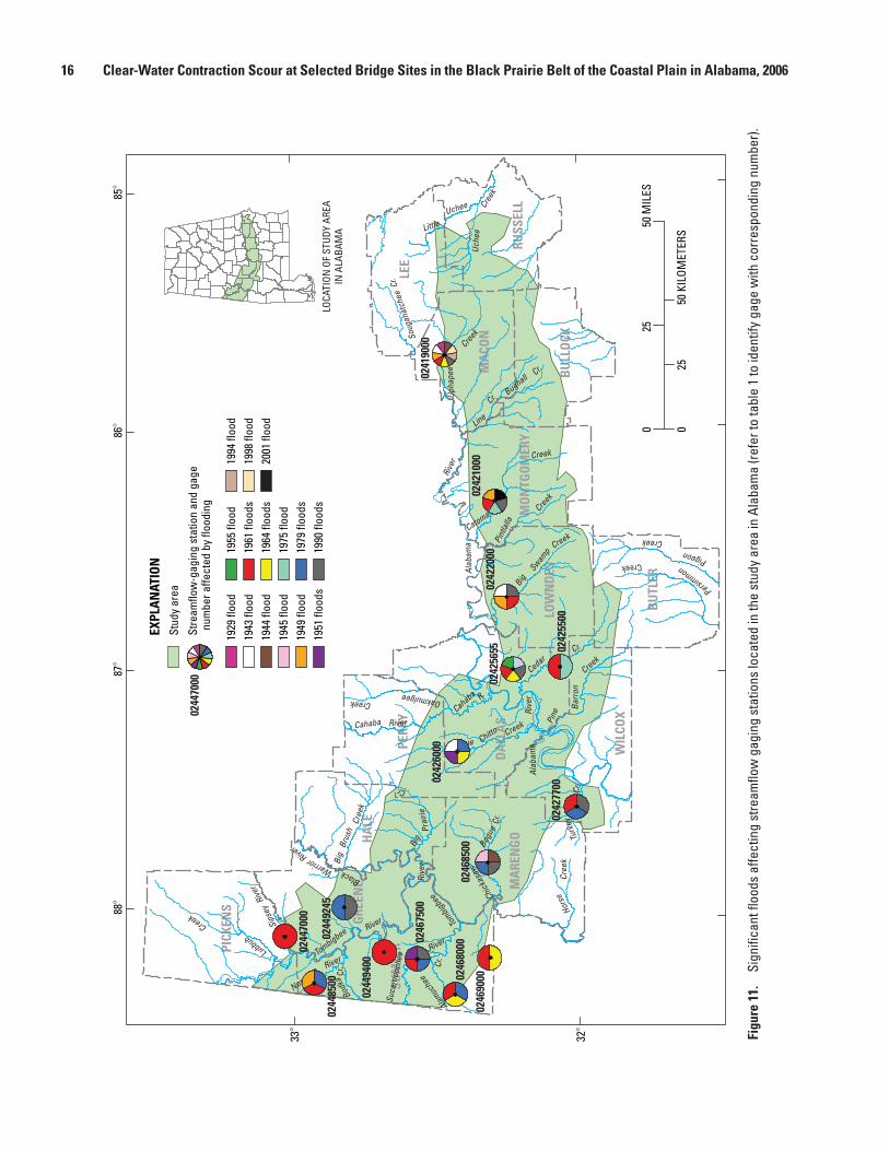
A second noteworthy flood occurred during 1961. During December 5–18, 1961, a series of low-pressure systems affected parts of Louisiana, Mississippi, and Alabama. Heavy rain fell on December 10 along a narrow band of southwestern Alabama extending from Washington to Wilcox Counties. During a 10-day period, some parts of Alabama experienced a total of 19 inches of rainfall. Twelve of the gages shown in figure 11 were affected by the floods of 1961. Flood-frequency relations indicate the magnitude of flooding at gaged sites in the study area ranged in recurrence interval from greater than a 10-year flood to greater than a 200-year flood (table 2).
Areal extent of major flood
EXPLANATION
Areal Extent of Floods
Recurrence interval, in years25to50
Morethan
50March 1929 (water year 1929)
February-March 1961 (water year 1961)
March-April 1973 (water year 1973)
March-April 1979 (water year 1979)March 1929 February-March
1961March-April
1973March-April
1979
The Uphapee Creek gage (USGS 02419000) (fig. 11; table 1) has an estimated recurrence interval that exceeds the 50-year flood flow for the 1929 flood. This information was provided by a local resident. Prior to the 1930s, flood informa-tion was limited to a small network of continuous record gages operated on larger streams. The gage height was estimated based on a reference to the 1964 flood.
Floods of 1951
Substantial flooding occurred in Alabama and adjacent states as a result of storms on March 27–30, 1951. The storms progressed from southwest to northeast, with Alabama experiencing heavy rainfall on March 27. Some places experienced heavy rainfall sporadically for 40–50 hours (U.S. Geological Survey, 1953). Most flooding occurred in streams in the Mobile River Basin. Rainfall totals were estimated to be 8 inches at Marion during the period of March 27–March 29. A greater than 10-year recurrence interval flood occurred on Bogue Chitto Creek near Browns, Alabama (USGS 02426000) (fig. 11; table 1), on March 29, 1951. The Sucarnoochee River at the Livingston gage (USGS 02467500) also recorded about a 10-year recurrence interval flood. The effects of this storm system were minimal in the study area. It is probable that any
16 Clear-Water Contraction Scour at Selected Bridge Sites in the Black Prairie Belt of the Coastal Plain in Alabama, 2006
Figu
re 1
1.
Sign
ifica
nt fl
oods
affe
ctin
g st
ream
flow
gag
ing
stat
ions
loca
ted
in th
e st
udy
area
in A
laba
ma
(refe
r to
tabl
e 1
to id
entif
y ga
ge w
ith c
orre
spon
ding
num
ber).
HA
LE
PERR
Y
DA
LLA
S
LOW
ND
ES
MO
NTG
OM
ERY
BU
TLER
LEE
RUSS
ELL
WIL
COX
MA
CON
BU
LLO
CK
MA
REN
GO
GRE
ENE
PICK
ENS
SUM
TER
LOCA
TION
OF
STUD
Y AR
EAIN
ALA
BAM
A
Soug
ahat
chee
Cr.
Uche
e
Uchee
Little
Cree
k
Upha
pee
Cr.
Creek
Line
Bughall Cr.
Creek
Catoma
Pint
lalla
BigSwam
p
Alab
ama
Rive
r
CreekCreek
Alab
ama
Rive
r
CedarCr.
Cahaba
Bogue Chitto Creek
R.
Cahaba River Pine
Barr
on
Creek
Turk
eyCr
.Ho
rseCh
ickas
aw
Cr.
Cree
k
Bogu
e
Big
Big
Brus
h Prai
rie
Tombig
bee
Alamuc
hee
Rive
r
Cr.
Suca
rnoo
chee
RiverRiver
Bodk
a
Lubbub
Noxubee
Tombigbee
Cr.River
Creek
Sips
eyBlackWarrio
r
Rive
r
River
Cree
k
OakmulgeeCreek
PersimmonPigeon
Creek
Creek
Cr.
025
50 K
ILOM
ETER
S
025
50 M
ILES
88
87
86
85
33
32
0244
7000
0244
8500
0244
9245
0244
9400
0246
7500
0246
8000
0246
9000
0246
8500
0242
6000
0242
7700
0242
5655 02
4255
00
0242
2000
0242
1000
0241
9000
0244
7000
EXPL
AN
ATIO
NSt
udy
area
Stre
amflo
w-g
agin
g st
atio
n an
d ga
ge n
umbe
r affe
cted
by
flood
ing
1929
floo
d19
43 fl
ood
1944
floo
d19
45 fl
ood
1949
floo
d19
51 fl
oods
1955
floo
d19
61 fl
oods
1964
floo
ds19
75 fl
ood
1979
floo
ds19
90 fl
oods
1994
floo
d19
98 fl
ood
2001
floo
d
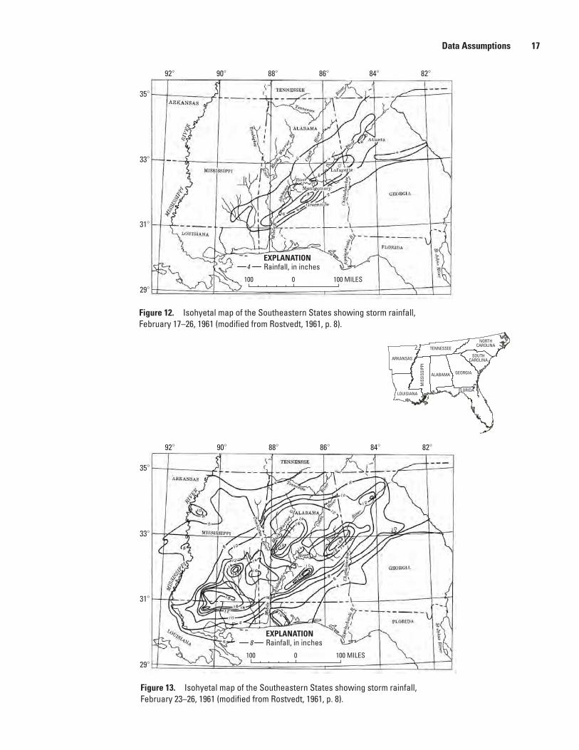
Data Assumptions 17
Figure 12. Isohyetal map of the Southeastern States showing storm rainfall, February 17–26, 1961 (modified from Rostvedt, 1961, p. 8).
Figure 13. Isohyetal map of the Southeastern States showing storm rainfall, February 23–26, 1961 (modified from Rostvedt, 1961, p. 8).
100 0 100 MILES
EXPLANATIONRainfall, in inches4
92 90 88 86 84 82
35
33
31
29
100 0 100 MILES
EXPLANATIONRainfall, in inches8
92 90 88 86 84 82
35
33
31
29
NORTHCAROLINA
SOUTHCAROLINA
GEORGIAALABAMA
LOUISIANA
ARKANSAS
TENNESSEE
MIS
SISS
IPPI
FLORIDA
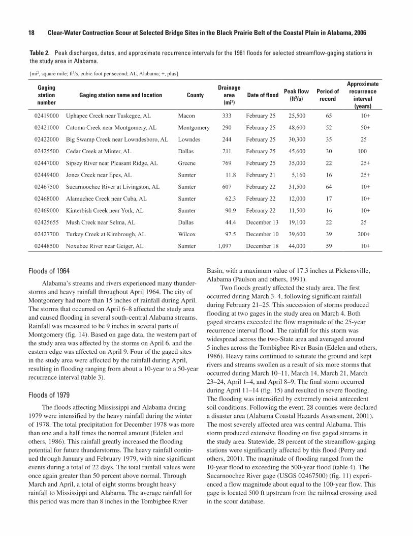
18 Clear-Water Contraction Scour at Selected Bridge Sites in the Black Prairie Belt of the Coastal Plain in Alabama, 2006
Floods of 1964
Alabama’s streams and rivers experienced many thunder-storms and heavy rainfall throughout April 1964. The city of Montgomery had more than 15 inches of rainfall during April. The storms that occurred on April 6–8 affected the study area and caused flooding in several south-central Alabama streams. Rainfall was measured to be 9 inches in several parts of Montgomery (fig. 14). Based on gage data, the western part of the study area was affected by the storms on April 6, and the eastern edge was affected on April 9. Four of the gaged sites in the study area were affected by the rainfall during April, resulting in flooding ranging from about a 10-year to a 50-year recurrence interval (table 3).
Floods of 1979
The floods affecting Mississippi and Alabama during 1979 were intensified by the heavy rainfall during the winter of 1978. The total precipitation for December 1978 was more than one and a half times the normal amount (Edelen and others, 1986). This rainfall greatly increased the flooding potential for future thunderstorms. The heavy rainfall contin-ued through January and February 1979, with nine significant events during a total of 22 days. The total rainfall values were once again greater than 50 percent above normal. Through March and April, a total of eight storms brought heavy rainfall to Mississippi and Alabama. The average rainfall for this period was more than 8 inches in the Tombigbee River
Basin, with a maximum value of 17.3 inches at Pickensville, Alabama (Paulson and others, 1991).
Two floods greatly affected the study area. The first occurred during March 3–4, following significant rainfall during February 21–25. This succession of storms produced flooding at two gages in the study area on March 4. Both gaged streams exceeded the flow magnitude of the 25-year recurrence interval flood. The rainfall for this storm was widespread across the two-State area and averaged around 5 inches across the Tombigbee River Basin (Edelen and others, 1986). Heavy rains continued to saturate the ground and kept rivers and streams swollen as a result of six more storms that occurred during March 10–11, March 14, March 21, March 23–24, April 1–4, and April 8–9. The final storm occurred during April 11–14 (fig. 15) and resulted in severe flooding. The flooding was intensified by extremely moist antecedent soil conditions. Following the event, 28 counties were declared a disaster area (Alabama Coastal Hazards Assessment, 2001). The most severely affected area was central Alabama. This storm produced extensive flooding on five gaged streams in the study area. Statewide, 28 percent of the streamflow-gaging stations were significantly affected by this flood (Perry and others, 2001). The magnitude of flooding ranged from the 10-year flood to exceeding the 500-year flood (table 4). The Sucarnoochee River gage (USGS 02467500) (fig. 11) experi-enced a flow magnitude about equal to the 100-year flow. This gage is located 500 ft upstream from the railroad crossing used in the scour database.
Table 2. Peak discharges, dates, and approximate recurrence intervals for the 1961 floods for selected streamflow-gaging stations in the study area in Alabama.
[mi2, square mile; ft3/s, cubic foot per second; AL, Alabama; +, plus]
Gaging station number
Gaging station name and location CountyDrainage
area(mi2)
Date of floodPeak flow
(ft3/s)Period of
record
Approximate recurrence
interval(years)
02419000 Uphapee Creek near Tuskegee, AL Macon 333 February 25 25,500 65 10+
02421000 Catoma Creek near Montgomery, AL Montgomery 290 February 25 48,600 52 50+
02422000 Big Swamp Creek near Lowndesboro, AL Lowndes 244 February 25 30,300 35 25
02425500 Cedar Creek at Minter, AL Dallas 211 February 25 45,600 30 100
02447000 Sipsey River near Pleasant Ridge, AL Greene 769 February 25 35,000 22 25+
02449400 Jones Creek near Epes, AL Sumter 11.8 February 21 5,160 16 25+
02467500 Sucarnoochee River at Livingston, AL Sumter 607 February 22 31,500 64 10+
02468000 Alamuchee Creek near Cuba, AL Sumter 62.3 February 22 12,000 17 10+
02469000 Kinterbish Creek near York, AL Sumter 90.9 February 22 11,500 16 10+
02425655 Mush Creek near Selma, AL Dallas 44.4 December 13 19,100 22 25
02427700 Turkey Creek at Kimbrough, AL Wilcox 97.5 December 10 39,600 39 200+
02448500 Noxubee River near Geiger, AL Sumter 1,097 December 18 44,000 59 10+
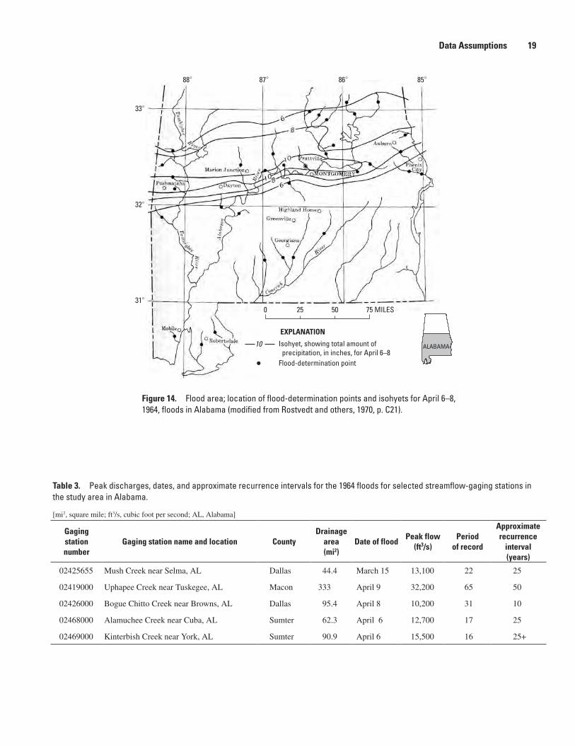
Data Assumptions 19
Figure 14. Flood area; location of flood-determination points and isohyets for April 6–8, 1964, floods in Alabama (modified from Rostvedt and others, 1970, p. C21).
Table 3. Peak discharges, dates, and approximate recurrence intervals for the 1964 floods for selected streamflow-gaging stations in the study area in Alabama.
[mi2, square mile; ft3/s, cubic foot per second; AL, Alabama]
Gaging station number
Gaging station name and location CountyDrainage
area(mi2)
Date of floodPeak flow
(ft3/s)Period
of record
Approximate recurrence
interval(years)
02425655 Mush Creek near Selma, AL Dallas 44.4 March 15 13,100 22 25
02419000 Uphapee Creek near Tuskegee, AL Macon 333 April 9 32,200 65 50
02426000 Bogue Chitto Creek near Browns, AL Dallas 95.4 April 8 10,200 31 10
02468000 Alamuchee Creek near Cuba, AL Sumter 62.3 April 6 12,700 17 25
02469000 Kinterbish Creek near York, AL Sumter 90.9 April 6 15,500 16 25+
0 25 50 75 MILES
EXPLANATION
Isohyet, showing total amount of precipitation, in inches, for April 6–8Flood-determination point
10
33
32
31
88 87 86 85
ALABAMA
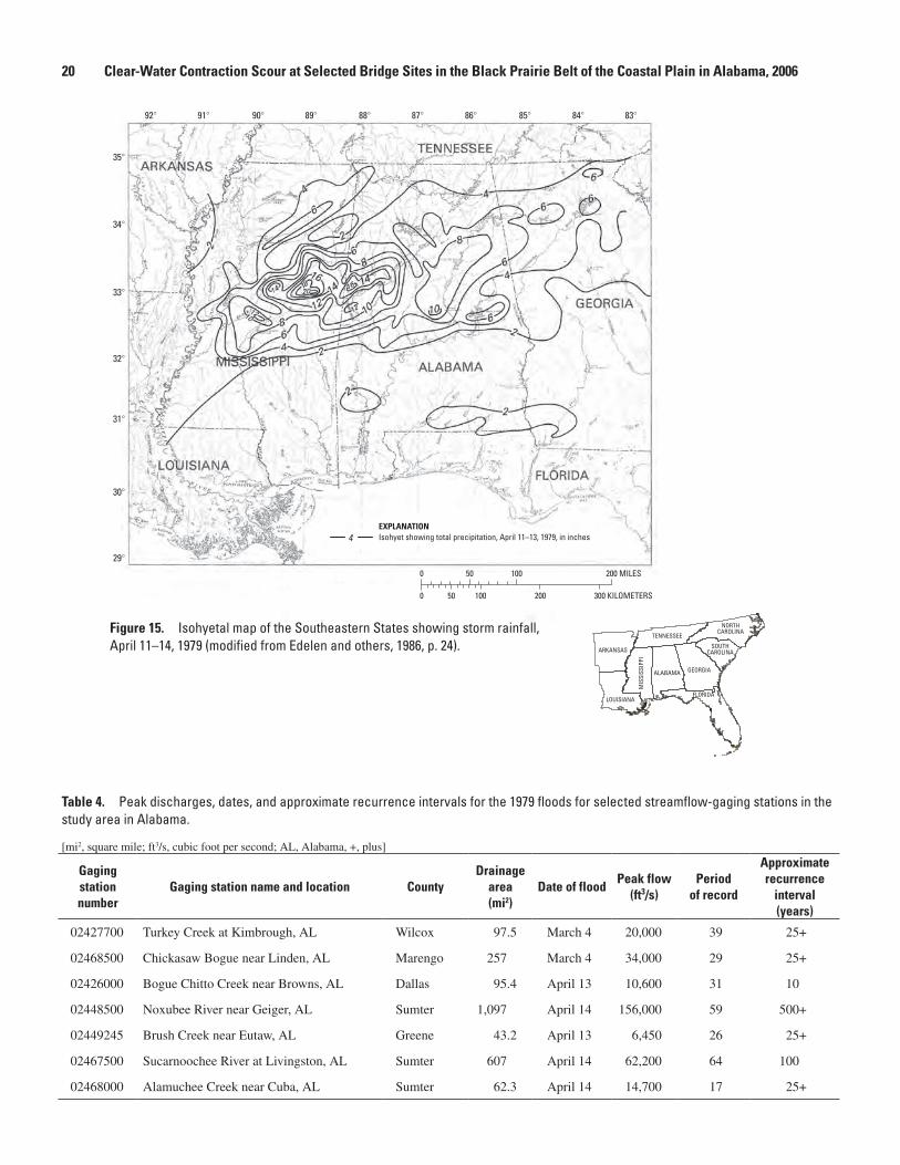
20 Clear-Water Contraction Scour at Selected Bridge Sites in the Black Prairie Belt of the Coastal Plain in Alabama, 2006
Figure 15. Isohyetal map of the Southeastern States showing storm rainfall, April 11–14, 1979 (modified from Edelen and others, 1986, p. 24).
Table 4. Peak discharges, dates, and approximate recurrence intervals for the 1979 floods for selected streamflow-gaging stations in the study area in Alabama.
[mi2, square mile; ft3/s, cubic foot per second; AL, Alabama, +, plus]
Gaging station number
Gaging station name and location CountyDrainage
area(mi2)
Date of floodPeak flow
(ft3/s)Period
of record
Approximate recurrence
interval(years)
02427700 Turkey Creek at Kimbrough, AL Wilcox 97.5 March 4 20,000 39 25+
02468500 Chickasaw Bogue near Linden, AL Marengo 257 March 4 34,000 29 25+
02426000 Bogue Chitto Creek near Browns, AL Dallas 95.4 April 13 10,600 31 10
02448500 Noxubee River near Geiger, AL Sumter 1,097 April 14 156,000 59 500+
02449245 Brush Creek near Eutaw, AL Greene 43.2 April 13 6,450 26 25+
02467500 Sucarnoochee River at Livingston, AL Sumter 607 April 14 62,200 64 100
02468000 Alamuchee Creek near Cuba, AL Sumter 62.3 April 14 14,700 17 25+
0 50 100 200 MILES
0 50 100 200 300 KILOMETERS
EXPLANATIONIsohyet showing total precipitation, April 11–13, 1979, in inches4
35
34
33
32
31
30
29
92 91 90 89 88 87 86 85 84 83
NORTHCAROLINA
SOUTHCAROLINA
GEORGIAALABAMA
LOUISIANA
ARKANSAS
TENNESSEEM
ISSI
SSIP
PI
FLORIDA
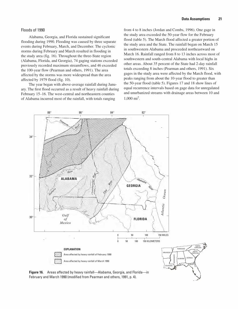
Data Assumptions 21
Floods of 1990
Alabama, Georgia, and Florida sustained significant flooding during 1990. Flooding was caused by three separate events during February, March, and December. The cyclonic storms during February and March resulted in flooding in the study area (fig. 16). Throughout the three-State region (Alabama, Florida, and Georgia), 74 gaging stations exceeded previously recorded maximum streamflows, and 46 exceeded the 100-year flow (Pearman and others, 1991). The area affected by the storms was more widespread than the area affected by 1979 flood (fig. 10).
The year began with above-average rainfall during Janu-ary. The first flood occurred as a result of heavy rainfall during February 15–16. The west-central and northeastern counties of Alabama incurred most of the rainfall, with totals ranging
from 4 to 8 inches (Jordan and Combs, 1996). One gage in the study area exceeded the 50-year flow for the February flood (table 5). The March flood affected a greater portion of the study area and the State. The rainfall began on March 15 in southwestern Alabama and proceeded northeastward on March 16. Rainfall ranged from 8 to 13 inches across most of southwestern and south-central Alabama with local highs in other areas. About 35 percent of the State had 2-day rainfall totals exceeding 8 inches (Pearman and others, 1991). Six gages in the study area were affected by the March flood, with peaks ranging from about the 10-year flood to greater than the 50-year flood (table 5). Figures 17 and 18 show lines of equal recurrence intervals based on gage data for unregulated and unurbanized streams with drainage areas between 10 and
1,000 mi2.
Figure 16. Areas affected by heavy rainfall—Alabama, Georgia, and Florida—in February and March 1990 (modified from Pearman and others, 1991, p. 4).
88 86 84 82
34
32
30
ALABAMA
FLORIDA
GEORGIA
Gulfof
Mexico
Atl
an
tic
Oce
an
0 50 100 150 MILES
0 50 100 150 KILOMETERS
Area affected by heavy rainfall of February 1990
EXPLANATION
Area affected by heavy rainfall of March 1990
NORTHCAROLINA
SOUTHCAROLINA
GEORGIAALABAMA
LOUISIANA
ARKANSAS
TENNESSEE
MIS
SISS
IPPI
FLORIDA
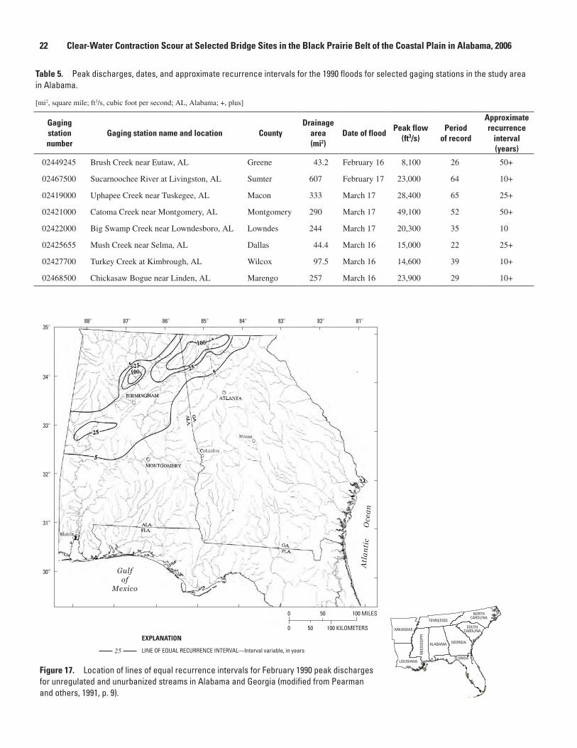
22 Clear-Water Contraction Scour at Selected Bridge Sites in the Black Prairie Belt of the Coastal Plain in Alabama, 2006
Table 5. Peak discharges, dates, and approximate recurrence intervals for the 1990 floods for selected gaging stations in the study area in Alabama.
[mi2, square mile; ft3/s, cubic foot per second; AL, Alabama; +, plus]
Gaging station number
Gaging station name and location CountyDrainage
area(mi2)
Date of floodPeak flow
(ft3/s)Period
of record
Approximate recurrence
interval(years)
02449245 Brush Creek near Eutaw, AL Greene 43.2 February 16 8,100 26 50+
02467500 Sucarnoochee River at Livingston, AL Sumter 607 February 17 23,000 64 10+
02419000 Uphapee Creek near Tuskegee, AL Macon 333 March 17 28,400 65 25+
02421000 Catoma Creek near Montgomery, AL Montgomery 290 March 17 49,100 52 50+
02422000 Big Swamp Creek near Lowndesboro, AL Lowndes 244 March 17 20,300 35 10
02425655 Mush Creek near Selma, AL Dallas 44.4 March 16 15,000 22 25+
02427700 Turkey Creek at Kimbrough, AL Wilcox 97.5 March 16 14,600 39 10+
02468500 Chickasaw Bogue near Linden, AL Marengo 257 March 16 23,900 29 10+
Figure 17. Location of lines of equal recurrence intervals for February 1990 peak discharges for unregulated and unurbanized streams in Alabama and Georgia (modified from Pearman and others, 1991, p. 9).
3588 87 86 85 84 83 82 81
34
33
32
31
30 Gulfof
Mexico
Atl
an
tic
Oce
an
0 50 100 MILES
0 50 100 KILOMETERS
LINE OF EQUAL RECURRENCE INTERVAL—Interval variable, in years
EXPLANATION
25
NORTHCAROLINA
SOUTHCAROLINA
GEORGIAALABAMA
LOUISIANA
ARKANSAS
TENNESSEE
MIS
SISS
IPPI
FLORIDA
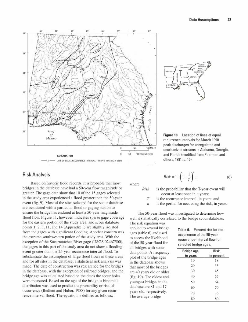
Data Assumptions 23
Risk AnalysisBased on historic flood records, it is probable that most
bridges in the database have had a 50-year flow magnitude or greater. The gage data show that 10 of the 15 gages selected in the study area experienced a flood greater than the 50-year event (fig. 9). Most of the sites selected for the scour database are associated with a particular flood or gaging station to ensure the bridge has endured at least a 50-year magnitude flood flow. Figure 11, however, indicates sparse gage coverage for the eastern portion of the study area, and scour database points 1, 2, 3, 11, and 14 (Appendix 1) are slightly isolated from the gages with significant flooding. Another concern was the extreme southwestern potion of the study area. With the exception of the Sucarnoochee River gage (USGS 02467500), the gages in this part of the study area do not show a flooding event greater than the 25-year recurrence interval flood. To substantiate the assumption of large flood flows in these areas and for all sites in the database, a statistical risk analysis was made. The date of construction was researched for the bridges in the database, with the exception of railroad bridges, and the bridge age was calculated based on the dates the scour holes were measured. Based on the age of the bridge, a binomial distribution was used to predict the probability or risk of occurrence (Bedient and Huber, 1988) for any given recur-rence interval flood. The equation is defined as follows:
where Risk is the probability that the T-year event will
occur at least once in n years; T is the recurrence interval, in years; and n is the period for accessing the risk, in years.
The 50-year flood was investigated to determine how well it statistically correlated to the bridge scour database. The risk equation was applied to several bridge ages (table 6) and used to access the likelihood of the 50-year flood for all bridges with scour data points. A frequency plot of the bridge ages in the database shows that most of the bridges are 40 years old or older (fig. 19). The oldest and youngest bridges in the database are 81 and 17 years old, respectively. The average bridge
Table 6. Percent risk for the occurrence of the 50-year recurrence-interval flow for selected bridge ages.
Bridge age,in years
Risk,in percent
10 18
20 33
30 45
40 55
50 64
60 70
70 76
80 80
(6)
Figure 18. Location of lines of equal recurrence intervals for March 1990 peak discharges for unregulated and unurbanized streams in Alabama, Georgia, and Florida (modified from Pearman and others, 1991, p. 10).
0 50 100 MILES
0 50 100 KILOMETERS
LINE OF EQUAL RECURRENCE INTERVAL—Interval variable, in years
EXPLANATION
5
88 87 86 85 84 83 82 8135
34
33
32
31
30 Gulfof
Mexico
Atl
an
tic
Oce
an
NORTHCAROLINA
SOUTHCAROLINA
GEORGIAALABAMA
LOUISIANA
ARKANSAS
TENNESSEE
MIS
SISS
IPPI
FLORIDA
11 1 ,n
RiskT
= − −
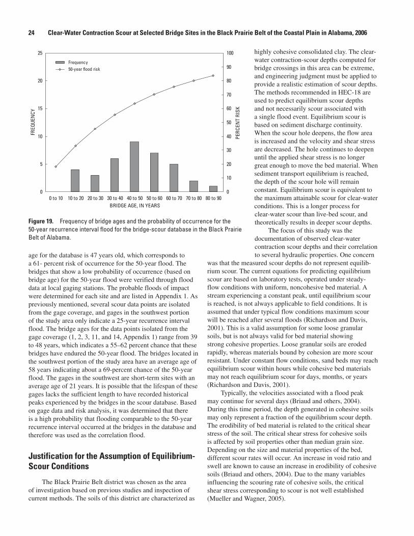
24 Clear-Water Contraction Scour at Selected Bridge Sites in the Black Prairie Belt of the Coastal Plain in Alabama, 2006
age for the database is 47 years old, which corresponds to a 61- percent risk of occurrence for the 50-year flood. The bridges that show a low probability of occurrence (based on bridge age) for the 50-year flood were verified through flood data at local gaging stations. The probable floods of impact were determined for each site and are listed in Appendix 1. As previously mentioned, several scour data points are isolated from the gage coverage, and gages in the southwest portion of the study area only indicate a 25-year recurrence interval flood. The bridge ages for the data points isolated from the gage coverage (1, 2, 3, 11, and 14, Appendix 1) range from 39 to 48 years, which indicates a 55–62 percent chance that these bridges have endured the 50-year flood. The bridges located in the southwest portion of the study area have an average age of 58 years indicating about a 69-percent chance of the 50-year flood. The gages in the southwest are short-term sites with an average age of 21 years. It is possible that the lifespan of these gages lacks the sufficient length to have recorded historical peaks experienced by the bridges in the scour database. Based on gage data and risk analysis, it was determined that there is a high probability that flooding comparable to the 50-year recurrence interval occurred at the bridges in the database and therefore was used as the correlation flood.
Justification for the Assumption of Equilibrium-Scour Conditions
The Black Prairie Belt district was chosen as the area of investigation based on previous studies and inspection of current methods. The soils of this district are characterized as
highly cohesive consolidated clay. The clear-water contraction-scour depths computed for bridge crossings in this area can be extreme, and engineering judgment must be applied to provide a realistic estimation of scour depths. The methods recommended in HEC-18 are used to predict equilibrium scour depths and not necessarily scour associated with a single flood event. Equilibrium scour is based on sediment discharge continuity. When the scour hole deepens, the flow area is increased and the velocity and shear stress are decreased. The hole continues to deepen until the applied shear stress is no longer great enough to move the bed material. When sediment transport equilibrium is reached, the depth of the scour hole will remain constant. Equilibrium scour is equivalent to the maximum attainable scour for clear-water conditions. This is a longer process for clear-water scour than live-bed scour, and theoretically results in deeper scour depths.
The focus of this study was the documentation of observed clear-water contraction scour depths and their correlation to several hydraulic properties. One concern
was that the measured scour depths do not represent equilib-rium scour. The current equations for predicting equilibrium scour are based on laboratory tests, operated under steady-flow conditions with uniform, noncohesive bed material. A stream experiencing a constant peak, until equilibrium scour is reached, is not always applicable to field conditions. It is assumed that under typical flow conditions maximum scour will be reached after several floods (Richardson and Davis, 2001). This is a valid assumption for some loose granular soils, but is not always valid for bed material showing strong cohesive properties. Loose granular soils are eroded rapidly, whereas materials bound by cohesion are more scour resistant. Under constant flow conditions, sand beds may reach equilibrium scour within hours while cohesive bed materials may not reach equilibrium scour for days, months, or years (Richardson and Davis, 2001).
Typically, the velocities associated with a flood peak may continue for several days (Briaud and others, 2004). During this time period, the depth generated in cohesive soils may only represent a fraction of the equilibrium scour depth. The erodibility of bed material is related to the critical shear stress of the soil. The critical shear stress for cohesive soils is affected by soil properties other than median grain size. Depending on the size and material properties of the bed, different scour rates will occur. An increase in void ratio and swell are known to cause an increase in erodibility of cohesive soils (Briaud and others, 2004). Due to the many variables influencing the scouring rate of cohesive soils, the critical shear stress corresponding to scour is not well established (Mueller and Wagner, 2005).
Figure 19. Frequency of bridge ages and the probability of occurrence for the 50-year recurrence interval flood for the bridge-scour database in the Black Prairie Belt of Alabama.
0
5
10
15
20
25
0 to 10 10 to 20 20 to 30 30 to 40 40 to 50 50 to 60 60 to 70 70 to 80 80 to 90BRIDGE AGE, IN YEARS
FREQ
UEN
CY
0
10
20
30
40
50
60
70
80
90
100
PERC
ENT
RISK
Frequency50-year flood risk
Approach 25
Research has been performed to investigate a time-dependent relation between shear stress and erodibility for many cohesive soils. The Erosion Function Apparatus (EFA) has been used to simulate flood velocities ranging from 0 foot per second (ft/s) to 16 ft/s. A curve (erosion function) is developed to describe the relation between the scour rate and shear stress. The critical shear stress also can be determined from the curve. This value indicates the shear stress below which scour will not occur. When the applied shear stress is great enough to exceed the critical shear stress, the bed material begins to scour. This process may have to occur for several floods for equilibrium scour to be attained. Current methods (HEC-18) dictate that the equilibrium scour depth is computed for the 100- and 500-year peak flows. Based on EFA results and the improbability of multiple floods near the 100-year flow occurring, equilibrium scour depths for the 100- and 500-year flows for bridge crossings in Alabama likely will not be attained during the life of the structure.
The Highway Research Center of Auburn University developed erosion functions for selected sites in Alabama using an EFA. An erosion function was developed for the U.S. Highway 84 crossing of Pea River at Elba (Crim and others, 2003). To determine the applicability of equilibrium scour to the cohesive soils in the study area, the erosion functions were used with flood hydrographs to determine the length of time needed for a scour hole to reach equilibrium conditions.
Since the construction of the Pea River Bridge in 1930, the National Weather Service and USGS have operated a streamgaging station at the site. During a period of 77 years (1930–2006), the bridge has experienced four significant floods. The largest recorded flood since the construction of the bridge was the 1990 flood. The estimated peak flow for this event was 58,000 cubic feet per second (ft3/s), which ranks between a 50- and 100-year flood (51,400 ft3/s and 63,500 ft3/s, respectively) (Hedgecock, 2003). Significant flooding also occurred during 1975, 1994, and 1998.
The Pea River Bridge crossing is not located in the study area, but soil samples taken showed similar characteristics to those in the Black Prairie Belt. Three soil samples were collected at different depths from the overbank of the bridge. The measured D
50 values ranged from 0.03 to 0.04 millimeters
(mm), and the soil was about 3 percent clay (Crim and others, 2003). An erosion function was developed for each soil sample by the Highway Research Center. The critical shear stress, critical velocity, and scour rate were determined from the erosion function. The maximum critical shear stress computed for the three samples was 1.5 Newton per square meter
(N/m2). This value corresponds to an approximate critical
velocity of 2.4 ft/s. The HEC-18 methods also were used to compute the
critical velocity for the Pea River Bridge. Based on a particle size of 0.04 mm, the critical velocity was 0.81 ft/s. The
equilibrium scour depth is computed based on bed movement beginning at this velocity. This value is almost three times smaller than the critical velocity computed from the EFA.
The EFA critical velocity value also was used to compute the effective duration of the four floods on Pea River. The effective duration is the time, during the life of the bridge, that the velocity was great enough to move bed material. The one-dimensional flow model, Water-Surface Profile (WSPRO) (Shearman, 1990), was used to estimate the minimum flow that would produce an average velocity greater than the critical velocity. During the life of the bridge, the flow exceeded this value a total of 172 hours. The computed 50-year flood equilibrium scour, based on equations outlined in HEC-18, was 15.3 ft. At the maximum scour rate, from the EFA analysis (3 mm/hour or 0.2362 ft/day), it would take about 1,555 hours to reach equilibrium scour depth. This is under the assumption that the added area from the scour hole would not decrease the velocity and scour rate.
Bridges are designed to withstand scour produced by the 100- and 500-year floods. The largest flooding event occurring during the life of the Pea River Bridge was slightly larger than the 50-year recurrence interval flood. According to EFA data for the Pea River Bridge crossing, the 77-year-old bridge has only experienced 11 percent of the duration needed to produce equilibrium scour for the 50-year flood. This result raises concern of the applicability of laboratory-defined equilibrium scour to cohesive beds. The scour data collected for the database were selected to represent unaltered scour depths located under older bridges having endured a significant flood. The scour depths may not represent HEC-18-defined equi-librium conditions, but provide a good indication of expected scour depths for the typical bridge in the Black Prairie Belt resulting from large floods. The typical bridge would have an expected lifespan of 50 years and would have experienced at least a 50-year recurrence interval flood flow.
Approach
Once the sites were selected for the database and the proper assumptions verified, the necessary field data were collected for the estimation of (1) hypothetical flows, (2) hydraulic data, (3) actual scour depths, and (4) theoretical scour depths. Similar processes are used for hydraulic studies for bridge replacement. To provide consistency, the same techniques were used in the processing and application of the data in this report. The primary difference is that the resulting data were used for the correlation of hydraulic properties to observed scour depths.
26 Clear-Water Contraction Scour at Selected Bridge Sites in the Black Prairie Belt of the Coastal Plain in Alabama, 2006
Estimation of Hydrologic Data
The 50-year recurrence interval flood was determined to be the best-fit hypothetical flood for the scour holes in the database. The 50-year flow was computed for each site unless a larger flood was directly documented for the stream crossing. Each stream crossing and its associated drainage basin were inspected for effects of urbanization. A site visit provided minimal information near the bridge. Aerial photography and land-use data were inspected for urbanization in the entire drainage basin. It was determined that all stream crossings in the database drain areas having little or no urban development. A flood-frequency relation was developed for flood-peak discharges for the 2-, 5-, 10-, 25-, 50-, 100-, 200-, and 500-year recurrence intervals using the procedures described in Magnitude and Frequency of Floods in Alabama, by Atkins, (1996). Flood-peak discharge estimates were computed using the rural regional regression equations for the appropriate hydrologic region. Twenty of the 25 sites are located within flood region 3. The equations for this region produce the highest runoff per square mile in the State. The remaining five sites are located in region 4, just south of the flood region 3 boundary.
Alternative methods were used for computing peak flows for 2 of the 25 sites; USGS streamflow gage data were available at these sites. Flood estimates at gaged sites were determined by weighting the regional and station flood estimates for the specified recurrence interval using the number of years of station record and the accuracy of the regional flood-frequency equations expressed as equivalent years of record (Atkins, 1996).
The Big Swamp Creek gage (USGS 02422000) (fig. 11) was operational for 33 consecutive years and experienced a flood during 1943, 1949, 1961, and 1990. The 1949 flood was slightly larger than the 50-year event. The stream crossing has five structures for the eastbound lanes and five structures for the westbound lanes. All of the structures were examined for the effects of scour. The deepest holes were found under the four relief bridges on the eastbound lanes. These bridges were constructed during 1946 and were affected by the 1948 flood. The 50-year flood was used as the hypothetical flow that contributed to the measured scour. The bridges located on the westbound lanes were constructed during 1982 and did not experience the 1949 flood. These bridges were not included in the database.
The database contains two railroad structures. One of these structures, the Sucarnoochee River bridge, is located 500 ft downstream from a USGS streamflow gage. The Sucarnoochee River gage (UGSG 02467500) has been operational since 1939 and was affected by the 1979 flood. This flood was calculated to be about a 100-year flood event. Based on the 1979 flood, the 100-year flood flow was used as the hypothetical flow for scour correlations. This was the only scour site for which a larger than 50-year recurrence interval flood flow was directly determined.
Estimation of Hydraulic Data
A stage-discharge relation was developed using WSPRO for each site just downstream from the crossing. Water-surface elevations for selected recurrence interval floods were determined using this stage-discharge relation. The same techniques used for bridge replacement studies were used in the construction and execution of the hydraulic models for this study. The models were constructed based on the definition of (1) energy slope, (2) geometry and roughness of floodplain cross sections, and (3) geometry and characteristics of hydraulic structures and associated roadways.
The models were constructed of a series of cross sections (exit, full valley, bridge, and approach) that segment the valley reach into short subreaches (fig. 20). The hydraulic control was identified for each site and the appropriate cross section surveyed, using an electronic total station. In all cases, the normal depth downstream from the crossing was identified as the control. A cross section was defined downstream from the bridge opening to represent the exit section. This cross section represents the section of minimum area and controls the water-surface elevation at the bridge. The starting water-surface elevation was computed at the exit section based on the slope-conveyance method. The geometry was defined at the full valley section, just downstream from the bridge, on natural (prescoured) ground. This section also was used to represent the ground-surface elevations in the bridge opening. This section represents the minimal flow area prior to the effects of scour. The width of the bridge section was determined based on the beginning and ending stations of the bridge and adjusted for the effects of skew. A weir section also was surveyed in the event that the 50-year flood overtopped the roadway.
Many of the sites have relatively uniform reaches without any significant changes in floodplain width. For these sites, the exit section was propagated upstream from the bridge to represent the approach section. Additional cross sections were surveyed for sites that had significant changes in floodplain width.
Eleven of the 25 sites were on U.S. or State routes; for these sites, as-built plans were furnished by ALDOT, which provided prescoured ground elevations near the bridge and showed any modifications to the natural channel route. This information was helpful in determining the authenticity of the scour hole. Recent highway plans included floodplain cross sections that were verified and used in conjunction with the surveyed cross sections.
The assumption was made that each of the bridges in the database has experienced a 50-year flood flow at least once during the life of the structures. This assumption was determined based on the construction date of the bridge and documented floods in the general area. Each site was correlated to a particular flood(s) experienced in the general area (Appendix 1). These flood(s) were considered to be a contributor to the existing scour hole. The conditions reflective of the flooding period were considered in developing the
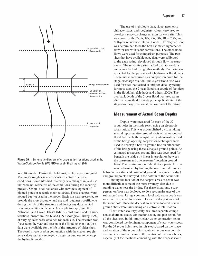
Approach 27
WSPRO model. During the field visit, each site was assigned Manning’s roughness coefficients reflective of current conditions. Some sites had relatively new changes in land use that were not reflective of the conditions during the scouring process. Several sites had areas with new development of planted pines or recently clear-cut areas. These changes were notated but not used in the model. Each site was researched to provide the most accurate land use and roughness coefficients during the life of the structure and during any documented flooding event(s) in the area. Aerial photography and the National Land Cover Dataset (Multi-Resolution Land Charac-teristics Consortium, 2006, and U.S. Geological Survey, 1992) of varying dates were obtained for each site. The research was focused on the year and season of the flooding event(s). Less data were available for the life of the structure of older sites. The results were used in conjunction with the current rough-ness values and any surveyed changes in land use to develop the hydraulic model.
The use of hydrologic data, slope, geometric characteristics, and roughness values were used to develop a stage-discharge relation for each site. This was done for the 2-, 5-, 10-, 25-, 50-, 100-, 200-, and 500-year recurrence interval floods. The 50-year flood was determined to be the best estimated hypothetical flow for use with scour correlations. The other flood flows were used for comparison purposes. The two sites that have available gage data were calibrated to the gage rating, developed through flow measure-ments. The remaining sites lacked calibration data and were checked using other methods. Each site was inspected for the presence of a high-water flood mark. These marks were used as a comparison point for the stage-discharge relation. The 2-year flood also was used for sites that lacked calibration data. Typically for most sites, the 2-year flood is a couple of feet deep in the floodplain (Methods and others, 2003). The overbank depth of the 2-year flood was used as an alternative method for testing the applicability of the stage-discharge relation at the low end of the rating.
Measurement of Actual Scour Depths
Depths were measured for each of the 37 scour holes in the study reach using an electronic total station. This was accomplished by first taking several representative ground shots of the unscoured floodplain on both the upstream and downstream sides of the bridge opening. Regression techniques were used to develop a best-fit ground line on either side of the bridge using these surveyed ground points. An estimated unscoured ground line was developed for beneath the bridge by linear interpolation between the upstream and downstream floodplain ground lines. The maximum scour depth for a particular site was determined by finding the maximum difference
between the estimated unscoured ground line (under bridge) and ground points surveyed in the bottom of the scour hole.
Finding the location of the deepest areas of scour was more difficult at some of the more swampy sites due to standing water near the bridge. For these situations, a two-person jon boat was deployed to do a reconnaissance of the submerged area. Using a common level rod, water depth was measured at several locations to locate the deepest areas of the scour hole. Once the deepest areas were located, several ground shots were taken using an electronic total station.
Clear-water scour typically has three separate compo-nents: abutment scour, contraction scour, and pier scour. For all the sites used in this study, clear-water contraction scour was considered the dominant component of clear-water scour. For the 37 scour holes used in this study, based on the shape and location of the scour holes, abutment scour was consid-ered to be a minimal factor in the creation of the scour holes, especially at the locations coinciding with the deepest scour
Figure 20. Schematic diagram of cross-section locations used in the Water-Surface Profile (WSPRO) model (Shearman, 1990).
Roadway
Approach or start of contraction
Exit or end of expansion
Full valley ordownstream faceof contraction
Bridge or contraction
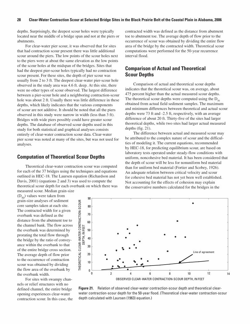
28 Clear-Water Contraction Scour at Selected Bridge Sites in the Black Prairie Belt of the Coastal Plain in Alabama, 2006
depths. Surprisingly, the deepest scour holes were typically located near the middle of a bridge span and not at the piers or abutments.
For clear-water pier scour, it was observed that for sites that had contraction scour present there was little additional scour around the piers. The low points of the scour holes next to the piers were at about the same elevation as the low points of the scour holes at the midspan of the bridges. Sites that had the deepest pier-scour holes typically had no contraction scour present. For these sites, the depth of pier scour was usually from 2 to 3 ft. The deepest clear-water pier-scour hole observed in the study area was 4.6 ft. deep. At this site, there were no other types of scour observed. The largest difference between a pier-scour hole and a neighboring contraction-scour hole was about 2 ft. Usually there was little difference in these depths, which likely indicates that the various components of scour are not additive. It should be noted that all the piers observed in this study were narrow in width (less than 3 ft). Bridges with wide piers possibly could have greater scour depths. The database of observed scour depths used in this study for both statistical and graphical analyses consists entirely of clear-water contraction scour data. Clear-water pier scour was noted at many of the sites, but was not used for analyses.
Computation of Theoretical Scour Depths
Theoretical clear-water contraction scour was computed for each of the 37 bridges using the techniques and equations outlined in HEC-18. The Laursen equation (Richardson and Davis, 2001) (equations 2 and 3) was used to compute the theoretical scour depth for each overbank on which there was measured scour. Median grain-size (D
50) values were taken from
grain-size analyses of sediment core samples taken at each site. The contracted width for a given overbank was defined as the distance from the abutment toe to the channel bank. The flow across the overbank was determined by prorating the total flow through the bridge by the ratio of convey-ance within the overbank to that of the entire bridge cross section. The average depth of flow prior to the occurrence of contraction scour was obtained by dividing the flow area of the overbank by the overbank width.
For sites with swampy chan-nels or relief structures with no defined channel, the entire bridge opening experiences clear-water contraction scour. In this case, the
contracted width was defined as the distance from abutment toe to abutment toe. The average depth of flow prior to the occurrence of scour was obtained by dividing the entire flow area of the bridge by the contracted width. Theoretical scour computations were performed for the 50-year recurrence interval flood.
Comparison of Actual and Theoretical Scour Depths
Comparison of actual and theoretical scour depths indicates that the theoretical scour was, on average, about 475 percent higher than the actual measured scour depths. The theoretical scour depths were computed using the D
50
obtained from actual field sediment samples. The maximum and minimum differences between theoretical and actual scour depths were 73 ft and -2.5 ft, respectively, with an average difference of about 20 ft. Thirty-five of the sites had larger theoretical depths, while two sites had larger actual measured depths (fig. 21).
The difference between actual and measured scour may be attributed to the complex nature of scour and the difficul-ties of modeling it. The current equations, recommended by HEC-18, for predicting equilibrium scour, are based on laboratory tests operated under steady-flow conditions with uniform, noncohesive bed material. It has been considered that the depth of scour will be less for nonuniform bed material than for uniform bed material (Fortier and Scobey, 1926). An adequate relation between critical velocity and scour for cohesive bed material has not yet been well established. Not accounting for the effects of cohesion may explain the conservative numbers calculated for the bridges in the
Figure 21. Relation of observed clear-water contraction-scour depth and theoretical clear-water contraction-scour depth for the 50-year flood. (Theoretical clear-water contraction-scour depth calculated with Laursen (1963) equation.)
0
10
20
30
40
50
60
70
80
90
0 2 4 6 8 10 12 14
OBSERVED CLEAR-WATER CONTRACTION-SCOUR DEPTH, IN FEET
THEO
RETI
CAL
CLEA
R-W
ATER
CON
TRAC
TION
-SCO
UR
DEPT
H, IN
FEE
T
Line of agreement
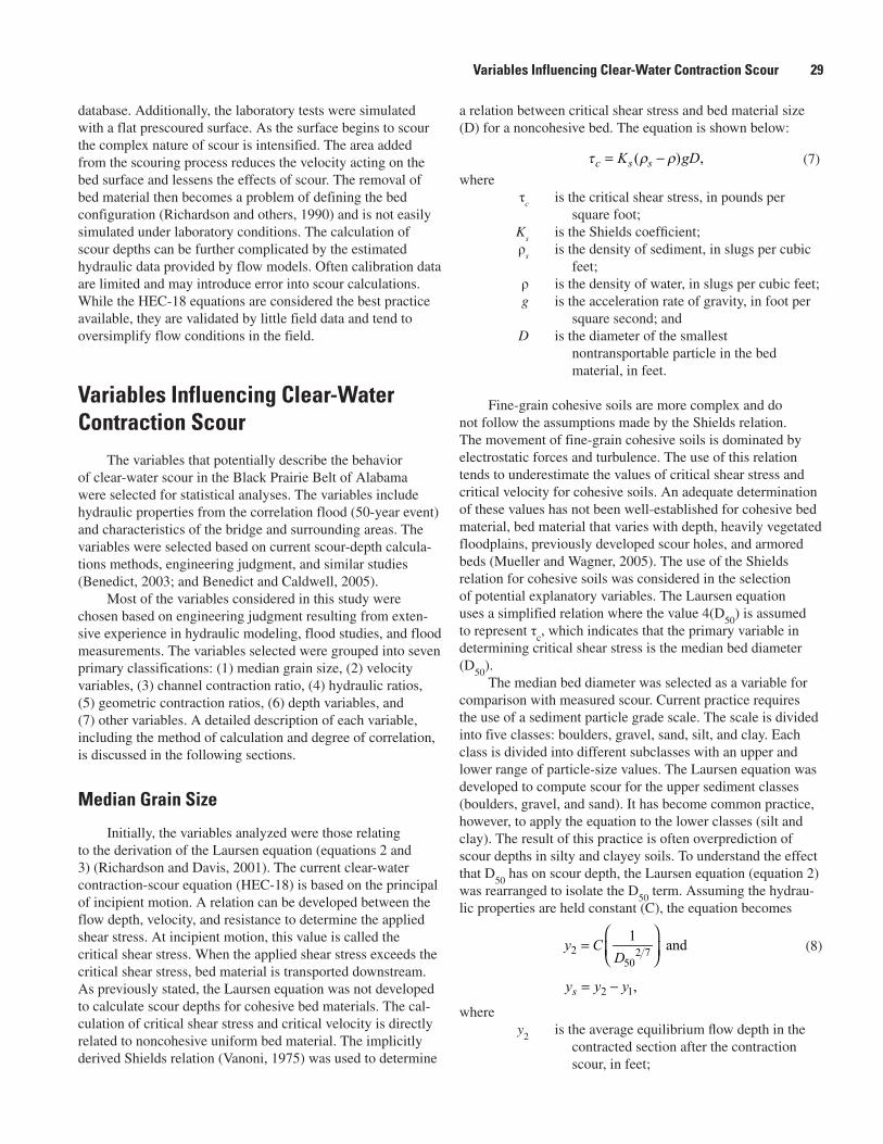
Variables Influencing Clear-Water Contraction Scour 29
database. Additionally, the laboratory tests were simulated with a flat prescoured surface. As the surface begins to scour the complex nature of scour is intensified. The area added from the scouring process reduces the velocity acting on the bed surface and lessens the effects of scour. The removal of bed material then becomes a problem of defining the bed configuration (Richardson and others, 1990) and is not easily simulated under laboratory conditions. The calculation of scour depths can be further complicated by the estimated hydraulic data provided by flow models. Often calibration data are limited and may introduce error into scour calculations. While the HEC-18 equations are considered the best practice available, they are validated by little field data and tend to oversimplify flow conditions in the field.
Variables Influencing Clear-Water Contraction Scour
The variables that potentially describe the behavior of clear-water scour in the Black Prairie Belt of Alabama were selected for statistical analyses. The variables include hydraulic properties from the correlation flood (50-year event) and characteristics of the bridge and surrounding areas. The variables were selected based on current scour-depth calcula-tions methods, engineering judgment, and similar studies (Benedict, 2003; and Benedict and Caldwell, 2005).
Most of the variables considered in this study were chosen based on engineering judgment resulting from exten-sive experience in hydraulic modeling, flood studies, and flood measurements. The variables selected were grouped into seven primary classifications: (1) median grain size, (2) velocity variables, (3) channel contraction ratio, (4) hydraulic ratios, (5) geometric contraction ratios, (6) depth variables, and (7) other variables. A detailed description of each variable, including the method of calculation and degree of correlation, is discussed in the following sections.
Median Grain Size
Initially, the variables analyzed were those relating to the derivation of the Laursen equation (equations 2 and 3) (Richardson and Davis, 2001). The current clear-water contraction-scour equation (HEC-18) is based on the principal of incipient motion. A relation can be developed between the flow depth, velocity, and resistance to determine the applied shear stress. At incipient motion, this value is called the critical shear stress. When the applied shear stress exceeds the critical shear stress, bed material is transported downstream. As previously stated, the Laursen equation was not developed to calculate scour depths for cohesive bed materials. The cal-culation of critical shear stress and critical velocity is directly related to noncohesive uniform bed material. The implicitly derived Shields relation (Vanoni, 1975) was used to determine
a relation between critical shear stress and bed material size (D) for a noncohesive bed. The equation is shown below:
where τ
c is the critical shear stress, in pounds per
square foot; K
s is the Shields coefficient;
ρs is the density of sediment, in slugs per cubic
feet; ρ is the density of water, in slugs per cubic feet; g is the acceleration rate of gravity, in foot per
square second; and D is the diameter of the smallest
nontransportable particle in the bed material, in feet.
Fine-grain cohesive soils are more complex and do not follow the assumptions made by the Shields relation. The movement of fine-grain cohesive soils is dominated by electrostatic forces and turbulence. The use of this relation tends to underestimate the values of critical shear stress and critical velocity for cohesive soils. An adequate determination of these values has not been well-established for cohesive bed material, bed material that varies with depth, heavily vegetated floodplains, previously developed scour holes, and armored beds (Mueller and Wagner, 2005). The use of the Shields relation for cohesive soils was considered in the selection of potential explanatory variables. The Laursen equation uses a simplified relation where the value 4(D
50) is assumed
to represent τc, which indicates that the primary variable in
determining critical shear stress is the median bed diameter (D
50). The median bed diameter was selected as a variable for
comparison with measured scour. Current practice requires the use of a sediment particle grade scale. The scale is divided into five classes: boulders, gravel, sand, silt, and clay. Each class is divided into different subclasses with an upper and lower range of particle-size values. The Laursen equation was developed to compute scour for the upper sediment classes (boulders, gravel, and sand). It has become common practice, however, to apply the equation to the lower classes (silt and clay). The result of this practice is often overprediction of scour depths in silty and clayey soils. To understand the effect that D
50 has on scour depth, the Laursen equation (equation 2)
was rearranged to isolate the D50
term. Assuming the hydrau-lic properties are held constant (C), the equation becomes
where y
2 is the average equilibrium flow depth in the
contracted section after the contraction scour, in feet;
(7)
2 2 750
1 andy CD
=
(8)
2 1,sy y y= −
( ) ,c s sK gD = −
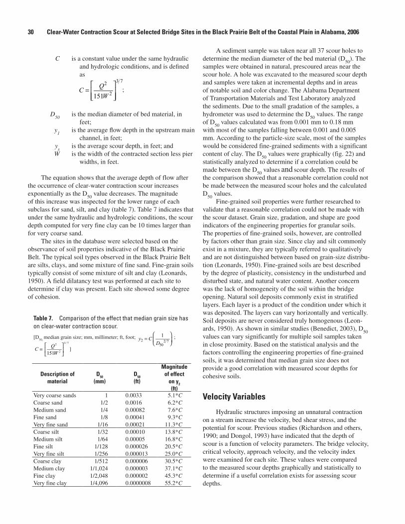
30 Clear-Water Contraction Scour at Selected Bridge Sites in the Black Prairie Belt of the Coastal Plain in Alabama, 2006
C is a constant value under the same hydraulic and hydrologic conditions, and is defined as
D50
is the median diameter of bed material, in feet;
y1
is the average flow depth in the upstream main channel, in feet;
ys is the average scour depth, in feet; and
W is the width of the contracted section less pier widths, in feet.
The equation shows that the average depth of flow after the occurrence of clear-water contraction scour increases exponentially as the D
50 value decreases. The magnitude
of this increase was inspected for the lower range of each subclass for sand, silt, and clay (table 7). Table 7 indicates that under the same hydraulic and hydrologic conditions, the scour depth computed for very fine clay can be 10 times larger than for very coarse sand.
The sites in the database were selected based on the observance of soil properties indicative of the Black Prairie Belt. The typical soil types observed in the Black Prairie Belt are silts, clays, and some mixture of fine sand. Fine-grain soils typically consist of some mixture of silt and clay (Leonards, 1950). A field dilatancy test was performed at each site to determine if clay was present. Each site showed some degree of cohesion.
A sediment sample was taken near all 37 scour holes to determine the median diameter of the bed material (D
50). The
samples were obtained in natural, prescoured areas near the scour hole. A hole was excavated to the measured scour depth and samples were taken at incremental depths and in areas of notable soil and color change. The Alabama Department of Transportation Materials and Test Laboratory analyzed the sediments. Due to the small gradation of the samples, a hydrometer was used to determine the D
50 values. The range
of D50
values calculated was from 0.001 mm to 0.18 mm with most of the samples falling between 0.001 and 0.005 mm. According to the particle-size scale, most of the samples would be considered fine-grained sediments with a significant content of clay. The D
50 values were graphically (fig. 22) and
statistically analyzed to determine if a correlation could be made between the D
50 values
and
scour depth. The results of
the comparison showed that a reasonable correlation could not be made between the measured scour holes and the calculated D
50 values.
Fine-grained soil properties were further researched to validate that a reasonable correlation could not be made with the scour dataset. Grain size, gradation, and shape are good indicators of the engineering properties for granular soils. The properties of fine-grained soils, however, are controlled by factors other than grain size. Since clay and silt commonly exist in a mixture, they are typically referred to qualitatively and are not distinguished between based on grain-size distribu-tion (Leonards, 1950). Fine-grained soils are best described by the degree of plasticity, consistency in the undisturbed and disturbed state, and natural water content. Another concern was the lack of homogeneity of the soil within the bridge opening. Natural soil deposits commonly exist in stratified layers. Each layer is a product of the condition under which it was deposited. The layers can vary horizontally and vertically. Soil deposits are never considered truly homogenous (Leon-ards, 1950). As shown in similar studies (Benedict, 2003), D
50
values can vary significantly for multiple soil samples taken in close proximity. Based on the statistical analysis and the factors controlling the engineering properties of fine-grained soils, it was determined that median grain size does not provide a good correlation with measured scour depths for cohesive soils.
Velocity Variables
Hydraulic structures imposing an unnatural contraction on a stream increase the velocity, bed shear stress, and the potential for scour. Previous studies (Richardson and others, 1990; and Dongol, 1993) have indicated that the depth of scour is a function of velocity parameters. The bridge velocity, critical velocity, approach velocity, and the velocity index were examined for each site. These values were compared to the measured scour depths graphically and statistically to determine if a useful correlation exists for assessing scour depths.
3 72
2151QC
W
=
Table 7. Comparison of the effect that median grain size has on clear-water contraction scour.
[D50,
median grain size; mm, millimeter; ft, foot; ;
C = 7/3
2
2
151
W
Q]
Description of material
D50
(mm)D50
(ft)
Magnitude of effect
on y2
(ft)Very coarse sands 1 0.0033 5.1*CCoarse sand 1/2 0.0016 6.2*CMedium sand 1/4 0.00082 7.6*CFine sand 1/8 0.00041 9.3*CVery fine sand 1/16 0.00021 11.3*CCoarse silt 1/32 0.00010 13.8*CMedium silt 1/64 0.00005 16.8*CFine silt 1/128 0.000026 20.5*CVery fine silt 1/256 0.000013 25.0*CCoarse clay 1/512 0.000006 30.5*CMedium clay 1/1,024 0.000003 37.1*CFine clay 1/2,048 0.000002 45.3*CVery fine clay 1/4,096 0.0000008 55.2*C
;
2 2 750
1 andy CD
=
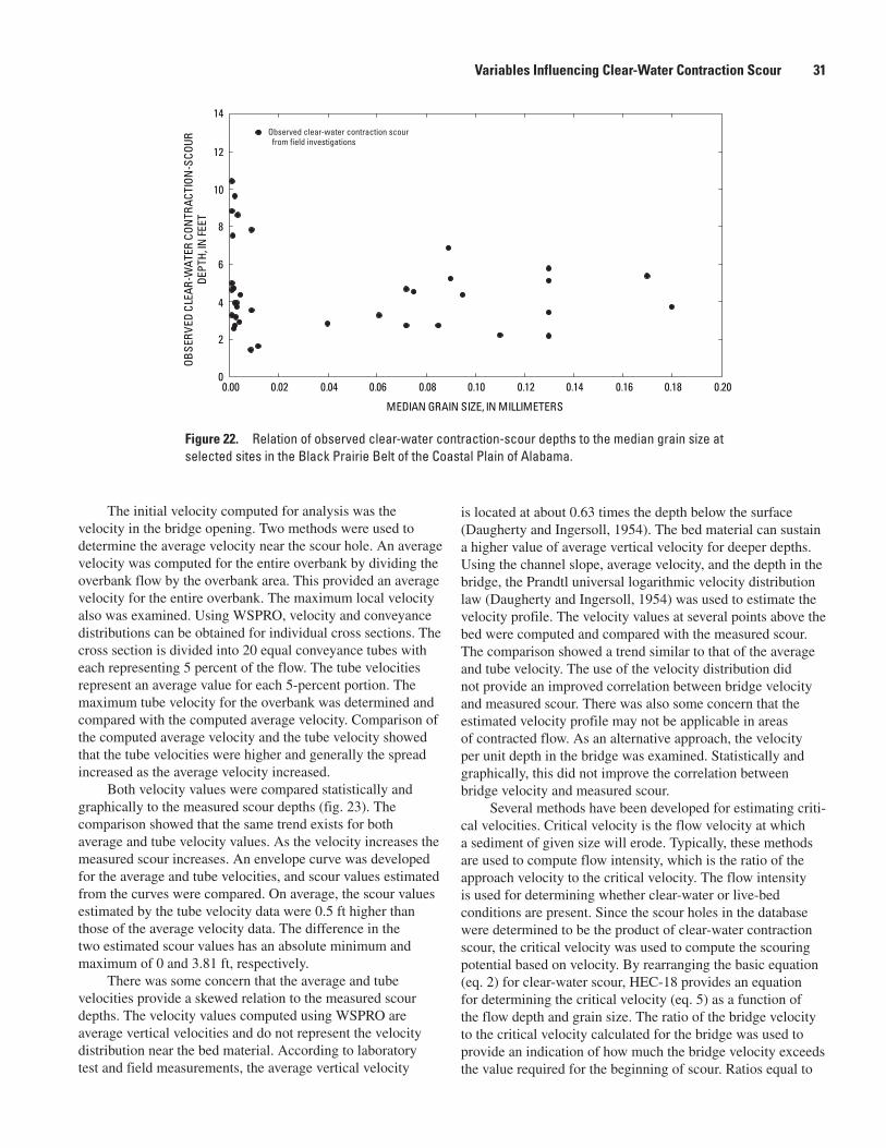
Variables Influencing Clear-Water Contraction Scour 31
The initial velocity computed for analysis was the velocity in the bridge opening. Two methods were used to determine the average velocity near the scour hole. An average velocity was computed for the entire overbank by dividing the overbank flow by the overbank area. This provided an average velocity for the entire overbank. The maximum local velocity also was examined. Using WSPRO, velocity and conveyance distributions can be obtained for individual cross sections. The cross section is divided into 20 equal conveyance tubes with each representing 5 percent of the flow. The tube velocities represent an average value for each 5-percent portion. The maximum tube velocity for the overbank was determined and compared with the computed average velocity. Comparison of the computed average velocity and the tube velocity showed that the tube velocities were higher and generally the spread increased as the average velocity increased.
Both velocity values were compared statistically and graphically to the measured scour depths (fig. 23). The comparison showed that the same trend exists for both average and tube velocity values. As the velocity increases the measured scour increases. An envelope curve was developed for the average and tube velocities, and scour values estimated from the curves were compared. On average, the scour values estimated by the tube velocity data were 0.5 ft higher than those of the average velocity data. The difference in the two estimated scour values has an absolute minimum and maximum of 0 and 3.81 ft, respectively.
There was some concern that the average and tube velocities provide a skewed relation to the measured scour depths. The velocity values computed using WSPRO are average vertical velocities and do not represent the velocity distribution near the bed material. According to laboratory test and field measurements, the average vertical velocity
is located at about 0.63 times the depth below the surface (Daugherty and Ingersoll, 1954). The bed material can sustain a higher value of average vertical velocity for deeper depths. Using the channel slope, average velocity, and the depth in the bridge, the Prandtl universal logarithmic velocity distribution law (Daugherty and Ingersoll, 1954) was used to estimate the velocity profile. The velocity values at several points above the bed were computed and compared with the measured scour. The comparison showed a trend similar to that of the average and tube velocity. The use of the velocity distribution did not provide an improved correlation between bridge velocity and measured scour. There was also some concern that the estimated velocity profile may not be applicable in areas of contracted flow. As an alternative approach, the velocity per unit depth in the bridge was examined. Statistically and graphically, this did not improve the correlation between bridge velocity and measured scour.
Several methods have been developed for estimating criti-cal velocities. Critical velocity is the flow velocity at which a sediment of given size will erode. Typically, these methods are used to compute flow intensity, which is the ratio of the approach velocity to the critical velocity. The flow intensity is used for determining whether clear-water or live-bed conditions are present. Since the scour holes in the database were determined to be the product of clear-water contraction scour, the critical velocity was used to compute the scouring potential based on velocity. By rearranging the basic equation (eq. 2) for clear-water scour, HEC-18 provides an equation for determining the critical velocity (eq. 5) as a function of the flow depth and grain size. The ratio of the bridge velocity to the critical velocity calculated for the bridge was used to provide an indication of how much the bridge velocity exceeds the value required for the beginning of scour. Ratios equal to
Figure 22. Relation of observed clear-water contraction-scour depths to the median grain size at selected sites in the Black Prairie Belt of the Coastal Plain of Alabama.
0.00 0.02 0.04 0.06 0.08 0.10 0.12 0.14 0.16 0.18 0.20
MEDIAN GRAIN SIZE, IN MILLIMETERS
0
2
4
6
8
10
12
14
OBSE
RVED
CLE
AR-W
ATER
CON
TRAC
TION
-SCO
URDE
PTH,
IN FE
ET
Observed clear-water contraction scour from field investigations
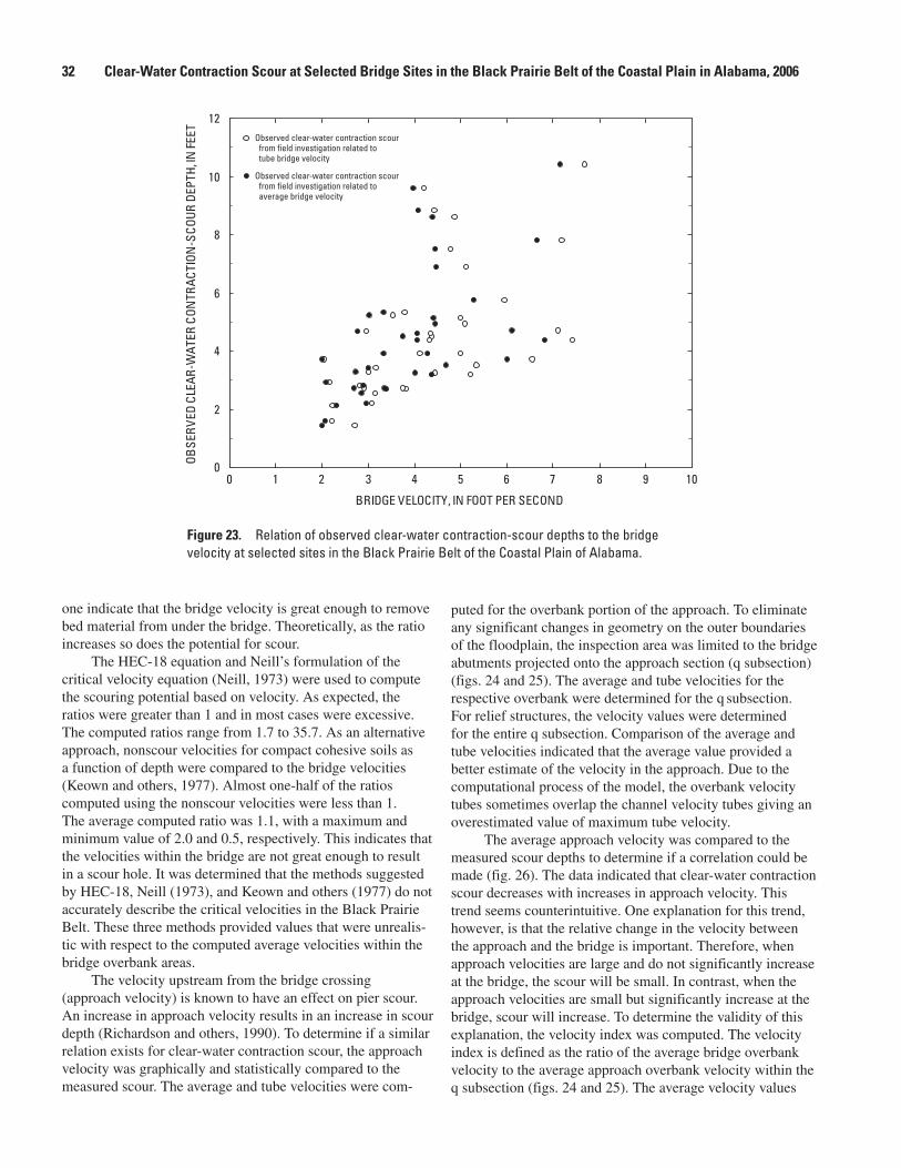
32 Clear-Water Contraction Scour at Selected Bridge Sites in the Black Prairie Belt of the Coastal Plain in Alabama, 2006
one indicate that the bridge velocity is great enough to remove bed material from under the bridge. Theoretically, as the ratio increases so does the potential for scour.
The HEC-18 equation and Neill’s formulation of the critical velocity equation (Neill, 1973) were used to compute the scouring potential based on velocity. As expected, the ratios were greater than 1 and in most cases were excessive. The computed ratios range from 1.7 to 35.7. As an alternative approach, nonscour velocities for compact cohesive soils as a function of depth were compared to the bridge velocities (Keown and others, 1977). Almost one-half of the ratios computed using the nonscour velocities were less than 1. The average computed ratio was 1.1, with a maximum and minimum value of 2.0 and 0.5, respectively. This indicates that the velocities within the bridge are not great enough to result in a scour hole. It was determined that the methods suggested by HEC-18, Neill (1973), and Keown and others (1977) do not accurately describe the critical velocities in the Black Prairie Belt. These three methods provided values that were unrealis-tic with respect to the computed average velocities within the bridge overbank areas.
The velocity upstream from the bridge crossing (approach velocity) is known to have an effect on pier scour. An increase in approach velocity results in an increase in scour depth (Richardson and others, 1990). To determine if a similar relation exists for clear-water contraction scour, the approach velocity was graphically and statistically compared to the measured scour. The average and tube velocities were com-
puted for the overbank portion of the approach. To eliminate any significant changes in geometry on the outer boundaries of the floodplain, the inspection area was limited to the bridge abutments projected onto the approach section (q subsection) (figs. 24 and 25). The average and tube velocities for the respective overbank were determined for the q
subsection.
For relief structures, the velocity values were determined for the entire q subsection. Comparison of the average and tube velocities indicated that the average value provided a better estimate of the velocity in the approach. Due to the computational process of the model, the overbank velocity tubes sometimes overlap the channel velocity tubes giving an overestimated value of maximum tube velocity.
The average approach velocity was compared to the measured scour depths to determine if a correlation could be made (fig. 26). The data indicated that clear-water contraction scour decreases with increases in approach velocity. This trend seems counterintuitive. One explanation for this trend, however, is that the relative change in the velocity between the approach and the bridge is important. Therefore, when approach velocities are large and do not significantly increase at the bridge, the scour will be small. In contrast, when the approach velocities are small but significantly increase at the bridge, scour will increase. To determine the validity of this explanation, the velocity index was computed. The velocity index is defined as the ratio of the average bridge overbank velocity to the average approach overbank velocity within the q subsection (figs. 24 and 25). The average velocity values
Figure 23. Relation of observed clear-water contraction-scour depths to the bridge velocity at selected sites in the Black Prairie Belt of the Coastal Plain of Alabama.
0
2
4
6
8
10
12
0 1 2 3 4 5 6 7 8 9 10
BRIDGE VELOCITY, IN FOOT PER SECOND
OBSE
RVED
CLE
AR-W
ATER
CON
TRAC
TION
-SCO
UR D
EPTH
, IN FE
ET Observed clear-water contraction scour from field investigation related to tube bridge velocity
Observed clear-water contraction scour from field investigation related to average bridge velocity
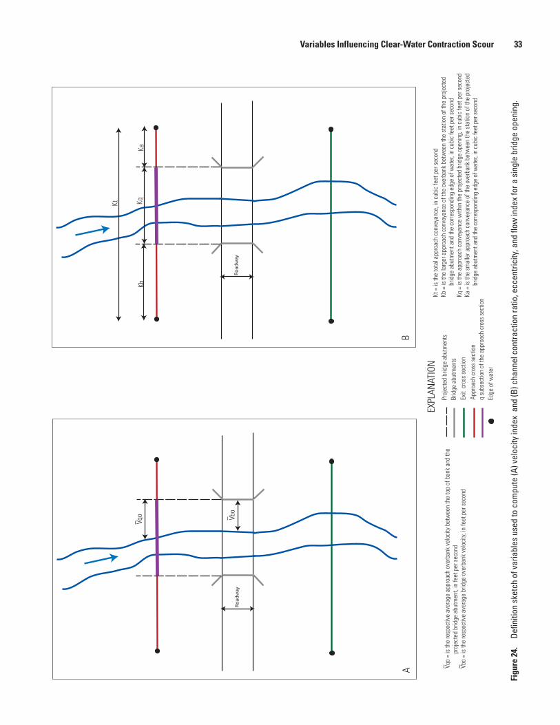
Variables Influencing Clear-Water Contraction Scour 33
Figu
re 2
4.
Defin
ition
ske
tch
of v
aria
bles
use
d to
com
pute
(A) v
eloc
ity in
dex
and
(B) c
hann
el c
ontra
ctio
n ra
tio, e
ccen
trici
ty, a
nd fl
ow in
dex
for a
sin
gle
brid
ge o
peni
ng.
Exit
cro
ss s
ectio
nAp
proa
ch c
ross
sec
tion
Ro
adw
ay
Kt KqKb
Ka
EXPL
ANAT
ION
Proj
ecte
d br
idge
abu
tmen
ts
Edge
of w
ater
Ro
adw
ay
Vqo Vb
o
AB
Brid
ge a
butm
ents
Kt =
is th
e to
tal a
ppro
ach
conv
eyan
ce, i
n cu
bic
feet
per
sec
ond
Kb =
is th
e la
rger
app
roac
h co
nvey
ance
of t
he o
verb
ank
betw
een
the
stat
ion
of th
e pr
ojec
ted
brid
ge a
butm
ent a
nd th
e co
rresp
ondi
ng e
dge
of w
ater
, in
cubi
c fe
et p
er s
econ
dKq
= is
the
appr
oach
con
veya
nce
with
in th
e pr
ojec
ted
brid
ge o
peni
ng, i
n cu
bic
feet
per
sec
ond
Ka =
is th
e sm
alle
r app
roac
h co
nvey
ance
of t
he o
verb
ank
betw
een
the
stat
ion
of th
e pr
ojec
ted
brid
ge a
butm
ent a
nd th
e co
rresp
ondi
ng e
dge
of w
ater
, in
cubi
c fe
et p
er s
econ
d
Vqo
= is
the
resp
ectiv
e av
erag
e ap
proa
ch o
verb
ank
velo
city
bet
wee
n th
e to
p of
ban
k an
d th
e
pro
ject
ed b
ridge
abu
tmen
t, in
feet
per
sec
ond
Vbo
= is
the
resp
ectiv
e av
erag
e br
idge
ove
rban
k ve
loci
ty, i
n fe
et p
er s
econ
d
q
subs
ectio
n of
the
appr
oach
cro
ss s
ectio
n
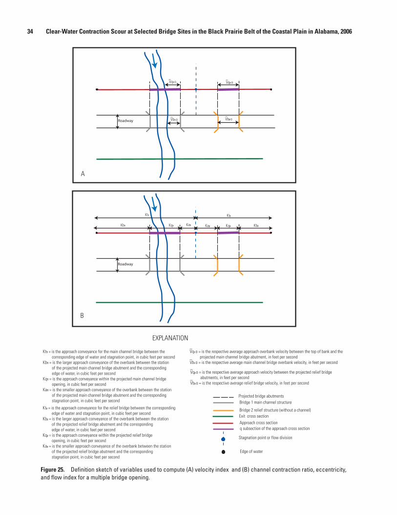
34 Clear-Water Contraction Scour at Selected Bridge Sites in the Black Prairie Belt of the Coastal Plain in Alabama, 2006
Figure 25. Definition sketch of variables used to compute (A) velocity index and (B) channel contraction ratio, eccentricity, and flow index for a multiple bridge opening.
Roadway
Vq1 o
EXPLANATION
Edge of water
Vq2 o
Stagnation point or flow division
Exit cross sectionApproach cross section
Projected bridge abutments
q subsection of the approach cross section
Bridge 1 main channel structure
Roadway
Kt1
Kq1 Ka1 Kq2Ka2 Kb2
Kt2
Kb1
Vb1 o
Bridge 2 relief structure (without a channel)
Vb2 o
Kt1 = is the approach conveyance for the main channel bridge between the corresponding edge of water and stagnation point, in cubic feet per secondKb1 = is the larger approach conveyance of the overbank between the station of the projected main channel bridge abutment and the corresponding edge of water, in cubic feet per secondKq1 = is the approach conveyance within the projected main channel bridge opening, in cubic feet per secondKa1 = is the smaller approach conveyance of the overbank between the station of the projected main channel bridge abutment and the corresponding stagnation point, in cubic feet per second
A
B
Kt2 = is the approach conveyance for the relief bridge between the corresponding edge of water and stagnation point, in cubic feet per secondKb2 = is the larger approach conveyance of the overbank between the station of the projected relief bridge abutment and the corresponding edge of water, in cubic feet per secondKq2 = is the approach conveyance within the projected relief bridge opening, in cubic feet per secondKa2 = is the smaller approach conveyance of the overbank between the station of the projected relief bridge abutment and the corresponding stagnation point, in cubic feet per second
Vq1 o = is the respective average approach overbank velocity between the top of bank and the projected main channel bridge abutment, in feet per secondVb1 o = is the respective average main channel bridge overbank velocity, in feet per second
Vq2 o = is the respective average approach velocity between the projected relief bridge abutments, in feet per secondVb2 o = is the respective average relief bridge velocity, in feet per second
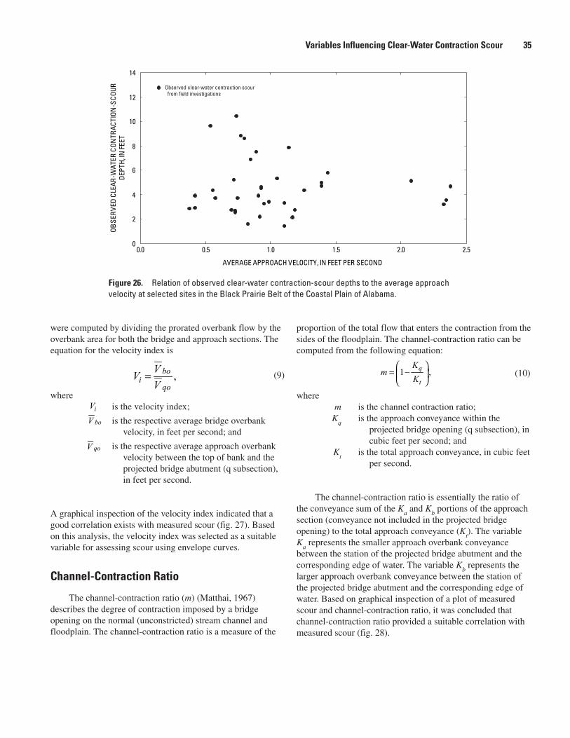
Variables Influencing Clear-Water Contraction Scour 35
were computed by dividing the prorated overbank flow by the overbank area for both the bridge and approach sections. The equation for the velocity index is
where is the velocity index;
is the respective average bridge overbank velocity, in feet per second; and
is the respective average approach overbank velocity between the top of bank and the projected bridge abutment (q subsection), in feet per second.
A graphical inspection of the velocity index indicated that a good correlation exists with measured scour (fig. 27). Based on this analysis, the velocity index was selected as a suitable variable for assessing scour using envelope curves.
Channel-Contraction Ratio
The channel- contraction ratio (m) (Matthai, 1967) describes the degree of contraction imposed by a bridge opening on the normal (unconstricted) stream channel and floodplain. The channel-contraction ratio is a measure of the
proportion of the total flow that enters the contraction from the sides of the floodplain. The channel-contraction ratio can be computed from the following equation:
where m is the channel contraction ratio; K
q is the approach conveyance within the
projected bridge opening (q subsection), in cubic feet per second; and
Kt is the total approach conveyance, in cubic feet
per second.
The channel-contraction ratio is essentially the ratio of the conveyance sum of the K
a and K
b portions of the approach
section (conveyance not included in the projected bridge opening) to the total approach conveyance (K
t). The variable
Ka represents the smaller approach overbank conveyance
between the station of the projected bridge abutment and the corresponding edge of water. The variable K
b represents the
larger approach overbank conveyance between the station of the projected bridge abutment and the corresponding edge of water. Based on graphical inspection of a plot of measured scour and channel-contraction ratio, it was concluded that channel-contraction ratio provided a suitable correlation with measured scour (fig. 28).
Figure 26. Relation of observed clear-water contraction-scour depths to the average approach velocity at selected sites in the Black Prairie Belt of the Coastal Plain of Alabama.
,boi
qo
VVV
=
boV
qoV
iV
(9) 1 ,q
t
Km
K
= −
(10)
0
2
4
6
8
10
12
14
0.0 0.5 1.0 1.5 2.0 2.5
AVERAGE APPROACH VELOCITY, IN FEET PER SECOND
OBSE
RVED
CLE
AR-W
ATER
CON
TRAC
TION
-SCO
URDE
PTH,
IN FE
ET
Observed clear-water contraction scour from field investigations
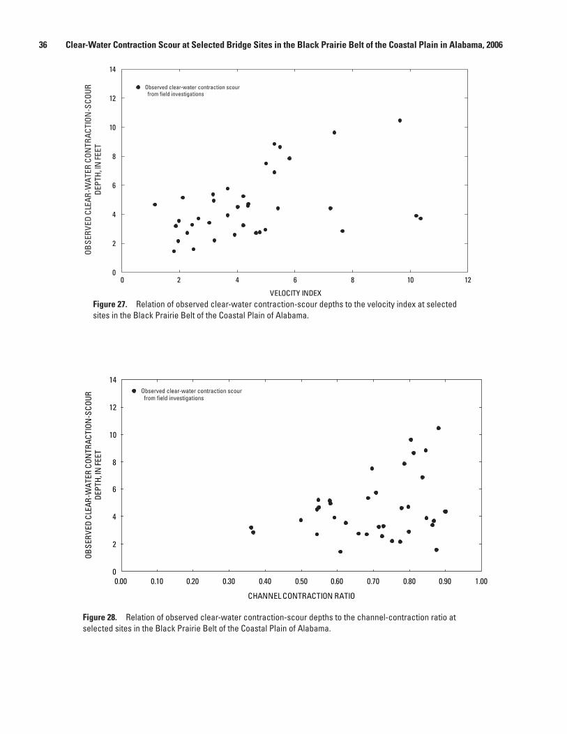
36 Clear-Water Contraction Scour at Selected Bridge Sites in the Black Prairie Belt of the Coastal Plain in Alabama, 2006
Figure 27. Relation of observed clear-water contraction-scour depths to the velocity index at selected sites in the Black Prairie Belt of the Coastal Plain of Alabama.
Figure 28. Relation of observed clear-water contraction-scour depths to the channel-contraction ratio at selected sites in the Black Prairie Belt of the Coastal Plain of Alabama.
OBSE
RVED
CLE
AR-W
ATER
CON
TRAC
TION
-SCO
URDE
PTH,
IN FE
ETObserved clear-water contraction scour from field investigations
0
2
4
6
8
10
12
14
0 2 4 6 8 10 12
VELOCITY INDEX
0
2
4
6
8
10
12
14
0.00 0.10 0.20 0.30 0.40 0.50 0.60 0.70 0.80 0.90 1.00
CHANNEL CONTRACTION RATIO
OBSE
RVED
CLE
AR-W
ATER
CON
TRAC
TION
-SCO
URDE
PTH,
IN FE
ET
Observed clear-water contraction scour from field investigations
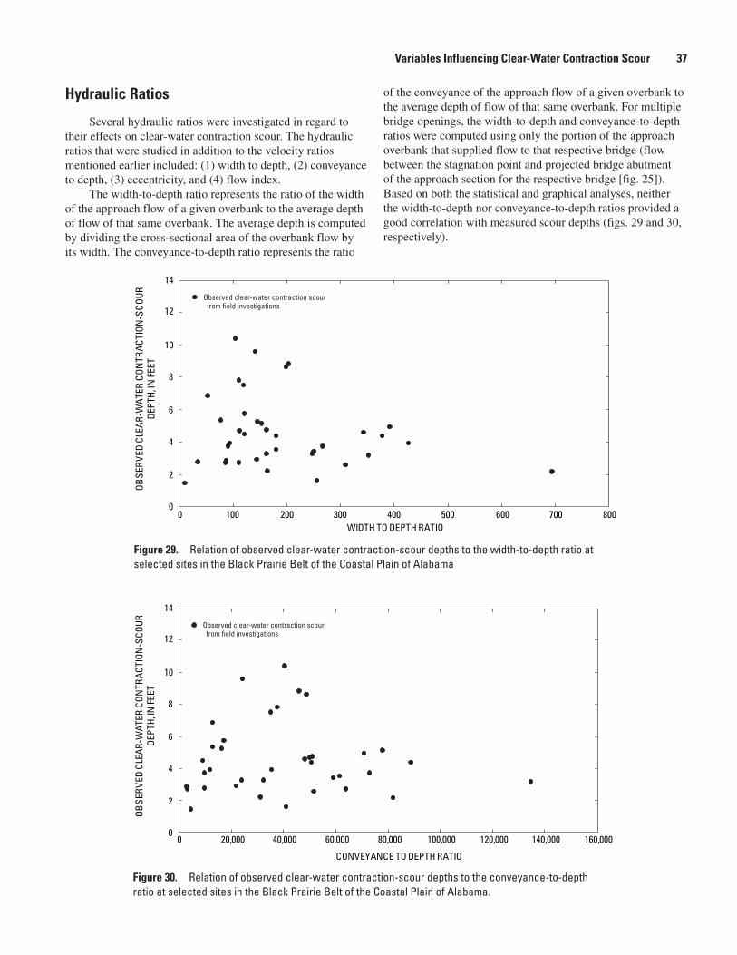
Variables Influencing Clear-Water Contraction Scour 37
Hydraulic Ratios
Several hydraulic ratios were investigated in regard to their effects on clear-water contraction scour. The hydraulic ratios that were studied in addition to the velocity ratios mentioned earlier included: (1) width to depth, (2) conveyance to depth, (3) eccentricity, and (4) flow index.
The width-to-depth ratio represents the ratio of the width of the approach flow of a given overbank to the average depth of flow of that same overbank. The average depth is computed by dividing the cross-sectional area of the overbank flow by its width. The conveyance-to-depth ratio represents the ratio
of the conveyance of the approach flow of a given overbank to the average depth of flow of that same overbank. For multiple bridge openings, the width-to-depth and conveyance-to-depth ratios were computed using only the portion of the approach overbank that supplied flow to that respective bridge (flow between the stagnation point and projected bridge abutment of the approach section for the respective bridge [fig. 25]). Based on both the statistical and graphical analyses, neither the width-to-depth nor conveyance-to-depth ratios provided a good correlation with measured scour depths (figs. 29 and 30, respectively).
Figure 29. Relation of observed clear-water contraction-scour depths to the width-to-depth ratio at selected sites in the Black Prairie Belt of the Coastal Plain of Alabama
Figure 30. Relation of observed clear-water contraction-scour depths to the conveyance-to-depth ratio at selected sites in the Black Prairie Belt of the Coastal Plain of Alabama.
0
2
4
6
8
10
12
14
OBSE
RVED
CLE
AR-W
ATER
CON
TRAC
TION
-SCO
URDE
PTH,
IN FE
ET
0 100 200 300 400 500 600 700 800WIDTH TO DEPTH RATIO
Observed clear-water contraction scour from field investigations
0 20,000 40,000 60,000 80,000 100,000 120,000 140,000 160,000
CONVEYANCE TO DEPTH RATIO
0
2
4
6
8
10
12
14
OBSE
RVED
CLE
AR-W
ATER
CON
TRAC
TION
-SCO
URDE
PTH,
IN FE
ET
Observed clear-water contraction scour from field investigations
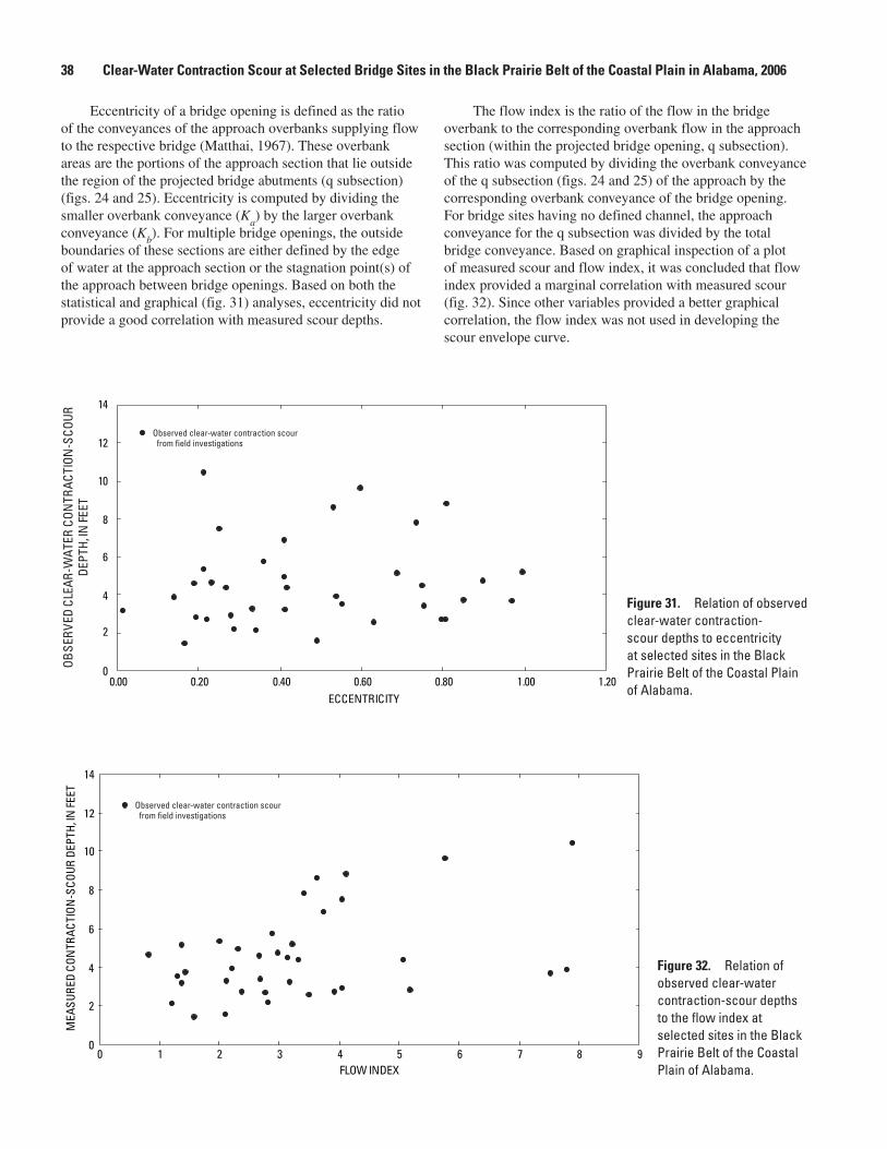
38 Clear-Water Contraction Scour at Selected Bridge Sites in the Black Prairie Belt of the Coastal Plain in Alabama, 2006
Eccentricity of a bridge opening is defined as the ratio of the conveyances of the approach overbanks supplying flow to the respective bridge (Matthai, 1967). These overbank areas are the portions of the approach section that lie outside the region of the projected bridge abutments (q subsection) (figs. 24 and 25). Eccentricity is computed by dividing the smaller overbank conveyance (K
a) by the larger overbank
conveyance (Kb). For multiple bridge openings, the outside
boundaries of these sections are either defined by the edge of water at the approach section or the stagnation point(s) of the approach between bridge openings. Based on both the statistical and graphical (fig. 31) analyses, eccentricity did not provide a good correlation with measured scour depths.
The flow index is the ratio of the flow in the bridge overbank to the corresponding overbank flow in the approach section (within the projected bridge opening, q subsection). This ratio was computed by dividing the overbank conveyance of the q subsection (figs. 24 and 25) of the approach by the corresponding overbank conveyance of the bridge opening. For bridge sites having no defined channel, the approach conveyance for the q subsection was divided by the total bridge conveyance. Based on graphical inspection of a plot of measured scour and flow index, it was concluded that flow index provided a marginal correlation with measured scour (fig. 32). Since other variables provided a better graphical correlation, the flow index was not used in developing the scour envelope curve.
Figure 31. Relation of observed clear-water contraction-scour depths to eccentricity at selected sites in the Black Prairie Belt of the Coastal Plain of Alabama.
Figure 32. Relation of observed clear-water contraction-scour depths to the flow index at selected sites in the Black Prairie Belt of the Coastal Plain of Alabama.
OBSE
RVED
CLE
AR-W
ATER
CON
TRAC
TION
-SCO
URDE
PTH,
IN FE
ET
Observed clear-water contraction scour from field investigations
0
2
4
6
8
10
12
14
0.00 0.20 0.40 0.60 0.80 1.00 1.20ECCENTRICITY
Observed clear-water contraction scour from field investigations
0
2
4
6
8
10
12
14
0 1 2 3 4 5 6 7 8 9FLOW INDEX
MEA
SURE
D CO
NTR
ACTI
ON-S
COUR
DEP
TH, IN
FEET
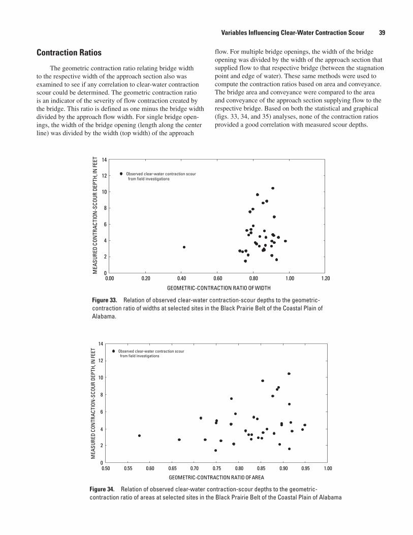
Variables Influencing Clear-Water Contraction Scour 39
Contraction Ratios
The geometric contraction ratio relating bridge width to the respective width of the approach section also was examined to see if any correlation to clear-water contraction scour could be determined. The geometric contraction ratio is an indicator of the severity of flow contraction created by the bridge. This ratio is defined as one minus the bridge width divided by the approach flow width. For single bridge open-ings, the width of the bridge opening (length along the center line) was divided by the width (top width) of the approach
flow. For multiple bridge openings, the width of the bridge opening was divided by the width of the approach section that supplied flow to that respective bridge (between the stagnation point and edge of water). These same methods were used to compute the contraction ratios based on area and conveyance. The bridge area and conveyance were compared to the area and conveyance of the approach section supplying flow to the respective bridge. Based on both the statistical and graphical (figs. 33, 34, and 35) analyses, none of the contraction ratios provided a good correlation with measured scour depths.
Figure 33. Relation of observed clear-water contraction-scour depths to the geometric-contraction ratio of widths at selected sites in the Black Prairie Belt of the Coastal Plain of Alabama.
Figure 34. Relation of observed clear-water contraction-scour depths to the geometric-contraction ratio of areas at selected sites in the Black Prairie Belt of the Coastal Plain of Alabama
Observed clear-water contraction scour from field investigations
0
2
4
6
8
10
12
14
MEA
SURE
D CO
NTR
ACTI
ON-S
COUR
DEP
TH, IN
FEET
0.00 0.20 0.40 0.60 0.80 1.00 1.20
GEOMETRIC-CONTRACTION RATIO OF WIDTH
Observed clear-water contraction scour from field investigations
0
2
4
6
8
10
12
14
MEA
SURE
D CO
NTR
ACTI
ON-S
COUR
DEP
TH, IN
FEET
0.50 0.55 0.60 0.65 0.70 0.75 0.80 0.85 0.90 0.95 1.00
GEOMETRIC-CONTRACTION RATIO OF AREA
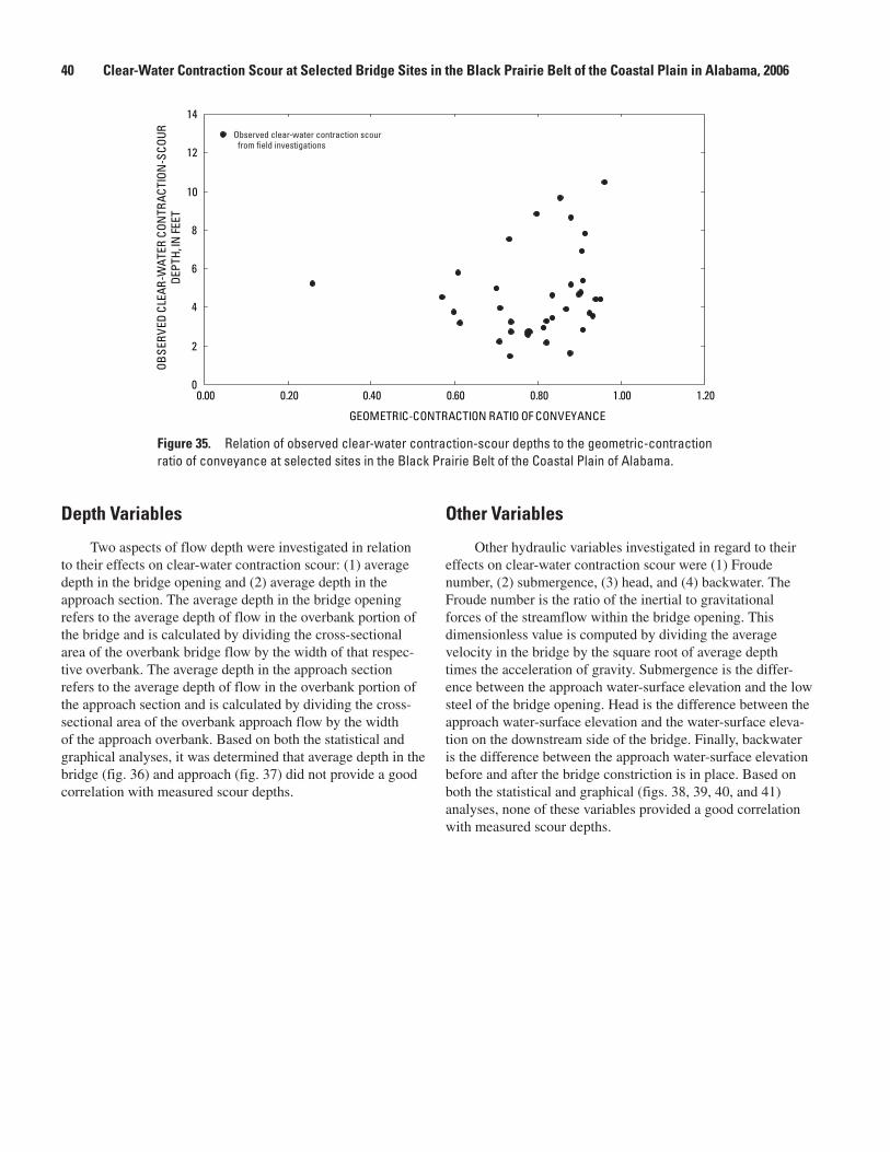
40 Clear-Water Contraction Scour at Selected Bridge Sites in the Black Prairie Belt of the Coastal Plain in Alabama, 2006
Depth Variables
Two aspects of flow depth were investigated in relation to their effects on clear-water contraction scour: (1) average depth in the bridge opening and (2) average depth in the approach section. The average depth in the bridge opening refers to the average depth of flow in the overbank portion of the bridge and is calculated by dividing the cross-sectional area of the overbank bridge flow by the width of that respec-tive overbank. The average depth in the approach section refers to the average depth of flow in the overbank portion of the approach section and is calculated by dividing the cross-sectional area of the overbank approach flow by the width of the approach overbank. Based on both the statistical and graphical analyses, it was determined that average depth in the bridge (fig. 36) and approach (fig. 37) did not provide a good correlation with measured scour depths.
Other Variables
Other hydraulic variables investigated in regard to their effects on clear-water contraction scour were (1) Froude number, (2) submergence, (3) head, and (4) backwater. The Froude number is the ratio of the inertial to gravitational forces of the streamflow within the bridge opening. This dimensionless value is computed by dividing the average velocity in the bridge by the square root of average depth times the acceleration of gravity. Submergence is the differ-ence between the approach water-surface elevation and the low steel of the bridge opening. Head is the difference between the approach water-surface elevation and the water-surface eleva-tion on the downstream side of the bridge. Finally, backwater is the difference between the approach water-surface elevation before and after the bridge constriction is in place. Based on both the statistical and graphical (figs. 38, 39, 40, and 41) analyses, none of these variables provided a good correlation with measured scour depths.
Figure 35. Relation of observed clear-water contraction-scour depths to the geometric-contraction ratio of conveyance at selected sites in the Black Prairie Belt of the Coastal Plain of Alabama.
Observed clear-water contraction scour from field investigations
0
2
4
6
8
10
12
14
0.00 0.20 0.40 0.60 0.80 1.00 1.20
GEOMETRIC-CONTRACTION RATIO OF CONVEYANCE
OBSE
RVED
CLE
AR-W
ATER
CON
TRAC
TION
-SCO
URDE
PTH,
IN FE
ET
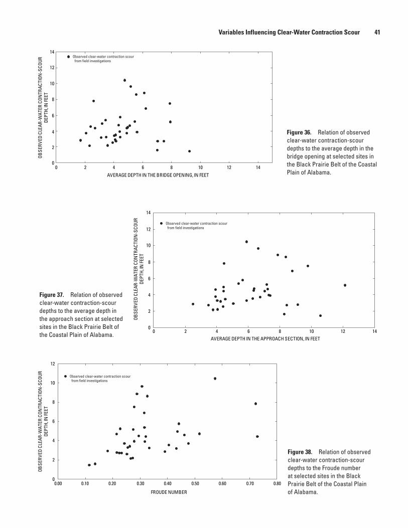
Variables Influencing Clear-Water Contraction Scour 41
Figure 36. Relation of observed clear-water contraction-scour depths to the average depth in the bridge opening at selected sites in the Black Prairie Belt of the Coastal Plain of Alabama.
Figure 37. Relation of observed clear-water contraction-scour depths to the average depth in the approach section at selected sites in the Black Prairie Belt of the Coastal Plain of Alabama.
Figure 38. Relation of observed clear-water contraction-scour depths to the Froude number at selected sites in the Black Prairie Belt of the Coastal Plain of Alabama.
0
2
4
6
8
10
12
14
OBSE
RVED
CLE
AR-W
ATER
CON
TRAC
TION
-SCO
URDE
PTH,
IN FE
ET
Observed clear-water contraction scour from field investigations
0 2 4 6 8 10 12 14
AVERAGE DEPTH IN THE BRIDGE OPENING, IN FEET
Observed clear-water contraction scour from field investigations
0
2
4
6
8
10
12
14
OBSE
RVED
CLE
AR-W
ATER
CON
TRAC
TION
-SCO
URDE
PTH,
IN FE
ET
0 2 4 6 8 10 12 14AVERAGE DEPTH IN THE APPROACH SECTION, IN FEET
Observed clear-water contraction scour from field investigations
0
2
4
6
8
10
12
OBSE
RVED
CLE
AR-W
ATER
CON
TRAC
TION
-SCO
URDE
PTH,
IN FE
ET
0.00 0.10 0.20 0.30 0.40 0.50 0.60 0.70 0.80
FROUDE NUMBER
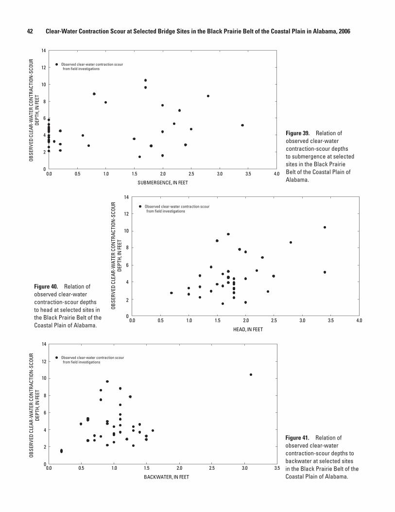
42 Clear-Water Contraction Scour at Selected Bridge Sites in the Black Prairie Belt of the Coastal Plain in Alabama, 2006
Figure 39. Relation of observed clear-water contraction-scour depths to submergence at selected sites in the Black Prairie Belt of the Coastal Plain of Alabama.
Figure 40. Relation of observed clear-water contraction-scour depths to head at selected sites in the Black Prairie Belt of the Coastal Plain of Alabama.
Figure 41. Relation of observed clear-water contraction-scour depths to backwater at selected sites in the Black Prairie Belt of the Coastal Plain of Alabama.
Observed clear-water contraction scour from field investigations
OBSE
RVED
CLE
AR-W
ATER
CON
TRAC
TION
-SCO
URDE
PTH,
IN FE
ET
0
2
4
6
8
10
12
14
0.0 0.5 1.0 1.5 2.0 2.5 3.0 3.5 4.0
SUBMERGENCE, IN FEET
Observed clear-water contraction scour from field investigations
OBSE
RVED
CLE
AR-W
ATER
CON
TRAC
TION
-SCO
URDE
PTH,
IN FE
ET
0
2
4
6
8
10
12
14
0.0 0.5 1.0 1.5 2.0 2.5 3.0 3.5 4.0
HEAD, IN FEET
Observed clear-water contraction scour from field investigations
OBSE
RVED
CLE
AR-W
ATER
CON
TRAC
TION
-SCO
URDE
PTH,
IN FE
ET
0
2
4
6
8
10
12
14
0.0 0.5 1.0 1.5 2.0 2.5 3.0 3.5
BACKWATER, IN FEET
Development of the Alabama Clear-Water Contraction Scour Envelope Curves 43
Development of the Alabama Clear-Water Contraction Scour Envelope Curves
Statistical analyses were performed to determine which geometric/hydraulic variable(s) could provide a good correla-tion to measured scour observed across the Black Prairie Belt. The minimum R2 selection method, used by the Statistical Analysis System (SAS), was used to evaluate the statistical significance of each possible explanatory variable (Freund and Littell, 1991). None of the variables tested provided a good statistical correlation (R2 > 0.8). Graphical methods were used to plot each of the variables against measured scour, and the resulting plots were visually inspected to see which ones would produce the most reasonable envelope curve(s). Enve-lope curves are curves that define the upper limit of observed scour throughout the range of collected data. Envelope curves developed with field data are useful tools for assessing reason-able ranges of scour depth in the Black Prairie Belt. After graphical inspection of all the potential explanatory variables, it was concluded that the channel-contraction ratio and the velocity index provided the best envelope curves. Envelope curves using the velocity index and the channel-contraction ratio as explanatory variables are shown in figures 42 and 43, respectively.
Application of the Alabama Contraction-Scour Envelope Curves
When assessing the clear-water contraction-scour depths using envelope curves presented in this report, both curves should be applied to site(s) of interest. These two envelope curves will often provide different estimates for the clear-water contraction-scour depth. Application of these envelope curves to the 25 bridge sites (37 hydraulic structures) used in this study has shown that the velocity index envelope provided the higher estimate of clear-water contraction scour for 18 out of 37 structures (51 percent). On average, the velocity index envelope estimated about 0.15 ft more scour depth than the channel-contraction envelope. After comparing the results of both envelopes, one should use the larger of the two estimated scour depths.
The channel-contraction ratio envelope curve is valid for channel-contraction ratios between 0.25 and 1.0, which roughly corresponds to scour depths between 2 and 13 ft. The velocity index envelope is valid for velocity indexes between 1 and 11, which roughly corresponds to scour depths between 4 and 11 ft. Both envelope curves should be used for sites that are located in the Black Prairie Belt of the Coastal Plain of Alabama.
When using these envelope curves, the potential error and limitations of these curves should be considered. These
envelope curves were developed using modeled hydraulic data that only estimate the true hydraulic conditions that created the observed scour. It is probable that errors exist within the hydraulic estimates, thus introducing error within the envelope curves. The clear-water contraction-scour envelope curves were developed using hydraulic data estimated with the hypothetical 50-year flood flow. Although it is unlikely that all study sites experienced this flow magnitude, there is evidence to suggest that most sites experienced flows equaling or exceeding this flow magnitude. The envelope curves should not be used to assess scour for extreme events larger than the 100-year recurrence interval flood. Finally, engineers should be aware that deeper scour in this region could be possible and, therefore, warrant the application of a safety factor.
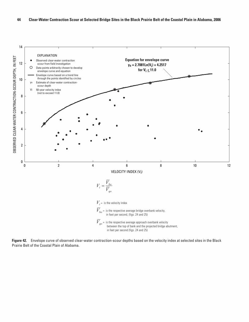
44 Clear-Water Contraction Scour at Selected Bridge Sites in the Black Prairie Belt of the Coastal Plain in Alabama, 2006
Figure 42. Envelope curve of observed clear-water contraction-scour depths based on the velocity index at selected sites in the Black Prairie Belt of the Coastal Plain of Alabama.
qo
boi V
VV
iV = is the velocity index
boV = is the respective average bridge overbank velocity, in feet per second, (figs. 24 and 25)
qoV = is the respective average approach overbank velocity between the top of bank and the projected bridge abutment, in feet per second (figs. 24 and 25)
0
2
4
6
8
10
12
14
0 2 4 6 8 10 12
VELOCITY INDEX (Vi)
OBSE
RVED
CLE
AR-W
ATER
CON
TRAC
TION
-SCO
UR D
EPTH
, IN
FEE
T EXPLANATIONObserved clear-water contraction scour from field investigationData points arbitrarily chosen to develop envelope curve and equationEnvelope curve based on a trend line through the points identified by circlesEstimate of clear-water contraction- scour depth50-year velocity index (not to exceed 11.0)
ys
Vi
Equation for envelope curveys = 2.7081Ln(Vi) + 4.2517
for Vi < 11.0
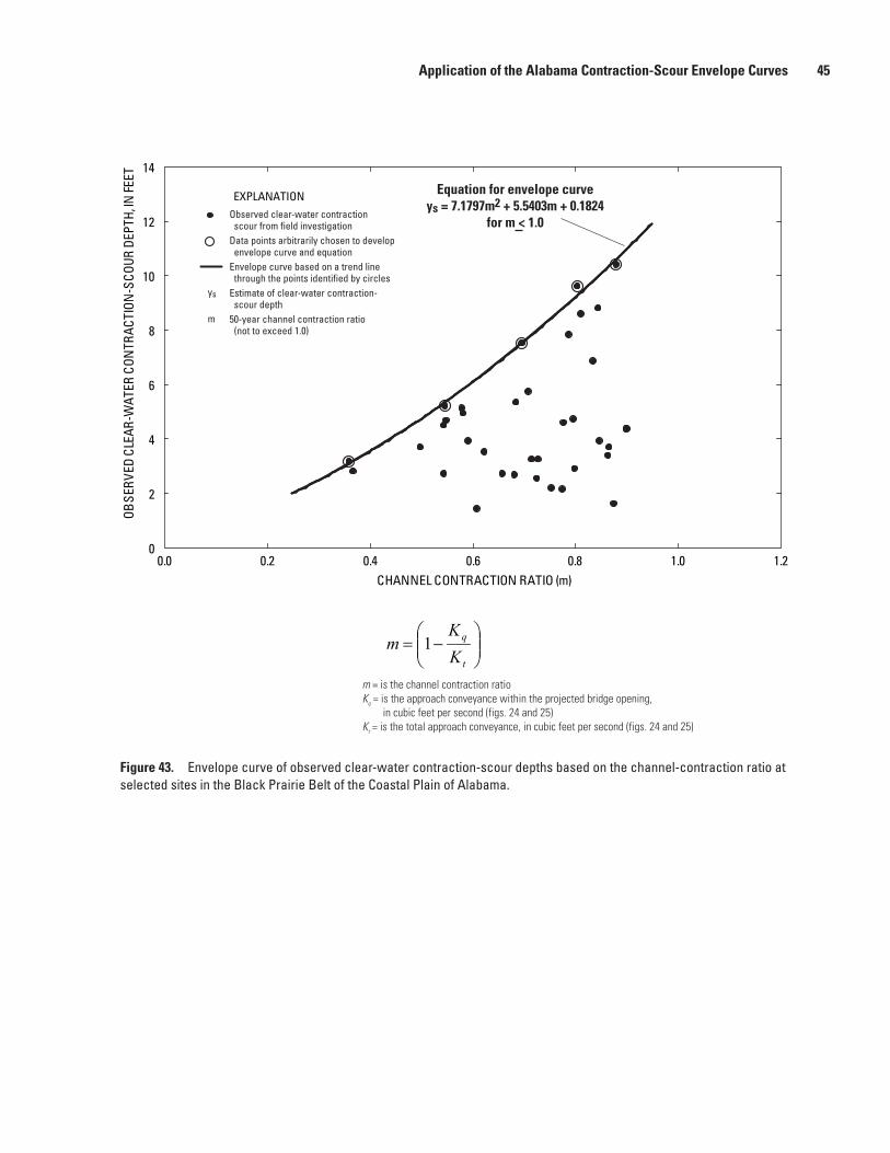
Application of the Alabama Contraction-Scour Envelope Curves 45
Figure 43. Envelope curve of observed clear-water contraction-scour depths based on the channel-contraction ratio at selected sites in the Black Prairie Belt of the Coastal Plain of Alabama.
t
q
KK
m 1
m = is the channel contraction ratio Kq = is the approach conveyance within the projected bridge opening, in cubic feet per second (figs. 24 and 25) Kt = is the total approach conveyance, in cubic feet per second (figs. 24 and 25)
0
2
4
6
8
10
12
14
0.0 0.2 0.4 0.6 0.8 1.0 1.2CHANNEL CONTRACTION RATIO (m)
OBSE
RVED
CLE
AR-W
ATER
CON
TRAC
TION
-SCO
UR D
EPTH
, IN FE
ET
EXPLANATIONObserved clear-water contraction scour from field investigationData points arbitrarily chosen to develop envelope curve and equationEnvelope curve based on a trend line through the points identified by circlesEstimate of clear-water contraction- scour depth50-year channel contraction ratio (not to exceed 1.0)
ys
m
Equation for envelope curveys = 7.1797m2 + 5.5403m + 0.1824
for m < 1.0
46 Clear-Water Contraction Scour at Selected Bridge Sites in the Black Prairie Belt of the Coastal Plain in Alabama, 2006
SummaryThe U.S. Geological Survey, in cooperation with the
Alabama Department of Transportation, made observations of clear-water contraction scour at 25 bridge sites (37 hydraulic structures) in the Black Prairie Belt of the Coastal Plain of Alabama. Observed scour depths ranged from 1.4 to 10.4 feet. Theoretical clear-water contraction-scour depths were com-puted for each bridge using HEC-18 methodology and were compared with observed scour. This comparison showed that theoretical scour depths, in general, exceeded the observed-scour depths by about 475 percent.
Variables determined to be important in developing scour within laboratory studies along with several other hydraulic variables were investigated to understand their influence within the Alabama field data. The variables investigated included grain size, velocity variables, channel-contraction ratio, hydraulic ratios, contraction ratios, depth variables, and other variables. None of the variables tested provided a good statistical correlation (R2 > 0.8). Graphical methods were used to plot each of the variables against measured scour, and the resulting plots were visually inspected to determine which ones would produce the most reasonable envelope curve(s). These envelope curves define the upper limit of observed scour throughout the range of data collected.
The strongest explanatory variables for clear-water contraction scour were channel-contraction ratio and velocity index. Envelope curves were developed relating both of these explanatory variables to observed scour. When assessing the clear-water contraction-scour depths using the envelope curves presented in this report, both curves should be applied to site(s) of interest. After comparing the results of both curves, the larger of the two estimated scour depths should be used. When assessing the results of the envelope curves the potential error and limitations of these curves should be considered. The clear-water contraction-scour envelope curves were developed using modeled hydraulic data estimated with the hypothetical 50-year flood flow. The envelope curves should not be used to assess scour for extreme events larger than the 100-year recurrence interval flood. It also should be considered that deeper scour in this region could be possible and may warrant the application of a safety factor. These envelope curves provide a useful tool for assessing reasonable ranges of scour depth in the Black Prairie Belt of Alabama.
References Cited
Alabama Coastal Hazards Assessment, 2001, Alabama hazards identification, accessed January 12, 2007, at http://www.warnercnr.colostate.edu/avprojects/00proj/hurr_haz/web_docs/htm/hazid.htm#top
Atkins, J.B., 1996, Magnitude and frequency of floods in Ala-bama: U.S. Geological Survey Water-Resources Investiga-tions Report 95–4199, 234 p.
Barnes, H.H., Jr., and Somers, W.P., 1961, Floods of February-March 1961 in the Southeastern States: U.S. Geological Survey Circular 452, 21 p.
Bedient, P.B., and Huber, W.C., 1988, Hydrology and analysis: Reading, MA, Addison-Wesley Publishing Company, 650 p.
Benedict, S.T., 2003, Clear-water abutment and contrac-tion scour in the Coastal Plain and Piedmont Provinces of South Carolina, 1996–99: U.S. Geological Survey Water-Resources Investigations Report 2003–4064, 137 p.
Benedict, S.T., and Caldwell, A.W., 2005, Development and evaluation of clear-water pier and contraction scour enve-lope curves in the Coastal Plain and Piedmont Provinces of South Carolina: U.S. Geological Survey Scientific Investi-gations Report 2005–5289, 98 p.
Brabets, T.P., 1995, Application of surface geophysical tech-niques in a study of the geomorphology of the lower Copper River, Alaska: U.S. Geological Survey Water-Resources Investigations Report 94–4165, 47 p.
Briaud, J.-L., Chen, H.-C., Li, Y., Nurtjahyo, P., and Wang, J., 2004, Pier and contraction scour in cohesive soils: Washing-ton, DC, Transportation Research Board, National Coopera-tive Highway Research Program Report 516, 118 p.
Crim, S.H., Jr., Parker, Frazier, Jr., Melville, J.G., Curry, J.E., and Güven, Oktay, 2003, Erosion characteristics of Ala-bama soils obtained with the Erosion Function Apparatus and correlations with classification properties: Auburn University—Highway Research Center Report 930–490, 27 p.
Daugherty, R.L., and Ingersoll, A.C., 1954, Fluid mechanics with engineering applications: New York, McGraw-Hill Book Company, Inc., 472 p.
Dongol, D.M.S., 1993, Local scour at bridge abutments: New Zealand, University of Auckland, School of Engineering Report No. 544, 410 p.
Edelen, G.W., Jr., Wilson, K.V., Harkins, J.R., Miller, J.F., and Chin, E.H., 1986, Floods of April 1979, Mississippi, Alabama, and Georgia: U.S. Geological Survey Professional Paper 1319, 212 p.
Fenneman, N.M., 1938, Physiography of the Eastern United States: New York, McGraw-Hill Book Company, 691 p.
Fischer, E.E., 1995, Contraction scour at a bridge over Wolf Creek, Iowa, in Water Resources Research: San Antonio, TX, American Society of Civil Engineers, p. 430–434.
References Cited 47
Fortier, Samuel, and Scobey, F.C., 1926, Permissible canal velocities: Transactions of the American Society of Civil Engineers, v. 89, no. 1588, p. 940–984.
Freund, R.J., and Littell, R.C., 1991, SAS System for Regres-sion (2nd ed.): Cary, NC, SAS Institute Inc., 210 p.
Government Performance Project, 2005, Alabama— Infra-structure— Maintenance, accessed September 27, 2006, at http://results.gpponline.org/StateCategoryCriteria.aspx?id=93&relatedid=4#12
Hedgecock, T.S., 2003, Simulation of flooding on Pea River and Whitewater Creek in the vicinity of the proposed Elba Bypass at Elba, Alabama: U.S. Geological Survey Water-Resources Investigations Report 2002–4258, 35 p.
Holnbeck, S.R., Parrett, C., and Tillinger, T.N., 1993, Bridge scour and change in contracted section, Razor Creek, MT, in Shen, H.W., Su, T.H., and Weng, F., eds., Hydraulic engineering 1993: San Francisco, CA, American Society of Civil Engineers, p. 2249–2254.
Jordan, P.R., and Combs, L.J., eds., 1996, Summary of floods in the United States during 1990 and 1991: U.S. Geological Survey Water-Supply Paper 2474, 254 p.
Keown, M.P., Oswalt, N.R., Perry, E.B., and Dordeau, E.A., Jr., 1977, Literature survey and preliminary evaluation of streambank protection methods: U.S. Army Corps of Engi-neers, Waterways Experiment Station, Technical Report H–79–9.
Lagasse, P.F., Schall, J.D., Johnson, F., Richardson, E.V., Richardson, J.R., and Chang, F., 1991, Stream stability at highway structures: U.S. Department of Transportation Federal Highway Administration Hydraulic Engineering Circular No. 20, Publication FHWA–IP–90–014, 195 p.
Laursen, E.M., 1963, Scour at bridge crossings: Journal Hydraulic Division, American Society of Engineers, v. 89, no. HY3.
Leonards, G.A., 1950, Description and identification of soils—The engineering significance of descriptive soil ter-minology: West Lafayette, IN, Purdue University, 15 p.
Matthai, H.F., 1967, Measurement of peak discharge at width contractions by indirect methods—Applications of Hydrau-lics, Techniques of Water-Resources Investigations of the U.S. Geological Survey, book 3, chap. A4, 44 p.
Methods, Haestad, Dyhouse, Gary, Hatchett, Jennifer, and Benn, Jeremy, 2003, Floodplain modeling using HEC-RAS: Waterbury, CT, Haested Press, 696 p.
Miller, J.A., 1990, Ground water atlas of the United States— Segment 6, Alabama, Florida, Georgia, and South Carolina: U.S. Geological Survey Hydrologic Investigations Atlas 730–G, 28 p.
Moody, D.W., Chase, E.B., and Aronson, D.A., comps., 1986, National water summary 1985—Hydrologic events and surface-water resources: U.S. Geological Survey Water-Supply Paper 2300, 506 p.
Mueller, D.S., and Wagner C.R., 2005, Field observations and evaluations of streambed scour at bridges: U.S. Department of Transportation Federal Highway Administration FHWA–RD–03–052, 122 p.
Multi-Resolution Land Characteristics Consortium, 2006: National Land Cover Database 2001, accessed July 19, 2006, at http://www.mrlc.gov/mrlc2k_nlcd.asp
National Resource Conservation Service, U. S. Department of Agriculture, 2006, U.S. General Soil Map (STATSGO) for Alabama, accessed January 17, 2006, at http://soildatamart.nrcs.usda.gov
National Transportation Safety Board, 1971, Highway acci-dent report—Collapse of U.S. 35 highway bridge, Point Pleasant, West Virginia, December 15, 1967: NTSB no. HAR–71/01, accessed September 27, 2006, at http://www.ntsb.gov/publictn/1971/HAR7101.htm
National Transportation Safety Board, 1988, Highway acci-dent report—Collapse of New York thruway (I–90) bridge, Schoharir Creek, near Amsterdam, New York, April 5, 1987: NTBS No. HAR–88/02, accessed September 27, 2006, at http://www.ntsb.gov/publictn/1988/HAR8802.htm
National Transportation Safety Board, 1990, Highway accident report—Collapse of the northbound U.S. Route 51 bridge spans over the Hatchie River near Covington, Tennessee, April 1, 1989: NTBS No. HAR-90/01, accessed September 27, 2006, at http://www.ntsb.gov/publictn/1990/HAR9001.htm
Neill, C.R., ed., 1973, Guide to bridge hydraulics: Toronto, Canada, University of Toronto Press, 191 p.
Norman, V.W., 1975, Scour at selected bridge sites in Alaska: U.S. Geological Survey Water-Resources Investigations Report 75–32, 171 p.
Paulson, R.W., Chase, E.B., Roberts, R.S., and Moody, D.W., compilers, 1991, National water summary, 1988–89 —Hydrologic events and floods and droughts: U.S. Geological Survey Water-Supply Paper 2375, 591 p.
Pearman, J.L., Stamey, T.C., Hess, G.W., and Nelson, G.H., Jr., 1991, Floods of February and March 1990 in Alabama, Georgia, and Florida: U.S. Geological Survey Water-Resources Investigations Report 91–4089, 44 p.
Perry, C.A., Aldridge, B.N., and Ross, H.C., 2001 Summary of significant floods in the United States, Puerto Rico, and the Virgin Islands, 1970 through 1989: U.S. Geological Survey Water-Supply Paper 2502, 598 p.
48 Clear-Water Contraction Scour at Selected Bridge Sites in the Black Prairie Belt of the Coastal Plain in Alabama, 2006
Rankin, H.T., 1974, Black Belt Prairie—Montgomery County, Alabama, and vicinity: Alabama Agricultural Experi-ments Station, accessed December 15, 2006, at http://www.ag.auburn.edu/ aaes/communications/bulletins/bull454/
Richardson, E.V., and Davis, S.R., 2001, Evaluating scour at bridges: U.S. Department of Transportation Federal High-way Administration Hydraulic Engi neering Circular No. 18, Federal Highway Administration Publication No. FHWA NHI–01–001, 378 p.
Richardson, E.V., Harrison, L.J., and Davis, S.R., 1991, Evalu-ating scour at bridges: Federal Highway Administration Hydraulic Engineering Circular No. 18, Federal Highway Administration Publication No. FHWA–IP–90–017, 105 p.
Richardson, E.V., Simons, D.B., and Julien, P.Y., 1990, Highways in the river environment— participant notebook: Federal Highway Administration FHWA–HI–90–016, 494 p.
Road Information Program, 2002, Showing their age: The Nation’s bridges at 40 —Strategies to improve the condition of our bridges and keep them in good shape, accessed September 27, 2006, at http://www.rebuildca.org/pdfs/BridgesReportMay2002.PDF
Rostvedt, J.O., 1961, Summary of floods in the United States during 1961: U.S. Geological Survey Water-Supply Paper 1810, 123 p.
Rostvedt, J.O., and others, 1970, Summary of floods in the United States during 1964: U.S. Geological Survey Water-Supply Paper 1840–C, 124 p.
Shearman, J.O., 1990, User’s manual for WSPRO—A com-puter model for water surface profile computations: Federal Highway Administration Report no. FHWA–IP–89–027, 175 p.
U.S. Department of Transportation Federal Highway Admin-istration, 2003, Scour screening/evaluations by state – total highway bridges as of April 15, 2003, accessed May 24, 2004, at http://www.fhwa.dot.gov/engineering/hydraulics/policymemo/ scour.cfm
U.S. Department of Transportation Federal Highway Admin-istration, 2006, Annual vehicle-miles Federal-aid highway travel-2005, accessed December 12, 2006, at http://www.fhwa.dot.gov/policy/ohim/hs05/pdf/vm3.pdf
U.S. Geological Survey, 1953, Floods of March–April 1951 in Alabama and adjacent states: U.S. Geological Survey Water-Supply Paper 1227–A, 134 p.
U.S. Geological Survey, 1992, National Land Cover Dataset 1992, accessed December 1, 2005, at http://landcover.usgs.gov/natllandcover.php
U.S. Geological Survey, 2006, National Elevation Dataset, accessed December 29, 2006, at http://ned.usgs.gov/.
Vanoni, V.A., ed., 1975, Sedimentation engineering: New York, American Society of Civil Engineers, 745 p.
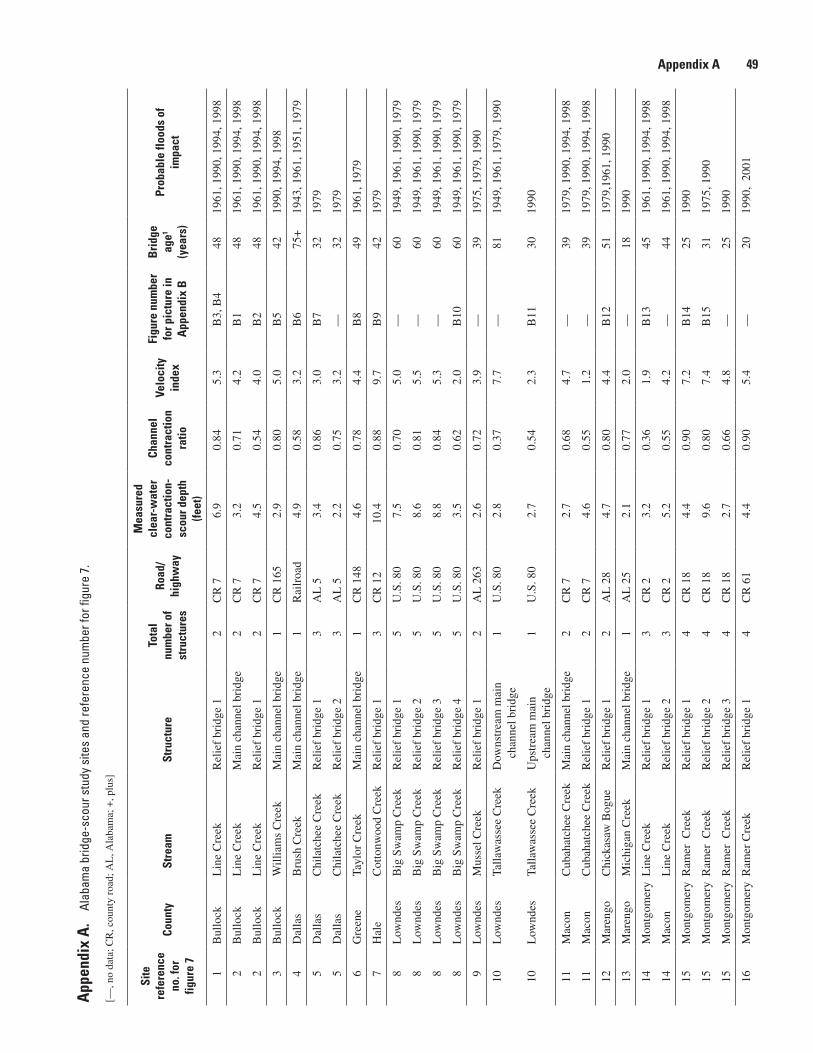
Appendix A 49A
ppen
dix
A.
Alab
ama
brid
ge-s
cour
stu
dy s
ites
and
refe
renc
e nu
mbe
r for
figu
re 7
. — C
ontin
ued
[—, n
o da
ta; C
R, c
ount
y ro
ad; A
L, A
laba
ma;
+, p
lus]
Site
re
fere
nce
no. f
or
figur
e 7
Coun
tySt
ream
Stru
ctur
eTo
tal
num
ber o
f st
ruct
ures
Road
/ hi
ghw
ay
Mea
sure
d
clea
r-w
ater
co
ntra
ctio
n-
scou
r dep
th(fe
et)
Chan
nel
cont
ract
ion
ratio
Velo
city
in
dex
Figu
re n
umbe
r fo
r pic
ture
in
App
endi
x B
Bri
dge
age1
(yea
rs)
Prob
able
floo
ds o
f im
pact
1B
ullo
ckL
ine
Cre
ekR
elie
f br
idge
12
CR
76.
90.
845.
3B
3, B
448
1961
, 199
0, 1
994,
199
8
2B
ullo
ckL
ine
Cre
ekM
ain
chan
nel b
ridg
e2
CR
73.
20.
714.
2B
148
1961
, 199
0, 1
994,
199
8
2B
ullo
ckL
ine
Cre
ekR
elie
f br
idge
12
CR
74.
50.
544.
0B
248
1961
, 199
0, 1
994,
199
8
3B
ullo
ckW
illia
ms
Cre
ekM
ain
chan
nel b
ridg
e1
CR
165
2.9
0.80
5.0
B5
4219
90, 1
994,
199
8
4D
alla
sB
rush
Cre
ekM
ain
chan
nel b
ridg
e1
Rai
lroa
d4.
90.
583.
2B
675
+19
43, 1
961,
195
1, 1
979
5D
alla
sC
hila
tche
e C
reek
Rel
ief
brid
ge 1
3A
L 5
3.4
0.86
3.0
B7
3219
79
5D
alla
sC
hila
tche
e C
reek
Rel
ief
brid
ge 2
3A
L 5
2.2
0.75
3.2
—32
1979
6G
reen
eTa
ylor
Cre
ekM
ain
chan
nel b
ridg
e1
CR
148
4.6
0.78
4.4
B8
4919
61, 1
979
7H
ale
Cot
tonw
ood
Cre
ekR
elie
f br
idge
13
CR
12
10.4
0.88
9.7
B9
4219
79
8L
ownd
esB
ig S
wam
p C
reek
Rel
ief
brid
ge 1
5U
.S. 8
07.
50.
705.
0—
6019
49, 1
961,
199
0, 1
979
8L
ownd
esB
ig S
wam
p C
reek
Rel
ief
brid
ge 2
5U
.S. 8
08.
60.
815.
5—
6019
49, 1
961,
199
0, 1
979
8L
ownd
esB
ig S
wam
p C
reek
Rel
ief
brid
ge 3
5U
.S. 8
08.
80.
845.
3—
6019
49, 1
961,
199
0, 1
979
8L
ownd
esB
ig S
wam
p C
reek
Rel
ief
brid
ge 4
5U
.S. 8
03.
50.
622.
0B
1060
1949
, 196
1, 1
990,
197
9
9L
ownd
esM
usse
l Cre
ekR
elie
f br
idge
12
AL
263
2.6
0.72
3.9
—39
1975
, 197
9, 1
990
10L
ownd
esTa
llaw
asse
e C
reek
Dow
nstr
eam
mai
n ch
anne
l bri
dge
1U
.S. 8
02.
80.
377.
7—
8119
49, 1
961,
197
9, 1
990
10L
ownd
esTa
llaw
asse
e C
reek
Ups
trea
m m
ain
chan
nel b
ridg
e1
U.S
. 80
2.7
0.54
2.3
B11
3019
90
11M
acon
Cub
ahat
chee
Cre
ekM
ain
chan
nel b
ridg
e2
CR
72.
70.
684.
7—
3919
79, 1
990,
199
4, 1
998
11M
acon
Cub
ahat
chee
Cre
ekR
elie
f br
idge
12
CR
74.
60.
551.
2—
3919
79, 1
990,
199
4, 1
998
12M
aren
goC
hick
asaw
Bog
ueR
elie
f br
idge
12
AL
28
4.7
0.80
4.4
B12
5119
79,1
961,
199
0
13M
aren
goM
ichi
gan
Cre
ekM
ain
chan
nel b
ridg
e1
AL
25
2.1
0.77
2.0
—18
1990
14M
ontg
omer
yL
ine
Cre
ekR
elie
f br
idge
13
CR
23.
20.
361.
9B
1345
1961
, 199
0, 1
994,
199
8
14M
acon
Lin
e C
reek
Rel
ief
brid
ge 2
3C
R 2
5.2
0.55
4.2
—44
1961
, 199
0, 1
994,
199
8
15M
ontg
omer
yR
amer
Cre
ekR
elie
f br
idge
14
CR
18
4.4
0.90
7.2
B14
2519
90
15M
ontg
omer
yR
amer
Cre
ekR
elie
f br
idge
24
CR
18
9.6
0.80
7.4
B15
3119
75, 1
990
15M
ontg
omer
yR
amer
Cre
ekR
elie
f br
idge
34
CR
18
2.7
0.66
4.8
—25
1990
16M
ontg
omer
yR
amer
Cre
ekR
elie
f br
idge
14
CR
61
4.4
0.90
5.4
—20
1990
, 20
01
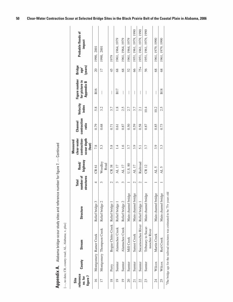
50 Clear-Water Contraction Scour at Selected Bridge Sites in the Black Prairie Belt of the Coastal Plain in Alabama, 2006
App
endi
x A
. Al
abam
a br
idge
-sco
ur s
tudy
site
s an
d re
fere
nce
num
ber f
or fi
gure
7. —
Con
tinue
d
[—, n
o da
ta; C
R, c
ount
y ro
ad; A
L, A
laba
ma;
+, p
lus]
Site
re
fere
nce
no. f
or
figur
e 7
Coun
tySt
ream
Stru
ctur
eTo
tal
num
ber o
f st
ruct
ures
Road
/ hi
ghw
ay
Mea
sure
d
clea
r-w
ater
co
ntra
ctio
n-
scou
r dep
th(fe
et)
Chan
nel
cont
ract
ion
ratio
Velo
city
in
dex
Figu
re n
umbe
r fo
r pic
ture
in
App
endi
x B
Bri
dge
age1
(yea
rs)
Prob
able
floo
ds o
f im
pact
16M
ontg
omer
yR
amer
Cre
ekR
elie
f br
idge
34
CR
61
7.8
0.79
5.8
B16
2019
90,
2001
17M
ontg
omer
yT
hom
pson
Cre
ekR
elie
f br
idge
23
Woo
dley
R
oad
5.3
0.68
3.2
—17
1990
, 20
01
18Pe
rry
Bog
ue C
hitto
Cre
ekR
elie
f br
idge
12
CR
38
5.8
0.71
3.7
—45
1979
19Su
mte
rA
lam
uche
e C
reek
Rel
ief
brid
ge 1
3A
L 1
71.
40.
611.
8B
1768
1961
, 196
4, 1
979
19Su
mte
rA
lam
uche
e C
reek
Rel
ief
brid
ge 2
3A
L 1
71.
60.
872.
5—
6819
61, 1
964,
197
9
20Su
mte
rM
ill C
reek
Mai
n ch
anne
l bri
dge
1U
.S. 8
03.
70.
502.
7—
5219
61, 1
964,
197
9
21Su
mte
rSa
nusi
Cre
ekM
ain
chan
nel b
ridg
e2
AL
17
3.9
0.59
3.7
—66
1951
, 196
1, 1
979,
199
0
22Su
mte
rSu
carn
ooch
ee R
iver
Rel
ief
brid
ge 1
2R
ailr
oad
5.1
0.58
2.1
—75
+19
51, 1
961,
197
9, 1
990
23Su
mte
rT
ribu
tary
to S
ucar
-no
oche
e R
iver
Mai
n ch
anne
l bri
dge
1C
R 1
23.
70.
8710
.4—
5619
51, 1
961,
197
9, 1
990
24W
ilcox
Mar
tin C
reek
Mai
n ch
anne
l bri
dge
1A
L 5
3.9
0.85
10.2
—68
1961
, 197
9, 1
990
25W
ilcox
Red
Cre
ekM
ain
chan
nel b
ridg
e1
AL
53.
30.
732.
5B
1868
1961
, 197
9, 1
990
1 The
bri
dge
age
for
the
railr
oad
stru
ctur
es w
as e
stim
ated
to b
e 75
+ y
ears
old
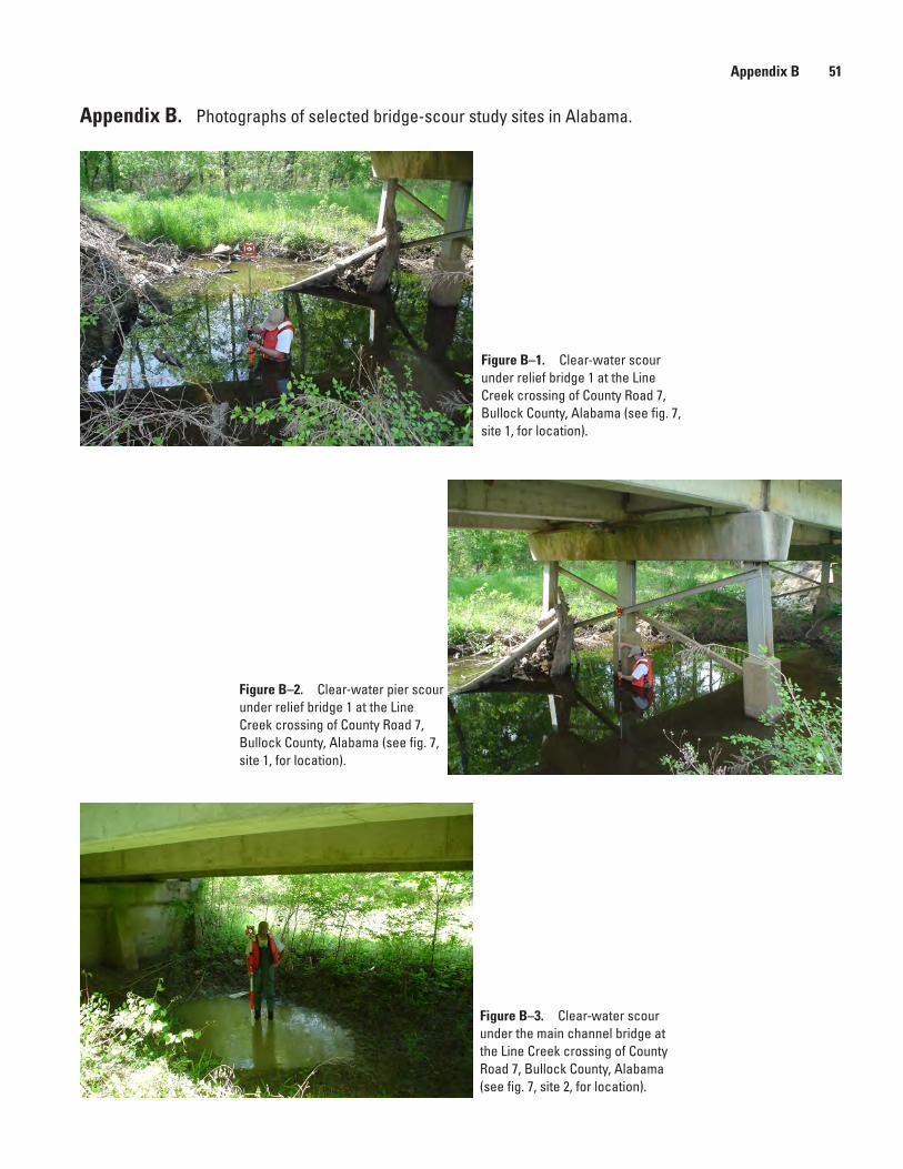
Appendix B 51
Appendix B. Photographs of selected bridge-scour study sites in Alabama.
Figure B–1. Clear-water scour under relief bridge 1 at the Line Creek crossing of County Road 7, Bullock County, Alabama (see fig. 7, site 1, for location).
Figure B–2. Clear-water pier scour under relief bridge 1 at the Line Creek crossing of County Road 7, Bullock County, Alabama (see fig. 7, site 1, for location).
Figure B–3. Clear-water scour under the main channel bridge at the Line Creek crossing of County Road 7, Bullock County, Alabama (see fig. 7, site 2, for location).
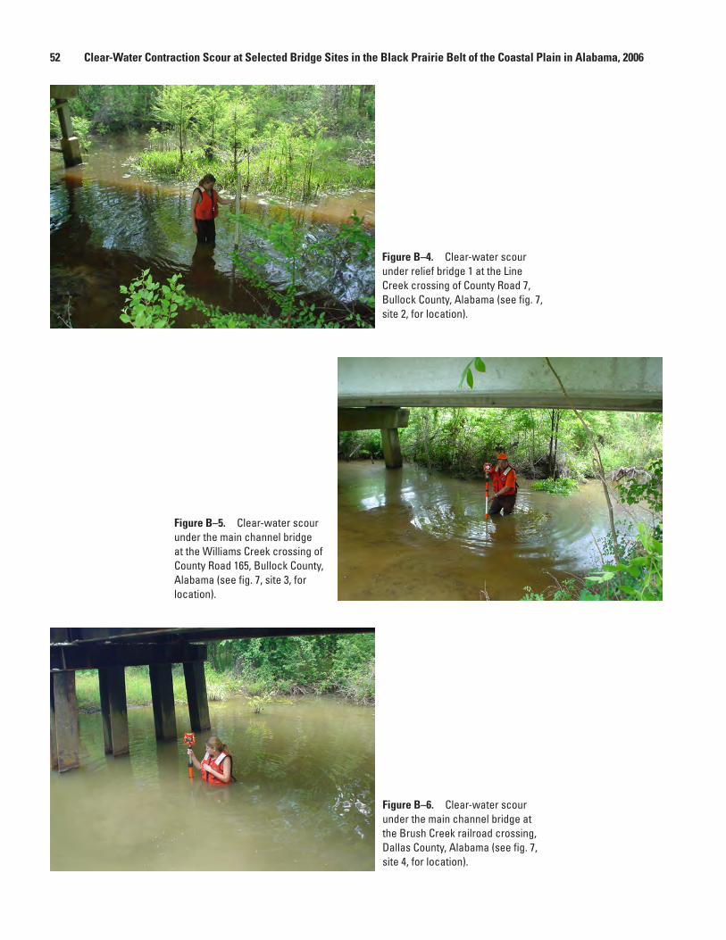
52 Clear-Water Contraction Scour at Selected Bridge Sites in the Black Prairie Belt of the Coastal Plain in Alabama, 2006
Figure B–4. Clear-water scour under relief bridge 1 at the Line Creek crossing of County Road 7, Bullock County, Alabama (see fig. 7, site 2, for location).
Figure B–5. Clear-water scour under the main channel bridge at the Williams Creek crossing of County Road 165, Bullock County, Alabama (see fig. 7, site 3, for location).
Figure B–6. Clear-water scour under the main channel bridge at the Brush Creek railroad crossing, Dallas County, Alabama (see fig. 7, site 4, for location).
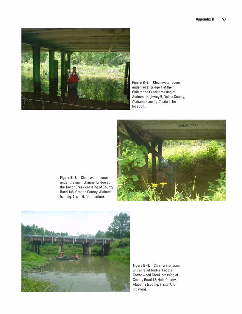
Appendix B 53
Figure B–7. Clear-water scour under relief bridge 1 at the Chilatchee Creek crossing of Alabama Highway 5, Dallas County, Alabama (see fig. 7, site 5, for location).
Figure B–8. Clear-water scour under the main channel bridge at the Taylor Creek crossing of County Road 148, Greene County, Alabama (see fig. 7, site 6, for location).
Figure B–9. Clear-water scour under relief bridge 1 at the Cottonwood Creek crossing of County Road 12, Hale County, Alabama (see fig. 7, site 7, for location).
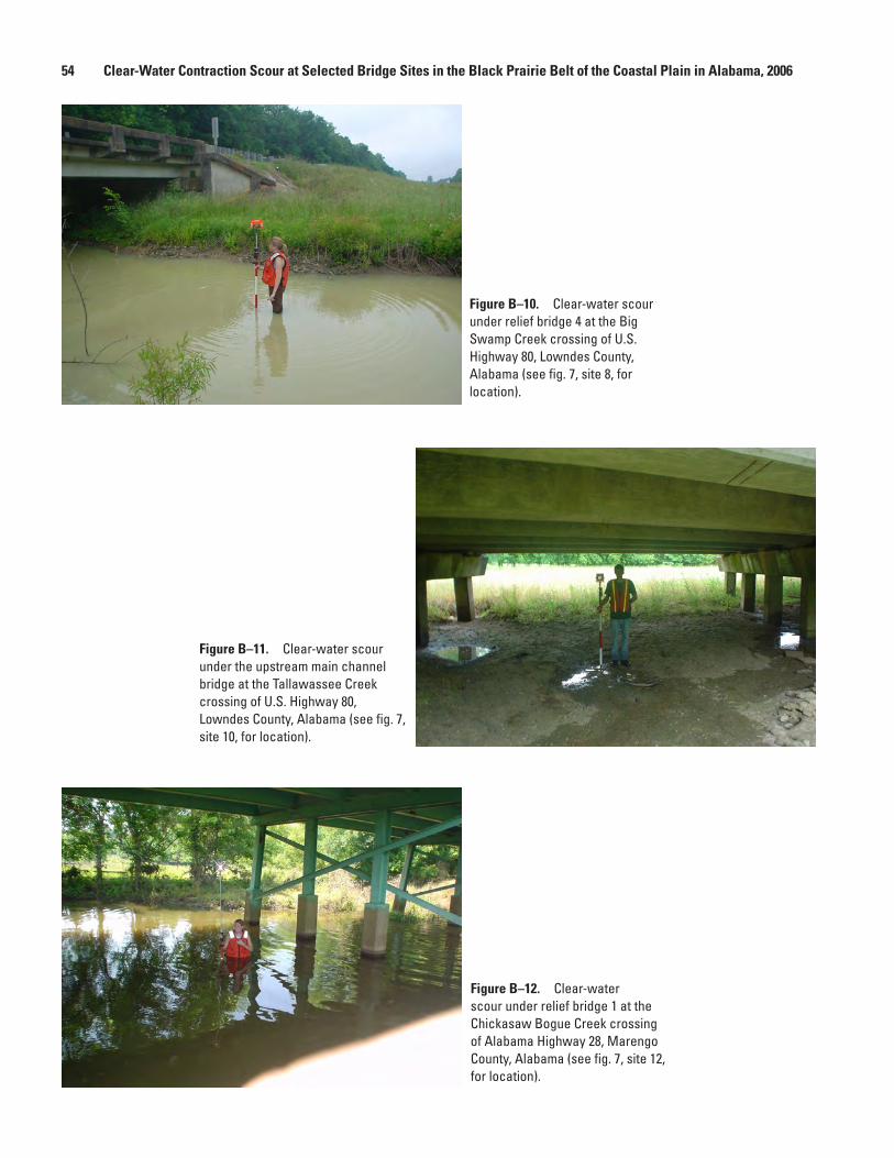
54 Clear-Water Contraction Scour at Selected Bridge Sites in the Black Prairie Belt of the Coastal Plain in Alabama, 2006
Figure B–10. Clear-water scour under relief bridge 4 at the Big Swamp Creek crossing of U.S. Highway 80, Lowndes County, Alabama (see fig. 7, site 8, for location).
Figure B–11. Clear-water scour under the upstream main channel bridge at the Tallawassee Creek crossing of U.S. Highway 80, Lowndes County, Alabama (see fig. 7, site 10, for location).
Figure B–12. Clear-water scour under relief bridge 1 at the Chickasaw Bogue Creek crossing of Alabama Highway 28, Marengo County, Alabama (see fig. 7, site 12, for location).
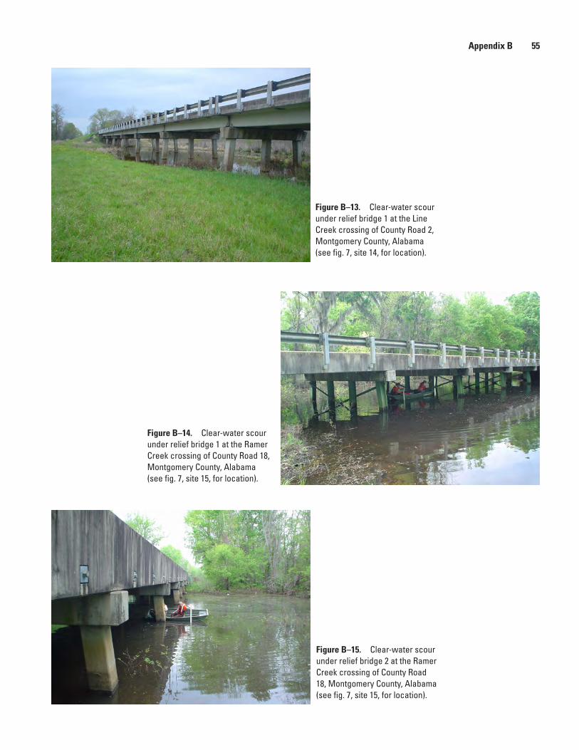
Appendix B 55
Figure B–13. Clear-water scour under relief bridge 1 at the Line Creek crossing of County Road 2, Montgomery County, Alabama (see fig. 7, site 14, for location).
Figure B–14. Clear-water scour under relief bridge 1 at the Ramer Creek crossing of County Road 18, Montgomery County, Alabama (see fig. 7, site 15, for location).
Figure B–15. Clear-water scour under relief bridge 2 at the Ramer Creek crossing of County Road 18, Montgomery County, Alabama (see fig. 7, site 15, for location).
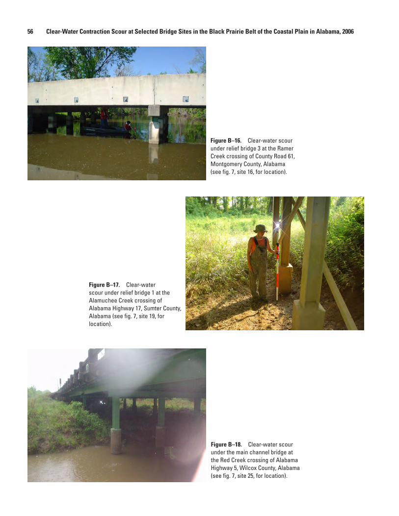
56 Clear-Water Contraction Scour at Selected Bridge Sites in the Black Prairie Belt of the Coastal Plain in Alabama, 2006
Figure B–16. Clear-water scour under relief bridge 3 at the Ramer Creek crossing of County Road 61, Montgomery County, Alabama (see fig. 7, site 16, for location).
Figure B–17. Clear-water scour under relief bridge 1 at the Alamuchee Creek crossing of Alabama Highway 17, Sumter County, Alabama (see fig. 7, site 19, for location).
Figure B–18. Clear-water scour under the main channel bridge at the Red Creek crossing of Alabama Highway 5, Wilcox County, Alabama (see fig. 7, site 25, for location).

Prepared by:USGS Publishing NetworkRaleigh Publishing Service Center3916 Sunset Ridge RoadRaleigh, NC 27607
For additional information regarding this publication, contact:DirectorUSGS Alabama Water Science Center75 TechnaCenter DriveMontgomery, AL 36117phone: 1-334-395-4120email: [email protected]
Or visit the Alabama Water Science Center website at:http://al.water.usgs.gov
This publication is available online at:http://pubs.water.usgs.gov/sir2007-5260

Printed on recycled paper
Lee and Hedgecock—Clear-W
ater Contraction Scour at Bridge Sites in the B
lack Prairie Belt in the Coastal Plain, A
labama, 2006—
Scientific Investigations Report 2007–5260
Printed on recycled paper