toe and bed scour lectures final 2008 - walter scott, jr ... and bed scour lectures... ·...

1

Estimating Scour

CIVE 510October 21st , 2008

2

Causes of Scour

3

Site Stability

4

Mass Failure• Downward movement of large and intact

masses of soil and rock• Occurs when weight on slope exceeds the

shear strength of bank material• Typically a result of water saturating a

slide-prone slope– Rapid draw down– Flood stage manipulation– Tidal effects– Seepage

5

Mass Failure• Rotational Slide

– Concave failure plane, typically on slopes ranging from 20-40 degrees

6

Mass Failure• Translational Slide

– Shallower slide, typically along well-defined plane

7

Site Stability

8

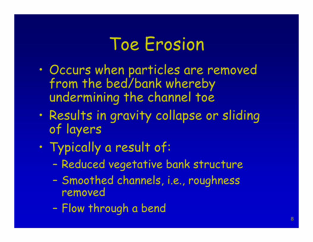
Toe Erosion• Occurs when particles are removed

from the bed/bank whereby undermining the channel toe

• Results in gravity collapse or sliding of layers

• Typically a result of:– Reduced vegetative bank structure– Smoothed channels, i.e., roughness

removed– Flow through a bend

9

Toe Erosion

10

Toe Erosion

11

Site Stability

12

Avulsion and Chute Cutoffs• Abrupt change in channel alignment

resulting in a new channel within the floodplain

• Typically caused by:– Concentrated overland flow– Headcutting and/or scouring within

floodplain– Manmade disturbances

• Chute cutoff – smaller scale than avulsion

13

Avulsion and Chute Cutoffs

14

Site Stability

15

Subsurface Entrainment• Piping – occurs when subsurface flow

transports soil particles resulting in the development of a tunnel.

• Tunnels reduce soil cohesion causing slippage and ultimately streambank erosion.

• Typically caused by:– Groundwater seepage– Water level changes

16

Subsurface Entrainment

Normal (Normal (baseflowbaseflow) conditions) conditions

Seepage Seepage flowflow

Normal water levelNormal water levelGroundwaterGroundwatertabletable


Flood water levelFlood water level

During flood peakDuring flood peak

After flood recessionAfter flood recession


Normal water levelNormal water level

Area of high seepage Area of high seepage gradients and uplift pressuregradients and uplift pressure

20

Site Stability

21

Scour

“Erosion at a specific location that is greater than erosion found at other nearby locations of the stream bed or bank.”

Simons and Sentruk (1992)

22

Scour

• Scour depths needed for:– Revetment design– Drop structures– Highway structures– Foundation design– Anchoring systems– Habitat enhancement

23

Scour Equations

• All empirical relationships• Specific to scour type• Designed for and with sand-bed systems• May distinguish between live-bed and

clear-water conditions• Modifications for gravel-bed systems

24

Calculating Scour

• Identify type(s) of expected scour• Calculate depth for each type• Account for cumulative effect• Compare to any know conditions

25

5 Types of Scour

• Bend scour• Constriction scour• Drop/weir scour• Jet scour• Local scour

26

Bend Scour

27

Bend Scour

• Caused by secondary currents• Material removed from toe• Field observations can be helpful in

assessing magnitude• Conservative first estimate:

– Equal to the flow depth upstream of bend

• Three empirical relationships

28

Bend Scour

• Three methods– Thorne (1997)

• Flume and river experiments• D50 bed from 0.3 to 63 mm• Applicable to gravel bed systems

– Maynord (1996)• Used for sand-bed channels• Provides conservative estimate for gravel-bed

systems– Wattanabe (Maynord 1996)

• Ditto

29

Thorne Equation

• Where– d = maximum depth of scour (L)– y1 = average flow depth directly upstream of the bend (L)– W = width of flow (L)– Rc = radius of curvature (L)

1

1.07 log 2cd Ry W

⎞⎛= − −⎜ ⎟⎝ ⎠

2 22cRW

< <

30

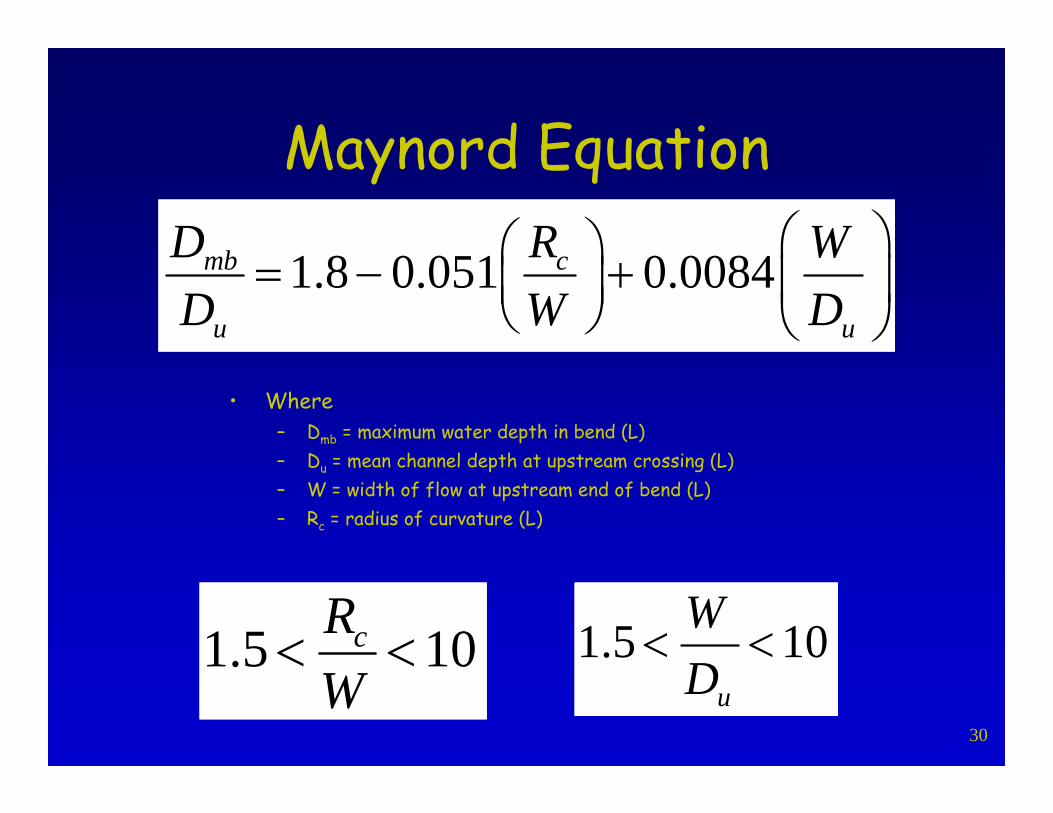
Maynord Equation

• Where– Dmb = maximum water depth in bend (L)– Du = mean channel depth at upstream crossing (L) – W = width of flow at upstream end of bend (L)– Rc = radius of curvature (L)

1.8 0.051 0.0084mb c

u u

D R WD W D

⎞⎛⎞⎛= − + ⎟⎜⎜ ⎟⎝ ⎠ ⎝ ⎠

1.5 10cRW

< < 1.5 10u

WD

< <

31

Maynord Equation

• Notes:– Developed from measured data on 215 sand bed

channels– Flow events between 1 and 5 year return intervals– Not valid for overbank flows that exceed 20 percent of

channel depth– Equation is a “best fit”, not an envelope – NO FOS– Factor of safety of 1.08 is recommended– English or metric units– Width is that of “active flow”

1.8 0.051 0.0084mb c

u u

D R WD W D

⎞⎛⎞⎛= − + ⎟⎜⎜ ⎟⎝ ⎠ ⎝ ⎠

32

Wattanabe Equation

• Where– ds = scour depth below maximum

depth in bend (L)– W = channel top width (L)– Rc = radius of curvature (L)– D = mean channel depth (L)– S = bed slope (L/L)– f = Darcy friction factor

s

c

d WD R

α β⎞⎛

= + ⎟⎜⎝ ⎠

20.361 0.0224 0.0394X Xα = − −

0.2

10log WSXD

⎞⎛= ⎟⎜

⎝ ⎠

1.584 xf

β

π

2=⎧ ⎫⎡ ⎤⎞⎛ 1⎪ ⎪1.226 −⎢ ⎥⎟⎜⎨ ⎬⎜ ⎟⎢ ⎥⎝⎪ ⎪⎠⎣ ⎦⎩ ⎭

1

1.11.5 1.42 sin cos

x

ff

σ σ

=⎡ ⎤⎧ ⎫⎞⎛⎪ ⎪− +⎢ ⎥⎟⎜⎨ ⎬⎜ ⎟⎢ ⎥⎪ ⎪⎝ ⎠⎩ ⎭⎣ ⎦

1 1.1tan 1.5 1.42ff

σ −⎡ ⎤⎧ ⎫⎞⎛⎪ ⎪= −⎢ ⎥⎟⎜⎨ ⎬⎜ ⎟⎢ ⎥⎪ ⎪⎝ ⎠⎩ ⎭⎣ ⎦

33

Wattanabe Equation

• Notes:– Results correlated will with Mississippi River data– Limits of application are unknown– FOS of 1.2 is recommended– English or metric units may be used

s

c

d WD R

α β⎞⎛

= + ⎟⎜⎝ ⎠

34

5 Types of Scour


35

Constriction Scour

36

Constriction Scour

• Occurs when channel features created a narrowing of the channel

• Typically, constriction is “harder” than the channel banks or bed

• Caused from natural and/or engineered features– Large woody debris– Bridge crossings– Bedrock– Flow training structures– Tree roots/established vegetation

37

Constriction Scour

• Scour equations– Developed from flume tests of bridge

abutments– Equations can be applied for natural or

other induced constrictions– Most accepted methods:

• Laursen live-bed equation (1980)• Laursen clear-water equation (1980)

38

Constriction Scour

• Live-bed conditions– Coarse sediments may armor the bed

• Compare with clear-water depth and use lower value

• Requires good judgment!– Equation developed for sand-bed streams– Application to gravel bed:

• Provides conservative estimate of scour depth

39

Laursen Live-Bed Equation

• Where– d = average depth of constriction scour (L)– y0 = average depth of flow in constricted reach without

scour (L)– y1 = average depth of flow in upstream main channel (L)– y2 = average depth of flow in constricted reach after

scour (L)– Q2 = flow in constricted section (L3/T)– Q1 = flow in upstream channel (L3/T)– W1 = bottom width in approach channel (L)– W2 = bottom width in constricted section (L)– A = regression exponent

0.86

2 2 1

1 1 2

2 0

Ay Q Wy Q Wd y y

⎛ ⎞ ⎛ ⎞= ⎜ ⎟ ⎜ ⎟⎝ ⎠ ⎝ ⎠

= −

40

Laursen Live-Bed Equationω = fall velocity of D50 bed material

(L/T)U* = shear velocity (L/T)

= (gy1Se)0.5

g = acceleration due to gravity (L/T2)Se = EGL slope in main channel (L/L)

0.86

2 2 1

1 1 2

2 0

Ay Q Wy Q Wd y y

⎛ ⎞ ⎛ ⎞= ⎜ ⎟ ⎜ ⎟⎝ ⎠ ⎝ ⎠

= −

Suspended0.69>2.0

Suspended0.640.5 to 2.0

Bed0.59< 0.5

Mode of bed Transport

AU*/ω

41


42


• Notes:– Assumes all flow passes through

constricted reach– Coarse sediment may limit live-bed scour– If bed is armored, compare with at clear-

water scour– Both English and metric units can be used

0.86

2 2 1

1 1 2

2 0

Ay Q Wy Q Wd y y

⎛ ⎞ ⎛ ⎞= ⎜ ⎟ ⎜ ⎟⎝ ⎠ ⎝ ⎠

= −

43

Laursen Clear-Water Equation

• Where– d = average depth of constriction scour (L)– y0 = average depth of flow in constricted reach without scour (L)– y2 = average depth of flow in constricted reach after scour (L)– Q2 = flow in constricted section (L3/T)– Dm = 1.25D50 = assumed diameter of smallest non-transportable

particle in bed material in constricted reach (L)– W2 = bottom width in constricted section (L)– C = unit constant; 120 for English, 40 for metric

0.4322

2 0.67 22

2 0

m

QyCD W

d y y

⎛ ⎞= ⎜ ⎟⎝ ⎠

= −

44

Laursen Clear-Water Equation

• Notes:– Only uses flow through constricted section– If constriction has an overbank, separate computation made

for the channel and each overbank– Can be used for gravel bed systems– Armoring analysis or movement by size fraction

0.4322

2 0.67 22

2 0

m

QyCD W

d y y

⎞⎛= ⎟⎜⎝ ⎠

= −

45

5 Types of Scour


17 OCT – address mistake on equation two slides ago

46

Drop/Weir Scour

47

Drop/Weir Scour

• Result of roller formed by cascading flow

• Caused from– Perched culverts– Culverts under pressure flow– Spillway exits– Natural drops in high-gradient mountain

streams

48

Drop/Weir Scour

• Two methods– U.S. Bureau of Reclamation Equation –

Vertical Drop Structure (1995)• Used for scour estimation immediately

downstream of a vertical drop• Provides conservative estimate for sloping

sills– Laursen and Flick (1983)

• Sloping sills of rock or natural material

49

USBR Vertical Drop Equation

• Where– ds = scour depth immediately downstream of drop (m)– q = unit discharge (m3/s/m)– Ht = total drop in head, measured from the upstream to downstream

energy grade line (m)– dm = tailwater depth immediately downstream of scour hole (m)– K = regression constant of 1.9

0.225 0.54s t md KH q d= −

50

USBR Vertical Drop Equation

• Notes:– Calculated scour depth is independent of bed-material grain size– If large material is present, it may take decades for scour to reach final

depth– Must use metric units

0.225 0.54s t md KH q d= −

51

Laursen and Flick Equation

• Where– ds = scour depth immediately downstream of drop (L)– yc = critical flow depth (L)– D50 = median grain size of bed material (L)– R50 = median grain size of sloping sill (L)– dm = tailwater depth immediately downstream of scour hole (L)

0.2 0.1

50

50

4 3cs c m

c

y Rd y dD y

⎧ ⎫⎡ ⎤⎞ ⎞⎛ ⎛⎪ ⎪= − −⎢ ⎥⎨ ⎬⎟ ⎟⎜ ⎜⎢ ⎥⎝ ⎝⎠ ⎠⎪ ⎪⎣ ⎦⎩ ⎭

52

Laursen and Flick Equation

• Notes– Developed specifically for sloping sills constructed of rock– Non-Conservative for other applications– Can use English or metric units

0.2 0.1

50

50

4 3cs c m

c

y Rd y dD y

⎧ ⎫⎡ ⎤⎞ ⎞⎛ ⎛⎪ ⎪= − −⎢ ⎥⎨ ⎬⎟ ⎟⎜ ⎜⎢ ⎥⎝ ⎝⎠ ⎠⎪ ⎪⎣ ⎦⎩ ⎭

53

5 Types of Scour


54

Jet Scour

55

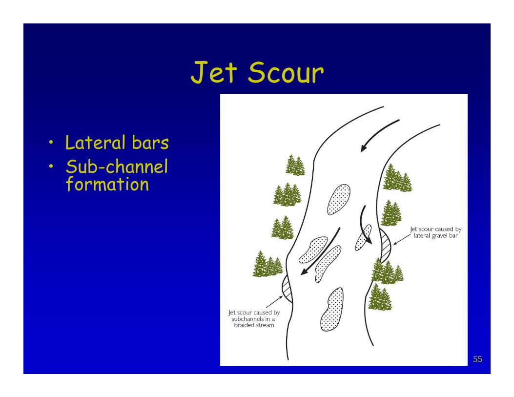
Jet Scour

• Lateral bars • Sub-channel

formation

56

Jet Scour

• High energy side channel or tributary discharges

57

Jet Scour

• Tight radius of curvature

58

Jet Scour

• Very difficult problem to solve• Simons and Senturk (1992) provide

some guidance• Good case for adding a substantial

FOS

59

Jet Scour

60

Jet Scour

61

Jet Scour

62

5 Types of Scour


63

Local Scour

64

Local Scour

• Appears as tight scallops along a bank-line

• Depressions in a channel bed• Generated by flow patterns around an

object or obstruction• Extent varies with obstruction• Can be objective of design

65

Local Scour

• Pier Scour Equations

66

Local Scour

• Pier Scour Equations– Developed for sand-bed rivers– Provides conservative estimate for

gravel-bed systems– Can be applied to other obstructions– Assumes object extends above water

surface– Colorado State University Equation

67

Local Scour

• Colorado State University Equation– Can be applied to both live-bed and

clear-water conditions– Provides correction factor for bed

material > 6 cm – gravel beds– Field verification shows equation to be

conservative

68

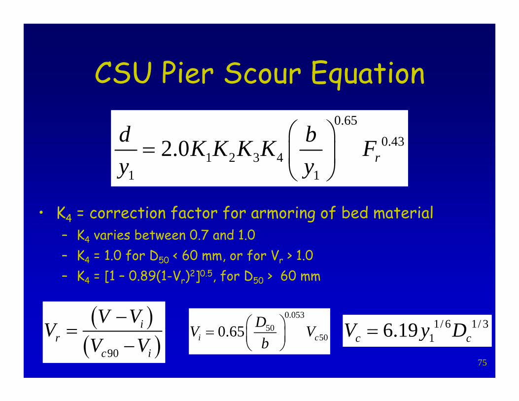
CSU Pier Scour Equation

• Where– d = maximum depth of scour, measured below bed elevation (m)– y1 = flow depth directly upstream of pier (m)– b = pier width (m)– Fr = approach Froude number– K1 – K4 = correction factors

0.650.43

1 2 3 41 1

2.0 rd bK K K K Fy y

⎛ ⎞= ⎜ ⎟

⎝ ⎠

69


• K1 = correction factor for pier nose shape

0.650.43

1 2 3 41 1


⎛ ⎞= ⎜ ⎟

⎝ ⎠

70


• K1 = correction factor for pier nose shape– For angle of attach > 5o, K1 = 1.0– For angle of attach ‹ 5o

• Square nose K1 = 1.1• Circular K1 = 1.0• Group of cylinders K1 = 1.0• Sharp nose K1 = 0.9

0.650.43

1 2 3 41 1


⎛ ⎞= ⎜ ⎟

⎝ ⎠

71


• K2 = correction factor for angle of attach of flow

0.650.43

1 2 3 41 1


⎛ ⎞= ⎜ ⎟

⎝ ⎠

0.65

2LK Cos Sinb

θ θ⎛ ⎞= +⎜ ⎟⎝ ⎠

• Where• L = length of pier (along flow line of angle of attach) (m)• b = pier width (m)• Θ = angle of attach (degrees)

72


• K2 = correction factor for angle of attach of flow

0.650.43

1 2 3 41 1


⎛ ⎞= ⎜ ⎟

⎝ ⎠

5.03.92.5904.33.32.3453.52.82.0302.52.01.5151.01.01.00

L/b = 12L/b = 8L/b = 4Θ

73


• K3 = correction factor for bed conditions– Selected for type and size of dunes– Use 1.1 for gravel-bed rivers

0.650.43

1 2 3 41 1


⎛ ⎞= ⎜ ⎟

⎝ ⎠

74


• K3 = correction factor for bed conditions

0.650.43

1 2 3 41 1


⎛ ⎞= ⎜ ⎟

⎝ ⎠

1.3>9large dunes1.23 to 9medium dunes1.10.6 to 3small dunes1.1n/aplane bed/anti-dune1.1n/aclear water scour

K3Dune Height (m)

Bed Condition

75


• K4 = correction factor for armoring of bed material– K4 varies between 0.7 and 1.0– K4 = 1.0 for D50 < 60 mm, or for Vr > 1.0– K4 = [1 – 0.89(1-Vr)2]0.5, for D50 > 60 mm

0.650.43

1 2 3 41 1


⎛ ⎞= ⎜ ⎟

⎝ ⎠

( )( )90

ir

c i

V VV

V V−

=−

0.05350

500.65i cDV Vb

⎛ ⎞= ⎜ ⎟⎝ ⎠

1/ 6 1/ 316.19c cV y D=

76


• Where– V = approach velocity (m/s)– Vr = velocity ratio– Vi = approach velocity when particles at pier begin to move (m/s)– Vc90 = critical velocity for D90 bed material size (m/s)– Vc50 = critical velocity for D50 bed material size (m/s)– Y1 = flow depth upstream of pier (m)– Dc = particle size selected to compute Vc (m)

0.650.43

1 2 3 41 1


⎛ ⎞= ⎜ ⎟

⎝ ⎠

( )( )90

ir

c i

V VV

V V−

=−

0.05350

500.65i cDV Vb

⎛ ⎞= ⎜ ⎟⎝ ⎠

1/ 6 1/ 316.19c cV y D=

77


• Where– d = maximum depth of scour, measured below bed elevation (m)– y1 = flow depth directly upstream of pier (m)– b = pier width (m)– Fr = approach Froude number– K1 – K4 = correction factors

0.650.43

1 2 3 41 1


⎛ ⎞= ⎜ ⎟

⎝ ⎠

78

Local Scour

• Abutment scour

79

Local Scour

• Abutment scour– Developed for sand-bed systems– Provides conservative estimate for

gravel-bed systems– Can be applied to other obstructions– Results can be reduced based on

experience– Froelich Equation

80

Local Scour

• Froehlich Equation– Predicts scour as a function of shape,

angle with respect to flow, length normal to flow and approach flow conditions

– Provides conservative estimate for gravel-bed systems

– Can be applied to other obstructions– Assumes object extends above water

surface

81

Froehlich Equation for Live-Bed Scour at Abutments

• Where– d = maximum depth of scour, measured below bed elevation (m)– y = flow depth at abutment (m)– Fr = approach Froude number– L’ = length of abutment projected normal to flow (m)– K1 – K2 = correction factors

0.430.61

1 2'2.27 1.0r

d LK K Fy y

⎛ ⎞= +⎜ ⎟

⎝ ⎠

82

Froehlich Equation for Live-Bed Scour at Abutments

• L’ = length of abutment projected normal to flow (m)

θ

0.430.61

1 2'2.27 1.0r

d LK K Fy y

⎛ ⎞= +⎜ ⎟

⎝ ⎠

83

Froehlich Equation

• K1 = correction factor for abutment shape– K1 = 1.0 for vertical abutment– K1 = 0.82 for vertical abutment with wing walls– K1 = 0.55 for spill through abutments

0.430.61

1 2'2.27 1.0r

d LK K Fy y

⎛ ⎞= +⎜ ⎟

⎝ ⎠

84

Froehlich Equation

• K2 = correction factor for angle of embankment to flow

θ

0.430.61

1 2'2.27 1.0r

d LK K Fy y

⎛ ⎞= +⎜ ⎟

⎝ ⎠

85

Froehlich Equation

• K2 = correction factor for angle of embankment to flow

• Where• = angle between channel bank and abutment• is > 90 degrees of embankment points upstream• is < 90 degrees if embankment points downstream

0.13

2 90K θ⎛ ⎞= ⎜ ⎟

⎝ ⎠

0.430.61

1 2'2.27 1.0r

d LK K Fy y

⎛ ⎞= +⎜ ⎟

⎝ ⎠

86

Check MethodU.S. Bureau of Reclamation

87


• Provides method to compute scour at:– Channel bends– Piers– Grade-control structures– Vertical rock banks or walls

• May not be as conservative as previous approaches

88


• Computes scour depth by applying an adjustment to the average of three regime equations– Neil equation (1973)– Modified Lacey Equation (1930)– Blench equation (1969)

89

Neil Equation

• Where– yn = scour depth below design flow level (L)– ybf = average bank-full flow depth (L)– qd = design flow discharge per unit width (L2/T)– qbf = bankfull flow discharge per unit width (L2/T)– m = exponent varying from 0.67 for sand and 0.85 for

coarse gravel

m

dn bf

bf

qy yq

⎛ ⎞= ⎜ ⎟⎜ ⎟

⎝ ⎠

90

Neil Equation

• Obtain field measurements of an incised reach• Compute bank-full discharge and associated hydraulics• Determine scour depth

m

dn bf

bf

qy yq

⎛ ⎞= ⎜ ⎟⎜ ⎟

⎝ ⎠

91

Modified Lacey Equation

• Where– yL = mean depth at design discharge (L)– Q = design discharge (L3/T)– f = Lacey’s silt factor = 1.76 D50

0.5

– D50 = median size of bed material (must be in mm!)

3.3

0.47LQyf

⎛ ⎞= ⎜ ⎟

⎝ ⎠

92

Blench Equation

• Where– yB = depth for zero bed sediment transport (L)– qd = design discharge per unit width (L2/T)– Fbo = Blench’s zero bed factor

0.67

0.33d

Bbo

qyF

=

93

Blench Equation

Fbo = Blench’s zero bed factor

0.67

0.33d

Bbo

qyF

=

94


• Computes scour depth by applying an adjustment to the average of three regime equations– Neil equation (1973)– Modified Lacey Equation (1930)– Blench equation (1969)

• Adjust as follows…

95


• Where– dN, dL, dB = depth of scour from Neil, Lacey and Blench equations,

respectively– KN, KL, KB = adjustment coefficients for each equation

N N N

L L L

B b B

d K yd K yd K y

===

96


KN, KL, KB

0.75 – 1.251.500.4 - 0.7Small dam or grade control

0.50 – 1.00-1.00Nose of Piers

-1.25-Vertical rock bank or wall

-1.00-Right-angle bend

0.600.750.70Severe bend

0.600.50.60Moderate bend

0.600.250.50Straight reach (wandering thalweg)

Bend Scour

Blench-KBLacey-KLNeil-KNCondition

97


• Average values and compare to results of previous methods

• Appropriate level of conservatism??

N N N

L L L

B b B

d K yd K yd K y

===

98

REFERENCES1. Lane, E.W. 1955. Design of stable channels. Transactions

of the American Society of Civil Engineers. 120: 1234-1260

2. U.S. Department of Transportation, Federal Highway Administration. 1988. Design of Roadside Channel with Flexable Linings. Hydraulic Engineering Circular No. 15. Publication No. FHWA-IP-87-7.

3. Richardson, E.V. and S.R. Davis. U.S. Department of Transportation, Federal Highway Administration, 1995. Evaluating Scour at Bridges, Hydraulic Engineering Circular No. 18. Publication No. FHWA-IP-90-017.

4. U.S. Department of Transportation, Federal Highway Administration. 1990. Highways in the River Environment.

5. Thorne, C.R., R.D. Hey and M.D. Newson. 1997. Applied Fluvial Geomorphology for River Engineering and Management. John Wiley and Sons, Inc. New York, N.Y.

99

REFERENCES6. Maynord, S. 1996. Toe Scour Estimation on Stabilized

Bendways. Journal of Hydraulic Engineering, American Society of Civil Engineers, Vol. 122, No.8.

7. U.S. Department of Transportation, Federal Highway Administration. 1955a. Stream Stability at Highway Structures. Hydraulic Engineering Circular No. 20.

8. Laursen, E.M. and Flick, M.W. 1983. Final Report, Predicting Scour at Bridges: Questions Not Fully Answered – Scour at Sill Structures, Report ATTI-83-6, Arizona Department of Transportation.

9. Simons, D.B and Senturk, F. 1992. Sediemnt Transport Technology, Water Resources Publications, Littleton, CO.

10. Bureau of Reclamation, Sediment and River Hydraulics Section. 1884. Computing Degradation and Local Scour, Technical Guideline for Bureau of Reclamation, Denver, CO.

toe and bed scour lectures final 2008 - walter scott, jr ... and bed scour lectures... ·...

Documents