Clay, Conductivity, and Rural Water

Supplies

A hydrogeological investigation

An MSc Dissertation by Gary Clarke

Student ID: B221637

Supervisor: Ian Smout

With the assistance of

Abstract

In regions where the underlying geology is comprised of few aquifers other sources of

groundwater must be tapped into. Mudstones and clay-bearing rocks are traditionally thought

of as being aquicludes. Mudstones and clay-bearing rocks, however, can contain

groundwater in robust fracture networks. The main control as to whether or not these

fractures will develop is the clay type. Smectite clay is poor at developing robust fracture

networks, whereas illite clays can support them. EM34 surveying is a tool used by

geophysicists which determines the conductivity of the subsurface. Borehole, EM34, and clay

analysis data, taken by the British Geological Survey in a region of Nigeria, has been used to

identify a relationship between clay type and measured conductivity. A strong, linear, positive

correlation has been found between measured conductivity and smectite content in the rock.

From this, rural groundwater potential has been inferred by counter-intuitively coming to the

conclusion that areas of low conductivity are likely to hold groundwater in clay-bearing

formations. The findings of the experimental data have been tested against theoretical

models- the Bussian and Revil and Glover equations. The implications of this research within

the WATSAN sector have been explored. Furthermore, information has been presented on

the usefulness of this research in other sectors such as the nuclear industry, engineering

applications, geohazards and remote sensing.

Executive Summary

It is acknowledged that in many water-stressed areas, particularly in Sub-Saharan Africa

(SSA) and Southern Asia, sustainable rural water supplies will be key when it comes to

meeting both present and future demands for clean and plentiful water. WateraAid estimates

that 768 million people globally do not have access to safe water, WaterAid, (2013). This

hydrogeologically orientated project focuses on how to improve successful siting of boreholes

by using geophysics data to infer where groundwater is likely to be plentiful enough to sustain

rural water supplies.

Hydrogeology of Africa and Mudstone Environments

The hydrogeology of SSA can be categorised into four main hydrogeological domains:

crystalline basement rocks, volcanic rocks, consolidated sedimentary rocks, and

unconsolidated sedimentary rocks. Each of these different types of formation has different

porosities and permeabilities, resulting in groundwater being more abundant and accessible in

some formations over others. Mudstones and clay-bearing formations are particularly poor

aquifers. Clays have high porosities (spaces and voids for water to fill) but low permeabilities

(the spaces and voids are not well interconnected). As such they are particularly poor for

sustaining rural groundwater supplies. There are, however, two common ways in which these

sorts of rocks can have acceptable transmissivities. The first of these is the presence of other

subordinate lithologies (rock types) within the main clayey mudstone formation; for example,

having a small sandstone unit within the surrounding clay. Secondly, is the presence of

interconnected fracture networks which allow the groundwater to flow through the clayey

mudstones freely, MacDonald et.al., (2005). It must be stressed that many demographic

regions across the globe lie on top of clayey mudstone formations; therefore it is essential that

any subordinate lithologies or fracture networks can be detected if successful siting of

boreholes is to take place. In regions of water-scarcity these subordinate lithologies and

fracture networks must be tapped into.

The clay type strongly determines whether or not fracture networks will exist. Smectite clays

are soft, plastic weak, and can be easily deformed; consequently any fractures which are

created within smectite clays will easily be squashed away by the pressure of the overlying

rocks. Illite clays, on the other hand, are notably stronger and more resilient to deformation;

therefore robust water-bearing fracture networks can exist in illite clays. Smectite turns into

illite when it is exposed to heat and pressure- this reaction is irreversible. Exposure of rocks

to heat and pressure is more commonly known as metamorphism. The transition of smectite

to illite takes place just before metamorphism during a process of diagenesis.

A common way of resolving sub-surface features is by employing a geophysical surveying

technique called EM34. EM34 is a type of conductivity surveying. Coils generate alternating

magnetic fields which then induce alternating currents within the ground. Comparing the

signal from the source coil and the signal from the receiver coil enables a value of conductivity

of the ground to be determined. It is a type of geophysical surveying commonly used in

developing countries as it is relatively cheap, simple to use, and easy to interpret the data.

The Problem

The problem which this dissertation is trying to solve can be summarised as:

Can geophysical techniques, notably EM34 ground conductivity surveying, be used to

distinguish between different types of clays in the ground?

Many scientists have postulated that such a relationship does exist and many have tried to

quantify it. The first scientist who noted that a rock’s measured conductivity is proportional to

its physical properties was Archie, (1942) - he stated that a rock’s conductivity is linked to its

porosity and the conductivity of the pore water within (in most rocks the main conductors are

the ions within the actual pore water – it is for this reason why high measured conductivity

values imply groundwater abundance). Whilst this relationship has been used extensively by

the hydrocarbon industry with huge success is does not work for clay-rich formations. The

reason for this is because clay minerals/grains have a very high surface conductivity- this

refers to currents which travel along grain surfaces. Surface conductivity is linked strongly to

a property known as ‘Cation Exchange Capacity’ (CEC) which refers to how well positive ions

can move along the surface of a mineral, Wilson, (1994). Because clays have such a strong

CEC (due to them being highly negatively charged) they also have a high surface conductivity.

With clays the effect of the surface conductivity often dwarfs the signal of the pore water

conductivity, therefore both the surface and pore water conductivity must be taken into

consideration.

Data Processing, Analysis and Interpretation

If a relationship between clay type and conductivity exists then it should be possible to

determine different clay types in the ground by using EM34 data. Alan MacDonald of the

British Geological Survey (BGS) has completed extensive EM34 surveying and detailed clay

analysis of fifty boreholes in a water-stressed area in South-Eastern Nigeria. This large and

comprehensive dataset was used to try to identify if a relationship between clay type and

conductivity exists.

Out of the fifty boreholes drilled in the region seventeen of them underwent a process of clay

mineralogy analysis at the BGS’s laboratories in Keyworth, Nottingham. This enables one to

use rock samples taken from different depths down boreholes to determine the amount and

the type of clay present. This dataset was used to calculate the average smectite proportion

in the rocks down-borehole. Each borehole was also sited on an area which had been

surveyed by EM34 equipment. Consequently, every borehole has an associated measured

bulk conductivity value. Knowing both this measured conductivity value and the amount of

smectite present in each borehole it was possible to plot the two against one another. This

dataset was referred to as the ‘gold-star’ dataset as each datum has both a value of measured

conductance and a value of measured smectite proportion. For the other boreholes which

had not undergone clay mineralogy analysis, estimations were made of the likely smectite

proportion in the rocks by using lithological logs of the rock types down the boreholes and

data from the gold-star boreholes. This lead to the creation of an extended dataset which

could be used to determine a relationship between smectite content in the rock and measured

conductivity. The figure below is the graph which represents the relationship.

The data-points are colour coded into the formations which they are part of across the region.

As can be seen, a positive linear relationship does exist. A variance value of 0.89 represents

a good fit to the data. The equation of the line suggests that a rock composed entirely of

smectite would have a conductivity of 352 mS/m and a rock which has no smectite present

whatsoever would have a conductivity of 0.63 mS/m. From the figure above, and by knowing

the transmissivities of each of the boreholes in each of the different formations, the following

new guiding principles have been developed for mudstone/clay-rich formations:

y = 3.5168x + 0.6252 R² = 0.8888

0

20

40

60

80

100

120

140

160

0 5 10 15 20 25 30 35

Co

nd

uct

ivit

y (m

S/m

)

Smectite in rock (%)

Bulk conductivty and inferred smectite proportion in rock for the extended dataset

Gold Star Dataset

Asu River

Lower Eze-Aku

Awgu Shale / Dolerite

Upper Eze Aku

Makurdi

Awgu Shale

Conductivities in the region of 0-40 mS/m are likely to suggest smectite proportions of 0-

11%. It is therefore likely that such areas will be illite rich and have high transmissivities

suitable for rural water supplies.

Conductivities in the region of 40-90 mS/m are likely to suggest smectite proportions of

11-27%. Such areas will have moderate rural groundwater potential.

Conductivities in the region of 90+ mS/m are likely to suggest smectite proportions >27%.

Such areas will have poor rural groundwater potential.

Comparison with Theoretical Models

The next stage was to compare how the findings from this experimental data compared with

what is predicted by theoretical mathematical models. Two mathematical models were tested:

the Bussian, (1983) equation and the Revil and Glover, (1998) equation. Both of these were

extensions of the aforementioned Archie’s Law, but the difference is that these equations take

into account surface conductivities. Investigation proved that the Bussian equation was

mathematically impossible to solve for measured conductivity. The predicted measured

conductivity could be calculated, however, using the Revil and Glover equation. For each of

the boreholes in the gold-star dataset estimations were made as to what the values of certain

parameters would be in the equation. Using the Revil and Glover equation proved to be

unsuccessful. There was no correlation between what was predicted by the model and what

was actually observed with the experimental data. Furthermore, the equation did not even

yield any relationship between smectite content in the rock and the predicted measured

conductivity.

Applications, Significance, and Suggestions

After realising and explaining the reasons why the models were inadequate focus was given

to the significance of the findings of this research. Obviously, the main area where this

research could have the most significant impact is in the WATSAN sector. Two other water

stressed areas have been identified where the findings of this research could be used- the

Karoo Basin, South Africa and the Voltaian Sediments, Ghana. Both areas are predominantly

comprised of clay-rich mudstones, and both have significant abundances of both illite and

smectite. Surveying these areas with EM34 and identifying the regions of low conductivity

could signify illite dominated areas and thus good rural groundwater potential. Both of these

areas are experiencing water scarcity, and with future demand only likely to increase it will be

vitally important to find any water-bearing fracture networks which could be used to sustain

rural water supplies by the means of handpumps. There are other sectors where this

research can be applied. Engineering and geohazards are closely linked. Due to smectite’s

plastic and deformable nature it would not be prudent to lay solid foundations in smectite

dominated areas, as they are likely to deform and slip. Illite dominated areas, on the other

hand, would be safer to build on. Being able to distinguish between smectite and illite

dominated areas using EM34 is a great advantage in this respect. Another hydrogeological

application where the findings could be applied is the siting of a high-level nuclear waste

repository. In a repository groundwater flow must be zero. Most dangerous radioactive

particles are most mobile when in water. Illite’s high potential for groundwater flow means that

illite clays would not be a suitable place to site any repository. Smectite clays, on the other

hand, would be particularly good at keeping out any water. Remote sensing data could also

be used to map illite and smectite areas as satellites can distinguish between high and low

values of cation exchange capacity on the earth’s surface.

The proof that illite clays (which have good groundwater potential) have a low associated

measured conductivity completely changes the way in which boreholes will now be sited in

mudstone/clay-rich environments. Geophysicists and WATSAN professionals need to be

looking for areas of LOW conductivity to signify groundwater potential – which goes

completely against the guiding principle that areas of HIGH conductivity should signify good

groundwater potential. This research will change the way in which new and existing

conductivity data will be analysed in water-stressed mudstone environments hereon in.

References

Archie, G.E., 1942, “The electrical resistivity log as an aid to determining some reservoir

characteristics”, Trans.Am. Inst. Mining Met. Eng., 146, 54-62

Bussian, A.E., 1983, “Electrical conductance in a porous medium”, Geophysics, Vol. 48(9),

pgs. 1258-1268

MacDonald, A.M., Kemp, S.J., Davies, J., 2005, “Transmissivity Variations in Mudstones”,

Ground Water, Vol.43, No.2, pgs 259-269.

Revil, A., Glover, P.W.J., 1998, “Nature of surface electrical conductivity in natural sands,

sandstones, and clays”, Geophysical Research Letters, Volume 25, No.5, pgs. 691-694.

WaterAid, 2013, “Statistics: The hard facts behind the crisis”,

http://www.wateraid.org/uk/what-we-do/the-crisis/statistics, accessed August 2013

Wilson, M.J., 1994, “Clay mineralogy: spectroscopic and chemical determinative methods”,

Chapman and Hall, London, ISBN: 9780412533808

Contents

List of Figures………………………………………………………………………………………....1

List of Tables…………………………………………………………………………………………..2

Glossary and Abbreviations………………………………………………………………………...3

Chapter 1 – Introduction to Clay, Conductivity and Rural Water Supply…………………...5

The Rural Water Supply Problem................................................................................................ 6

Nigeria: A Brief Case Study ......................................................................................................... 7

Groundwater: An Overview ......................................................................................................... 8

African Hydrogeology .................................................................................................................. 8

A Geophysics Approach ............................................................................................................ 10

EM34 ...................................................................................................................................... 11

Electromagnetism and Electromagnetic Induction ............................................................ 11

Conductivity ........................................................................................................................ 12

EM34 Surveying ................................................................................................................. 13

Chapter 2 - Background Study by the BGS……………………………………………………..15

DFID, WaterAid, and the BGS................................................................................................... 15

Geological Triangulation ............................................................................................................ 15

Geological Mapping ................................................................................................................... 16

Geophysical Surveying .............................................................................................................. 18

Siting Boreholes and Estimations of Transmissivities .............................................................. 19

Clay Mineralogy Analysis .......................................................................................................... 19

Factors Controlling the Groundwater Abundance and Distribution Across Oju and Obi .......... 20

Diagenesis and Low-Grade Metamorphism .......................................................................... 20

Other lithologies within the subsurface .................................................................................. 20

Conclusions of the study ........................................................................................................... 21

Chapter 3 - The Problem……………………………………………………………………………22

The Problem in Question ........................................................................................................... 22

Describing the Literature Review Thought Process .................................................................. 23

Searching Strategy ................................................................................................................ 23

Literature Review of Clay and Conductivity ........................................................................... 25

Critical Review of the Literature ............................................................................................. 30

Justifications for investigating the proposed problem ........................................................... 31

Logical Framework................................................................................................................. 32

Chapter 4 - Methodology, Analysis, and Interpretation………………………………………34

Processing Steps ....................................................................................................................... 35

Listing and Cross Referencing the Data ................................................................................ 36

The Hydrogeological Map ...................................................................................................... 36

Correlating Boreholes and EM34 Surveys (Calculation of Bulk Conductivities) ................... 36

Clay Mineralogy Analysis ....................................................................................................... 38

Smectite Content and Bulk Conductivity Relationship .......................................................... 39

Calculation of Clay Mineralogy for other Boreholes .............................................................. 40

Analysis and Interpretations of Findings ................................................................................... 44

Gold-Star Dataset Analysis.................................................................................................... 44

Extended Dataset Analysis .................................................................................................... 44

Interpretations of the findings ................................................................................................ 45

Chapter 5 - Comparison with Theoretical Models……………………………………………..48

Published Theoretical Models (A Short Literature Review) ...................................................... 48

The Bussian Model (1983) ........................................................................................................ 49

The Revil and Glover Model (1998) .......................................................................................... 52

Chapter 6 - Significance and Applications of the Research ………………………………..57

Increased Success at Siting Boreholes and Wells .................................................................... 57

The Karoo Basin Sediments - South Africa, Lesotho, & Swaziland ...................................... 57

The Voltaian Basin Sediments- Northern Ghana .................................................................. 60

Identifying a Suitable Site for a High-Level Nuclear Waste Repository .................................... 62

Engineering Applications ........................................................................................................... 64

Chapter 7 - The Next Steps………………………………………………………………………...66

Suggestions for Further Study ................................................................................................... 66

Applications with Remote Sensing Data ............................................................................... 66

Short Literature Review on Remote Sensing Applications ................................................ 67

Stronger Theoretical and Experimental Agreement .............................................................. 68

A Comprehensive Survey of Water Supply in Oju and Obi Fifteen Years On ...................... 69

Application of the Findings to Other Water Stressed Regions .............................................. 69

Summary of the Findings .......................................................................................................... 70

Closing Remarks ....................................................................................................................... 71

Acknowledgements…………………………………………………………………………………73

References……………………………………………………………………………………………74

Appendices…………………………………………………………………………………………...78

Appendix I…………………………………………………………………………………………….79

Appendix II……………………………………………………………………………………………81

Appendix III…………………………………………………………………………………………...84

Appendix IV…………………………………………………………………………………………..85

1

List of Figures

Figure 1.1 Population with access to drinking water in 1990-2010, Africa, Europe,

………...Southeast Asia, The Americas

Figure 1.2 Percentage of population with access to drinking water in Sub-Saharan Africa

………..in 1990-2010

Figure 1.3 Population with access to drinking water in Sub-Saharan Africa in 1990-2010

Figure 1.4 Rural drinking water trends (Nigeria)

Figure 1.5 The hydrogeological domains of Sub-Saharan Africa

Figure 1.6 Shape and orientation of an electromagnetic wave

Figure 1.7 Bulk conductivity of four layers

Figure 1.8 Vertical coil EM34 set-up schematic

Figure 1.9 Horizontal coil EM34 set-up schematic

Figure 2.1 Geological Triangulation

Figure 2.2 Groundwater Targets in Oju and Obi

Figure 3.1 The microscopic structure of clays

Figure 3.2 Cation Exchange Capacity (CEC)

Figure 3.3 The electric double layer

Figure 3.4 Relationship between clay type and conductivity

Figure 4.1 Locations of boreholes along an EM34 traverse

Figure 4.2 The relationship between smectite content and measured conductivity for the

……….gold-star dataset

Figure 4.3 Lithological log of borehole BGS 5

Figure 4.4 The relationship between smectite content and measured conductivity for the

……….extended dataset

Figure 5.1 Approximation when the Bussian simplified equations are valid

Figure 5.2 Comparison of experimental results and the theoretical model

Figure 5.3 Theoretical and experimental conductivities vs. smectite proportion in rock

Figure 6.1 Schematic representation of the hydrogeology of the Karoo Sediments

Figure 6.2 Geological map of the Karoo Basin

Figure 6.3 Airborne geophysics data of ground conductivity, Northern Ghana

Figure 7.1 LANDSAT data taken over Greater London, UK

2

List of Tables

Table 2.1 A summary of the geological formations across Oju and Obi

Table 3.1 Searching strategy of the literature review

Table 3.2 The logical framework

Table 4.1 Datasets received from the British Geological Survey

Table 4.2 Calculation of smectite proportion in rock

Table 4.3 Clay mineralogy analysis of boreholes in the Awgu Shales formation

Table 4.4 Average values of smectite content for each lithology

Table 4.5 Estimated smectite content for borehole BGS 5

Table 6.1 Water demand, past and future, in the Karoo Basin

3

Glossary and Abbreviations

BGS - British Geological Survey

CEC - Cation Exchange Capacity

DFID - Department for International Development

HLW - High-Level Waste

SSA - Sub-Saharan Africa

VES - Vertical Electrical Sounding

WATSAN - Water and Sanitation

Cation - An ion with a positive charge

Diagenesis - Changes to sedimentary rock caused by variations in temperature and pressure.

The temperature and pressure changes must be significant enough to physically alter the rock

but not so large as to create a new type of metamorphic rock. It often marks the earliest

stages of metamorphism.

Dyke - A vertically orientated igneous intrusion

Ion - A charged particle. An element without a full outer-shell of electrons resulting in a net

positive or negative charge.

Lithological log - A profile with depth, detailing downhole variations in geology (i.e. changes

in rock and soil type). A graphical representation of the sub-surface geology of a particular

site.

Sill - A horizontally orientated igneous intrusion

Sub-strata - The geological rock types and soils beneath the ground surface.

4

A note on the Literature Review

For the purposes of clarity there is no single chapter dedicated to the literature review.

Because of the broadness of the topic at hand it did make sense to have one extremely large

literature review chapter when the information needed to be continuously referred to in other

chapters. The largest literature review section, on clay and conductivity, can be found in

Chapter 3. Smaller reviews of the literature have been presented in Chapter 1 for rural water

supplies, Chapter 5 for mathematical works completed on describing a definitive link between

clays and conductivities, and Chapter 7 for remote sensing applications. Furthermore, a wide

range of literature has been consulted (over fifty references) and is presented throughout the

entirety of the report, and this literature has been scrutinised throughout.

5

Figure 1.1: Distribution of access to different water sources globally from 1990-2010, JMP, (2013a)

Chapter 1- Introduction to Clay, Conductivity, and Rural Water Supply

According to WaterAid’s most recent statistics 768 million people globally do not have access

to safe water, WaterAid, (2013). Whilst this is an extraordinarily high figure of people (more

than 1 in 10 of the world’s population) it must be acknowledged that on the whole progress is

being made. A driver of this is the Millennium Development Goals: targets implemented at the

turn of the millennium, initiated by the UN, to eradicate extreme poverty by 2015. Many

regions across the world have seen a decrease in the percentage of people without access to

improved water supplies. Rapid population growth, however, means that whilst many

percentages may look promising there are infact more people without access to improved

water supplies in many regions. Figure 1.1 is taken from the Joint Monitoring Program for

Water and Sanitation. It shows the distribution of access to different water sources across the

globe. What is easy to appreciate is that the abundance of people without access to improved

6

Figure 1.2: Percentage of people in SSA only with access to surface water and other unimproved supplies, JMP, (2013b)

Figure 1.3: Population of SSA only with access to surface water and other unimproved supplies, JMP, (2013c)

water sources is vastly greater in Africa and South-East Asia than in Europe and the

Americas, as would be expected. Interestingly across Africa more people in 2010 do not have

access to improved water sources compared to 1990 (notice the vast population increase

though).

As would be

expected, there

are vast

differences

between urban

and rural water

supply. Whilst

the previous

statistics referred

to both urban and

rural, this

dissertation is on

rural water supply

with a primary

focus on Sub-

Saharan Africa

(SSA).

Consequently, the

rest of this

document is

focussed on rural

water supplies.

The Rural

Water

Supply

Problem

Rural areas

across SSA face

many different,

albeit no less challenging, water supply problems compared to that of urban water supplies.

7

Figure 1.4: Rural drinking water trends across Nigeria, JMP, (2013d)

Figure 1.2 shows the percentages of people without access to an improved water supply

across SSA. Expressed as a percentage, there have been improvements across the region

for both urban and rural areas in the last twenty years. What is immediately apparent about

Figure 1.2, however, is the stark contrast between the rural and urban areas. In 2010 for

example, 50% of the rural population were using unimproved water sources compared to only

16% of the urban population. The rural water supply problem becomes even more apparent

when you view the same information expressed as a population (Figure 1.3), which shows

that in 2010 274,000 people only had access to an unimproved water supply in the rural areas

compared with only 50,000 in the urban areas (more than five times as many).

Nigeria: A Brief Case Study

With a population nearing 170 million, Nigeria is Africa’s

most populous country. It is widely acknowledged that at

present Nigeria is unable to cope when it comes to

delivering safe water supplies to its rapidly growing

population and around 63.2 million people (approximately

the population of the United Kingdom) do not have

access to safe water; on top of this a further 3 million (66

million in total) have no choice as to what and where their

preferred water supply is, WaterAid Nigeria, (2013).

Figure 1.4 shows rural drinking water trends specifically

for Nigeria. Progress has been made by increasing the

percentage of people of who have access to an improved

water source and there has been a decrease in the

percentage of people using surface water over the

twenty-one year period. The percentage of people using

unimproved water sources has remained constant which

means when taking into consideration Nigeria’s vast

population growth a significantly higher number of people

are using water from an unimproved source. What

Figure 1.4 clearly shows is that Nigeria has a substantial

way to go in improving water sources for its people- a

trend common across many Sub-Saharan African

countries.

This dissertation report uses data collected in a region called Oju and Obi, in Benue State,

South-East Nigeria. Benue State has a population of nearly 5 million inhabitants. Its main

8

industry is food production, signifying that vast quantities of water will be used for irrigation

purposes, Federal Republic of Nigeria, (2013).

Groundwater: An Overview

Ask many people how water moves under the ground and they will think of great underground

caverns and subterranean rivers. Whilst, admittedly, some groundwater does indeed flow in

this way, the majority of it flows through pores in the rock matrix itself, along small joints and

fractures, and occasionally along faults. It is difficult to estimate with any certainty how much

groundwater there actually is. Furthermore, it is even more difficult to say how much of this

groundwater is actually accessible. Price, (1996), delivers a sensible estimation of 54 million

cubic kilometres of groundwater (around 7% of this is actually accessible) exists in the shallow

crust beneath the earth’s surface.

Groundwater is often an excellent source of water to use in rural areas in SSA. During dry

seasons, surface water flows often cease and therefore people need to look for other water

sources. It is usually possible to find some traces of groundwater in the subsurface and

providing the water table is not too deep it should be somewhat accessible. Another

advantage is that groundwater is often plentiful during the dry season. Because it takes time

for rainwater to trickle through the soil and into the rocks beneath, the groundwater peak often

lags behind the rainfall peak (often by many months).

More often than not, aside from groundwater satisfying a quantity need, it also satisfies an

excellent quality need. Groundwater is often of good quality because as the water percolates

through the ground it becomes naturally filtered. Furthermore, due to the time it takes for this

process to happen all pathogens die off. This results in water which poses no microbiological

hazard (unless the groundwater has been extracted from very shallow depths). It is worth

mentioning however, that groundwater can be very high in salt and metal concentrations,

which over prolonged exposure can cause chronic illnesses.

African Hydrogeology

On a local level hydrogeological regimes will be varied and complex. The flow and

abundance of groundwater will be controlled by many factors such as rainfall, recharge,

porosity, permeability, faulting, fracturing, jointing, abstractions, mineral reactions,

lithology/rock type, aquifer catchments, and topography. Fortunately, on a much larger scale

(continent size) the hydrogeology is somewhat simpler to describe.

In the case of the continent of Africa, the hydrogeology and rocks beneath the surface can

essentially be categorised into four main types. MacDonald and Davies, (2000), have

9

Figure 1.5: The hydrogeological domains of Sub-Saharan Africa. The position of Nigeria, the area of focus for this study is noted, MacDonald and Davies, (2000)

described and mapped each of these four major rock types and the following has been

adapted from their work.

10

The four main hydrogeological environments in Africa are as follows; each requires different

means and methods of abstraction as the groundwater will appear at different depths and

within different geological features:

1. Crystalline Basement Rocks- These are the rocks which make up all of the earth’s

continents. They are igneous in their nature and have existed since the early

beginnings of the earth. 220 million rural people in SSA live on them and they occupy

40% of the total land area. Groundwater potential is generally low, but sufficient

quantities can often be found in fracture zones to sustain rural water supply needs.

2. Volcanic Rocks- These rocks occupy 6% of the total landmass and 45 million people

live on them. They lie, unsurprisingly, around the volcanous regions of SSA and are

especially common on the drought stricken areas of the Horn of Africa- a region where

the continent is literally trying to tear itself apart. Volcanic rocks are often extremely

porous and permeable in nature because when they are solidifying gas bubbles out of

them and leaves open many pathways and channels. Because of this, groundwater

potential is high.

3. Consolidated Sedimentary Rocks- Occupies 32% of the land area and 110 million

people live on them. They consist of sandstones and limestones (good groundwater

supply potential) and mudstones (poor groundwater supply potential. They account

for two thirds of all sedimentary rocks in SSA).

4. Unconsolidated Sediments- Occupies 22% of the land area and sustains a rural

population of 60 million. These comprise of silt, sand and gravels often found in river

beds and on deltas. During wet seasons they can yield good quantities of

groundwater, however, because the groundwater is usually very shallow it can deplete

during the dry season and can be of poor quality.

Figure 1.5 summarises the distribution of each of these rock formations described above on a

map of SSA. Observation of Nigeria specifically shows that the main types of hydrogeological

domain in the country are the Pre-Cambrian crystalline basement rocks and consolidated

sedimentary rocks. The area under study for this research project, Oju and Obi, lies on

consolidated sedimentary rock, most of which is made up of mudstone - the type of rock which

has the poorest groundwater potential across the whole of Africa. Therefore, in order to try to

improve the ability to access such small, but desperately needed, quantities of groundwater in

such regions is a worthwhile endeavour.

A Geophysics Approach

Geophysics is a powerful tool which can be used to identify or infer the presence of

groundwater in the subsurface. It essentially is a way of using various equipment to make

measurements of the physical properties of the subsurface. Through not understanding how

11

Figure 1.6: A schematic diagram representing the shape and orientation of an electromagnetic wave

priceless geophysics data can be or by not knowing how to carry out surveying correctly, time

and time again professionals in the WATSAN sector waste vast amounts of time, money and

energy drilling holes in the ground which never have any chance of sustaining rural water

supply.

EM34

EM34 is a type of non invasive surveying technique and is the type of surveying used in this

dissertation report. It falls under the wider umbrella term of Electromagnetic Surveying: so

named because it uses the phenomena of electromagnetic induction to “see” beneath the

earth’s surface.

Electromagnetism and Electromagnetic Induction

Electromagnetism was first

described mathematically and

comprehensively by the

Scottish physicist James Clerk

Maxwell. Electromagnetism is

the study of electromagnetic

waves and fields. These

waves (of varying wavelength

and frequency) are

composed of both electric

fields and magnetic fields

which are orientated perpendicular to one another (Figure 1.6). Although Maxwell was the

first scientist to be accredited with a full mathematical description of these waves, their

existence had been known about for quite some time.

Michael Faraday famously noted the phenomena of electromagnetic induction (on which

EM34 surveying is based). By placing two coils of wire close together, but not touching, he

noticed that by passing a changed electrical current through the first wire an electrical current

also flowed through the second wire. Although not fully understood at the time, Faraday had

discovered the process of electromagnetic induction.

Electrical currents have electrical fields associated with them. Any charged particle (such as

electrons or ions) has an electric field associated with it. This field technically extends for an

infinite distance, but the force which another charged particle will experience when in the

electrical field will quarter every time you double the distance separating the particles, so that

electrical fields become negligible after relatively small distances. When you have a varying

current (and thus a varying electric field) within a wire you create a varying magnetic field.

This varying magnetic field extends throughout free space and then creates a voltage (and

12

Figure 1.7: Schematic bulk conductivity of four layers within the earth. The ovals are the coils and the blue line represents the signal path.

Figure 1.8: Vertical coil EM34 set-up. The bottom cross section represents the surveying taking place whilst the top graph corresponds to the signal response over each feature. Note the peak over the dolerite.

thus an electrical current) in

a wire some distance away.

This is the process of

electromagnetic induction

and is how EM34 works.

Conductivity

Conductivity refers to how

well a particular material

can facilitate the movement

of charge (also known as

current). Its inverse is

referred to as resistivity, i.e.

if a material has high

conductivity it will have a

low resistivity and vice

versa. Materials which are

good at conducting are

known as conductors and

those which are not are

referred to as insulators.

Even insulators will be able

to conduct some electricity,

albeit very weakly. There

are many different

mechanisms by which

current can move throughout

a material. In rocks, the two

most common ways are

through the bulk of the

material (usually very weak)

and through the pore water

which exists in-between the

individual particles (usually

very strong).

In this report there will be

three terms used throughout:

conductivity, bulk

13

Figure 1.8: Horizontal coil EM34 set-up. The bottom cross section represents the surveying taking place whilst the top graph corresponds to the signal response over each feature. Red lines are faults, blue lines are fractures. The yellow dots and brown dashes represent different geological units.

conductivity, and measured

conductivity. Technically these

three terms have different

meanings, but in this report the

terms have been used

interchangeably (as this is

geological convention).

Nevertheless, an appreciation

should be given to what each

of these terms actually mean.

Conductivity (often referred to

as actual or true conductivity) is

the specific value of

conductivity for one particular

medium. Measured

conductivity relates to what the

instrumentation actually

measures. Figure 1.7

illustrates the concept of bulk

conductivity. Each of the four

layers has its own conductivity

(σ1, σ2, σ3, σ4). The

instrument, however, does not

display a value for each of

these four layers. What it

actually displays is a value of bulk conductivity which is a contribution of each of the

conductivities from each layer. Throughout this report, unless specified otherwise, when one

of these three terms is used it actually is referring to the bulk conductivity.

EM34 Surveying

EM34 surveying is a common form of surveying technique used in developing countries. The

reason for this is because it is relatively cheap, easy to operate, and easy to interpret the data.

Two coils are used, one is a transmitter and the other is a receiver. The transmitter emits a

varying magnetic field, which then induces a varying electrical current beneath the ground.

This varying electrical current then creates a varying magnetic field which is detected by the

receiver coil. Figures 1.8 and 1.9 show how EM34 works by having a cross section of the

geology and the signal response for both the vertical and horizontal coils. As can be seen,

different coil orientations are sensitive to different features beneath the ground.

14

This report will now go on to explain the details, findings and interpretations, and discussion of

the project in detail.

15

Figure 2.1: Geological Triangulation

Chapter 2- Background Study by the BGS

This chapter provides a background for the reader concerning the work conducted by the

British Geology Survey (BGS) in Oju and Obi, Benue State, Nigeria, upon which this

dissertation is based. The information contained within this chapter is based upon the work of

Dr Alan MacDonald and his team, and most of the information presented is sourced from his

reports and also from person discussion.

DFID, WaterAid, and the BGS

The region of Oju commonly experiences severe drought issues in the dry season. During

this season water is scarce, and the primary source of drinking and domestic water used to be

unprotected ponds and seepages. Water related diseases, such as guinea worm, malaria,

cholera, typhoid and dysentery were prevalent amongst the 300,000 strong population. DFID

commissioned WaterAid to improve village level, domestic water supply by primarily exploiting

groundwater. WaterAid drilled a borehole in the centre of the region but ironically it did not

yield any significant amounts of water. The region has a complex hydrogeological profile and

consequently WaterAid asked the BGS to provide assistance, and work began in September

1996, MacDonald and Davies, (1997); this same report discusses in detail the climate, river-

flow, rainfall, and basic geology

of the Oju area.

Geological

Triangulation

To estimate the hydrogeological

potential of the area the BGS

employed a technique known as

‘geological triangulation’.

Geological triangulation

essentially enables you to

estimate the groundwater

potential of a site by extracting

information from three different

sources prior to drilling. Figure

2.1 illustrates this technique and is

16

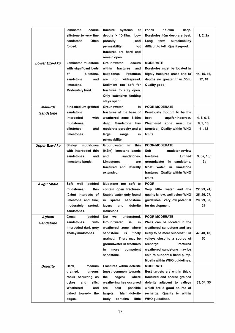
Table 2.1: A summary of the geological formations across Oju and Obi

taken from MacDonald and Davies, (no date). Each of these three main sectors has their own

merits but all should be treated with equal importance! Maps enable you to identify where the

best places would be to conduct your geophysics. Hydrogeological maps will allow you to

identify where potential major aquifers could lie and they narrow down the region where you

would aim to conduct costly and time consuming geophysics. Geophysics is the only method

which truly enables you to ‘see’ beneath the ground surface and try to spot groundwater within

the underlying rocks. Observations, however, can be an invaluable tool. Local knowledge

from communities in particular is often priceless and they can tell you where there is good

river flow, the location of springs etc, which can all lead to increased success of finding rural

groundwater supplies. Using these three sources in unison gives you your best shot at being

able to find and exploit sustainable rural water supplies.

Observations and consultations with each community can be found in a series of village

reports by the BGS (unpublished); they also contain information regarding what boreholes the

BGS drilled in and around each village and the water quantity and quality which they

delivered. The reader should contact Alan MacDonald of the BGS personally if they wish to

read in more detail the findings of each of these reports, as they are not freely available in the

public domain.

Geological Mapping

MacDonald and his team ensured that comprehensive geological mapping of Oju and Obi

took place before conducting any geophysical surveying; they also mapped the precise

locations of the villages with GPS coordinates - something which had not been done before

(see MacDonald and Davies, (1998)). The maps which they produced are found in

APPENDIX I. The various formations which make up Oju and Obi are presented in Table 2.1;

this also includes the borehole numbers BGS(No.) which were drilled in the formation. The

information in Table 2.1 is sourced from Davies and MacDonald, (1999).

Formation Geology Hydrogeology Groundwater Potential Boreholes BGS ( )

Metamorphosed Asu River

Hard, splintery, slatey, mudstones. Sandstones, limestones, ash layers, dolerite, and gabbro are minor lithologies. Highly fractured.

Good aquifer. Rocks have low porosity and permeability but high degree of fracturing. Fractures are hard and remain open. Ash layers- best targets, fractured bedrock good.

HIGH Significant groundwater within fractures below 11m and in ash layers. Less groundwater where bedrock was less metamorphosed. Quality-good-within WHO guidelines.

19, 20, 21

Asu River Hard splintery mudstones and

Groundwater occurs within widespread

HIGH Best targets are fracture

17

laminated coarse siltstone to very fine sandstone. Often folded.

fracture systems at depths > 10-15m. Low porosity and permeability but fractures are hard and remain open.

zones 15-50m deep. Boreholes 40m deep are best. Long term sustainability difficult to tell. Quality-good.

1, 2, 2a

Lower Eze-Aku Laminated mudstone with significant beds of siltstone, sandstone and limestone. Moderately hard.

Groundwater occurs within fractures and fault-zones. Fractures are not widespread. Sediment too soft for fractures to stay open. Only extensive faulting stays open.

MODERATE Boreholes must be located in highly fractured areas and to depths no greater than 30m. Quality-good.

14, 15, 16, 17, 18

Makurdi Sandstone

Fine-medium grained sandstone interbeded with mudstones, siltstones and limestones.

Groundwater in fractures at the base of weathered zone 8-15m deep. Sandstone has moderate porosity and a large range in permeability.

POOR-MODERATE Previously thought to be the best aquifer-incorrect. Weathered zone must be targeted. Quality within WHO limits.

4, 5, 6, 7, 8, 9, 10, 11, 12

Upper Eze-Aku Shaley mudstones with interbeded thin sandstones and limestone bands.

Groundwater in thin (0.3m) limestone bands and sandstones. Limestones are fractured and laterally extensive.

POOR-MODERATE Soft mudstones=few fractures. Limited groundwater in sandstone. Most water in limestone fractures. Quality within WHO limits.

3, 3a, 13, 13a

Awgu Shale Soft well bedded mudstones, thin (0.5m) interbeds of limestone and fine, moderately sorted, sandstones.

Mudstone too soft to contain open fractures. Usable water only found in sparse sandstone layers and dolerite intrusions.

POOR Very little water and the quality is low, well below WHO guidelines. Very low potential for development.

22, 23, 24, 25, 26, 27, 28, 29, 30,

31

Agbani Sandstone

Cross bedded sandstones with interbeded dark grey shaley mudstones.

Not well understood. Groundwater is in weathered zone where sandstone is finely grained. There may be groundwater in fractures in more competent sandstone.

POOR-MODERATE Wells can be located in the weathered sandstone and are likely to be more successful in valleys close to a source of recharge. Fractured weathered sandstone may be able to support a hand-pump. Mostly within WHO guidelines.

47, 48, 49, 50

Dolerite Hard, medium grained, igneous rocks occurring as dykes and sills. Weathered and baked towards the edges.

Fractures within dolerite (most common towards the edges) where weathering has occurred are best possible targets. Main dolerite body contains little

MODERATE Best targets are within thick, fractured and coarse grained dolerite adjacent to valleys which are a good source of recharge. Quality is within WHO guidelines.

33, 34, 35

18

groundwater.

Laterite This is weathered material referred to as a regolith. Soils and clay rich zones.

Highly permeable rock and shallow groundwater does exist in top soils.

SEASONAL Water present in wet season but not in the dry. Vulnerable to contamination from pit latrines. Quality is below WHO guidelines.

None drilled

Alluvium Very little present, river gravels.

Sufficient water for a hand dug well. Permeable material.

POOR Little groundwater storage available.

Cannot be drilled due

to fine sediment

infiltration.

The reader is encouraged to refer to this table and the maps in the appendices whilst reading

interpretation sections in the rest of the report.

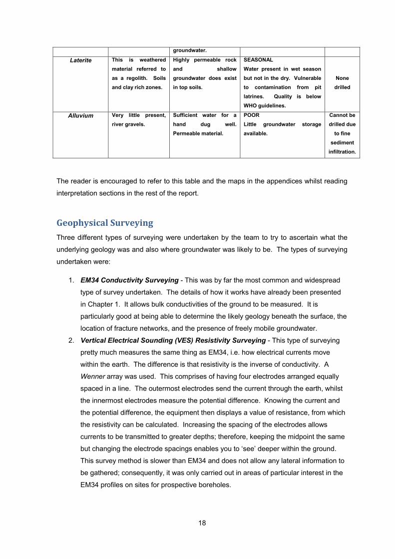
Geophysical Surveying

Three different types of surveying were undertaken by the team to try to ascertain what the

underlying geology was and also where groundwater was likely to be. The types of surveying

undertaken were:

1. EM34 Conductivity Surveying - This was by far the most common and widespread

type of survey undertaken. The details of how it works have already been presented

in Chapter 1. It allows bulk conductivities of the ground to be measured. It is

particularly good at being able to determine the likely geology beneath the surface, the

location of fracture networks, and the presence of freely mobile groundwater.

2. Vertical Electrical Sounding (VES) Resistivity Surveying - This type of surveying

pretty much measures the same thing as EM34, i.e. how electrical currents move

within the earth. The difference is that resistivity is the inverse of conductivity. A

Wenner array was used. This comprises of having four electrodes arranged equally

spaced in a line. The outermost electrodes send the current through the earth, whilst

the innermost electrodes measure the potential difference. Knowing the current and

the potential difference, the equipment then displays a value of resistance, from which

the resistivity can be calculated. Increasing the spacing of the electrodes allows

currents to be transmitted to greater depths; therefore, keeping the midpoint the same

but changing the electrode spacings enables you to ‘see’ deeper within the ground.

This survey method is slower than EM34 and does not allow any lateral information to

be gathered; consequently, it was only carried out in areas of particular interest in the

EM34 profiles on sites for prospective boreholes.

19

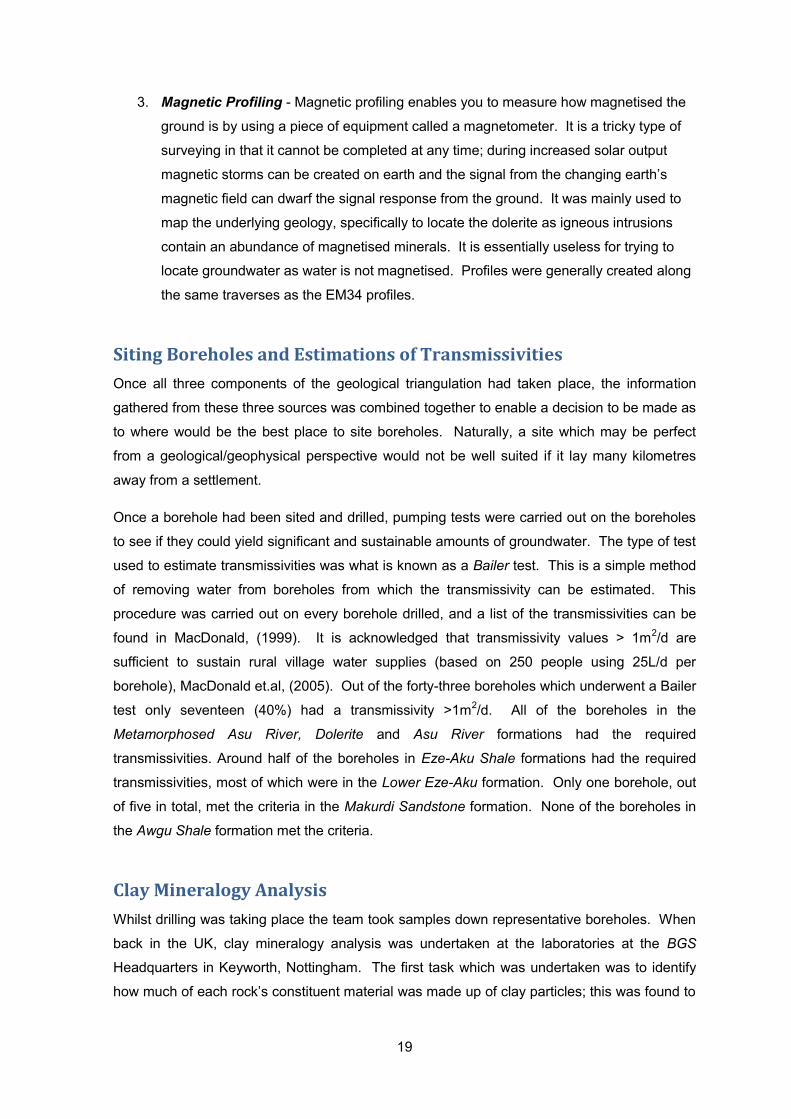
3. Magnetic Profiling - Magnetic profiling enables you to measure how magnetised the

ground is by using a piece of equipment called a magnetometer. It is a tricky type of

surveying in that it cannot be completed at any time; during increased solar output

magnetic storms can be created on earth and the signal from the changing earth’s

magnetic field can dwarf the signal response from the ground. It was mainly used to

map the underlying geology, specifically to locate the dolerite as igneous intrusions

contain an abundance of magnetised minerals. It is essentially useless for trying to

locate groundwater as water is not magnetised. Profiles were generally created along

the same traverses as the EM34 profiles.

Siting Boreholes and Estimations of Transmissivities

Once all three components of the geological triangulation had taken place, the information

gathered from these three sources was combined together to enable a decision to be made as

to where would be the best place to site boreholes. Naturally, a site which may be perfect

from a geological/geophysical perspective would not be well suited if it lay many kilometres

away from a settlement.

Once a borehole had been sited and drilled, pumping tests were carried out on the boreholes

to see if they could yield significant and sustainable amounts of groundwater. The type of test

used to estimate transmissivities was what is known as a Bailer test. This is a simple method

of removing water from boreholes from which the transmissivity can be estimated. This

procedure was carried out on every borehole drilled, and a list of the transmissivities can be

found in MacDonald, (1999). It is acknowledged that transmissivity values > 1m2/d are

sufficient to sustain rural village water supplies (based on 250 people using 25L/d per

borehole), MacDonald et.al, (2005). Out of the forty-three boreholes which underwent a Bailer

test only seventeen (40%) had a transmissivity >1m2/d. All of the boreholes in the

Metamorphosed Asu River, Dolerite and Asu River formations had the required

transmissivities. Around half of the boreholes in Eze-Aku Shale formations had the required

transmissivities, most of which were in the Lower Eze-Aku formation. Only one borehole, out

of five in total, met the criteria in the Makurdi Sandstone formation. None of the boreholes in

the Awgu Shale formation met the criteria.

Clay Mineralogy Analysis

Whilst drilling was taking place the team took samples down representative boreholes. When

back in the UK, clay mineralogy analysis was undertaken at the laboratories at the BGS

Headquarters in Keyworth, Nottingham. The first task which was undertaken was to identify

how much of each rock’s constituent material was made up of clay particles; this was found to

20

be approximately fifty percent in most cases. Furthermore, it allowed the team to identify what

type of clay minerals were present and in what proportions: kaolinite, illite, and smectite most

notably. Further details on the clay mineralogy data including relative proportions are present

in greater deal in Chapter 4. Full tables are available in Appendix 2 of Macdonald, (1999).

Factors Controlling the Groundwater Abundance and Distribution

Across Oju and Obi

It is hypothesised by MacDonald et.al., (2005), that transmissivity in the mudstone dominated

region is primarily controlled by two main factors. The first one is low-grade metamorphism

and the second is the presence of other smaller lithologies within the subsurface. These two

factors are now discussed and the information presented is sourced from the same paper.

Diagenesis and Low-Grade Metamorphism

Diagenesis is an early form of metamorphism. It refers to physical changes which occur to

sedimentary rocks due to changes in heat and pressure, but changes which are not so great

as to create a new metamorphic rock. It is the early stage, and onset, of prograde

metamorphism. The conversion of smectite → illite/smectite → illite→ muscovite is an

example of an irreversible transformation from diagenesis to low-grade metamorphism,

Merriman and Peacor, (1999).

The youngest formation across Oju and Obi is the Awgu Shale Formation. It has not

undergone any significant burial (hence small/no increase in pressure and temperature) and

has, therefore, an abundance of smectite dominated clays. The oldest formation, however,

the Asu River Group, has undergone sufficient burial and folding and therefore is dominated

by illite clays. Across Oju and Obi, travelling from NW to SE, there is a decreasing abundance

of smectite matched by an increasing abundance of illite. Travelling in the same direction,

there is also an increased groundwater potential suitable for sustainable rural water supplies.

Therefore it is clear that as metamorphism, and thus illite, increases so does transmissivity.

Other lithologies within the subsurface

The other main suitable groundwater targets in the Oju/Obi area were the dykes and sills

which were located primarily in the Awgu Shales formation. Dykes and sills are igneous

intrusions. Igneous intrusions are rocks which have been thrust upwards through the crust

towards the surface. Usually they are poor groundwater targets and they often act as barriers

to groundwater flow, Bromley et.al, (1994). A good groundwater target in relation to the dykes

and sills is the contact zone between the igneous intrusions and the surrounding rocks.

Figure 2.2 is a schematic diagram representing the various groundwater targets in the Oju/Obi

area, taken from MacDonald et.al, (2005).

21

Figure 2.2: Groundwater targets in Oju and Obi

Conclusions of the study

The project successfully identified the best areas in Oju/Obi where groundwater can be used

as a sustainable rural water source. The general trend noticed was that the groundwater

potential and transmissivities increase as you move from NW to SE with increasing illite

content. Whilst it is acknowledged that subordinate lithologies within the mudstones can yield

some groundwater supplies, groundwater potential is mainly controlled by the relative

abundances of smectite and illite in the rocks - this determines whether or not suitable fracture

networks can develop.

Once the boreholes were drilled, the ones with sufficient transmissivities were developed to

provide the citizens of Oju and Obi with clean and sustainable domestic/drinking water. Whilst

this relationship between smectite and illite abundance was noted by the team, it has not been

pursued and investigated any further. It has been realised that being able to distinguish

between smectite and illite in the subsurface by using non-invasive geophysical techniques

would be a huge advantage in the hunt for locating rural groundwater supplies. Consequently,

the data collected from this BGS project has been used in this dissertation to see if such a link

can be made. Chapter 3 goes on to discuss in more detail the problem which this dissertation

is addressing.

22

Chapter 3 - The Problem

Anything which furthers our understanding on groundwater and how to detect it will lead to

increased success rates of drilling boreholes and wells and striking groundwater of sufficient

quality and quantity to lead to sustainable rural water supplies. As such, furthering our

understanding is a worthwhile endeavour, and consequently the author has chosen to

dedicate his time for this research project to do just that.

The Problem in Question

This particular problem was brought to the author’s attention by Dr Alan MacDonald, Principle

Hydrogeologist of the BGS Edinburgh. Their work, which his team and he carried out, has

already been discussed in the previous chapter to give the reader a flavour of the background

and motivation of this project. In essence, the problem can be summarised in the following

question:

Can geophysical techniques, notably EM34 ground conductivity surveying, be used to

distinguish between different types of clay in the ground?

Upon first glance, the reader may question what this problem has to do with water supply. Put

simply, in areas where there are extremely small amounts of groundwater to look for the

groundwater directly using geophysical surveying techniques is difficult. Therefore, one must

look at being able to identify clues in the underlying geology which suggests that groundwater

may be present. Essentially, the clay type can indicate whether or not water will be present;

therefore being able to distinguish between different clay types is a powerful tool when it

comes to siting boreholes and wells.

Whilst there are many hundreds of different types of clay minerals present on earth there are

four main ones which are common and are the focus of this study: kaolinite, smectite,

smectite/illite (a transition phase), and illite. Smectite is soft, plastic, weak, and can be easily

deformed. Illite, on the other hand, is notably stronger and more resilient to deformation.

Smectite is essentially converted to illite through processes of diagenesis and early

metamorphism. Fractures in smectite will soon be squashed away from the pressure of the

overloading rocks/sediment. Fractures in illite, however, will not easily be squashed; they will

maintain their shape and allow water to flow through with ease. In areas of unfavourable

aquifer geology, i.e. areas which are dominated by a significant proportion of clay, being able

to target these robust fractures in illite dominated rocks is key to being able to deliver

sustainable rural water supplies.

23

It should be noted that clay is usually what is referred to as an aquiclude - a rock which does

not yield significantly high amounts of water. Clay is very porous, meaning it has a lot of holes

and gaps, both within and in-between mineral grains, which can hold water. The problem,

however, is that it is not very permeable, meaning that these voids and pore spaces are not

well interconnected meaning that water cannot flow. Knowing this fact, many areas around

the world have been simply written-off as areas which cannot sustain rural groundwater

supplies. In the most water-stressed regions of the world, such as SSA, water sources can be

so few and far between that even the smallest supplies of groundwater must be tapped into.

Therefore, being able to tap into fracture networks present in illite-clay rocks is essential to

sustain people’s livelihoods and general well-being.

Describing the Literature Review Thought Process

Once the problem had been identified the next step was to complete a literature review.

Conducting a literature review allows the following points to be address:

Is the problem a new topic which needs to be investigated? Has anyone already

answered the problem?

What information has already been written on the subject?

With the information already out there, how reliable is this information? Does it need

to be scrutinised? Does it make sense?

The literature review will build up one’s own knowledge and capacity to answer the

problem.

It enables the problem to be tweaked and tailored to answer something specific which

has not been addressed in so much detail before.

Searching Strategy

To search for relevant information certain keywords had to be used in order to access this

relevant information. Examples of relevant keywords and phrases are given.

KEYWORDS: EM34, resistivity, geophysics, geophysical, surveying, surveys, electrical conductivity, electrical conductivity of rocks/clays/minerals, clay(s), smectite, illite, CEC (cation exchange capacity), surface conductivity, pore water (electrolyte) conductivity, double-layer, surface conductivity models, macroscopic, microscopic, Oju and Obi, African (hydro)geology.

The above keywords and phrases have been grouped (using different colours) in order to

distinguish topics which are similar and synonyms. Combinations of the above words were

used to source suitable information.

24

Table 3.1: Searching strategy of the literature review

Table 3.1 describes the various sources of information used to complete the literature review,

the searching strategy, the justification of approach, and the quality controls.

Source of Information

Search Strategy Justification of Approach

Evaluation to ensure quality

Library Catalogue Primarily using the advanced search and selected key databases. Inserting the keywords listed above in sensible combination.

Enables a wide range of databases to be searched and accessed. Different types of media can be found (i.e. journals, books, magazines etc…). High volume of results.

Peer reviewed journals accessed, and books have been published which have been reviewed, checked, and updated.

Library Browsing The geology section on the ground floor of the Pilkington library enables browsing of book titles on the subject topic, enables discovery of key materials.

As the problem is quite specific the majority of the information needed can be sourced from the same section of the library. Enables you to pick up key materials which may have been missed when searching the library databases.

Peer reviewed journals accessed, and books have been published which have been reviewed, checked, and updated.

WEDC Resources

Centre Browsing

Enables browsing of a range of materials specifically related to the WATSAN sector.

Context specific information available. Information often sorted into country-specific folders allowing relevant information to be found.

WEDC is a world leading institution with a reputable scientific appreciation. Resource centre manager has a phenomenal understanding of the literature and information in the centre.

Journals Primarily accessed through Library Catalogue. Once key titles had been identified, i.e. “Journal of Applied Geophysics”, searching using the keywords above could be conducted on these journals websites.

Journals are going to be the primary material type to source information from. Often available in electronic format. Allows a snowballing effect- from one journal you may get three other references which you want to then go and find more information on.

Journals are peer reviewed, meaning that their quality is checked and authenticated by other leading academics in the field. Try to use journals as recent as possible to ensure information isn’t outdated.

Textbooks Mainly found from the Library Catalogue, also by library browsing. Reading the chapter list and index allows you to find the relevant information more

Textbooks contain a wide range of information on a very specific subject. Tend to give you a more general overview of the subject than journals

All books used were either from the Pilkington Library, WEDC resources centre, or books which I own based on recommendations from

25

quickly. Skimming certain chapters again can help you find more relevant information.

which tend to be very case-study-specific.

academics in this field.

PhD Thesis Thesis used was Dr Alan MacDonald’s own research project personally sent to me by him. Searching not really required.

Subject specific case studies of the topic, knew that they contained relevant information.

Information within was deemed to be of a high enough standard for a PhD to be awarded. Same information repeated in many published articles.

Personal Experience Searching not required. Know that previous investigations are relevant to this problem statement.

Built up knowledge over many years on this subject.

Private Discussions Discussion with supervisor Ian Smout and Alan MacDonald.

Allows a vast amount of information to be gathered and allows you to bounce ideas and thoughts off of others.

Both are experts in their respective fields and have personal experience of some of the problems discussed.

Articles New Scientist, Science, and other articles were read. Individual articles were searched through the magazines’ websites.

References within these articles were followed up and these have been referenced.

Quality is difficult to check, hence only used in this report if there were credible references attached to the articles which were further investigated to verify claims.

Government Websites Websites BGS, and NERC Open Access were searched to find relevant information.

Governments conduct and pay for a vast amount of geological research. The data collected is often very useful and available in the public domain.

Government supported departments ran by leading academics in the field of geology/geophysics.

Google/(Scholar) Keywords typed-in in a coherent and sensible order/combination, brings up some key journal articles.

Easy to use, good first step in scoping what information is already out there.

Information only included in report if it came from a reputable source, i.e. peer reviewed journal, government website etc…

Literature Review of Clay and Conductivity

The first piece of information that has to be sourced, is how do rocks (and more importantly

clays) actually conduct electrical currents? Appreciation of how rocks/clays conduct will

enable us to determine whether or not they can be identified using electromagnetic surveying

techniques. Kearey et.al, (2002), states that the conductivity of a particular specimen is

dependent upon the chemical composition, size, shape and orientation of the grains. It is also

strongly influenced by porosity and the abundance of fractures due to the main conductors in

26

Figure 3.1: The microscopic structure of clays. Usually micro-metres in size.

rocks being freely mobile ions. As early on as the 1940’s, Archie, (1942), noted how the

electrical conductivity of rocks can be related to its physical properties. The formula he

created (see below) has been used as a firm foundation for all other subsequent relationships

derived to match electrical conductivity to physical properties. It has been used with great

success frequently by the hydrocarbon industry.

Archie’s Law

Where…

σ0 = measured conductivity of the rock

σw = conductivity of the pore water

φ = porosity

m= constant

F= formation factor

The problem with this rather simple

formula is that it is only really dependent

on the porosity and the ion abundance

within the rock. In clays it is well known

that the majority of currents pass along the

actual grain surfaces, which Archie’s Law

does not take into consideration.

To understand what makes conductivity in

clays unique we need to first understand

the microscopic structure and properties of

clays in general (and more specifically for

this study, smectite and illite). Clays are

often thought of as being plate-like in

shape. Clay particles have incredibly large

surface areas relative to their volume.

Bergaya and Langaly, (2006), describe

simply how clays are made up; Figure

3.1 has been adapted from their work. These assemblies of clay minerals are held together

by electrostatic forces. Clay layers are highly charged and as a consequence, layers are

attracted together to make particles, particles are attracted together to make aggregates etc…

27

Figure 3.2: Cation Exchange Capacity (CEC). Notice the swapping movement of the blue and pink positive ions on the clay surface.

It is because of these

highly charged

surface areas that a

substantial amount of

current travels along

the surfaces in clayey

materials, and the

reason why simple

formulas, such as

Archie’s Law, cannot

be used.

What needs to be

taken into consideration is a phenomenon known as Cation Exchange Capacity (CEC) -

something particularly prevalent in clays. Wilson, (1994), defines CEC as:

The sum of exchangeable cations that a mineral can absorb, at a specific pH, i.e. a

measurement of the negative charges carried by the mineral.

Put simply, this refers to how well positive ions (cations) can move along the surface of a clay

mineral. Clay surfaces are highly negatively charged; consequently they attract positively

charged ions to their surface. When a voltage is applied to the clay minerals, the cations

which were stuck to the clay surface can be replaced by other cations which are in solution

nearby. This swapping movement of charge creates a current which can be detected. Figure

3.2 is a diagram adapted from Bergaya et.al, (2006), to illustrate CEC.

The phenomenon of CEC indicates that there are numerous ways in which currents can travel

through a rock body. Ruffet et.al, (1995), clearly states that it is impossible to estimate

electrical conductivity from porosity alone; two different samples with the same value of

porosity will not have the same electrical conductivity even if they both contain exactly the

same pore fluid. They go on to state that when a fluid meets a boundary (i.e. the surface of a

clay mineral) either an electrochemical reaction can take place or a double layer can be

created (the double layer is an important concept which is described with more clarity by other

authors). The theory of the electric double layer was first developed by Clavier et.al, (1977).

de Lima and Sharma, (1990), state that the double layer corresponds to the layer of ions next

to clay surfaces which will undergo CEC (Figure 3.2),plus a layer of ions within the pore-water

sufficiently far away enough to not be influenced by the electrostatic pull of the clay surfaces.

The freely mobile pore water is not influenced by the presence of the clay surface, as from a

distance the electrostatic effects of the negatively charged clay surfaces and the surrounding

28

Figure 3.3: The electric double layer

positively charged cations nearby cancel one another out, resulting in zero net charge

(Adamson, 1982). Figure 3.3 is a diagram representing the electric double layer.

Tabbagh and

Cosenza, (2007),

state that the

region in Figure

3.3 which is not

affected by CEC,

the freely mobile

pore water, is

known as the

Volume

Conductivity

(sometimes

referred to as the

pore water

conductivity or the

electrolyte conductivity), and the region affected by CEC is known as the Surface

Conductivity. In most rocks, such as sandstone and limestone, this surface conductivity is

negligible, as most grains do not carry a significant amount of charge on their surfaces. With

clays, however, the surface conductivity can often be many times greater than the volume

conductivity. Consequently, it has to be taken into consideration.

As one would expect, there is a definite link between CEC values and surface conductivity (as

surface conductivity happens due to CEC). CEC is measured in units called ‘milli-equivalents

per gram’ (meq/g) and conductivity is given in units ‘milli-mho’s per metre’ (mmhos/m) or ‘milli-

siemens per metre’ (mS/m). It should be pointed out the siemen is the S.I unit of conductivity,

however, the siemen and mho are exactly the same i.e. 1.0 mho = 1.0 S. Conductance is the

inverse of resistance, so traditionally, for the unit of conductance, scientists just wrote the unit

for resistance (the ‘ohm’) backwards. MacDonald, (1999), states that surface conductivity (

is directly proportional to the CEC and is described by the relationship σs 2.5 x CEC. Revil

and Glover, (1998), give values of CEC as 0.04 meq/g for kaolinite, 0.22 meq/g for illite, and

1.5 meq/g for smectite. What this shows is that smectite has a significantly higher value of

CEC than illite and kaolinite; therefore this will result in a greater value of surface conductivity,

which means it should be possible to distinguish between these different types of clay using

EM34 surveying methods.

29

Figure 3.4: Relationship between clay type and conductivity.

What can be concluded by reading information presented by the aforementioned authors in

this literature review is that the total conductivity is a combination of the surface conductivity

plus the volumetric conductivity.

Many models have been put forward to incorporate the effects of the surface conductivity, and

move on from the basic Archie’s Law. Some of these proposed models will be discussed in

more detail in Chapter 5. These models are essentially a mathematical description which

links the total measured conductivity to the surface conductivity and the volume conductivity.

The information presented so far is a robust and complete discussion on how conductivity

manifests itself on a microscopic scale. There is a vast amount of information published on

this topic. Also, there is a vast amount of information out there on how to conduct EM34

surveying and the ability of EM34 to distinguish between different types of geology. What is

harder to find, however, is any literature on the specific problem which this dissertation is

trying to address: does this microscopic behaviour of conductance in clays manifest itself in

macroscopic EM34 data? Can EM34 distinguish between smectite and illite in the

subsurface?

To date, the author has been unable to

find any literature relating to the ability to

distinguish between smectite and illite

using conductivity surveying techniques

from ground level. It is not only rural

water supply problems which have not

been addressed, but also wider topics

under the scientific/engineering umbrella.

Really, the only documents where there

does appear to be any information on the

topic comes from Alan MacDonald of the

BGS who suggested this particular

problem at hand for investigation.

MacDonald, (1999), noticed that the

potential for sustainable rural water

supplies in the Oju and Obi area is

governed by the proportion of smectite

and illite in the subsurface. Figure 3.4 is

taken from this document and illustrates

that preliminary investigation into this

problem has taken place on a macroscopic/ground-surveying level. A clear distinction can be

made between clay type and measured conductivity by referring to this diagram. This

30

document, and others by MacDonald, provides a good foundation for addressing the problem.

Whilst MacDonald appreciates that rural water supply is partially governed by the smectite-

illite ratio and that this ratio is mimicked in measured EM34 bulk conductivity data, he does not

go on to explain the implications of these findings. Furthermore, only a few data-points have

been included and there is no reference to the processing steps undertaken to plot these on

Figure 3.4.

Critical Review of the Literature

The works by Kearey et.al, (2002), and Archie (1942), give clear and simple explanations as

to how electrical currents pass through most rock types. They are good sources of literature

to use for those who wish to understand more about conductivity surveying but do not have a

geological background. Information is presented describing the different ways in which rocks

conduct electricity. Attention is paid as to how this happens within the rocks and minerals

themselves and a description is given as to how pore water conducts electricity with a

particular emphasis on how porosity and permeability facilitate the conduction. For this

particular problem at hand however, there is an over-simplification in their works, most notably

that they do not take into account the surface conductivity in clays.

Ruffet et.al, (1995), provides an excellent overview of surface conductivities in rocks. They go

on to explain some of the many ways in which people in the past have tried to create a link

between clay type and conductivities on a microscopic scale. Summaries of the works of

Bussian, Johnson and Sen, and Waxman and Smits (see Chapter 5) are presented. This

paper essentially is a comprehensive review of the different equations which have been

published so far to describe the influences of both surface conductivities and pore water

conductivities on the measured conductivities. The paper provides an excellent overview of

work already completed on a microscopic level but it does omit some key steps and equations

which then have to be sourced from the original author’s work. Alas, describing phenomena

on a microscopic scale is something which all the authors seem to be very good at; the

problem is that none of them go on to explicitly state how their findings can be scaled up for

practical fieldwork use.

Revil and Glover, (1998), de Lima and Sharma, (1990), and Tabbagh and Cosenza (2007),

present worthy information. Each of these authors have created new equations which attempt

to try and describe the relationship between clay and conductivity, and other theoretical

background information is presented which is useful (such as the appreciation of the link

between CEC and surface conductivity, and the fact that in clays the surface conductivity

often dwarfs the pore water conductivity on a microscopic scale). These three papers are, in

essence, all trying to decipher the same thing: how does conductivity relate to clay-type on a

mathematical level? As such they dispute each other’s models and they are all presenting

31

their own models which they think are more scientifically sound. The issue is, however, that

these authors go into incredible amounts of detail which is not needed to address our

particular problem. They focus heavily on the complicated mathematics which describes such

physical phenomena, and they only contain snippets of information which is useful in helping

us to understand our problem. The works by de Lima and Sharma, (1990) and Tabbagh and

Cosenza, (2007) also have dramatic pitfalls in that they have forgotten to state what some of

the terms in their equations actually mean! This is a catastrophic error because unless the

reader is already very familiar with the topic it renders their whole work useless. Even more

frustratingly, these two do not even clearly state which equation is the one which should be

applied and as such they are very difficult papers to interpret. They may well have come up

with some very useful ideas, but because of these mistakes their work has not been used

anymore in this report.

The works of Revil and Glover, (1998), and other authors yet to be mentioned, will be

discussed in Chapter 5 as they do present sound mathematical equations which could be

used to see how well the dataset from Oju and Obi measured on a large scale compares to

what is predicted by smaller-scale theoretical, mathematical models.

The only author who so far appears to have done any work on clays and conductivities on a

field-scale level is MacDonald, (1999). MacDonald has used some of the information

presented by the other authors already mentioned to hypothesise how the smectite to illite

ratio is having an effect on his bulk conductivity measurements. MacDonald certainly

appreciates that there is a link; however no effort is made to try and describe this link between

clay type and conductivity by identifying a quantitative relationship between the two.

Justifications for investigating the proposed problem

What the literature review has shown is that there is a need for this investigation to be carried

out. The justifications for why this is the case are as follows:

Sufficient amounts of work have been completed to give a sound foundation from

which this investigation can progress.

Larger-scale investigations into this problem are few and far between, if not non-

existent.

There is too much of a microscopic focus. Whilst this is necessary, the findings of

these investigations cannot be used for practical purposes.

This problem has not been investigated before, meaning that the findings of this

investigation will be fresh research and not just confirming the results of somebody

else’s work.

32

Table 3.2: The Logical Framework

As an aspiring water professional with a geophysical/geological background, the

author is well placed, and is passionate enough, to complete this research to a high

standard.

Logical Framework

Before going on to discuss how the research was carried out in Chapter 4, it is wise to present

a logical framework for the research project. This allows the author to plan successfully the

steps needed to carry out the research and it allows the reader to see a unique summary of

the research as a whole. The format of the framework is based on that of Sansom et.al,

(2011). Table 3.2 is the logical framework.

CLAYS, CONDUCTIVITY, AND RURAL WATER SUPPLIES

Objective Summary Objective Verifiable Indicators

Means of Verification

Important Assumptions

Goals To increase the success rate of

finding sustainable groundwater

supplies in rural, water-stressed

areas such as SSA.

The success rate of

boreholes drilled in SSA

which strike suitable

groundwater increases.

Global statistics

published by the

UN, WaterAid etc

show this to be the

case.

The increased success rate

can directly be attributed to

the aim.

To be able to identify likely suitable

locations of groundwater using

remote sensing. (Remote sensing is

discussed in more detail in Chapter

7).

It is proven that remote

sensing data analysing

soil/rock types can lead to

identification of groundwater

supplies.

Publications are

produced in

scientific journals

using data from

NASA, ESA etc.

It is actually possible to

distinguish between illite and

smectite from satellite data,

and is there a link between

remote sensing and EM34?

To reduce illness and disease by

providing wholesome, clean and

plentiful water supplies.

Child mortality rates

decrease, age expectancy

increases, decrease in

water-borne diseases in

areas where suitable

groundwater has been

found using

smectite/conductivity

relationship.

WHO and national

statistics produced

showing these

trends.

These trends can be directly

attributed to the aim.

People actually read the

dissertation and journal

article and take the findings

onboard.

Aim To find a relationship

between smectite content

and measured conductivity.

Completion of an MSc

dissertation which passes.

Publication of a journal

article.

Papers accessible in WEDC

resources centre and journal

article available through

online access.

Markers and peers deem

the work to be of a

satisfactory standard to

award an MSc and to accept

journal article for publication.

Outputs Chart comparing actual

experimental results with

Calculations from theoretical

models produced and used

Check final MSc dissertation

and journal article.

Estimated values can be

found for every required

33

theoretical models. in chart against our own

data.

parameter in each of the

equations.

Graph of smectite vs

conductivity for extended

dataset.

Conductivity values

calculated from EM34

graphs, smectite content

taken from inferred clay

mineralogy.

Check final MSc dissertation

and journal article.

A relationship does exist,

boreholes lie on EM34

profiles, conductivity values

can be calculated, smectite

content was able to be

estimated.

Values of inferred smectite

contents created for 33

boreholes.

Averaged smectite values

calculated for each

geological formation.

Excel document created. Each type of rock from each

formation already has a true

smectite content in the gold-

star dataset so that an

average can be taken and

used for the 33 boreholes.

Graph of smectite vs

conductivity for Gold-Star

dataset (see Chapter 4).

Conductivity values

calculated from EM34

graphs, averaged smectite

values taken from clay

mineralogy data.

Check final MSc dissertation

and journal article.

A relationship does exist,

boreholes lie on EM34

profiles, conductivity values

can be calculated.

Cross referenced list of

surveys, boreholes and

GPS positions.

Colour coded list created

with data sourced from

EM34 excel documents, and

village reports.

Microsoft Word document

created.

The boreholes lie directly

over an EM34 profile for this

output to be of any

significant use.

Map Produced. A0 map printed with surveys

and boreholes plotted on.

Map printed and in use. Digital map is of high

enough resolution to enable

clear printing.

Inputs Clay mineralogy data

sourced.

Smectite % has been

calculated downhole for

selected boreholes to a

reasonable depth.

Data can be tied to

boreholes in the Oju and Obi

area, found in Appendix

document.

The relevant data is sent by

the BGS.

Lithological Logs sourced. Graphical representations

including a key are sent in

village reports.

Borehole information (in

village reports) correlates

with geological map.

The relevant data is sent by

the BGS.

Localities sourced. Each EM34 survey and

each borehole has an

assigned set of GPS

coordinates.

Documents and

spreadsheets contain

measured localities.

The relevant data is sent by

the BGS.

EM34 data sourced. Graphs of conductivity vs

distance are produced for

each profile for both coils.

Excel documents containing

data.

The relevant data is sent by

the BGS.

34

Chapter 4 - Methodology, Analysis, and Interpretation

To investigate this particular problem, which this dissertation is addressing, the reader would

not be far wrong in assuming that a substantial amount of fieldwork would have to be

undertaken. However, the sheer enormity and quality of the data collected by the BGS is

more than sufficient for the purposes of this study. After discussion with Alan MacDonald at

the BGS it was realised that a desk based approach would work in answering this particular

problem at hand. The main reasons for this are as follows:

1. Hundreds of kilometres of EM34 data had already been collected over a water-

stressed region in SSA.

2. Extensive geological mapping had been undertaken in the region, enabling

correlations to be drawn between EM34 data and the geology beneath the surface.

3. Over fifty boreholes had been drilled over the region, and data on water yield and

water quality has been found for each.

4. Expensive, time-consuming, and detailed clay mineralogy analysis has already been

completed on a selection from the fifty boreholes.

5. Initial interpretation of the data has already taken place.

6. This particular dataset was gathered with the primary aim of increasing the success

rate of finding groundwater for sustainable rural supplies. Consequently, using this

data as our dataset means that the methods which the author has applied to this

region in Nigeria can be replicated with other datasets which have already been

collected in water stressed areas.

Furthermore, the data collection mentioned above took much longer than the timescale

allowed for completion of this MSc dissertation alone. Therefore, to have even tried to gather

a dataset far less substantial than the one completed by the BGS would have taken too long

and would have been far too expensive.

A desk based approach to the study has its advantages. First and foremost, it allows the

author a lot more time to complete computational processing and analysis of the dataset; from

this a more detailed relationship between smectite content and ground conductivity can be

derived. Furthermore, the added time allows comparisons between this dataset and more

theoretical mathematical models to be completed, strengthening the findings of the desk

study.

35

Table 4.1: Datasets received from the British Geological Survey

Processing Steps

In order to distinguish a relationship between smectite content and ground conductivity a vast

amount of processing steps had to be undertaken. After the dataset was sent by the BGS the

first task was to identify what data had actually been gathered. Table 4.1 is a summary of the

datasets received.

Documents Received

Format Description Quantity

Geological Maps

(MacDonald and

Davies, 1998)

PDF Maps of the geology and hydrogeology of Oju

and Obi, Benue State, Nigeria, both qualitative

and quantitative, GPS co-ordinates and scale

given, groundwater levels, locations of rain

gauges and boreholes given, water quality data

given.

2

Geophysics

Survey Data

Microsoft

Excel

Spreadsheet

EM34 conductivity, magnetic profiling and

Wenner resistivity surveying data. Most files

include multiple surveys. Files are named in

terms of villages. GPS positions of the start of

the surveys and bearings/strikes of the survey

profiles are given.

41

Clay mineralogy

data

PDF Variations in clay proportions with Kaolinite,

Illite, Illite/Smectite, and Smectite clays down a

selection of boreholes; given as a percentage.

Also total clay content within rock is given.

2

Clay vs

Conductivity

Microsoft

Excel

Spreadsheet

Graphical representations of clay proportions

down-borehole. Also includes straight line

graph plots of a small number of data-points of

smectite content in rock vs bulk conductivity.

2

Village Data

Reports (not

published)

Microsoft

Word

Document

and PDF

Water quality data for the boreholes, qualitative

information about each village, a summary

concerning the surveys which took place in

each village, the findings of the surveys, and

the potential for sustainable rural groundwater

water supplies inferred from local knowledge

and pumping tests on BGS boreholes.

11

Main project

report (Davies

Microsoft

Word

A summary of most of the information above,

plus diagrams of lithological logs down each of

1

36

and MacDonald,

1999)

Document

and PDF

the boreholes drilled by the BGS.

PhD Report

(MacDonald,

1999)

PDF Alan MacDonald’s PhD report including more

detailed diagrams and findings of the above

information.

1

Table 4.1 will allow the reader to appreciate the vast amount of data which was collected by

the BGS over the lifetime of their project. These sixty documents were each often hundreds

of pages long if they were word documents, and often dozens of spreadsheets in size if they

were excel documents. Naturally, the first stage in beginning the analysis of this project was

to organise and cross-reference all of this data so that it could easily be sourced.

Listing and Cross Referencing the Data

The initial step was to create a list of all of the relevant data which would be needed to solve

the problem in question. A numbered list of all of the different types of surveys/boreholes was

created with GPS coordinates and page/sheet/document references. In total there were

twenty eight relevant EM34 ground conductivity surveys, twenty three magnetic profiles,

twenty seven VES (vertical electrical sounding) Wenner array resistivity surveys, and fifty

boreholes. It was later noted that the VES and magnetic surveys were not strictly directly

relevant to this particular problem at hand. This inventory of data collected was extremely

useful in being able to identify what data was actually available within this dataset. The

inventory can be found in APPENDIX II.

The Hydrogeological Map

Due to the difficulty of trying to interpret information in list-form, the next sensible stage was to

print, in A0 size, the hydrogeological map of the area. With the aforementioned list, the

surveys were colour coded (depending on the type of survey i.e. EM34, VES etc…), and also

numbered. Using the grid coordinates of each of these surveys and boreholes, each was

plotted on the printed-off map so that a clear visual representation of where each survey took

place, and on what geology it took place on, could easily be seen. This had a vast advantage

over trying to identify where surveys had taken place by just looking at a set of GPS grid

coordinates alone, and it also aided in the interpretation of the information by having the data

actually plotted on a hydrogeological map.

Correlating Boreholes and EM34 Surveys (Calculation of Bulk

Conductivities)

It was postulated at the time that the majority of the boreholes which were drilled by the BGS

should be located at precise points along the EM34 survey traverses. Further analysis of the

37

data proved this to be the case, as the whole point of the BGS conducting these surveys

would be to identify where the best position would be to drill their boreholes. It would make

very little sense for them to site a borehole not directly above an area which they had

surveyed. By referring to the annotated hydrogeological map of the area it was clear to see

which boreholes appeared to be sited directly on, or very close to, EM34 surveys.

Investigation of the relevant EM34 conductivity spreadsheets then enabled easy identification

of the precise locations of the boreholes.

For each EM34 traverse, data was collected using both a horizontal coil and a vertical coil.

The reader must note that the horizontal coil actually measures vertical dipoles (vertically

orientated currents) within the sub-strata, and the vertical coil measures the horizontal dipoles.

The horizontal coil is particularly sensitive at being able to measure vertically orientated

fractures within the sub-surface, whilst the vertical coil is particularly sensitive to the horizontal

layering of different rock types. As we are primarily concerned with the underlying geology,

only the conductivity data from the vertical coil has been used in our analysis. Using the

vertical coil also has an advantage in that fifty percent of the signal received originates from

the top ten metres beneath the ground surface, a handy coincidence as we have detailed clay

mineralogy analysis for the top ten metres of most boreholes; however, for the horizontal coil,

Figure 4.1: An example of the locations of boreholes along an EM34 traverse. The red dashed lines and purple arrows represent the boundaries of each borehole. For example, the boundaries of BGS5 go from -2532m to -1658m, therefore an arithmetic average of bulk conductivity was calculated from each conductivity measurement taken within this range.

Figure 4.1 An example of the locations of boreholes along an EM34 traverse. The red

38

fifty percent of the signal originates from approximately the top twenty metres beneath the

surface (much deeper than what we have data for, making it unsuitable), MacDonald, (1999).

The EM34 conductivity spreadsheets each had a plot of distance along the traverse against

bulk conductivity. An example of this is given in Figure 4.1. At this point, knowing the position

of the borehole along the traverse, it could have been quite easy to just read off a single value

of bulk conductivity for the vertical coil. The issue with this, however, is if one of these

readings is in fact an anomaly or an error in the data. Consequently, what was done was an

arithmetic average of many of the bulk conductivities either side of the borehole to smooth out

any anomalies.

After this had been completed each of the fifty boreholes had a single (averaged) bulk

conductivity value associated with it.

Clay Mineralogy Analysis

As the boreholes were being drilled in the Oju and Obi area, geological samples were taken at

various depths. The primary aim of this was to identify the different sequences of geology

across the area to try and infer likely aquifer locations. A secondary by-product of this being

completed was the ability to complete clay mineralogy analysis on some of the rock samples.

The rock samples from seventeen, out of the fifty in total, boreholes underwent clay

mineralogy sample analysis at the BGS headquarters in Keyworth, Nottingham. Clay

mineralogy analysis basically allows you to determine how much clay there is in total in a

given rock sample, and it also enables you to distinguish what type of clay is present within

the sample. Essentially, there are four main types of clay found in the rocks from the Oju and

Obi area: kaolinite, illite, illite/smectite (a stage in-between illite and smectite), and smectite.

The seventeen boreholes which underwent detailed clay mineralogy analysis are here on in

referred to as the ‘Gold-star dataset’; the reason being is that for these boreholes we have a

value of bulk conductivity and we have a precise value of the smectite content within the

rocks. It should be noted that smectite is being analysed instead of illite as it is easier to

distinguish. Whilst we are interested in illite (as it has water bearing fractures) its CEC is very

similar to kaolinite. Smectite’s CEC is much larger (see Chapter 3). This is not too much of a

problem however, because the process of geological triangulation (Chapter 2) should enable

you to use other field observations to note that metamorphosed areas are present, thus

suggesting illite is present over kaolinite.

39

Table 4.2: Calculation of smectite proportion in rock for borehole BGS 34. The red value is the average smectite content down the entire borehole

Table 4.2

shows how

the value of

the average

smectite

content in

the rock was

calculated.

By summing

together the

‘pure’

smectite and

the smectite

in the

illite/smectite

mixed clay it

is possible

to ascertain

a value of the total smectite proportion of the clay. For instance, at 1.5m depth the

percentage of the clay which is smectite is actually 43.2%. Work undertaken at the BGS

showed that in most cases fifty percent/half of the rock was clay in nature. Therefore, to get

the smectite proportion of the whole rock (not just in the clay) the ‘Smectite TOTAL’ has to be

halved again to get the percentage of smectite, which in this case is 21.6%. Doing this for all

of the depths then allows you to calculate the average smectite proportion present down the

borehole by simply taking an arithmetic average, in this case 17.38%; it is this value which can

then be plotted graphically against the bulk conductivity (already calculated) to see whether

there is a relationship between smectite content in the rock and bulk conductivity measured at

the surface.

Smectite Content and Bulk Conductivity Relationship

For the gold-star dataset the above processing steps were completed to ensure that all

boreholes had an associated measured bulk conductivity and an average smectite content.

Figure 4.2 shows this relationship.

The observant reader will notice that in Figure 4.2 there are only fourteen data-points,

whereas previously it was stated that seventeen boreholes underwent thorough clay

mineralogy analysis. Data from three of the boreholes were not included for the following

reasons:

40

Figure 4.2: The relationship between smectite content and measured conductivity for the gold-star dataset

Boreholes BGS13 & BGS32 are not included as their precise location along one of the

EM34 traverses is not known from the data provided. Consequently, no value of

conductivity could be estimated.

Borehole BGS35 penetrated dolerite. Dolerite is an igneous intrusion thrusted

upwards from the underlying mantle into the earth’s crust. It has a very different

geology to the sedimentary rocks which make up the rocks of Oju and Obi. It does

contain smectite but only due to weathering of the dolerite and the surrounding rocks.

Unweathered parts should not contain smectite. Therefore, it does not fit well onto the

graph and thus has been omitted.

Calculation of Clay Mineralogy for other Boreholes

Whilst the processing of the data, for the seventeen boreholes which had clay mineralogy

data, was relatively straightforward, the approach to include the other thirty three boreholes

without clay mineralogy data was more complicated. Whilst the method for working out the

bulk conductivity attributed to each borehole was the same as what has already been

described, estimations of smectite content in the rock was more tricky. Without having

detailed clay mineralogy analysis for these boreholes, the smectite content in the rock would

have to be estimated.

Fortunately, although these thirty three boreholes had not had clay mineralogy studies

undertaken on them, they had still had rock samples taken down-borehole so that lithological

logs could be created. This enabled estimations of smectite content to be made.

41

Table 4.3: Clay mineralogy analysis of boreholes in the Awgu Shales formation.

Across the region it was postulated that the smectite proportion in a particular type of rock

should not vary greatly provided all the rock samples were from the same formation, i.e. the

smectite proportion in a sandstone rock from the Makurdi Sandstone formation should be

similar to another sandstone rock many kilometres away, provided that sandstone too was

part of the Makurdi

Sandstone formation. The

reason for this is because

the underlying geology of a

particular formation should be

relatively uniform across the

area and also, the whole

formation across the area

has undergone the same

tectonic regimes resulting in

the same variations in

temperature and pressure

applied to the rocks over

time. Therefore, in the

transition from smectite to

illite (due to diagenesis and

early metamorphism, which is

essentially caused by

changes in both heat and

pressure) one would expect

the same proportion of

smectite to have converted to

illite across the formation.

Therefore, it is possible to

use the values of smectite

content from the seventeen

boreholes which have

undergone clay mineralogy

analysis to infer the amount

of smectite in other

boreholes.

Table 4.3 represents the

boreholes which have undergone clay mineralogy analysis in the Awgu shales formation; this

was used to calculate the average values shown in Table 4.4. For example, using Table 4.4,

Borehole Depth (m)

Smectite in rock

(%)

Geology

27 14.5 30 Limestone 27 19.5 31.5 Limestone

30 1.5 19.5 Soil 30 2.5 26 Clay 30 3.5 31 Clay 30 4.5 26.5 Clay/Fine Grained Sand 30 5.5 27.5 Fine Grained Sand 30 6.5 33.5 Fine Grained Sand 30 7.5 31 Weathered Sandstone 30 8.5 37 Weathered Sandstone 30 9.5 30 Weathered Sandstone 30 10.5 32 Mudstone

31 1.75 19.5 Soil 31 2.25 32 Soil 31 2.75 27 Soil/Clay 31 3.25 31 Clay 31 3.75 34 Clay 31 4.25 31.5 Clay 31 4.75 36.5 Clay 31 5.25 38 Clay

34 1.5 21.6 Soil/Clay 34 2.5 23.52 Clay 34 3.5 18 Clay 34 4.5 14.1 Mudstone 34 8.5 15.6 Mudstone 34 29.5 11.13 Mudstone 34 30.5 11.725 Mudstone 34 31.5 23.4 Mudstone

42

Figure 4.3: Lithological log of borehole BGS5, ‘mbgl’ refers to ‘metres below ground level

Table 4.4: Average values of smectitecontent for each lithology in the Awgu Shales formation

one can estimate that the amount of smectite

in a mudstone rock, found anywhere in the

Awgu Shales formation, would be 32%.

These tables were created for each of the six

major formations concerned: namely Upper

Eze Aku, Lower Eze Aku, Makurdi Sandstone,

Asu River, Dolerite, and Awgu Shales

(presented). It is these average tables,

alongside lithological logs, which were used to

estimate the average smectite content in the

other thirty three boreholes which had

not undergone the clay mineralogy

analysis.

Using the lithological logs it was

possible to measure how far down

beneath the surface each of the

different rock types extended for.

Figure 4.3 is an example of one of

these lithological logs for borehole

BGS5 in the Upper Eze Aku formation.

For the gold-star dataset, clay

mineralogy data was usually given for

every metre below the ground level,

usually starting at 1.5m below ground

level and finishing at 9.5m below

ground level. To keep things consistent

with the gold-star dataset, in the

majority of cases, smectite content has

been estimated for every metre below

ground level starting at 1.5m and

finishing at 9.5m. Table 4.5 shows the

estimated smectite content for every

metre below ground level down to 9.5m

for borehole BGS5. The reader is

encouraged to note the correlation

Averages

Soil 23.7 Clay 32.6 Limestone 30.8 Fine grained sand 30.5 Weathered Sandstone 32.7 Mudstone 32

43

Table 4.5: Estimated smectite content for borehole BGS 5

y = 3.5168x + 0.6252 R² = 0.8888

0

20

40

60

80

100

120

140

160

0 5 10 15 20 25 30 35

Co

nd

uct

ivit

y (m

S/m

)

Smectite in rock (%)

Bulk conductivty and inferred smectite proportion in rock for the extended dataset

Gold Star Dataset

Asu River

Lower Eze-Aku

Awgu Shale / Dolerite

Upper Eze Aku

Makurdi

Awgu Shale

Figure 4.4: The relationship between smectite content and measured conductivity for the extended dataset

between the lithological log and the

table of estimated smectite content.

The values in Table 4.5 were

calculated from a table similar to that

of Table 4.4, only for the Upper Eze

Aku formation.

Once this was completed for all the

remaining boreholes a dataset

existed of the majority of the fifty

boreholes. Each borehole had an

average smectite content and an

associated measured bulk

conductivity. These points were then plotted alongside those from the gold-star dataset to

create one master dataset of smectite content in rock (%) against bulk conductivity, thus,

completing the processing of the data enabling an answer to the problem to be found.

Figure 4.4 is the graph of smectite content in rock (%) against bulk conductivity for the

extended dataset.

Similarly to the gold-star dataset not all of the fifty boreholes have been included in this model.

Primarily, there are three reasons for this:

Depth (mbgl)

Geology Smectite in Rock (%)

1.5 Soil 4.4 2.5 Soil 4.4 3.5 Clay 13.3 4.5 Clay 13.3 5.5 Clay 13.3 6.5 Clay 13.3 7.5 Clay 13.3 8.5 Weathered Mudstone 18.9 9.5 Weathered Mudstone 18.9

Average 12.6

44

1. The boreholes could not be sited at an exact locality along an EM34 profile, resulting

in the inability to assign the borehole a scientifically sound conductivity value.

2. The boreholes contained a significant proportion of a specific type of rock which the

gold-star boreholes did not contain. Therefore, it was impossible to tell what the

smectite content would be in such a rock.

3. The boreholes contained a significant abundance of sandstone, which, unless it has

been weathered significantly, should not contain any smectite.

Analysis and Interpretations of Findings

By referring to Figure 4.2 and Figure 4.4 it can clearly be stated that in both cases there is a

clear linear relationship between smectite content in rock and measured bulk conductivity.

Gold-Star Dataset Analysis

The trendline for the gold-star data set has a good fit. A variance of 0.89 indicates a good fit

to the data (1.0 represents a perfect fit, 0 represents no fit whatsoever). This indicates that

there is a strong relationship between smectite content and measured bulk conductivity.

Taking the equation of the line, it is possible to say from this relationship that a rock with

absolutely no smectite in whatsoever would have a conductivity of 8.2 mS/m, whereas pure

smectite should have a conductivity of 312.7 mS/m. The advantage of using this dataset over

the extended one is that with this dataset none of the information has had to have been

inferred. The smectite proportions in the rock have scientifically been precisely measured;

therefore this data is much stronger at being able to clearly show a definite relationship than

the extended dataset. Having said that, the downside of this dataset is that there are only

fourteen data-points, certainly sufficient, but more would certainly be advantageous.

Extended Dataset Analysis

The advantage that this dataset has over the gold-star dataset is that there are far more data-

points. The more data-points one has the more rigorous and strong their model is. The

reader should always, however, appreciate the limitations this model has in that the smectite

content has been estimated mathematically and it has not been specifically measured. The fit

of the trendline is only marginally different to that of the gold-star dataset. The variance is

almost exactly identical (0.89 to two decimal places), with the differences lying in the gradient

and the y-intercept of the equation of this trendline. The gradient, at 3.52, is fractionally

steeper than the gradient of the gold-star dataset (3.05) indicating that for every unit increase

in smectite content there is a greater increase in conductivity. The y-intercept (the number

which represents the conductivity of the ground when there is 0% smectite present) is also

lower at 0.63 (mS/m).

45

In the extended dataset, there is one point which lies significantly out from the rest: the orange

data-point (borehole BGS33) part of the Awgu Shale/Dolerite formation. Whilst it was feasible

to infer values for smectite content of this rock, hence why it is included, the dolerite found at

greater depths (below the 9.5m limit) of this borehole will be having a marked impact on the

conductivity measurement taken at the ground surface. As a consequence, this data-point

should not be taken at face value, on the contrary, there is an argument that because of the

impact of the dolerite beneath the surface the reader may choose to ignore this data-point

altogether.

Interpretations of the findings

The finding of a definite, positive, linear relationship between smectite content in the rock and

measured conductivity allows for some rather interesting conclusions and interpretations to be

drawn. The most striking thing which can be learnt from these findings is the way in which

EM34 data needs to be interpreted in the future over geologically similar regions.

The key point is that this relationship shows that measured bulk conductivity increases with

smectite content. Normally, when interpreting conductivity data, one usually would assume

that any increase in measured conductivity should mask any increase in groundwater

abundance. This is because, generally speaking, in most rocks, very little current actually

travels along the grain surface or through the grain, and the majority of the current travels

through the freely mobile ions in the pore water (often referred to as the ‘electrolyte’).

However, in the case of clays it well acknowledged that a substantial amount of current (often

much more than what travels through the pore water) travels along the grain surface (see

Chapter 3). The fact that a strong relationship exists between smectite content and measured

conductivity signifies that smectite abundance is the main factor which affects measured

conductivity, not the abundance of pore-water. What has also been previously discussed in

this dissertation is the fact that groundwater availability for rural water supply increases with

decreasing smectite content and increasing illite content due to fractures becoming more

robust and staying open with increasing illite content. What this means is that people who

assume that pore water is the main conductor in such water-stressed areas will be looking out

for any increase in measured conductivity to signify increased water content. The relationship

which has been proven in this dissertation, though, indicates that this approach would in fact

be incorrect. Oddly, and counter-intuitively, in order to locate the best regions to site

boreholes and wells for sustainable rural water supply, you need to look for the regions of low

conductivity because these regions will indicate a region of high illite content and thus

increased potential for rural groundwater supply. This fact unquestionably changes the way in

which data should be analysed in these water-stressed areas of high clay content.

46

Whilst it must be noted that the above statements are well founded, this is only evidence of

smectite being the main control on measured conductivity in horizontally orientated dipoles, as

we have only analysed data taken by the vertical coil. If there is an abundance of vertically

orientated, water-filled fractures (which would be resolved by the horizontal coil), the

measured conductivity may be more strongly influenced by the groundwater, not the clay.

The y-intercepts on the graphs, which represent the conductivity value of the rock with zero

smectite content, should not be zero or less. This is because all rocks should still conduct,

even though it may be very slight. Fortunately, our y-intercept values prove this to be the

case. These conductivity values could be attributed to currents passing through/along mineral

grains or they could be attributed to currents in the pore water - if it exists.

Figure 4.5 is exactly the same as Figure 4.4 only the gold-star data-points have been grouped

into their formations alongside the extended dataset data-points. The Asu River Group and

Lower Eze-Aku formations all have low smectite values (<11%) and they also have low

conductivity values. These formations are also the best for providing sustainable rural

groundwater supplies as they have the highest transmissivities (see Chapter 2). On the other

hand, the Awgu Shale formation (one of the worst for rural groundwater supplies) has a

substantially higher proportion of smectite (>27%) and also higher conductivity values. The

Upper Eze-Aku and Awgu Shale/ Dolerite formations have intermediate values of smectite

and conductivity and they also have moderate groundwater potential. The Makurdi Sandstone

formation does not quite fit the pattern – it has low smectite, low conductivity, but also poor

groundwater potential. This can be explained by the fact that it is a sandstone formation,

whereas the rest are mudstone formations. The relationship which the author has derived is

predominantly for clayey mudstone formations.

Figure 4.5 can be used to derive the following general guidelines:

Conductivities in the region of 0-40 mS/m are likely to suggest smectite proportions of 0-11%. It is therefore likely that such areas will be illite rich and have high transmissivities suitable for rural water supplies.

Conductivities in the region of 40-90 mS/m are likely to suggest smectite proportions of 11-27%. Such areas will have moderate rural groundwater potential.

Conductivities in the region of 90+ mS/m are likely to suggest smectite proportions >27%. Such areas will have poor rural groundwater potential.

47

y = 3.5168x + 0.6252 R² = 0.8888

0

20

40

60

80

100

120

140

160

0 5 10 15 20 25 30 35

Co

nd

uct

ivit

y (m

S/m

)

Smectite in Rock (%)

Bulk conductivity and inferred smectite proportion in rock for all data-points

Asu River

Lower Eze-Aku

Awgu Shale

Awgu Shale/ Dolerite

Upper Eze-Aku

Makurdi Sandstone

Figure 4.5: Grouped gold-star and extended datasets into formations

One of the limitations of these datasets is that it is impossible to say how much of the bulk

conductivity can be attributed to the smectite grains, how much can be attributed to other

minerals, and how much can be attributed to the pore water. Although geochemical analysis

was carried out on samples of groundwater taken from most of the boreholes, and the

conductivity of the water itself was measured, it is still impossible to say how this attributed to

the overall measured bulk conductivity without knowing how much of it there is in the ground

and its position/depth. For example, borehole BGS26 in the Awgu Shales formation has a

measured bulk conductivity of 113.11 mS/m; however the conductivity of the groundwater

sample taken from this borehole was 1008 mS/m - a value much greater than the measured

bulk conductivity. What this shows is that even though the actual conductivity of the

groundwater is incredibly high, there is not enough of it within the subsurface for it to be the

dominant control on the signal received by the EM34 equipment. Whilst this is a limitation,

this is always the case with raw geophysics data: you cannot say for sure what is contributing

to the signal; as such you have to make an intelligent guess. Models can be created, but

without actually completing vast amounts of drilling to actually see what is in the earth it is

impossible to say whether or not the models are correct and therefore they are just an

educated guess. The relationship which has been proven with smectite content and

conductivity will give people more confidence in their data, they will be able to make a better

guess at interpreting their data, and it will increase their success rate of drilling and striking

sustainable rural water supplies.

The significance of these findings in a broader context will be discussed in more detail in

Chapter 6.

48

Chapter 5- Comparison with Theoretical Models

It is a prudent step to compare the results presented in Chapter 5 with theoretical and

mathematical models. If the published theoretical and mathematical models carry any weight

then the results which they predict should correlate with what is actually the case as proven by

experimental data. Regardless of how sophisticated, well thought out, and complex a

mathematical model may be if experimental data does not agree with it then the mathematical

model is wrong. As previously mentioned in previous chapters, Archie’s Law was the first

ever relationship which correlated measured conductivity with a rock’s physical properties. As

is already mentioned, Archie’s Law cannot be used for formations rich in clay minerals as it

fails to take into consideration conductance originating from the surface of minerals. Since

Archie’s Law gained recognition in the 1940s, many other mathematical models have been

created and tested to try and take into account the surface conductivities exerted by clay

minerals.

Published Theoretical Models (A Short Literature Review)

Especially since the late 1970s, many models have been published which aim to relate the

bulk conductivity of a rock to its physical properties. A good summary of the mathematical

models of electrical conductivities in clay bearing formations is presented by Ruffet et.al.,

(1995). Listed below are some of the models which have been published on this topic; whilst

each of them do have long and extensive mathematical derivations, they are not presented in

this report (if the reader wishes to view the formulas then they can be sourced from the

individual papers listed in the reference list):

1. Waxman and Smits’ model (1968) - This model was the first to really take into

account that in many rocks (especially those rich in clay) there are two different ways

in which rocks can conduct electricity. Their model is based on three hypotheses:

The rock has two paths of conduction. One associated with the pore fluid and the

other associated with the double layer (see Chapter 3) controlled by surface

conductivity.

The surface current and the pore water current propagate along the same paths in

the rock.

The double layer/surface conductivity is directly proportional to the pore water

conductivity as the surface conductivity is controlled by the CEC which is related to

the ions in the pore water.

49

This model has been used extensively by the petroleum industry but its simplicity

produced problems; notably the second bullet point has been proven to be incorrect,

MacDonald, (1999).

2. de Lima and Sharma’s model (1990) - This model is in essence an extension of the

model hypothesised by Bussian (to be discussed later on in the chapter). It is

specifically used for clay bearing rocks. What the authors try to do is model the

surface conductivity as if it were a volume/pore water conductivity; therefore, it is

possible to then attribute everything to a volumetric conductivity alone. They argue

that having only one type of conductivity makes it easier to interpret data. The

problem with their model is that it based on being able to measure the three

dimensional shape of the grains within the rocks, as this dictates what path the

currents will take. In reality, this is neither practical nor feasible to measure on a large

scale.

3. Johnson and Sen’s model (1988) - This model hypothesises that the current can be

modelled by being solely the product of the effects created by cations and anions in a

fluid. It simplifies for when pore water conductivity is much greater than the surface

conductivity and vice versa. The issue with this model, however, is that for our

investigation of investigating fresh groundwater the model does not simplify.

Whilst the above models certainly do have their uses, none of them are applicable for

comparison of the data used in this study. Two other models have been identified as likely

candidates for seeing how the experimental results from this study compare to mathematical

theoretical models. Details of these, including the equations, are now presented.

The Bussian Model (1983)

The Bussian equation is a model put forward in the1980s. It allows for separate paths of

conduction (surface and volume) throughout the rock body and it works for direct currents at

low frequencies, MacDonald, (1999). The general form of the equation is as follows:

Where:

σ0= measured bulk conductivity

σw= conductivity of the pore water

σs= surface conductivity

φ= porosity

50

Figure 5.1: Approximations when the Bussian simplified equations is valid

m= empirical constant

This model also simplifies to two simpler forms when the pore water conductivity is much

greater than the surface conductivity and vice versa (the simplified versions are not presented

as they are not used). Figure 5.1 is taken from MacDonald, (1999), and is a representation of

when the simplified Bussian equations are valid.

Referring to Figure 5.1, one can notice that there are cases where the simplified Bussian

equations are not valid, i.e. when the pore water conductivity and the surface conductivity are

roughly similar. This is the case for the data used in this study, and our relationship suggests

that in the region where Bussian’s simplified equations are not valid, a linear relationship

should exist between surface conductivity and measured conductivity. As such, with the

dataset used in this investigation it is the general form of Bussian’s equation which we are

concerned with, not the simplified ones.

It would be of use to try and use Bussian’s equation to predict what bulk conductivity should

have been measured for our dataset. By knowing the smectite content in the rock samples,

51

from the boreholes, the surface conductivity of the rocks can be calculated. Furthermore,

chemical tests of the water were undertaken by the BGS for each borehole, therefore data

exists for the conductivity of the pore water. Porosity can be estimated by knowing the

relative proportions of clay, silt and sand in the rocks down each borehole, and m, the

empirical constant, has a value of 1.85 for clay formations, MacDonald, (1999). What was

interesting is that it does not appear as though anyone has ever used the general form of

Bussian’s equation in their analysis. This could be for one of three reasons:

1. Coincidence. No one has ever thought to apply Bussian’s general form to their work.

2. All other studies have been cases where Bussian’s general equation reduces to the

two simplified formulas because one of the conductivities is much greater than the

other.

3. It is mathematically impossible to yield an answer of measured bulk conductivity using

the general form alone.

Naturally, the next stage was to see if Bussian’s general equation could be used to see how

well the experimental results presented in Chapter 4 match up with a theoretical model.

By referring to the general Bussian equation, the observant reader will note that there is a

problem in that the measured conductivity, σ0, appears on both sides of the equation. This

cannot be ratified by a simple rearrangement as on the right hand side of the equation the

measured conductivity is to the power of m. Therefore, it is actually impossible to exactly

rearrange the general Bussian formula to isolate σ0. What can be done, by mathematical

manipulation, is a good approximation can be derived. This is what the author has proceeded

to do. The derivation of this is presented in APPENDIX III. In essence, it involves applying a

first order linear binomial expansion of the general formula to yield a good approximation of

σ0. The solution is presented below:

Once the equation is in a form where σ0 is the subject, it should be possible to calculate

values of bulk conductivity for each borehole. An attempt was made to calculate bulk

conductivity for each borehole, however this turned out to be impossible. It was noted that

values could only be calculated for the boreholes where the surface conductivity was less than

the pore water conductivity. When it was the other way around, MATH ERROR, was

displayed. Investigation showed the reason for this. When the surface conductivity was

greater than the pore water conductivity the fraction term became >1. Therefore the

bracketed term became a negative number. m was always 1.85 which can be written as

37/20. As this was the index, this essentially means that you have to take the 20th root of the

52

term in the brackets and then raise it to the power of 37. Herein lies the issue. When the

surface conductivity is greater than the pore water conductivity the term inside the bracket

becomes negative. Unless you delve into the realm of imaginary numbers (not suitable for our

problem) you cannot have the 20th root of a negative number: it is a mathematical

impossibility. Therefore, to try and compare our relationship to that predicted by Bussian

would involve eliminating all boreholes where the surface conductivity was greater than the

pore water conductivity (which was most of them as it is a clay dominated region).

Consequently, whilst every effort was made to use the Bussian equation to model the data, it

turned out that it was not feasible to do so for this particular problem.

The Revil and Glover Model (1998)

There was one more model in the published literature which looked promising - the model put

forward by Revil and Glover. They acknowledge that the special geometry of clay particles

has a defined and notable effect on the bulk conductivity measured on a macroscopic scale.

The model is based on the general form of the Bussian equation. They stress the importance

of there being both a surface conductivity and a pore water (referred to as fluid) conductivity.

The equation which they have derived is as follows:

Where:

F=φ-m, =σs/σf,

σ= bulk electrical conductivity

σf= pore fluid conductivity

F= formation factor

m= empirical constant

φ= porosity

t(+)f= “Hittorf Number” (constant depending on the ions present)

Upon first glance the equation looks complicated. Further inspection, however, will enable the

reader to realise that although there are a significant number of terms in the equation, no

complicated mathematics is actually taking place, just addition/subtraction,

multiplication/division, and indices. Furthermore, unlike the general Bussian equation, the

electrical bulk conductivity parameter is already isolated on the left hand side of the equation,

meaning that it will be possible to solve the equation. For each borehole the pore fluid

53

conductivity is known. For other parameters in the equation estimations will have to be made.

These estimations are as follows:

The porosities (φ) down the boreholes have not been identified. By knowing the rock

type down-borehole porosity has been estimated by the chart given in WEDC, (2012),

entitled ‘Relationship between porosity, specific yield and specific retention’.

m is a constant value of 1.85 as explained by MacDonald, (1999).

t(+)f is a constant value of 0.38 as stated in Revil and Glover, (1998).

Calculation of the surface conductivity can be done by knowing the relative proportions of illite

and smectite in the rocks. The surface conductivity can be calculated directly from the CEC.

MacDonald, (1999), states that the surface conductivity (σs)= 2.5 x CEC x 100: where the

multiplication by one hundred accounts for unit consistency. Revil and Glover, (1998) state

that CEC values are 0.22 meq g-1 for illite and 1.5 meq g-1 for smectite. They also state that

the total surface conductivity is just an average of the different surface conductivities created

by smectite grains and illite grains. Therefore, as one would expect, different

abundances/proportions of illite and smectite will yield different surface conductivities. At

every depth down-borehole for which we had data, the surface conductivity was calculated

using the above method. An arithmetic average was then taken to yield a specific value of

surface conductivity for each borehole as a whole. Once this had been done, the calculated

and estimated values for each of the parameters were inserted into the equation to yield a

predicted bulk conductivity value for each borehole.

As previously noted in chapters beforehand, on average only fifty percent of the rock

formation was made up of clay minerals. Revil and Glover’s equation is only valid for clay

formations. As only half of the formation can be estimated to be comprised of clay, it cannot

be used for the other half of the formation. For the other half, Archie’s Law has been used to

estimate a value of predicted bulk conductivity (see Chapter 3 for the formula). Afterwards, a

simple average of the two values of bulk conductivity was taken so that a predicted value of

bulk conductivity could be generated for each borehole.

Figures 5.2 and 5.3 show the results of this modelling. Only the boreholes for the Gold-Star

dataset have been used as accurate surface conductivities can be calculated by knowing the

relative proportions of smectite and illite.

54

Figure 5.2: Comparison of conductivity values gathered from experiment and mathematical modelling.

y = 3.1145x + 8.2903 R² = 0.8284

y = -0.1234x + 35.704 R² = 0.0041

0

20

40

60

80

100

120

0 10 20 30 40

Co

nd

uct

ivit

y (m

S/m

)

Smectite content in rock (%)

Theoretical and Experimental Conductivites vs Smectite Proportion in Rock

Experimental

Theoretical

y = 0.0677x + 31.646 R² = 0.0144

0.0

10.0

20.0

30.0

40.0

50.0

60.0

70.0

80.0

90.0

100.0

0 20 40 60 80 100 Theo

reti

cal C

on

du

ctiv

ity

fro

m R

evil

and

Glo

ver

(mS/

m)

Conductivity gathered from Experiment (mS/m)

Compassion of experimental results and the theoretical model

Figure 5.3: Smectite content in rock vs. both experimental and theoretical conductivities.

55

Figure 5.2 compares the similarity between the conductivity values gathered from experiment

and conductivity values predicted by Revil and Glover, (1998). The dashed line represents

what one would expect if the mathematical model perfectly described what was actually

measured in experimental data, i.e. the two values would be exactly the same for each

borehole. What is actually found though (solid blue line) is that this is not the case. Although

a straight line has been added, the variance of the solid blue line (0.0144) indicates that there

is no relationship between what is measured by experiment and what is predicted by theory.

Figure 5.3 is a representation of the relationship between smectite content in the rocks and

conductivity for both experimental and theoretical data. The pink line representing

experimental data is merely a replica of that produced in Figure 4.2 and is simply there for

comparison with the green line which represents what is predicted by the Revil and Glover

model. Again, analysis of the variance shows that no relationship exists between smectite

content in the rock and conductivity estimated by theoretical data.

What both of the figures show is that the model by Revil and Glover is poor at estimating what

should be observed in the experimental data. The logic and reasoning behind their model is

sound, but going from using equations which describe what is happening on a microscopic

scale to what actually happens on a macroscopic scale is a big leap. Undoubtedly, their

model has proven to work in experimental data taken in the laboratory, but the problem with

conducting experiments in the laboratory is that everything is too controlled and precise,

whereas in the field this just is not the case and is wishful thinking at best. The model

perhaps works if your data has been collected in the field with the specific aim of addressing

and quantifying the electrical behaviour of currents in clays. The problem is though, aside

from aiding understanding, such field observations would have no real practical use. The

dataset used in this dissertation has been gathered for a more practical aim, therefore

parameters such as the porosity and the “Hitorff number” has had to have been estimated.

Because geology in the field is so much more complex than in the laboratory the word

‘estimated’ in the previous sentence effectively translates to ‘an educated guess’. The problem

with Revil and Glover’s mathematical model is that if you want to use it on a dataset which has

a practical use you have to make many assumptions, and the more assumptions you make

the more errors you introduce. This is why Revil and Glover’s model has failed to predict

accurately what is observed in experimental data.

The reader should not be disheartened that the results gathered from experimentation in the

field do not match up with what is predicted by theoretical models. On the contrary, there are

a vast amount more variables in the field than in the laboratory, so being able to have derived

a relationship from experimental data (as has been done in Chapter 4) is a worthy

achievement. Scientific philosophy and protocol dictates that if mathematical theories do not

match up with experimental data, then as long as the experiment has been carried out

56

correctly, it is the theory and mathematical equations which are wrong and need work. What

Chapter 5 has effectively proven is that there is much work which needs to be done to

improve the theoretical models which describe electrical conductivity in clays on a

macroscopic scale. Hopefully, the findings of this research will enable and encourage both

theorists and experimentalists to pursue the subject further and stimulate more debate and

research on the topic.

57

Chapter 6- Significance and Applications of the Research

As a relationship between smectite content and measured conductivity has been found there

are broad and far-reaching implications and applications. It is not only the WATSAN sector

which can benefit from the findings of this research project; as will be discussed in this

chapter, the range spans from engineering to scientific study. Having said this, there is

obviously potential for this work to be applied to the WATSAN sector and specific regions

where this research could be applied are given.

Increased Success at Siting Boreholes and Wells

The data used for this investigation was taken from a project specifically aimed at increasing

the success rate of siting boreholes and wells which can sustain acceptable yields for rural

groundwater supply. Naturally, as a relationship has been found, this work can obviously be

used and taken into consideration in other regions similar to Oju and Obi where there are no

major aquifers and groundwater is scarce. As previously mentioned, EM34 is a favourable

way of deciding where to site boreholes due to its simplicity of use and relative affordability -

even for the poorest regions in developing countries in SSA and South Asia. The horizontal

coil can be used to try and map/’see’ fracture networks at depth, and the vertical coil can be

used to support the data from the horizontal coil and make an assumption as to whether the

sub-surface is dominated by smectite or illite clays, and thus, whether or not a particular area,

at a particular depth, is a good target for striking an abundance of groundwater. The findings

of this study significantly make the vertical coil data more useful and easier to interpret,

resulting in less of a dependence on the data gathered solely from the horizontal coil.

Two regions are now presented which have similar hydrogeology patterns as Oju and Obi-

where these findings can be applied.

The Karoo Basin Sediments - South Africa, Lesotho, & Swaziland

The Karoo sediments, which cover a vast proportion of the land area of South Africa (and

other surrounding nations) date from the Carboniferous, Permian, and Triassic periods

(approx~ 359-200Ma), Encyclopaedia Britannica. Its hydrogeology has been described

particularly well by Goes, (2012), in a report for Shell in light of their recent application to drill

for shale gas in the sediments. Goes has reported that there is both a shallow

hydrogeological model and a deep hydrogeological model which can be applied to the region.

Similarly to Oju and Obi, the shallow geology comprises of sediments, alluvium, dolerite

intrusions and weathered zones. The deeper geology comprises mainly of shales and

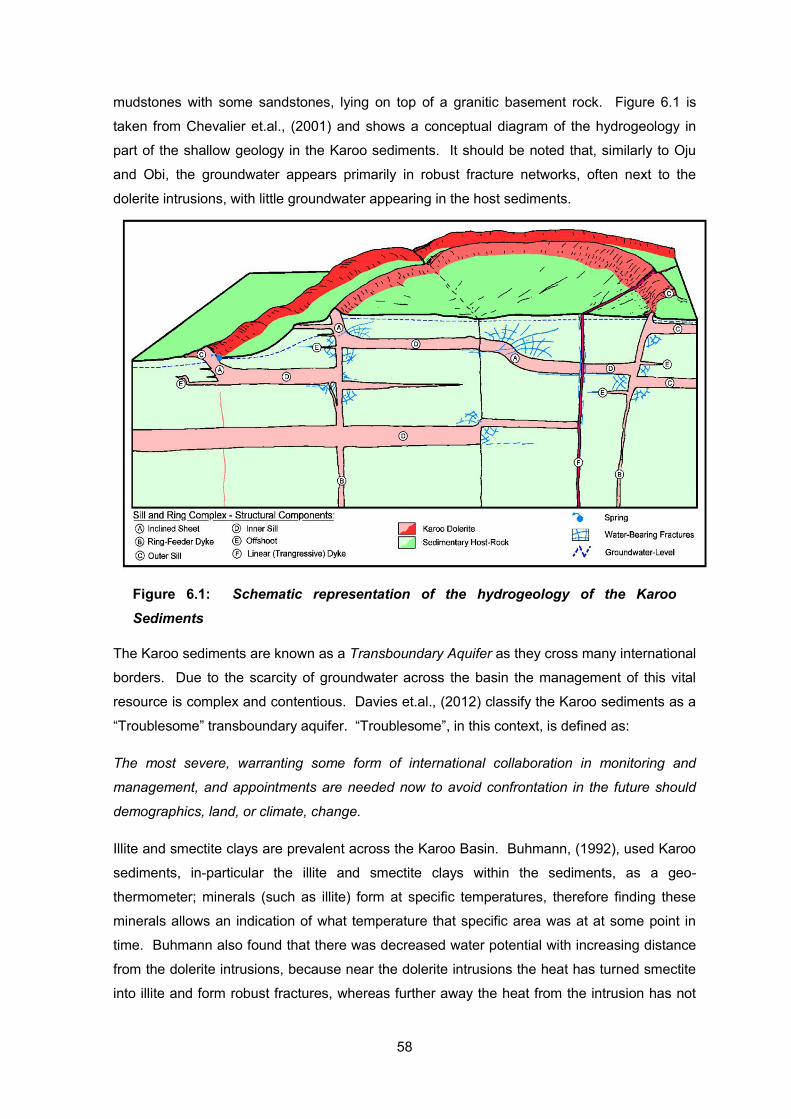
58

Figure 6.1: Schematic representation of the hydrogeology of the Karoo Sediments

mudstones with some sandstones, lying on top of a granitic basement rock. Figure 6.1 is

taken from Chevalier et.al., (2001) and shows a conceptual diagram of the hydrogeology in

part of the shallow geology in the Karoo sediments. It should be noted that, similarly to Oju

and Obi, the groundwater appears primarily in robust fracture networks, often next to the

dolerite intrusions, with little groundwater appearing in the host sediments.

The Karoo sediments are known as a Transboundary Aquifer as they cross many international

borders. Due to the scarcity of groundwater across the basin the management of this vital

resource is complex and contentious. Davies et.al., (2012) classify the Karoo sediments as a

“Troublesome” transboundary aquifer. “Troublesome”, in this context, is defined as:

The most severe, warranting some form of international collaboration in monitoring and

management, and appointments are needed now to avoid confrontation in the future should

demographics, land, or climate, change.

Illite and smectite clays are prevalent across the Karoo Basin. Buhmann, (1992), used Karoo

sediments, in-particular the illite and smectite clays within the sediments, as a geo-

thermometer; minerals (such as illite) form at specific temperatures, therefore finding these

minerals allows an indication of what temperature that specific area was at at some point in

time. Buhmann also found that there was decreased water potential with increasing distance

from the dolerite intrusions, because near the dolerite intrusions the heat has turned smectite

into illite and form robust fractures, whereas further away the heat from the intrusion has not

59

Figure 6.2: Geological map of the Karoo Basin

Table 6.1: Water demand, past and future, in the Karoo Basin

been significant enough to turn the smectite into illite. Figure 6.2 is taken from Buhmann,

(1992), and is a geological map of the different groups across the Great Karoo Basin; it is

good for highlighting the basin’s spatial extent.

The evidence which proves that groundwater is severely stressed in the region comes from

the paper by Le Maitre et.al., (2009). They state that in the driest areas of the plateau rainfall

is only 50-100mm per year. They go on to say that the water resources situation in Karoo (not

just groundwater) is approaching a crisis. Table 6.1 is an extract from their paper showing the

differences in availability and requirements for actual data from 2000 and for forecasted

predictions for 2025. What is clear is that for all catchments there is a water deficit. All values

are given in Mm3 yr-1.

60

Fortunately, the demand for domestic water in the region is quite low with the majority of the

demand coming from irrigation practices.

Many parallels can be drawn between this region and Oju & Obi in Nigeria. The hydrogeology

is essentially the same - no major aquifers, a groundwater scarce region, the presence of illite

and smectite, water filled fracture networks, dolerite intrusions, and increasing water potential

towards the dolerite intrusions and subordinate lithologies. It is clear that anyone who in the

future decides to undertake EM34 conductivity surveying within this region could use the

findings presented in this report to infer the locations of smectite and illite dominated areas by

analysing data from the vertical coil and assuming that high conductivities suggest smectite

abundance and low conductivities suggest illite abundance. Taking the findings of this report

into account could be the only way to dramatically increase drilling success rates and thus go

a considerable way to meeting the likely future demand.

The Voltaian Basin Sediments- Northern Ghana

Another region where the results of this project can be applied is in the water stressed region

of Northern Ghana. Compared to the Karoo Basin, there is comparably little information on

the hydrogeology of this particular area. It is speculated that the reason why far more

investigations have been gathered on the Karoo Basin is because of Shell’s interest in the

shale gas there. It is unlikely the South African government would grant drilling rights to Shell

before substantial fieldwork and mapping of the hydrogeology of the area had been

completed.

There are only really two major reports describing the hydrogeology of this region in question,

both of which have been compiled by the BGS. The report by O Dochartaigh et.al., (2011a),

describes how the BGS was commissioned to investigate low drilling success rates

encountered by UNICEF’s IWASH programme in Northern Ghana. The rocks in the region

form low-very low productivity aquifers with only minimal sustainable groundwater supplies

available. It is noted that the best target for groundwater is fracture networks within the

sandstone, with the mudstone having very little potential to yield any significant amounts of

groundwater. The mudstones are poorly fractured (suggesting mainly smectite dominated

clays). The findings of the BGS team showed that, as is often the case, geophysical surveying

is not being carried out correctly and it is not being used to its full potential. It was found that

the IWASH project did not use geophysics enough hence the poor siting of their boreholes.

This is a massive problem in the WATSAN sector. Airborne geophysics has taken place over

the region and a groundwater potential map has been produced. Figure 6.3 is this map; the

pink regions in the centre represent the best target for groundwater supply.

61

Figure 6.3: Airborne geophysics data of ground conductivity, Northern Ghana

A vast and comprehensive

description of the hydrogeology of

the area is given by O Dochartaigh

et.al., (2011b). To summarise, the

best groundwater targets are the

fractures within the sandstone; the

most important zone of

groundwater flow is 30-70m

beneath ground level; and there is

very little/no groundwater flow

beneath 100m depth.

The BGS have not published any

information regarding the clay

mineralogy of the area; therefore it

is not known what proportion of the

mudstone is smectite and what

proportion is illite. To solve this,

EM34 data could be collected

across the mudstones in the region

and areas of high conductivity

could be inferred as being smectite

and areas of low conductivity as

being illite. This would be

beneficial as the two previous

aforementioned reports state that

the mudstone is a poor target for

the groundwater, however, if the mudstones are illite dominated then robust fracture networks

may exist and boreholes/wells could be sited to provide plentiful, sustainable, and wholesome

rural water supplies.

The above two regions are areas in SSA where our findings could be put to good use to

increase success rates of striking groundwater in rural water stressed areas. It is easy to see

how the findings of this project can impact other water stressed areas as this dataset came

from a water stressed area; parallels can easily made and the significance can obviously be

appreciated. Whilst WATSAN is perhaps the area where this research has its most profound

significance, there are many other areas where the findings of this report have substantial

emphasis. These other fields of study are now discussed.

62

Identifying a Suitable Site for a High-Level Nuclear Waste

Repository

Whilst this topic does not fall under rural water supply it does fall under the umbrella of water

and environmental management and hydrogeology. One of the most crucial, important and

exciting topics in the field of engineering and environmental geology is where to site a

repository for highly radioactive nuclear waste. Highly radioactive nuclear waste originates

mainly from the decommissioning of nuclear sites, highly active and long lived waste products

from fuelling reactions, and also from other sites where radioactive isotopes are used - such

as hospitals. High-Level Waste (HLW) is particularly problematic as it will remain highly

radioactive for thousands to millions of years. Safe disposal of it requires not only

consideration of the health impacts for our generation but also the subsequent generations

after our own. Currently no disposal mechanism exists for the UK’s HLW and it is currently all

in storage in warehouses. This poses a problem as it is not a long term solution and it is a

good target for any terrorist threat. Many suggestions have been put forward as to how to

deal with the UK’s HLW, McKinley, (1992), summarises them well. Some examples of these

are as follows:

Send it to the sun - The sun offers permanent disposal as it is effectively a large

nuclear reactor itself. The downside is that rocket launch is risky; explosion of the

rocket would distribute vast quantities of lethal radioactive isotopes into the

atmosphere.

Indefinite storage - One option is to just leave the HLW in warehouses. This is not

really suitable though for reasons already mentioned.

Transmutation - Once considered the best option by many; transmutation involves

turning long lived radioactive isotopes into different, shorter-lived, and less dangerous,

radioactive isotopes. The problem with this idea though is that it involves significant

handling of the waste - something which is best avoided.

Bury it in the arctic ice caps - The heat produced by the radiation would melt the ice

and the waste would slowly sink deep beneath the ice caps and freeze over. There

are risks with climate change and it breaks international law.

Dump it in the sea - The waste product is off of land in the middle of the ocean.

Breaks the international marine dumping laws.

Place it in subduction zones - A subduction zone is an area where one tectonic

plate is being thrust beneath another deep into the earth’s mantle. Placing waste here

would push the waste deep beneath the crust. The issue is that it would take

thousands to millions of years for disposal.

Encapsulation in a very deep borehole - Drilling a deep borehole would allow you to

place the waste in the bottom of it. The heat from the radiation would melt the

63

surrounding rocks. After a few thousands of years when the activity has reduced the

rock would then cool and solidify around the waste thus trapping it within rock.

Difficulty arises with the technical aspects of drilling such a deep borehole.

All of the above suggestions have been seriously considered as a means of disposal. Whilst

nothing has officially been approved yet, the most likely means of disposal will be none of the

above, but burial in the ground in a nuclear waste repository. A nuclear waste repository must

meet the following criteria:

1. It must be sited in an area of low tectonic activity - Areas which are prone to high

tectonic activity are hotspots for earthquake activity. Earthquakes could rupture the

HLW repository and cause radioactive isotopes to enter the environment.

2. It must be sited in a hydrogeologically suitable formation - Radioactive isotopes

entering water allow the easiest and most rapid passage of movement throughout

underlying rock formations. It is essential that no water enters the repository.

Although waste will be encapsulated in barrels these will degrade over time and not

form a sturdy barrier. Therefore, a rock formation made of clay and minerals such as

anhydrite is needed to form a geological barrier to water flow.

3. It must be sited in a geologically ‘boring’ area - It is critical that the HLW is not

placed in an area of geological commercial interest. Putting it near to oil and gas

fields or rich mineral deposits will only encourage future generations to mine the area.

Stumbling across the repository could have lethal consequences for future miners and

the nearby communities.

What the reader should be able to appreciate is that the nuclear waste repository needs to be

sited in a ‘Goldilocks zone’, i.e. everything must be just right. Such spots are incredibly

difficult to locate and any information which leads to easier identification of potentially suitable

areas will be incredibly useful. The findings of this research project will help to identify a site

for HLW repositories.

The second criterion (in the list above) makes a sweeping generalisation that clay formations

are a good place to site HLW repositories. However, what this research and the findings of

many other scientists have shown is that illite clays allow significant groundwater flow.

Therefore, it is clear to see that one would not want to site one’s HLW repository in an illite

dominated area, nor would one want to site it in a smectite dominated area which is going to

be exposed to heat and pressure in the future thus facilitating the diagenetic transition of

turning smectite into illite. Pusch and Karnland, (1994), have studied how this transition of

smectite to illite will impact on HLW repositories; they state that when smectite turns into illite

it releases trapper interlayer water into the pore water spaces, further adding to groundwater

64

flow in the formation. Based on the likely geology of any suitable HLW repository site, they

even put a time limit on when this transition is likely to happen of several tens of thousands of

years. More work specifically related to smectite, illite and HLW repositories, showing that this

is a significant area of research, is the work by Hokmark et.al., (1997). They state that any

HLW repository is likely to include a clay buffer (clay will be added around the storage facility

in-between the barrels and the surrounding host rock) and they model how smectite will turn

into illite under these circumstances.

The research conducted for this area has explicitly shown that it is possible to distinguish

between illite and smectite dominated areas in the subsurface by taking surface conductivity

measurements. There is no reason why the findings of this research cannot be used in the

search of a suitable site for a HLW repository. Both time and money can be saved by

reducing the amount of boreholes and cores which will need to be drilled and gathered by

narrowing down the search area by identifying illite dominated areas in the subsurface using

ground conductivity data. Areas with high conductivities will suggest the presence of smectite

and therefore would be good areas to site HLW repositories. When the conductivity begins to

significantly drop, this would suggest illite/smectite and illite dominated regions which would

not be suitable due to the increased likelihood of increased fracture networks promoting

substantial fluid flow into and out of the repository. For this application, by some extension,

measured conductivity could be seen as being inversely proportional to the degree of risk to

public health and the environment.

Engineering Applications

One other area where the findings of this research could have implications is in the sector of

civil engineering and construction. Generally, engineers try to avoid building on clay as it is

often weak, plastic, and shears easily. Illite, being more robust and stronger, could perhaps

support some foundations if it is not overwhelmingly domineering. It is hypothesised that it

certainly would not be wise building on any smectite dominated formation due to its plastic

and deformable nature. Whilst the author would indeed like to bring civil engineering and

construction aspects into this report, it falls beyond the realm of this dissertation. Its

importance and appreciation is stressed, however no more is presented on the matter. Again,

the ability to use conductivity data to distinguish between different clay types in the subsurface

will have significant implications in this sector.

The above categories have provided a flavour as to which other sectors the findings of this

research could be applied to. Remote sensing is another area where this could be useful,

however this is discussed in more detail in the next chapter. What this chapter has provided

65

the reader with is an understanding of how this research is not just relevant to one particular

region, in one particular country, in one particular sector, but its significance can be

appreciated across many different sectors globally.

66

Figure 7.1: LANDSAT data taken over Greater London, UK

Chapter 7- The Next Steps

Presented in this report thus far has been a summary of work which has already been

completed many years ago by the BGS and the steps taken by the author to process the data

and turn it into something meaningful which has wider implications. The significance of the

research has already been presented in the previous chapter. With conclusions having been

drawn for the information presented in the subsequent chapters the next stage is to assess

what are the next steps? Where do we go from here? How can the research be furthered

both in the WATSAN sector and in other sectors? This chapter will highlight some suggested

next steps and suggestions for further study. Also, a summary of the research as a whole will

be presented and closing remarks will be made.

Suggestions for Further Study

Applications with Remote Sensing Data

The reason why this application is presented in this chapter and not in the previous one is

because it is not directly linked to the outcomes of this investigation. Linked to rural water

supply, but not exclusively dedicated to it, are the applications of this research which could be

applied to remote sensing data. There are, however, strong ties between the data which can

be collected by geophysical conductivity surveying methods and the data which can be

collected by remote sensing.

For the readers who are not

familiar with the topic, remote

sensing refers to the domain of

scientific information which can

be collected remotely, most often

referring to data collected by

satellite. LANDSAT is perhaps

the most famous example - it is a

satellite system which emits

electromagnetic radiation

towards the earth and measures

the degree of phase difference and interference in the reflected wave back to the satellite.

Figure 7.1 is an example of remote sensing data taken over London, United Kingdom, UCL,

(2013). This can tell us vast amounts of information about the nature of the ground surface

and can also provide strong clues as to the nature of the media making up the subsurface.

67

Naturally, the question should be asked as to whether or not remote sensing can successfully

come to the same conclusions about the nature of the subsurface as is drawn from our EM34

data used in this project. There are advantages to this because geophysical surveying is a

slow and expensive process to undertake; if the same information can be gathered via remote

sensing satellites then what usually takes months and many thousands of dollars to complete

could be completed in a matter of seconds and more often than not the data is free to obtain.

Short Literature Review on Remote Sensing Applications

Whilst it is beyond the scope of this research to actually process any remote sensing data, an

effort has been made to determine whether or not there is a strong possibility that remote

sensing can distinguish between smectite and illite clays on the surface and the subsurface.

Before going on to mention how remote sensing can be used to detect likely areas of

groundwater potential by mapping clay type it is worth mentioning that satellites are able to

detect groundwater via observing gravitational changes. Large scale gravity observations to

monitor groundwater changes have been undertaken, most notably by NASA with their

GRACE mission. GRACE measures the changes in orbit between two satellites depending

upon variations in gravity. Certain changes have been attributed to changing groundwater

levels. These have been particularly useful in measuring country-wide groundwater

variations, most notably in California, Texas, and India (NASA, 2012).

Kariuki et.al., (2003), used spectral data gathered by remote sensing satellites to estimate the

CEC of the ground (from which the clay type can be inferred). They noted that the spectral

range of 1300-2500nm was particularly good at being able to determine the CEC of the soil on

the surface. Other scientists have gone further by stating that remote sensing can directly

distinguish between smectite and illite.

Dogan, (2009), used remote sensing data to map distributions of illite and smectite in the

Kelkit River Basin in Turkey. Dogan realised that clay minerals are essential for productive

agriculture and therefore being able to rapidly distinguish between clay minerals and other

minerals is a substantial advantage in terms of both cost saving and time. Dogan states that

clay minerals are particularly susceptible to identification in the LANDSAT bands 5 and 7.

Van der Meer, (1999), presents a well-rounded comprehensive description on the uses of

remote sensing to identify clay mineralogy on the earth’s surface. Van der Meer highlights the

particular importance of being able to identify how clays swell. It is noted that swelling clays

pose a substantial geological hazard. When water is absorbed in-between clay plates they

become further separated; this destabilises the mineral structure and can present vast civil

engineering problems. Clays can swell up to 150% of their original size. It is noted that illite

has a lower swelling potential than smectite, therefore if one can measure the swell then one

can infer the clay type. It is noted that the swell could be measured by a system known as

68

InSAR which measures the changes in elevation of the earth’s surface. The problem with this

method, however, is that it is a temporal measurement, i.e. you need to take data over time to

see if the clay has swelled. Furthermore, just because a clay can swell does not necessarily

mean that it will, especially in water stressed regions such as Oju and Obi. Perhaps a more

logical approach in the context which we are focussing on would be to try and directly

measure the swell by analysing the reflectance properties of smectite and illite: something

which Van der Meer also suggests.

Kariuki et.al., (2004), present some of the advantages and disadvantages of using remote

sensing data to determine smectite or illite content. It is stated that recently the resolution of

the data has increased and therefore it is possible to identify the major mineral present in

every pixel of the image. Problems, however, include vegetation and free water cover which

mask any mineralogy beneath, and there are also problems when you have mixed clays in the

same area.

It is clear from the literature on this subject that it is possible to distinguish between different

clay types on the surface. What is also apparent is that remote sensing does not give a good

analysis of what can be found at depth, as it is primarily a tool which analyses reflectance -

which can only be used on exposed surfaces. Whilst many have focussed on the implications

of such research on civil engineering and more notably geohazards, there is no information

directly related to the aims of this research. This shows that there is work which could be

done by using remote sensing data over the Oju and Obi area and using the findings of this

research as something to compare it to.

Stronger Theoretical and Experimental Agreement

Chapter 5 proved that the agreement between theoretical predictions and experimental

evidence is at best inconclusive and at worst wrong. The issue is not that the models are

completely incorrect, more that they are based on laboratory measurements where specific

parameters can be identified; the field is a lot more variable and some of the parameters

cannot be measured but must be estimated from other information. As of yet, no one has

come up with a link which successfully describes how the microscopic behaviour of clays

manifests itself on a macroscopic level. The macroscopic level, however, is the most

important: especially in terms of locating suitable groundwater targets for rural water supply.

The results from this research show that the link between clay type and measured bulk

conductivity is linear when measured on a field-scale. As indicated in Chapter 5, however,

this may only be the case for when the surface conductivities and pore water conductivities

are similar. It is clear that further work on the theoretical side must be undertaken to enable

successful linear modelling of what is observed in the field.

69

A Comprehensive Survey of Water Supply in Oju and Obi Fifteen Years On

Personal conversation with Alan MacDonald of the BGS has provided some insight into how

the boreholes and wells constructed by the BGS are operating fifteen years on. MacDonald

states that to his knowledge the boreholes and wells are still, on the whole, operating

successfully and are still delivering clean, wholesome and sustainable water supplies in the

rural areas. He does indicate, however, that no comprehensive follow-up of the region has

been undertaken by the BGS to specifically quantify how well each of the boreholes/wells is

functioning. Naturally, some sort of region-wide survey would be prudent to conduct. It would

allow geological assessment of the ‘aquifers’, technical assessment of the hand-pumps and

wells, and the population’s satisfaction could be measured by means of a sociological survey.

This would enable us to categorically state whether or not the findings of this research would

be applicable and useful in the long-term. If by some geological process (such as weathering

or precipitation) the fractures in illite become blocked/filled over a very short period of time (in

geological terms) then illite fractures might not be the best targets for long-term, sustainable

rural water supplies. Whilst this is unlikely, it is possible.

Caution would have to be applied to the region-wide survey. If the boreholes and wells are

not yielding sufficient quantities of water, this may not be down to ‘aquifer’ degradation,

insufficient recharge, or water table draw-down; more often than not, these problems tend to

be more technical in nature with boreholes and hand-pumps not functioning as well due to

wear and tear of parts and overuse. These problems stem from more management related

issues and are arguably often more difficult to solve. If this turned out to be the case, drilling

of more boreholes would be pointless and a waste of money and resources.

Application of the Findings to Other Water Stressed Regions

Chapter 6 went into detail about where the findings of this research could be applied. From a

WATSAN perspective this is unquestionably the greatest use of this research. This research

will be of little use where there are an abundance of aquifers with substantial recharge. This

research will be of use in geologically unfavourable areas - where there is little aquifer

potential and poor recharge. In such areas, more so in areas which have a high population

like Oju and Obi, every drop of useable, accessible groundwater must be extracted to serve

the population (within sustainable limits, of course). Regions which have been written-off as

aquicludes can now be reinvestigated by knowing that illite fractures can produce sustainable

groundwater supplies, and that illite can be distinguished from smectite by using EM34

conductivity surveying as a linear relationship between clay type and conductivity has been

proven to exist.

If listened to, and acted upon, this research could vastly improve borehole siting success

rates. This would not only allow the best groundwater targets to be identified - by using the

70

horizontal coil to look for fracture networks and the vertical coil to tell you whether they are

likely to be illite or smectite based - but it would also save vast amounts of time, effort, and

crucially money. Many of the most water stressed regions in the world are often also some of

the poorest, and therefore any money which can be saved on siting boreholes can be put to

better use- such as lowering water tariffs and drilling more successful boreholes.

Summary of the Findings

In the previous chapters a robust description of the problem has been presented and

explained. Furthermore, solutions to the problem in question have been found and the

significance of the work has been described.

Chapter 1 provided a flavour of what the project was all about. Broader issues of African

hydrogeology, rural water supply, and geophysical surveying were presented. Chapter 2 very

much focussed on the birth of this project by describing in detail the work undertaken by the

BGS and where the data came from.

Once the problem had been clearly identified the literature review of clay and conductivity

enabled an appreciation to be gathered on the work which had already been published on the

topic. It became apparent that no one before had conducted any research to try and establish

a link between clay type and measured bulk conductivity on a macroscopic scale. This

justified the research being undertaken. The logical framework enabled a plan to be created

of the steps which needed to be completed whilst keeping in mind the overall goals which

wanted to be achieved.

The long and arduous process of sorting and processing the data was described step by step

in Chapter 4. Once values for conductivity and smectite content had been

calculated/estimated for the boreholes, the data points were able to be plotted onto graphs.

Both the gold-star and extended datasets yielded strong linear relationships with smectite

content of the subsurface being directly proportional to the measured bulk conductivity,

measured by the EM34 apparatus. This demonstrated that the conductance signal received

by the apparatus came mainly from the surface conductivity of the clays, not from the

conductivity of the freely mobile groundwater. Illite clays have the largest potential for creating

robust fracture networks- good groundwater targets- however due to its low CEC it produced a

comparatively small conductivity signal. This led to the groundbreaking conclusion that in such water-stressed clay dominated areas, geologists and geophysicists need to be looking for areas of low conductivity to have the best chance of finding groundwater. This fact is revolutionary as it goes completely against all other previous guiding principles which stated that areas of high conductivity signify groundwater flow in the subsurface. The last two sentences are written in bold to highlight their importance as the

71

take-home message from this research project. The implications of not knowing this counter-

intuitive fact, which this research has shown to be true, is proven by people in the Oju and Obi

region thinking that the Makurdi Sandstone formation was the best aquifer when in fact it was

one of the worst! As ever, what this research has shown is that things in geology, geophysics

and earth science are rarely so black and white as they may seem.

Who knows how many regions across the developing world have been surveyed and ruled out

as being clay aquifers with low conductivity, when really surveyors have actually stumbled

upon good illite fracture networks which make a good groundwater target? The beauty of this

research is that so long as the data for such regions still exist, further surveying need not take

place at the cost of both time and expense. Merely all that needs to be done is to look at the

data with a new eye, focussing on areas of low conductivity in the vertical coil signals and

using the horizontal coil signals to see whether robust fractures may be present.

As highlighted previously, the current models which try to describe the relationship between

clay and conductivity are inadequate. Either they focus too heavily on microscopic

parameters and thus they are not practical for using with field data (Revil and Glover’s model),

or they are likely to work with field data but only work when either the surface conductivity or

pore water conductivity is much greater than the other (Bussian’s model) which often, as in

the case of Oju and Obi, is not the case. The experimental data used in this research

suggests the relationship on a field-scale level is linear with increased smectite content

resulting in increased measured bulk conductivity.

Finally, the significance of the research and the suggestions for further study has been

discussed. As well as the obvious applications to the WATSAN sector, information on high

level nuclear waste repositories, engineering, geohazards and remote sensing have all been

mentioned. The findings of this research can be applied to many other sectors, making it a

worthwhile topic of study.

Closing Remarks

The past four months of research have enabled me to pursue my interest in hydrogeology and

rural water supply. I believe that the findings of this research could have significant and far-

reaching applications, especially in the WATSAN sector. Naturally, for the work to receive

wider recognition the findings must be summarised in journal format and published. I have

discussed this both with Ian Smout of WEDC, Loughborough University, and Alan MacDonald

of the BGS. Hopefully, someone with similar interests will be able to take this research further

and enable it to become useful in a practical way- a way which addresses some of the goals

mentioned in the logical framework in Chapter 3. This MSc dissertation has inspired me to

continue working in the field of research by undertaking a PhD in hydrogeology at the

72

University of Birmingham. This research has focussed heavily on finding groundwater in

regions where it is incredibly scarce, and as such I finish this dissertation with a quotation by

Antoine de Saint-Exupéry, a twentieth century, French writer, which summarises this research

and the topic of hydrogeology well:

“What makes the desert beautiful is that somewhere it hides a well.”

73

Acknowledgements

First and foremost, I would like to take this opportunity to thank my project supervisor at

WEDC, Ian Smout. His guidance, assistance, and enthusiasm for the project has enabled the

past four months of research to run smoothly and without any major difficulties. I would also

like to thank Alan MacDonald of the British Geological Survey. It was his idea that this project

would be a suitable and worthwhile topic of research to pursue. Furthermore, his assistance

both in person and via e-mail and telephone has been entirely voluntary and without his help

and guidance I could not have completed this research project. I would also like to extend my

gratitude to Mr Jonathan Pimperton (BSc Mathematical Sciences, University of Bath) who

assisted in solving one of the equations used in this report. Finally, I would like to thank Miss

Emily Wood who provided assistance with transportation and accommodation arrangements

on my frequent trips to Edinburgh to meet with Alan MacDonald at the British Geological

Survey’s Scottish Headquarters.

74

References

Adamson, A.W., 1982, Physical Chemistry of Surfaces, Wiley eds, ISBN: 978-0471148739

Archie, G.E., 1942, “The electrical resistivity log as an aid to determining some reservoir

characteristics”, Trans.Am. Inst. Mining Met. Eng., 146, 54-62

Bergaya. F., Langaly, G., 2006, “Chapter 1: General Introduction: Clays, Clay Minerals, &

Clay Science”, Developments in Clay Science 1. Handbook of Clay Science, (Edited by

Bergaya, F., Theng, B.K.G., Langaly, G.) Elsevier, Oxford, ISBN: 978-0-08-044183-2

Bergaya. F., Langaly, G.,Vayer. M., 2006, “Chapter 12: Cation and Anion Exchange”,

Developments in Clay Science 1. Handbook of Clay Science, (Edited by Bergaya, F., Theng,

B.K.G., Langaly, G.) Elsevier, Oxford, ISBN: 978-0-08-044183-2

Bromley, J., Mannstrom, B., Nisca, D., Jamtlid, A., 1994, “Airborne Geophysics: Application

to a groundwater study in Botswana”, Ground Water, Vol.34, pgs. 79-90

Buhmann, C., 1992, “Smectite-to-Illite Conversion in a Geothermally and Lithologically

Complex Permian Sedimentary Sequence”, Clays and Clay Minerals, Vol. 40, No. 1, pgs. 53-

64

Bussian, A.E., 1983, “Electrical conductance in a porous medium”, Geophysics, Vol. 48(9),

pgs. 1258-1268

Chevalier, L., Goedhart, M., Woodford, A.C., 2001, “The influence of dolerite sill and ring

complexes on the occurrence of groundwater in Karoo Fractured Aquifers: a morpho-tectonic

approach” WRC Report No. 937/1/01

Clavier, C., Coates, G., Dumanoir, J., 1977, “The theoretical and experimental bases for the

‘dual water’ model for the interpretation of shaly sands”, 52nd Ann. Fall Tech. Conf. and Exhib.

Soc. Petr. Eng. paper 6859

Davies, J., MacDonald, A.M., 1999, “Final Report: The groundwater potential of the Oju/Obi

area, Eastern Nigeria” British Geological Survey Technical Report, WC/99/32 Overseas

Geology Series, NERC

Davies, J., Robins, N.S., Farr, J., Sorenson, J., Beetlestone, P., Cobbing, J.E., 2012,

“Identifying transboundary aquifers in need of international resource management in the

SADC Region of southern Africa”, TBA Paper, British Geological Survey

75

de Lima, O.A.L., Sharma, M.M., 1990, “A grain conductivity approach to shaly sandstones”,

Geophysics, Volume 55, pgs. 1347-1358

Dogan, H.M., 2009, “Mineral composite assessment of Kelkit River Basin in Turkey by means

of remote sensing”, Journal of Earth Systems Science, Vol. 118, No. 6, pgs. 701-710

Encyclopaedia Britannica, No Author, Accessed Jul 2013, “Karoo System”,

http://www.britannica.com/EBchecked/topic/312642/Karoo-System

Federal Republic of Nigeria, 2013, “Benue State”, http://www.nigeria.gov.ng/2012-10-29-11-

06-21/north-central-states/benue-state, Accessed August 2013

Goes, M., 2012, “Karoo Groundwater Atlas: February 2012”, SRK Consulting (South Africa),

report prepared for Shell by SRK Consulting, Groundwater Africa, Prof G. Van Tonder, RPS

Aquaterra

Hokmark, H., Karnland, O., Pusch, R., 1997, “A technique for modelling

transport/conversion processes applied to smectite-to-illite conversion in HLW buffers”,

Engineering Geology, Vol. 47, pgs 367-378

Johnson, D.L., Sen, P.N., 1988, “Dependence of the conductivity of a porous medium on

electrolyte conductivity”, Phys. Rev, B, 37

Joint Monitoring Programme (JMP) for Water Supply and Sanitation, 2013a, “Population

with access to drinking water in 1990-2010”, WHO & UNICEF, http://www.wssinfo.org/data-

estimates/graphs/, accessed August 2013

Joint Monitoring Programme (JMP) for Water Supply and Sanitation, 2013b, “Percentage

of population with access to drinking water in Sub-Saharan Africa in 1990-2010”, WHO &

UNICEF, http://www.wssinfo.org/data-estimates/graphs/, accessed August 2013

Joint Monitoring Programme (JMP) for Water Supply and Sanitation, 2013c, “Population

with access to drinking water in Sub-Saharan Africa in 1990-2010”, WHO & UNICEF,

http://www.wssinfo.org/data-estimates/graphs/, accessed August 2013

Joint Monitoring Programme (JMP) for Water Supply and Sanitation, 2013d, “Nigeria:

estimates on the use of water sources and sanitation facilities (1980-2011)”, WHO & UNICEF,

http://www.wssinfo.org/documents-links/documents/?tx_displaycontroller[type]=country_files,

Accessed August 2013

Karikuki, P.C., Van Der Meer, F., Verhoef, P.N.W., 2003, “Cation Exchange Capacity (CEC)

determination from spectroscopy”, International Journal of Remote Sensing, Vol. 24, No. 1,

pgs. 161-167

76

Kariuki, P.C., Woldai, T., Van Der Meer, F., 2004, “Effectiveness of spectroscopy in

identification of swelling indicator clay minerals”, International Journal of Remote Sensing, Vol.

25, No. 2, pgs. 455-469

Kearey, P., Brooks, M., Hill, I., 2002, An introduction to geophysical exploration, Third

edition, Blackwell Publishing, Oxford, United Kingdom, ISBN: 978-0-632-04929-5

Le Maitre, D., Colvin, C., Maherry, A., 2009, “Water resources in the Klein Karoo: the

challenge of sustainable development in a water-scarce areas”, South African Journal of

Science, 105

MacDonald, A., 1999, “PhD Thesis”, BGS, contact author if copy is required. Not available in

the public domain

MacDonald, A.M., Davies, J., 1997, “The hydrogeology of the Oju area, Eastern Nigeria: an

initial assessment”, British Geological Survey Technical Report, WC/97/54 Overseas Geology

Series, NERC

MacDonald, A.M., Davies, J., 1998, “Groundwater development maps of Oju and Obi Local

Government Areas, Eastern Nigeria”, British Geological Survey Technical Report, WC/98/53

Overseas Geology Series, NERC

MacDonald, A.M., Davies, J., 2000, “A brief review of groundwater for rural water supply in

Sub-Saharan Africa”, BGS Technical Report WC/00/33, Overseas Geology Series

MacDonald, A.M., Davies, J., No Date, “Communicating groundwater research: the example

of Oju and Obi, eastern Nigeria”, British Geological Survey Technical Report, WC/00/07

Overseas Geology Series, NERC

MacDonald, A.M., Kemp, S.J., Davies, J., 2005, “Transmissivity Variations in Mudstones”,

Ground Water, Vol.43, No.2, pgs 259-269.

McKinley, I.G., 1992, “The management of long lived nuclear waste”, Energy Policy,

Butterworth-Heinemann Ltd

Merriman, R.J., Peacor, D.R., 1999, “Very low grade meta-pelites: mineralogy, microfabrics

and measuring reaction progress”, Low Grade Metamorphism, ed. M. Frey and D. Robinson,

10-60. Oxford: Blackwell Science

NASA, 2012, “GRACE mission”, http://www.nasa.gov/mission_pages/Grace/index.html

O Dochartaigh, B.E., Davies, J., Beamish, D., MacDonald, A.M., 2011a, “BGS

Consultancy: UNICEF IWASH Project, Northern Region, Ghana. Final Report”, BGS

Groundwater Science Programme, Open Report OR/11/017

77

O Dochartaigh, B.E., Davies, J., Beamish, D., MacDonald, A.M., 2011b, “UNICEF IWASH

Project, Northern Region, Ghana: An adapted training manual for groundwater development”,

BGS Groundwater Science Programme, Open Report OR/11/047

Price, M., 1996, Introducing Groundwater, Stanley Thornes (Publishers) Ltd, Second Edition,

pgs. 15, ISBN: 0-7487-4371-5

Pusch, R., Karnland, O., 1994, “Physico/chemical stability of smectite clays”, Engineering

Geology, Vol. 41, pgs 73-85

Revil, A., Glover, P.W.J., 1998, “Nature of surface electrical conductivity in natural sands,

sandstones, and clays”, Geophysical Research Letters, Volume 25, No.5, pgs. 691-694.

Ruffet, C., Darot, M., Gueguen, Y., 1995, “Surface conductivity in rocks: A review”, Surveys

in Geophysics, Volume 16, pgs. 83-105

Sansom, K., Reed, B., Shaw, R., 2011, “An introduction to the logical framework”, WEDC

Publication: Booklet 6, Loughborough University, ISBN: 9781 84380 14 6 7

Tabbagh, A., Cosenza, P., 2007, “Effect of microstructure on the electrical conductivity of

clay-rich systems”, Physics and Chemistry of the Earth, Volume 32, pgs. 154-160

UCL (University College London), Accessed 2013, “MSc Remote Sensing”,

http://www.geog.ucl.ac.uk/admissions-and-teaching/postgraduates/msc-remote-sensing

Van Der Meer, F., 1999, “Can we map swelling clays with remote sensing?”, JAG, Volume 1,

Issue 1, pgs. 27-35

WaterAid Nigeria, 2013, “What we do: The Crisis- Water”, http://www.wateraid.org/ng/what-

we-do/the-crisis/water, Accessed August 2013

WaterAid, 2013, “Statistics: The hard facts behind the crisis”,

http://www.wateraid.org/uk/what-we-do/the-crisis/statistics, accessed August 2013

Waxman, M.H., Smits, L.J.M., 1968, “Electrical conductivities in oil-bearing shaly sands”,

Soc. Petr. Eng. J., Vol. 8, pgs. 107-122

WEDC, 2012, “Groundwater- Water Source Development Notes- Unit 3- Lecture Notes”,

Loughborough University, pg. 9

Wilson, M.J., 1994, “Clay mineralogy: spectroscopic and chemical determinative methods”,

Chapman and Hall, London, ISBN: 9780412533808

78

APPENDICES

79

Appendix I – Hydrogeology Maps

80

81

Appendix II – Inventory of Data

EM CONDUCTIVITY (GREEN DOTS)

1. ADWTEM_1- Sheet 1, Sheet 2, Figures (Sheet 3), (6 degs 58.05, 8 degs 18.022) 2. Ijekwe- Sheet 1, Figures (Sheet 2), IJKWEM_1- Sheet 1 Village Ijekwe, Figures (Sheet 2),

(7 degs 01.371, 8 degs 13.629). 3. OHYEEM_1- Sheet 1 Village Ohuiye, Sheet 2, Figures (Sheet 3), (6 degs 56.944, 8 degs

11.46) 4. OCHING- Sheet 1: Village Ochinyini, Sheet 2, Sheet 3, 1-2 (Sheet 4,) 3-4 (Sheet 5),

diagram (Sheet 6), (7 degs 00.873, 8 degs 23.284) 5. ODBOEM_1- Sheet 1 Village Odubwo, Sheet 2, Figures (Sheet 3), OD1/2/3/4/7/8 (START

6 degs 52.27, 8 degs 29.87, FINISH 6 degs 87392, 8 degs 50473) 6. ODBOEM_1- OD5/6, ODBOEM_2- Sheet 1, Village Odubwo, Sheet 2, (START 6 degs

53.091, 8 degs 30.405) 7. ODBOEM_3- 9, 10, 11 (Sheet 1) (START 6 52.201 8 29.847, FINISH '6 52.388 8

29.963). 8. ODBOEM_3- 12, 13 (Sheet 2), (START '6 52.388 8 29.963, FINISH 6 52.63 8

30.06). 9. ODBOEM_3- 14, 15 (Sheet 3), (START 6 52.768 8 30.161, FINISH 6 52.876 8

30.212). 10. Wataid- WA 1 (Sheet 1), (Lat 6 degs 52.310 North, 8 degs 26.152' East). 11. EMOJOK1- Village Ojekwe, Sheet 2: Traverse 1 (START 6.7718 8.3249, FINISH 6.7744

8.3164). 12. EMOJOK1-Sheet 3: Traverse 2 (START 6.7696 8.325, FINISH 6.7668 8.3171). 13. EMOJOK1-Sheet 4: Traverse 3 (START 6.7702 8.3183, FINISH 6.7711 8.3125). 14. EMOJOK1-Sheet 5: Traverse 4, Sheet 9: Traverse 6, Sheet 10: Traverse 7 (START

6.7711 8.3125). 15. EMOJOK1-Sheet 6: Traverse 3/4 anisotropy test section. Sheet 8: Traverse 5 (START

6.77227 8.3252). 16. Adega- adega AD1 (Sheet 1), (7 degs 02.869, 8 degs 16.253). 17. AdumWest- AW1 (Sheet 1), (Sheet 3), Sheet 4, (6 degs 56.163, 8 degs 17.398) 18. AKIRIBA- 1-7 (Sheet 1): Village Akiraba-ainu (6 degs 52.400, 8 degs 21.743) 19. AMAKA- AM1 (Sheet 1): Village Amaka-Ijegwu, graphs (Sheet 2), (7 degs 05.409, 8

degs 17.040). 20. AMAKA-AM2 (Sheet 4), (7 degs 05.476; 8 degs 16.790). 21. ANYOGA- AE1 (Sheet 1): Village Anyoga Eddi Adum East, (6 degs 57.18; 8 degs

22.130). 22. ANYOGA-AE3-5 (Sheet 3): (6 degs 56.477' 8 degs 22.223). 23. EDUMAG- Village Edumoga, Conductivity (6 degs 53.406; 8 degs 22.422) 24. ITOGO- Village Itogo, EM34 conductivity (START 7 degs 02.059; 8 degs 21.011', FINISH

7 degs 06.025; 8 degs 22.168') 25. ODADEM- Village Odaleko Adiko, EM34 conductivity (6 degs 59.195 8 degs 22.312) 26. OLUYO- Village Oluywo, EM34 (7 degs 01.728' 8 degs 19.364) 27. OYINYI- Village Oyinyi Lyeche, EM34 conductivity (6 degs 48.811; 8 degs 26.930)

82

28. Ugbodum- Village Ugbodum, EM34 conductivity ('6 degs 58.248' 8 degs 18.084') ACTUALLY THE SAME AS 1!!!

MAGNETICS (BLUE DOTS)

1. ADWTEM_1- Sheet 1, Figures (Sheet 3), (6 degs 58.05, 8 degs 18.022) 2. ADWTMG_1: Sheet1 (6 degs 55.949, 8 degs 17.13) 3. Ijekwe- Sheet 1, Figures (Sheet 2), IJKWEM_1- Sheet 1 Village Ijekwe, Figures (Sheet

2), IJKWMG_1- Sheet 1, (7 degs 01.371, 8 degs 13.629). 4. OHYEEM_1- Sheet 1: Village Ohuiye , Sheet 2, Figures (Sheet 3), (6 degs 56.944, 8

degs 11.46) 5. OHYEMG_1- Sheet 1, Sheet 2, (6 degs 56.9454, 8 degs 11.46) 6. OCHING- Village Ochinyini, 1-2 (Sheet 4), 3-4 (Sheet 5), (7 degs 00.873, 8 degs 23.284) 7. OCHYMG_1- Sheet 1, Sheet 3, (7 degs 00.873, 8 degs 23.284). SAME AS 6! 8. OCHYMG_1- Sheet 2, (START 7 degs 00.439, 8 degs 24.053, FINISH 6 degs 59.818, 8

degs 25.878) 9. ODBOEM_1- Figures (Sheet 3), (OD1/2/3/4/7/8 START 6 degs 52.27, 8 degs 29.87) 10. ODBOEM_1- Figures (Sheet 3), (OD5/6 START 6 degs 53.091, 8 degs 30.405) 11. ODBOMG_1- Sheet 1, Sheet 2, (6 degs 52.27, 8 degs 29.87). SAME AS 9! 12. ODBOMG_2- Sheet 1, (8 degs 30.405, 6 degs 53.091) 13. ODBOMG_2- Sheet 2 (8 degs 29.87, 6 degs 52.27) SAME AS 9! 14. OJKWMG_1- Sheet 1, (6 degs 46.305, 8 degs 19.494). 15. OJKWMG_1- Sheet 3, (6 degs 49.175, 8 degs 19.502). 16. OJKWMG_2- Sheet 1, Sheet 2, (8 degs 19.095, 6 degs 46.210) 17. OJKWMG_2- Sheet 3 (8 degs 180955, 6 degs 46.314). 18. OJKWMG_2- Sheet 4, Sheet 5 (8 degs 18.747, 6 degs 46.268). 19. AKIRIBA- 1-7 (Sheet 1): Village Akiraba-ainu (6 degs 52.400, 8 degs 21.743) 20. AMAKA- magnetics (Sheet 3) (7 degs 05.409, 8 degs 17.040) 21. OLUYO- Village Oluywo (7 degs 01.728' 8 degs 19.364) 22. OYINYI- Village Oyinyi Lyeche (6 degs 48.811; 8 degs 26.930), 23. Ugbodum- Village Ugbodum ('6 degs 58.248' 8 degs 18.084')

VES RESISTIVITY (YELLOW DOTS)

1. ADWERS_1- Sheet 1, Sheet 2 (6 degs 58.060, 8 degs 17.976) 2. OCHING- VES (Sheet 7): 3 res surveys, Survey 1 (7 degs 0.754, 8 degs 23.313) 3. OCHING- Survey 2 (7 degs 00.615, 8 degs 23.666) 4. OCHING- Survey 3 (6 degs 59.958, 8 degs 25.499) 5. OCHYRS_1- Sheet 1 (7 degs 00.735, 8 degs 23.323). 6. OCHYRS_1- Sheet 2 (7 degs 00.652, 8 degs 23.641) 7. ODBOEM_3- VES (Sheet 5), (START 6 52.768 8 30.161, FINISH 6 52.876 8

30.212). 8. Wataid- VES 1 (Sheet 2), (Lat 6 degs 52.310 North, 8 degs 26.152' East). 9. OJKWRS_1- Sheet 1, Sheet 2, (6 degs 46.336, 8 degs 19.512) 10. Adega- adega VES (Sheet 2), (7 degs 02.869, 8 degs 16.253) 11. AdumWest- VES (Sheet 2), (6 degs 56.163, 8 degs 17.398) 12. AKIRIBA- Village Akiraba-ainu, VES (Sheet 2), (6 degs 52.400, 8 degs 21.743)

83

13. AMAKA- VES (Sheet 6), (7 degs 06.142; 8 degs 15.497) 14. ANYOGA- ves (Sheet 2), (6 degs 57.18; 8 degs 22.130) 15. EDUMAG- VES (6 degs 53.418; 8 degs 22.655) 16. EDUMAG- VES (6 degs 53.433; 8 degs 22.342) 17. EDUMAG- VES (6 degs 53.433; 8 degs 22.342) SAME AS 16! 18. ITOGO- Village Itogo, VES (7 degs 04.287' 8 degs 22.162) 19. ITOGO- Village Itogo, (7 degs 02.743; 8 degs 21.116) 20. ODADEM- Village Odaleko Adiko, VES (6 degs 59.214; 8 degs 22.361) 21. ODADEM- Village Odaleko Adiko, VES (6 degs 59.180; 8 degs 22.399) 22. Boreholes- BGS40, 23. Boreholes-BGS41, (6 degs 58.157, 8 degs 16.702) 24. Boreholes-BGS42, 25. Boreholes-BGS43, (6 degs 58.853, 8 degs 15.960) 26. Boreholes-BGS44, (6 degs 58.539, 8 degs 16.227) 27. Boreholes-BGS46 (7 degs 0.842, 8 degs 14.993)

84

Appendix III – Bussian Equation Derivation

85

Bo

reh

ole

Me

an d

ep

thFo

rmat

ion

K

aoli

nit

eIl

lite

Sme

ctit

eIl

liti

e/S

me

ctit

eIl

lite

%Sm

ect

ie %

Sme

ctit

eSm

ect

ite

TO

TAL

Sme

ctit

e in

Ro

ckG

eo

logy

41.

5U

pp

er

Eze

Aku

e82

180

00

00

00

Soil

42.

5U

pp

er

Eze

Aku

e76

240

00

00

00

Soil

43.

5U

pp

er

Eze

Aku

e39

40

5870

3017

.417

.48.

7C

lay

44.

5U

pp

er

Eze

Aku

e24

20

7459

4130

.34

30.3

415

.17

Cla

y

45.

5U

pp

er

Eze

Aku

e11

10

8861

3934

.32

34.3

217

.16

Cla

y- W

eat

he

red

Mu

dst

on

e

46.

5U

pp

er

Eze

Aku

e15

30

8263

3730

.34

30.3

415

.17

We

ath

ere

d M

ud

sto

ne

47.

5U

pp

er

Eze

Aku

e12

20

8659

4135

.26

35.2

617

.63

We

ath

ere

d M

ud

sto

ne

61.

5U

pp

er

Eze

Aku

385

057

5446

26.2

226

.22

13.1

1So

il

62.

5U

pp

er

Eze

Aku

254

071

5842

29.8

229

.82

14.9

1So

il/C

lay

63.

5U

pp

er

Eze

Aku

193

077

5842

32.3

432

.34

16.1

7C

lay

64.

5U

pp

er

Eze

Aku

144

082

5545

36.9

36.9

18.4

5W

eat

he

red

Mu

dst

on

e

65.

5U

pp

er

Eze

Aku

144

082

5050

4141

20.5

We

ath

ere

d M

ud

sto

ne

66.

5U

pp

er

Eze

Aku

164

080

5149

39.2

39.2

19.6

We

ath

ere

d M

ud

sto

ne

67.

5U

pp

er

Eze

Aku

133

083

4258

48.1

448

.14

24.0

7W

eat

he

red

Mu

dst

on

e

68.

5U

pp

er

Eze

Aku

94

087

5149

42.6

342

.63

21.3

15W

eat

he

red

Mu

dst

on

e

69.

5U

pp

er

Eze

Aku

136

081

6535

28.3

528

.35

14.1

75W

eat

he

red

Mu

dst

on

e

71.

5M

aku

rdi S

and

sto

ne

8614

00

72.

5M

aku

rdi S

and

sto

ne

8218

00

73.

5M

aku

rdi S

and

sto

ne

6436

00

74.

5M

aku

rdi S

and

sto

ne

5248

00

75.

5M

aku

rdi S

and

sto

ne

4555

00

81.

5M

aku

rdi S

and

sto

ne

8416

00

00

00

0So

il

82.

5M

aku

rdi S

and

sto

ne

8911

00

00

00

0So

il

83.

5M

aku

rdi S

and

sto

ne

668

026

5347

12.2

212

.22

6.11

Cla

y

84.

5M

aku

rdi S

and

sto

ne

296

065

5941

26.6

526

.65

13.3

25C

lay

85.

5M

aku

rdi S

and

sto

ne

255

071

4753

37.6

337

.63

18.8

15C

lay

86.

5M

aku

rdi S

and

sto

ne

212

077

5545

34.6

534

.65

17.3

25C

lay

87.

5M

aku

rdi S

and

sto

ne

335

062

6634

21.0

821

.08

10.5

4C

lay

88.

5M

aku

rdi S

and

sto

ne

264

070

6337

25.9

25.9

12.9

5C

lay

Appendix IV – Excel Spreadsheets

Clay Mineralogy

86

Bo

reh

ole

Me

an d

ep

thFo

rmat

ion

K

aoli

nit

eIl

lite

Sme

ctit

eIl

liti

e/S

me

ctit

eIl

lite

%Sm

ect

ie %

Sme

ctit

eSm

ect

ite

TO

TAL

Sme

ctit

e in

Ro

ckG

eo

logy

131.

5M

aku

rdi S

and

sto

ne

6634

00

00

0So

il

132.

5M

aku

rdi S

and

sto

ne

5644

00

00

0So

il

133.

5M

aku

rdi S

and

sto

ne

4251

70

07

3.5

Cla

y

134.

5M

aku

rdi S

and

sto

ne

3953

90

09

4.5

Cla

y

151.

5Lo

we

r Ez

e A

ku39

290

3260

4012

.812

.86.

4Fe

rric

rete

152.

5Lo

we

r Ez

e A

ku37

60

5763

3721

.09

21.0

910

.545

Ferr

icre

te

153.

5Lo

we

r Ez

e A

ku29

40

6767

3322

.11

22.1

111

.055

Ferr

icre

te/C

lay

154.

5Lo

we

r Ez

e A

ku23

30

7468

3223

.68

23.6

811

.84

Cla

y

155.

5Lo

we

r Ez

e A

ku17

30

8070

3024

2412

Cla

y

156.

5Lo

we

r Ez

e A

ku11

40

8574

2622

.122

.111

.05

Cla

y

157.

5Lo

we

r Ez

e A

ku9

10

9072

2825

.225

.212

.6C

lay/

We

ath

ere

d M

ud

sto

ne

158.

5Lo

we

r Ez

e A

ku8

30

8971

2925

.81

25.8

112

.905

We

ath

ere

d M

ud

sto

ne

159.

5Lo

we

r Ez

e A

ku6

30

9274

2623

.92

23.9

211

.96

We

ath

ere

d M

ud

sto

ne

161.

5Lo

we

r Ez

e A

ku64

360

00

00

00

Ferr

icre

te

162.

5Lo

we

r Ez

e A

ku66

340

00

00

0Fe

rric

rete

163.

5Lo

we

r Ez

e A

ku32

100

5871

2916

.82

16.8

28.

41Fe

rric

rete

164.

5Lo

we

r Ez

e A

ku20

70

7375

2518

.25

18.2

59.

125

Cla

y

165.

5Lo

we

r Ez

e A

ku10

40

8672

2824

.08

24.0

812

.04

Cla

y/W

eat

he

red

Mu

dst

on

e

166.

5Lo

we

r Ez

e A

ku1

70

9279

2119

.32

19.3

29.

66W

eat

he

red

Mu

dst

on

e

167.

5Lo

we

r Ez

e A

ku1

70

9170

3027

.327

.313

.65

We

ath

ere

d M

ud

sto

ne

168.

5Lo

we

r Ez

e A

ku1

60

9480

2018

.818

.89.

4W

eat

he

red

Mu

dst

on

e

169.

5Lo

we

r Ez

e A

ku1

60

9379

2119

.53

19.5

39.

765

We

ath

ere

d M

ud

sto

ne

181.

5Lo

we

r Ez

e A

ku65

350

00

00

00

Ferr

icre

te

182.

5Lo

we

r Ez

e A

ku25

70

6864

3624

.48

24.4

812

.24

Ferr

icre

te

183.

5Lo

we

r Ez

e A

ku17

50

7867

3325

.74

25.7

412

.87

Cla

y

184.

5Lo

we

r Ez

e A

ku14

60

8078

2217

.617

.68.

8C

lay

185.

5Lo

we

r Ez

e A

ku12

70

8270

3024

.624

.612

.3W

eat

he

red

Mu

dst

on

e

186.

5Lo

we

r Ez

e A

ku8

60

8674

2622

.36

22.3

611

.18

We

ath

ere

d M

ud

sto

ne

187.

5Lo

we

r Ez

e A

ku7

50

8867

3329

.04

29.0

414

.52

We

ath

ere

d M

ud

sto

ne

188.

5Lo

we

r Ez

e A

ku15

70

7869

3124

.18

24.1

812

.09

We

ath

ere

d M

ud

sto

ne

189.

5Lo

we

r Ez

e A

ku12

60

8266

3427

.88

27.8

813

.94

We

ath

ere

d M

ud

sto

ne

87

Bo

reh

ole

Me

an d

ep

thFo

rmat

ion

K

aoli

nit

eIl

lite

Sme

ctit

eIl

liti

e/S

me

ctit

eIl

lite

%Sm

ect

ie %

Sme

ctit

eSm

ect

ite

TO

TAL

Sme

ctit

e in

Ro

ckG

eo

logy

191.

5A

su R

ive

r58

420

00

00

Soil

192.

5A

su R

ive

r63

325

00

52.

5C

lay

193.

5A

su R

ive

r55

396

00

63

Cla

y

194.

5A

su R

ive

r48

475

00

52.

5W

eat

he

red

Mu

dst

on

e

195.

5A

su R

ive

r36

577

00

73.

5W

eat

he

red

Mu

dst

on

e

196.

5A

su R

ive

r48

4011

00

115.

5W

eat

he

red

Mu

dst

on

e

197.

5A

su R

ive

r34

5611

00

115.

5W

eat

he

red

Mu

dst

on

e

198.

5A

su R

ive

r38

4913

00

136.

5D

ole

rite

211.

5A

su R

ive

r51

490

00

00

Soil

212.

5A

su R

ive

r46

540

00

00

Soil

/Cla

y

213.

5A

su R

ive

r37

4716

00

168

Cla

y

214.

5A

su R

ive

r30

655

00

52.

5W

eat

he

red

Mu

dst

on

e

2714

.5A

wgu

Sh

ale

s36

360

00

6030

Lim

est

on

e

2719

.5A

wgu

Sh

ale

s35

363

00

6331

.5Li

me

sto

ne

301.

5A

wgu

Sh

ale

s57

439

00

3919

.5So

il

302.

5A

wgu

Sh

ale

s44

452

00

5226

Cla

y

303.

5A

wgu

Sh

ale

s35

362

00

6231

Cla

y

304.

5A

wgu

Sh

ale

s42

553

00

5326

.5C

lay/

Fin

e G

rain

ed

San

d

305.

5A

wgu

Sh

ale

s41

355

00

5527

.5Fi

ne

Gra

ine

d S

and

306.

5A

wgu

Sh

ale

s31

267

00

6733

.5Fi

ne

Gra

ine

d S

and

307.

5A

wgu

Sh

ale

s34

462

00

6231

We

ath

ere

d S

and

sto

ne

308.

5A

wgu

Sh

ale

s23

374

00

7437

We

ath

ere

d S

and

sto

ne

309.

5A

wgu

Sh

ale

s37

360

00

6030

We

ath

ere

d S

and

sto

ne

3010

.5A

wgu

Sh

ale

s32

464

00

6432

Mu

dst

on

e

88

Bo

reh

ole

Me

an d

ep

thFo

rmat

ion

K

aoli

nit

eIl

lite

Sme

ctit

eIl

liti

e/S

me

ctit

eIl

lite

%Sm

ect

ie %

Sme

ctit

eSm

ect

ite

TO

TAL

Sme

ctit

e in

Ro

ckG

eo

logy

311.

75A

wgu

Sh

ale

s56

539

00

3919

.5So

il

312.

25A

wgu

Sh

ale

s35

164

00

6432

Soil

312.

75A

wgu

Sh

ale

s44

254

00

5427

Soil

/Cla

y

313.

25A

wgu

Sh

ale

s37

162

00

6231

Cla

y

313.

75A

wgu

Sh

ale

s32

068

00

6834

Cla

y

314.

25A

wgu

Sh

ale

s34

363

00

6331

.5C

lay

314.

75A

wgu

Sh

ale

s26

173

00

7336

.5C

lay

315.

25A

wgu

Sh

ale

s23

176

00

7638

Cla

y

321.

5A

wgu

Sh

ale

s49

051

00

5125

.5

322.

5A

wgu

Sh

ale

s35

164

00

6432

323.

5A

wgu

Sh

ale

s43

453

00

5326

.5

324.

5A

wgu

Sh

ale

s38

2141

00

4120

.5

325.

5A

wgu

Sh

ale

s32

167

00

6733

.5

3210

.5A

wgu

Sh

ale

s31

267

00

6733

.5

341.

5A

wgu

Sh

ale

s3

10

9655

4543

.243

.221

.6So

il/C

lay

342.

5A

wgu

Sh

ale

s2

20

9651

4947

.04

47.0

423

.52

Cla

y

343.

5A

wgu

Sh

ale

s5

50

9060

4036

3618

Cla

y

344.

5A

wgu

Sh

ale

s4

20

9470

3028

.228

.214

.1C

lay/

We

ath

ere

d M

ud

sto

ne

348.

5A

wgu

Sh

ale

s1

210

7860

4031

.231

.215

.6W

eat

he

red

Mu

dst

on

e

3429

.5A

wgu

Sh

ale

s31

160

5358

4222

.26

22.2

611

.13

Mu

dst

on

e

3430

.5A

wgu

Sh

ale

s32

10

6765

3523

.45

23.4

511

.725

Mu

dst

on

e

3431

.5A

wgu

Sh

ale

s13

027

6067

3319

.846

.823

.4M

ud

sto

ne

351.

5D

ole

rite

790

210

2110

.5So

il

352.

5D

ole

rite

370

630

6331

.5So

il

353.

5D

ole

rite

270

730

7336

.5C

lay

354.

5D

ole

rite

80

920

9246

Cla

y

355.

5D

ole

rite

40

960

9648

We

ath

ere

d D

ole

rite

356.

5D

ole

rite

10

990

9949

.5W

eat

he

red

Do

leri

te

357.

5D

ole

rite

00

100

010

050

We

ath

ere

d D

ole

rite

361.

5M

aku

rdi S

and

sto

ne

4456

00

00

00

0So

il

363.

5M

aku

rdi S

and

sto

ne

160

084

8911

9.24

9.24

4.62

Cla

y

365.

5M

aku

rdi S

and

sto

ne

90

091

8119

17.2

917

.29

8.64

5W

eat

he

red

San

dto

ne

89

Smectite and Conductivity Table

Borehole Conductivity Smectite Formation

19 4.71 3.63 Metamorphosed Asu River

21 19.01 2.63 Metamorphosed Asu River

1 8.13 5.5 Asu River

2 14 7 Asu River

17 35.23 8.91 Lower Eze Aku

18 34.7 10.88 Lower Eze Aku

15 33.26 11.15 Lower Eze Aku

16 34 8.01 Lower Eze Aku

14 30.92 9.53 Lower Eze Aku

22 110.08 31.2 Awgu Shale

28 100 29.89 Awgu Shale

26 113.11 29.6 Awgu Shale

25 136.83 28.11 Awgu Shale

24 126.13 30.06 Awgu Shale

23 94.05 30.45 Awgu Shale

27 95.19 30.75 Awgu Shale

30 85.28 29.4 Awgu Shale

31 107.42 31.19 Awgu Shale

34 72.18 17.38 Awgu Shale/ Dolerite

33 39.03 19.1 Awgu Shale/ Dolerite

4 50.78 10.55 Upper Eze Aku

6 87.93 18.03 Upper Eze Aku

5 49.01 12.58 Upper Eze Aku

9 15.65 2.18 Makurdi Sandstone

10 21.84 9.43 Makurdi Sandstone

11 13.52 2.18 Makurdi Sandstone

12 14 6.44 Makurdi Sandstone

37 16.39 7.81 Makurdi Sandstone

38 26.78 6.08 Makurdi Sandstone

7 16.22 0 Makurdi Sandstone

8 29.85 9.88 Makurdi Sandstone

36 16.39 4.42 Makurdi Sandstone

90

Groundwater quality - Conductivity of Pore Water

Borehole Conductivity mS/m

2 45.7

4 41

6 122.5

7 54.5

8 39.9

10 55.3

12 40.5

13 647

15 58.3

16 55.8

17 114.9

19 53.2

20 69.9

21 58.8

26 1008

27 716

30 20.1

33 50.9

34 51.8

35 54.6

36 151

37 96.5

39 52.1

40 61.4

41 250

42 56.3

44 41.7

46 31.6

48 499

50 55.8

13a 51.3

2b 45.4

91

Revil and Glover, and Experimental Conductivities

Borehole Conductivity Experiment Conductivity Model

4 50.78 25.73613536

6 87.93 66.64516053

7 16.22 23.2937653

8 29.85 24.74699515

15 33.26 34.7944315

16 34 32.21320374

19 4.71 27.52932686

21 19.01 29.28767706

30 85.28 15.54247124

34 72.18 33.70223931

36 16.39 65.05015707

27 95.19 284.2676322