1

Classical and Bayesian Inference in fMRI

William D. Penny and Karl J. Friston

The Wellcome Department of Imaging Neuroscience,

University College London

Queen Square, London, UK WC1N 3BG

Tel (44) 020 7833 7478

Fax (44) 020 7813 1420

Email: w.penny@fil.ion.ucl.ac.uk

Contents

1 Introduction

2 Spatial transformations

3 General linear modelling

4 Statistical parametric mapping

5 Posterior probability mapping

6 Dynamic causal modelling

7 Conclusion

References

2

1. INTRODUCTION

A general issue in the analysis of fMRI data is the relationship between the neurobiological

hypothesis one posits and the statistical models adopted to test that hypothesis. One key

distinction is between functional specialization and integration. Briefly, fMRI was originally

used to provide functional maps showing which regions are specialised for specific functions,

a classic example being the study by Zeki et al. (1991) who identified V4 and V5 as being

specialised for the processing of colour and motion, respectively. More recently, these

analyses have been augmented by functional integration studies, which describe how

functionally specialised areas interact and how these interactions depend on changes of

context. A recent example is the study by Buchel et al. (1999) who found that the success

with which a subject learned an object-location association task was correlated with the

coupling between regions in the dorsal and ventral visual streams (Ungerleider and Mishkin,

1982). In this chapter, we will address the design and analysis of neuroimaging studies from

these two distinct perspectives but note that they have to be combined for a full

understanding of brain mapping results.

In practice, the General Linear Model (GLM) is used to identify functionally specialized

brain responses and is the most prevalent approach to characterizing functional anatomy and

disease-related changes. GLMs are fitted to fMRI time series at each voxel resulting in a set

of voxel specific parameters. These parameters are then used to form Statistical Parametric

Maps (SPMs) or Posterior Probability Maps (PPMs) that characterise regionally specific

responses to experimental manipulation. Figures 4 and 5, for example, show SPMs and

PPMs highlighting regions that are sensitive to visual motion stimuli.

Analyses of functional integration are implemented using multivariate approaches

that examine the changes in multiple brain areas induced by experimental manipulation.

3

Although there a number of methods for doing this we focus on a recent approach called

Dynamic Causal Modelling (DCM).

In order to assign an observed response to a particular brain structure, or cortical area,

the data must conform to a known anatomical space. Before considering statistical modeling,

this chapter therefore deals briefly with how a time-series of images (from single or multiple

subjects) are realigned and mapped into some standard anatomical space (e.g. a stereotactic

space).

A central issue in this chapter is the distinction between Classical and Bayesian

estimation and inference. Historically, the most popular and successful method for the

analysis of fMRI is SPM. This is based on voxel-wise general linear modelling and Gaussian

Random Field (GRF) theory. More recently, a number of Bayesian estimation and inference

procedures have appeared in the literature. A key reason behind this is that, as our models

become more realistic (and therefore complex) they need to be constrained in some way. A

simple and principled way of doing this is to use priors in a Bayesian context. In this chapter

we will see Bayesian methods being used in spatial normalisation (section 2.3), posterior

probability mapping (section 5) and dynamic causal modelling (section 6). One should not

lose sight, however, of the simplicity of the original SPM procedures (section 4) as they

remain attractive both from an interpretive and computational perspective.

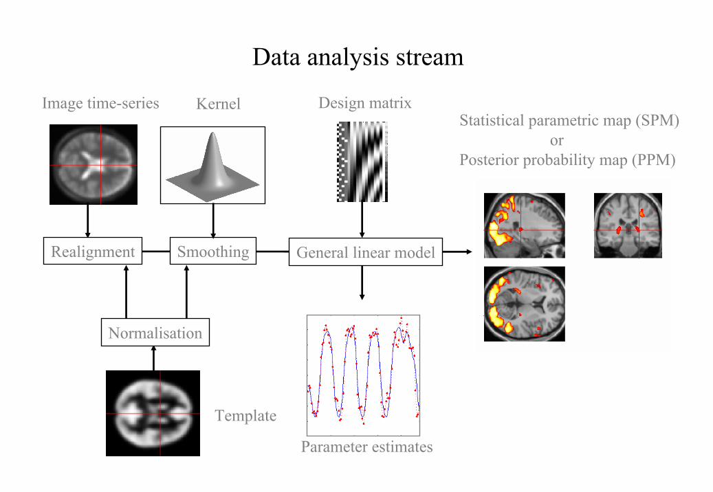
The analysis of functional neuroimaging data involves many steps that can be broadly

divided into; (i) spatial processing, (ii) estimating the parameters of a statistical model and

(iii) making inferences about those parameter estimates with appropriate statistics. This data

processing stream is shown in Figure 1.

4

2. SPATIAL TRANSFORMATIONS

The analysis of neuroimaging data generally starts with a series of spatial transformations.

These transformations aim to reduce unwanted variance components in the voxel time-series

that are induced by movement or shape differences among a series of scans. Subsequent

analyses assume that the data from a particular voxel all derive from the same part of the

brain. Violations of this assumption will introduce artifactual changes in the voxel values

that may obscure changes, or differences, of interest. Even single-subject analyses proceed

in a standard anatomical space, simply to enable reporting of regionally-specific effects in a

frame of reference that can be related to other studies.

The first step is to realign the data to 'undo' the effects of subject movement during the

scanning session. After realignment the data are then transformed using linear or nonlinear

warps into a standard anatomical space. Finally, the data are usually smoothed spatially prior

to analysis with a general linear model.

2.1 Realignment

Changes in signal intensity over time, from any one voxel, can arise from head motion and

this represents a serious confound for fMRI studies. Despite physical restraints on head

movement, subjects can still show displacements of up several millimeters. Realignment

involves (i) estimating the 6 parameters of an affine 'rigid-body' transformation that minimize

the [sum of squared] differences between each successive scan and a reference scan (usually

the first or the average of all scans in the time series) and (ii) applying the transformation by

re-sampling the data using tri-linear, sinc or spline interpolation. Estimation of the affine

transformation is usually effected with a first order approximation of the Taylor expansion of

5

the effect of movement on signal intensity using the spatial derivatives of the images (see

below). This allows for a simple iterative least square solution that corresponds to a Gauss-

Newton search (Friston et al 1995a). Even if this realignment were perfect, other movement-

related signals (see below) could still persist. This calls for a further step in which the data

are adjusted for residual movement-related effects.

2.2 Adjusting for movement related effects in fMRI

In extreme cases as much as 90% of the variance, in fMRI time-series, can be accounted for

by the effects of movement even after realignment (Friston et al 1996a). Causes of these

movement-related components are due to movement effects that cannot be modeled using a

linear affine model. These nonlinear effects include; (i) subject movement between slice

acquisition, (ii) interpolation artifacts (Grootoonk et al 2000), (iii) nonlinear distortion due

to magnetic field inhomogeneities (Andersson et al 2001) and (iv) spin-excitation history

effects (Friston et al 1996a). The latter can be pronounced if the TR (repetition time)

approaches T1 making the current signal a function of movement history. These multiple

effects render the movement-related signal (y) a nonlinear function of displacement (x) in the

nth and previous scans ),,( 1 …−= nnn xxfy . By assuming a sensible form for this function, its

parameters can be estimated using the observed time-series and the estimated movement

parameters x from the realignment procedure. The estimated movement-related signal is then

simply subtracted from the original data. This adjustment can be carried out as a pre-

processing step or embodied in model estimation during the general linear model analysis.

The form for ƒ(x), proposed in Friston et al (1996a), was a nonlinear auto-regression model

that used polynomial expansions to second order. This model was motivated by spin-

excitation history effects and allowed displacement in previous scans to explain the current

movement-related signal. However, it is also a reasonable model for many other sources of

6

movement-related confounds. Generally, for TRs of several seconds, interpolation artifacts

supersede (Grootoonk et al 2000) and first order terms, comprising an expansion of the

current displacement in terms of periodic basis functions, are sufficient.

2.3 Normalization

After realigning the data, a mean image of the series, or other co-registered (e.g. a T1-

weighted) image, is used to estimate some warping parameters that map it onto a template

that already conforms to some standard anatomical space (e.g. Talairach and Tournoux

1988). This estimation can use a variety of models for the mapping, including: (i) a 12-

parameter affine transformation, where the parameters constitute a spatial transformation

matrix, (ii) low frequency spatial basis functions (usually a discrete cosine set or

polynomials), where the parameters are the coefficients of the basis functions employed and

(ii) a vector field specifying the mapping for each control point (e.g. voxel). In the latter

case, the parameters are vast in number and constitute a vector field that is bigger than the

image itself. Estimation of the parameters of all these models can be accommodated in a

simple Bayesian framework, in which one is trying to find the deformation parameters θ that

have the maximum posterior probability )|( yp θ given the data y, where

)()|()()|( θθθ pypypyp = . Put simply, one wants to find the deformation that is most

likely given the data. This deformation can be found by maximizing the probability of

getting the data, assuming the current estimate of the deformation is true, times the

probability of that estimate being true. In practice the deformation is updated iteratively

using a Gauss-Newton scheme to maximize )|( yp θ . This involves jointly minimizing the

likelihood and prior potentials ( | ) ln ( | )H y p yθ θ= − and ( ) ln ( )H pθ θ= − . The likelihood

potential is generally taken to be the sum of squared differences between the template and

deformed image and reflects the probability of actually getting that image if the

7

transformation was correct. The prior potential can be used to incorporate prior information

about the likelihood of a given warp. Priors can be determined empirically or motivated by

constraints on the mappings. Priors play a more essential role as the number of parameters

specifying the mapping increases and are central to high dimensional warping schemes

(Ashburner et al 1997).

In practice most people use an affine or spatial basis function warps and iterative least

squares to minimize the posterior potential. A nice extension of this approach is that the

likelihood potential can be refined and taken as the difference between the index image and

the best [linear] combination of templates (e.g. depicting gray, white, CSF and skull tissue

partitions). This models intensity differences that are unrelated to registration differences

and allows different modalities to be co-registered (see Figure 2).

2.4 Co-registration of functional and anatomical data

It is sometimes useful to co-register functional and anatomical images. However, with echo-

planar imaging, geometric distortions of T2* images, relative to anatomical T1-weighted data,

are a particularly serious problem because of the very low frequency per point in the phase

encoding direction. Typically for echo-planar fMRI magnetic field inhomogeneity, sufficient

to cause dephasing of 2π through the slice, corresponds to an in-plane distortion of a voxel.

'Unwarping' schemes have been proposed to correct for the distortion effects (Jezzard and

Balaban 1995). However, this distortion is not an issue if one spatially normalizes the

functional data.

2.5 Spatial smoothing

The motivations for smoothing the data are fourfold. (i) By the matched filter theorem, the

optimum smoothing kernel corresponds to the size of the effect that one anticipates. The

8

spatial scale of hemodynamic responses is, according to high-resolution optical imaging

experiments, about 2 to 5mm. Despite the potentially high resolution afforded by fMRI an

equivalent smoothing is suggested for most applications. (ii) By the central limit theorem,

smoothing the data will render the errors more normal in their distribution and ensure the

validity of inferences based on parametric tests. (iii) When making inferences about regional

effects using Gaussian random field theory (see below) the assumption is that the error terms

are a reasonable lattice representation of an underlying and smooth Gaussian field. This

necessitates smoothness to be substantially greater than voxel size. If the voxels are large,

then they can be reduced by sub-sampling the data and smoothing (with the original point

spread function) with little loss of intrinsic resolution. (iv) In the context of inter-subject

averaging it is often necessary to smooth more (e.g. 8 to 12 mm) to project the data onto a

spatial scale where homologies in functional anatomy are expressed among subjects.

3 THE GENERAL LINEAR MODEL Statistical analysis of fMRI data entails (i) modeling the data to partition observed

neurophysiological responses into components of interest, confounds and error and (ii)

making inferences about the interesting effects in relation to the error variance. This can be

regarded as a direct comparison of the variance attributable to an interesting experimental

manipulation to the variance attributable to the error. These comparisons can be made with T

or F statistics.

A brief review of the literature may give the impression that there are numerous ways to

analyze fMRI time-series with a diversity of statistical and conceptual approaches. This is,

however, not the case. With few exceptions, every analysis is a variant of the general linear

model. This includes; (i) simple T tests on scans assigned to one condition or another, (ii)

9

correlation coefficients between observed responses and boxcar stimulus functions in fMRI,

(iii) inferences made using multiple linear regression, (iv) evoked responses estimated using

linear time invariant models and (v) selective averaging to estimate event-related responses.

Mathematically, they are formally identical and can be implemented with the same equations

and algorithms. The only thing that distinguishes among them is the design matrix encoding

the experimental design. The use of the correlation coefficient deserves special mention

because of its popularity in fMRI (Bandettini et al 1993). The significance of a correlation is

identical to the significance of the equivalent T statistic testing for a regression of the data on

the stimulus function. The correlation coefficient approach is useful but the inference is

effectively based on a limiting case of multiple linear regression that obtains when there is

only one regressor. In fMRI many regressors usually enter into a statistical model.

Therefore, the T statistic provides a more versatile and generic way of assessing the

significance of regional effects.

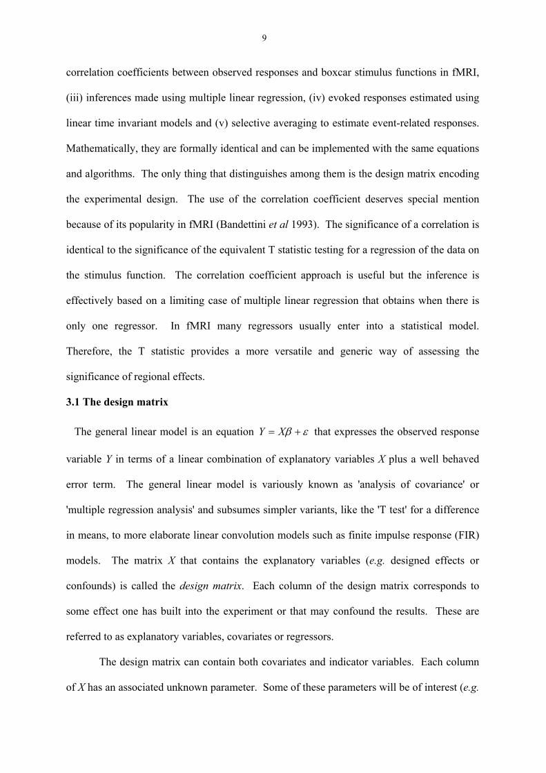
3.1 The design matrix The general linear model is an equation εβ += XY that expresses the observed response

variable Y in terms of a linear combination of explanatory variables X plus a well behaved

error term. The general linear model is variously known as 'analysis of covariance' or

'multiple regression analysis' and subsumes simpler variants, like the 'T test' for a difference

in means, to more elaborate linear convolution models such as finite impulse response (FIR)

models. The matrix X that contains the explanatory variables (e.g. designed effects or

confounds) is called the design matrix. Each column of the design matrix corresponds to

some effect one has built into the experiment or that may confound the results. These are

referred to as explanatory variables, covariates or regressors.

The design matrix can contain both covariates and indicator variables. Each column

of X has an associated unknown parameter. Some of these parameters will be of interest (e.g.

10

the effect of particular sensorimotor or cognitive condition or the regression coefficient of

hemodynamic responses on reaction time). The remaining parameters will be of no interest

and pertain to confounding effects (e.g. the effect of being a particular subject or the

regression slope of voxel activity on global activity).

The example in Figure 1 relates to a fMRI study of visual stimulation under four

conditions. The effects on the response variable are modeled in terms of functions of the

presence of these conditions (i.e. boxcars smoothed with a hemodynamic response function)

and constitute the first four columns of the design matrix. There then follows a series of

terms that are designed to remove or model low frequency variations in signal due to artifacts

such as aliased biorhythms and other drift terms. The final column is whole brain activity.

The relative contribution of each of these columns is assessed using standard least squares or

Bayesian estimation. Classical inferences about these contributions are made using T or F

statistics, depending upon whether one is looking at a particular linear combination (e.g. a

subtraction), or all of them together. Bayesian inferences are based on the posterior or

conditional probability that the contribution exceedeed some threshold, usually zero.

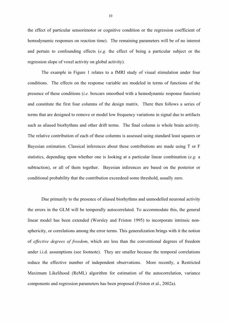
Due primarily to the presence of aliased biorhythms and unmodelled neuronal activity

the errors in the GLM will be temporally autocorrelated. To accommodate this, the general

linear model has been extended (Worsley and Friston 1995) to incorporate intrinsic non-

sphericity, or correlations among the error terms. This generalization brings with it the notion

of effective degrees of freedom, which are less than the conventional degrees of freedom

under i.i.d. assumptions (see footnote). They are smaller because the temporal correlations

reduce the effective number of independent observations. More recently, a Restricted

Maximum Likelihood (ReML) algorithm for estimation of the autocorrelation, variance

components and regression parameters has been proposed (Friston et al., 2002a).

11

3.2 Contrasts To assess effects of interest that are spanned by one or more columns in the design matrix

one uses a contrast (ie. a linear combination of parameter estimates). An example of a

contrast weight vector would be [-1 1 0 0..... ] to compare the difference in responses evoked

by two conditions, modeled by the first two condition-specific regressors in the design

matrix. Sometimes several contrasts of parameter estimates are jointly interesting. For

example, when using polynomial (Büchel et al 1996) or basis function expansions (see

section 3.1) of some experimental factor. In these instances, a matrix of contrast weights is

used that can be thought of as a collection of effects that one wants to test together. Such a

contrast may look like,

−……

00100001

which would test for the significance of the first or second parameter estimates. The fact that

the first weight is –1 as opposed to 1 has no effect on the test because F statistics are based

on sums of squares.

.

3.3 Temporal basis functions Functional MRI using Blood Oxygen Level Dependent (BOLD) contrast provides an index

of neuronal activity indirectly via changes in blood oxygenation levels. For a given impulse

of neuronal activity the fMRI signal peaks some 4-6 seconds later, then after 10 seconds or

so drops below zero and returns to baseline after 20 to 30 seconds. This response varies from

subject to subject and from voxel to voxel and this variation can be captured using temporal

basis functions.

12

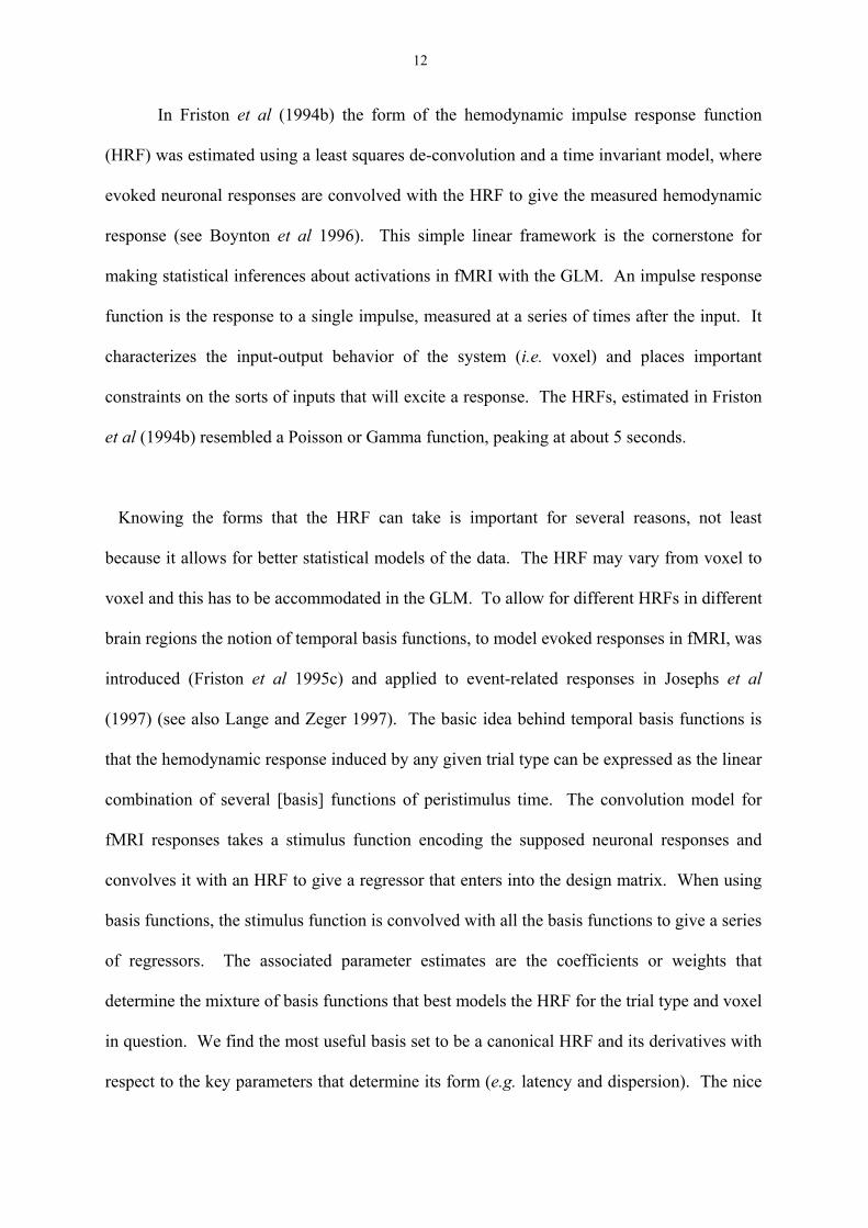
In Friston et al (1994b) the form of the hemodynamic impulse response function

(HRF) was estimated using a least squares de-convolution and a time invariant model, where

evoked neuronal responses are convolved with the HRF to give the measured hemodynamic

response (see Boynton et al 1996). This simple linear framework is the cornerstone for

making statistical inferences about activations in fMRI with the GLM. An impulse response

function is the response to a single impulse, measured at a series of times after the input. It

characterizes the input-output behavior of the system (i.e. voxel) and places important

constraints on the sorts of inputs that will excite a response. The HRFs, estimated in Friston

et al (1994b) resembled a Poisson or Gamma function, peaking at about 5 seconds.

Knowing the forms that the HRF can take is important for several reasons, not least

because it allows for better statistical models of the data. The HRF may vary from voxel to

voxel and this has to be accommodated in the GLM. To allow for different HRFs in different

brain regions the notion of temporal basis functions, to model evoked responses in fMRI, was

introduced (Friston et al 1995c) and applied to event-related responses in Josephs et al

(1997) (see also Lange and Zeger 1997). The basic idea behind temporal basis functions is

that the hemodynamic response induced by any given trial type can be expressed as the linear

combination of several [basis] functions of peristimulus time. The convolution model for

fMRI responses takes a stimulus function encoding the supposed neuronal responses and

convolves it with an HRF to give a regressor that enters into the design matrix. When using

basis functions, the stimulus function is convolved with all the basis functions to give a series

of regressors. The associated parameter estimates are the coefficients or weights that

determine the mixture of basis functions that best models the HRF for the trial type and voxel

in question. We find the most useful basis set to be a canonical HRF and its derivatives with

respect to the key parameters that determine its form (e.g. latency and dispersion). The nice

13

thing about this approach is that it can partition differences among evoked responses into

differences in magnitude, latency or dispersion, that can be tested for using specific contrasts

(Friston et al 1998b).

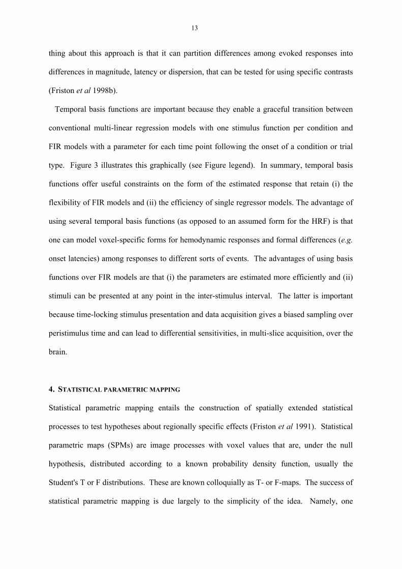
Temporal basis functions are important because they enable a graceful transition between

conventional multi-linear regression models with one stimulus function per condition and

FIR models with a parameter for each time point following the onset of a condition or trial

type. Figure 3 illustrates this graphically (see Figure legend). In summary, temporal basis

functions offer useful constraints on the form of the estimated response that retain (i) the

flexibility of FIR models and (ii) the efficiency of single regressor models. The advantage of

using several temporal basis functions (as opposed to an assumed form for the HRF) is that

one can model voxel-specific forms for hemodynamic responses and formal differences (e.g.

onset latencies) among responses to different sorts of events. The advantages of using basis

functions over FIR models are that (i) the parameters are estimated more efficiently and (ii)

stimuli can be presented at any point in the inter-stimulus interval. The latter is important

because time-locking stimulus presentation and data acquisition gives a biased sampling over

peristimulus time and can lead to differential sensitivities, in multi-slice acquisition, over the

brain.

4. STATISTICAL PARAMETRIC MAPPING

Statistical parametric mapping entails the construction of spatially extended statistical

processes to test hypotheses about regionally specific effects (Friston et al 1991). Statistical

parametric maps (SPMs) are image processes with voxel values that are, under the null

hypothesis, distributed according to a known probability density function, usually the

Student's T or F distributions. These are known colloquially as T- or F-maps. The success of

statistical parametric mapping is due largely to the simplicity of the idea. Namely, one

14

analyses each and every voxel using any standard (univariate) statistical test. The resulting

statistical parameters are assembled into an image - the SPM. SPMs are interpreted as

spatially extended statistical processes by referring to the probabilistic behavior of Gaussian

fields (Adler 1981, Worsley et al 1992, Friston et al 1994a, Worsley et al 1996). Gaussian

random fields model both the univariate probabilistic characteristics of a SPM and any non-

stationary spatial covariance structure. 'Unlikely' excursions of the SPM are interpreted as

regionally specific effects, attributable to the sensorimotor or cognitive process that has been

manipulated experimentally.

Over the years statistical parametric mapping has come to refer to the conjoint use of the

general linear model (GLM) and Gaussian random field (GRF) theory to analyze and make

classical inferences about spatially extended data through statistical parametric maps (SPMs).

The GLM is used to estimate some parameters that could explain the spatially continuous

data in exactly the same way as in conventional analysis of discrete data. GRF theory is used

to resolve the multiple comparison problem that ensues when making inferences over a

volume of the brain. GRF theory provides a method for correcting p values for the search

volume of an SPM and plays the same role for continuous data (i.e. images) as the

Bonferonni correction for the number of discontinuous or discrete statistical tests. The

approach was called SPM for three reasons; (i) To acknowledge Significance Probability

Mapping, the use of interpolated pseudo-maps of p values used to summarize the analysis of

multi-channel ERP studies. (ii) For consistency with the nomenclature of parametric maps of

physiological or physical parameters (e.g. regional cerebral blood flow rCBF or volume

rCBV parametric maps). (iii) In reference to the parametric statistics that comprise the maps.

Despite its simplicity there are some fairly subtle motivations for the approach that deserve

mention. Usually, given a response or dependent variable comprising many thousands of

voxels one would use multivariate analyses as opposed to the mass-univariate approach that

15

SPM represents. The problems with multivariate approaches are that; (i) they do not support

inferences about regionally specific effects, (ii) they require more observations than the

dimension of the response variable (i.e. number of voxels) and (iii), even in the context of

dimension reduction, they are less sensitive to focal effects than mass-univariate approaches.

A heuristic argument, for their relative lack of power, is that multivariate approaches (in their

most general form) estimate the model’s error covariances using lots of parameters (e.g. the

covariance between the errors at all pairs of voxels). In general, the more parameters an

estimation procedure has to deal with, the more variable the estimate of any one parameter

becomes. This renders any single estimate less efficient.

Multivariate approaches consider voxels as different levels of an experimental or treatment

factor and use classical analysis of variance, not at each voxel (c.f. SPM), but by considering

the data sequences from all voxels together, as replications over voxels. The problem here is

that regional changes in error variance, and spatial correlations in the data, induce profound

non-sphericity1 in the error terms. This non-sphericity would require large numbers of

parameters to be estimated for each voxel using conventional techniques. In SPM the non-

sphericity is parameterized in a very parsimonious way with just two parameters for each

voxel. These are the error variance and smoothness estimators. This minimal

parameterization lends SPM a sensitivity that surpasses multivariate approaches. SPM can

do this because GRF theory implicitly imposes constraints on the non-sphericity implied by

the continuous and [spatially] extended nature of the data. This is something that

conventional multivariate and equivalent univariate approaches do not accommodate, to their

cost.

1 Sphericity refers to the assumption of identically and independently distributed error terms (i.i.d.). Under i.i.d. the probability density function of the errors, from all observations, has spherical iso-contours, hence sphericity. Deviations from either of the i.i.d. criteria constitute non-sphericity. If the error terms are not identically distributed then different observations have different error variances. Correlations among error terms reflect dependencies among the error terms (e.g. serial correlation in fMRI time series) and constitute the second component of non-sphericity. In fMRI both spatial and temporal non-sphericity can be quite profound issues.

16

Some analyses use statistical maps based on non-parametric tests that eschew distributional

assumptions about the data eg. non-parametric approaches (Nichols and Holmes, 2001).

These approaches are generally less powerful (i.e. less sensitive) than parametric approaches

(see Aguirre et al 1998). However, they have an important role in evaluating the

assumptions behind parametric approaches and may supercede in terms of sensitivity when

these assumptions are violated (e.g. when degrees of freedom are very small and voxel sizes

are large in relation to smoothness).

4.1 Random Field Theory

Classical inferences using SPMs can be of two sorts depending on whether one knows where

to look in advance. With an anatomically constrained hypothesis, about effects in a

particular brain region, the uncorrected p value associated with the height or extent of that

region in the SPM can be used to test the hypothesis. With an anatomically open hypothesis

(i.e. a null hypothesis that there is no effect anywhere in a specified volume of the brain) a

correction for multiple dependent comparisons is necessary. The theory of random fields

provides a way of adjusting the p-value that takes into account the fact that neighboring

voxels are not independent by virtue of continuity in the original data. Provided the data are

sufficiently smooth the GRF correction is less severe (i.e. is more sensitive) than a

Bonferroni correction for the number of voxels. As noted above GRF theory deals with the

multiple comparisons problem in the context of continuous, spatially extended statistical

fields, in a way that is analogous to the Bonferroni procedure for families of discrete

statistical tests. There are many ways to appreciate the difference between GRF and

Bonferroni corrections. Perhaps the most intuitive is to consider the fundamental difference

between an SPM and a collection of discrete T values. When declaring a connected volume

or region of the SPM to be significant, we refer collectively to all the voxels that comprise

17

that volume. The false positive rate is expressed in terms of connected [excursion] sets of

voxels above some threshold, under the null hypothesis of no activation. This is not the

expected number of false positive voxels. One false positive region may contain hundreds of

voxels, if the SPM is very smooth. A Bonferroni correction would control the expected

number of false positive voxels, whereas GRF theory controls the expected number of false

positive regions. Because a false positive region can contain many voxels the corrected

threshold under a GRF correction is much lower, rendering it much more sensitive. In fact

the number of voxels in a region is somewhat irrelevant because the correction is a function

of smoothness. The GRF correction discounts voxel size by expressing the search volume in

terms of smoothness or resolution elements (Resels). This intuitive perspective is expressed

formally in terms of differential topology using the Euler characteristic (Worsley et al 1992).

At high thresholds the Euler characteristic corresponds to the number of regions exceeding

the threshold.

There are only two assumptions underlying the use of the GRF correction: (i) The error

fields (but not necessarily the data) are a reasonable lattice approximation to an underlying

random field with a multivariate Gaussian distribution. (ii) These fields are continuous, with

a differentiable and invertible autocorrelation function. A common misconception is that the

autocorrelation function has to be Gaussian. It does not. The only way in which these

assumptions can be violated is if; (i) the data are not smoothed (with or without sub-sampling

to preserve resolution), violating the reasonable lattice assumption or (ii) the statistical model

is mis-specified so that the errors are not normally distributed. Early formulations of the GRF

correction were based on the assumption that the spatial correlation structure was wide-sense

stationary. This assumption can now be relaxed due to a revision of the way in which the

smoothness estimator enters the correction procedure (Kiebel et al 1999). In other words, the

corrections retain their validity, even if the smoothness varies from voxel to voxel.

18

5. POSTERIOR PROBABILITY MAPPING

Despite its success, statistical parametric mapping has a number of fundamental limitations.

In SPM the p value, ascribed to a particular effect, does not reflect the likelihood that the

effect is present but simply the probability of getting the observed data in the effect's

absence. If sufficiently small, this p value can be used to reject the null hypothesis that the

effect is negligible. There are several shortcomings of this classical approach. Firstly, one

can never reject the alternate hypothesis (i.e. say that an activation has not occurred) because

the probability that an effect is exactly zero is itself zero. This is problematic, for example,

in trying to establish double dissociations or indeed functional segregation; one can never say

one area responds to colour but not motion and another responds to motion but not colour.

Secondly, because the probability of an effect being zero is vanishingly small, given enough

scans or subjects one can always demonstrate a significant effect at every voxel. This fallacy

of classical inference is becoming relevant practically, with the thousands of scans entering

into some fixed-effect analyses of fMRI data. The issue here is that a trivially small

activation can be declared significant if there are sufficient degrees of freedom to render the

variability of the activation's estimate small enough. A third problem, that is specific to

SPM, is the correction or adjustment applied to the p values to resolve the multiple

comparison problem. This has the somewhat nonsensical effect of changing the inference

about one part of the brain in a way that is contingent on whether another part is examined.

Put simply, the threshold increases with search volume, rendering inference very sensitive to

what that inference encompasses. Clearly the probability that any voxel has activated does

not change with the search volume and yet the classical p value does.

19

All these problems would be eschewed by using the probability that a voxel had activated,

or indeed its activation was greater than some threshold. This sort of inference is precluded

by classical approaches, which simply give the likelihood of getting the data, given no

activation. What one would really like is the probability distribution of the activation given

the data. This is the posterior probability used in Bayesian inference. The posterior

distribution requires both the likelihood, afforded by assumptions about the distribution of

errors, and the prior probability of activation. These priors can enter as known values or can

be estimated from the data, provided we have observed multiple instances of the effect we

are interested in. The latter is referred to as empirical Bayes. A key point here is that we do

assess repeatedly the same effect over different voxels, and we are therefore in a position to

adopt an empirical Bayesian approach (Friston and Penny, 2003).

5.1 Empirical Example

In this section we compare and contrast Bayesian and classical inference using PPMs and

SPMs based on real data. The data set comprised data from a study of attention to visual

motion (Büchel & Friston 1997). The data used here came from the first subject studied.

This subject was scanned at 2T to give a time series of 360 images comprising 10 block

epochs of different visual motion conditions. These conditions included a fixation condition,

visual presentation of static dots, visual presentation of radially moving dots under attention

and no-attention conditions. In the attention condition subjects were asked to attend to

changes in speed (which did not actually occur). This attentional manipulation was validated

post-hoc using psychophysics and the motion after-effect. Further details of the data

acquisition are given in the caption to Figure 8. These data were analysed using a

conventional SPM procedure and the empirical Bayesian approach described in the previous

section. The ensuing SPMs and PPMs are presented in Figures 4 and 5. We used a contrast

20

that tested for the effect of visual motion above and beyond that due to photic stimulation

with stationary dots.

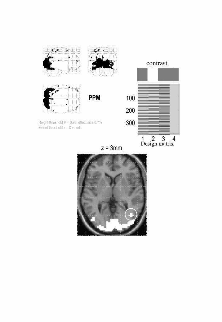
The difference between the PPM and SPM is immediately apparent on inspection of Figures

4 and 5. Here the threshold for the PPM was 0.7% (equivalent to percentage whole brain

mean signal). Only voxels that exceed 95% confidence are shown. These are restricted to

visual and extrastriate cortex involved in motion processing. The critical thing to note is that

the corresponding SPM identifies a smaller number of voxels than the PPM. Indeed the SPM

appears to have missed a critical and bilaterally represented part of the V5 complex (circled

cluster on the PPM in the lower panel of Figure 4). The SPM is more conservative because

the correction for multiple comparisons in these data is very severe, rendering classical

inference relatively insensitive. It is interesting to note that dynamic motion in the visual

field has such widespread (if small) effects at a hemodynamic level.

6. DYNAMIC CAUSAL MODELLING

Dynamic Causal Modelling (DCM) (Friston et al., 2003) is used to make inferences about

functional integration from fMRI time series. The term 'causal' in DCM arises because the

brain is treated as a deterministic dynamical system in which external inputs cause changes in

neuronal activity which in turn cause changes in the resulting BOLD (Blood Oxygen Level

Dependent) signal that is measured with fMRI. This is to be contrasted with a conventional

GLM where there is no explicit representation of neuronal activity. The second main

difference to the GLM is that DCM allows for interactions between regions. Of course, it is

this interaction which is central to the study of functional integration.

21

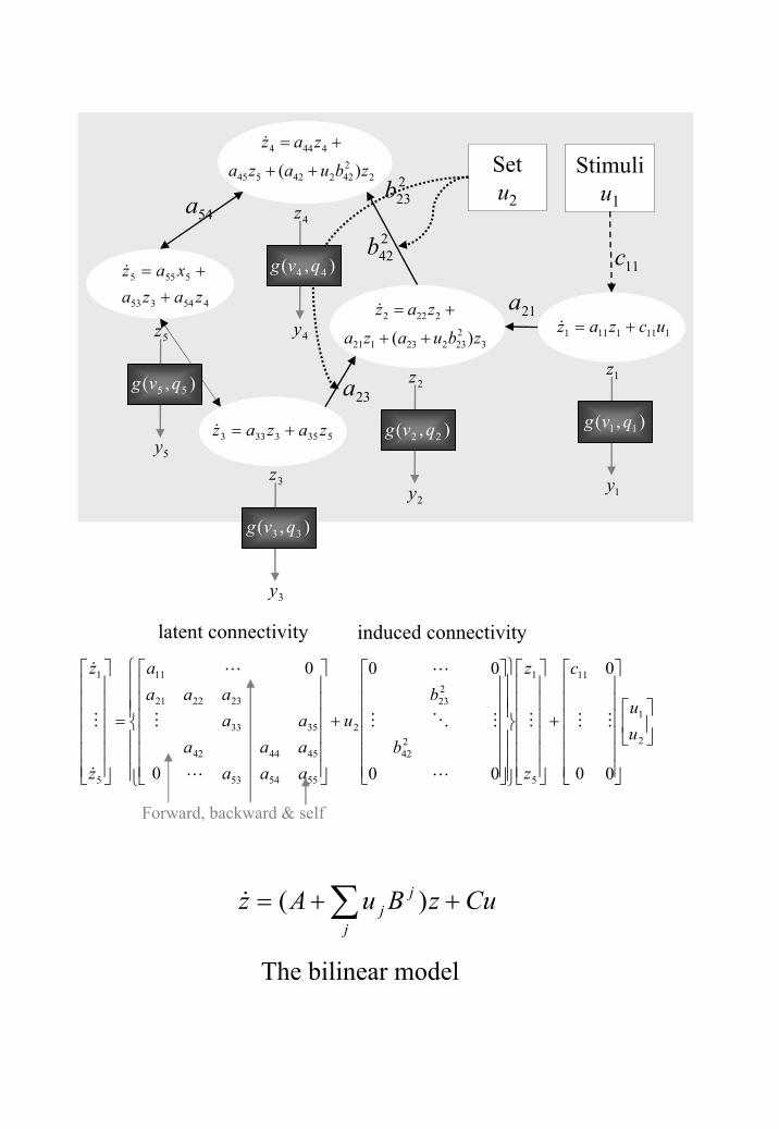
Current DCMs for fMRI comprise a bilinear model for the neurodynamics and an extended

Balloon model for the hemodynamics. These are shown in Figures 6 and 7. The

neurodynamics are described by the multivariate differential equation shown in Figure 6.

This is known as a bilinear model because the dependent variable, z , is linearly dependent

on the product of z and u . That u and z combine in a multiplicative fashion endows the

model with `nonlinear' dynamics that can be understood as a nonstationary linear system that

changes according to experimental manipulation u . Importantly, because u is known,

parameter estimation is relatively simple.

Connectivity in DCM is characterised by a set of `intrinsic connections', A , that

specify which regions are connected and whether these connections are unidirectional or

bidirectional. We also define a set of input connections, C , that specify which inputs are

connected to which regions, and a set of modulatory or bilinear connections, jB , that specify

which intrinsic connections can be changed by which inputs. The overall specification of

input, intrinsic and modulatory connectivity comprise our assumptions about model structure.

This in turn represents a scientific hypothesis about the structure of the large-scale neuronal

network mediating the underlying sensorimotor or cognitive function.

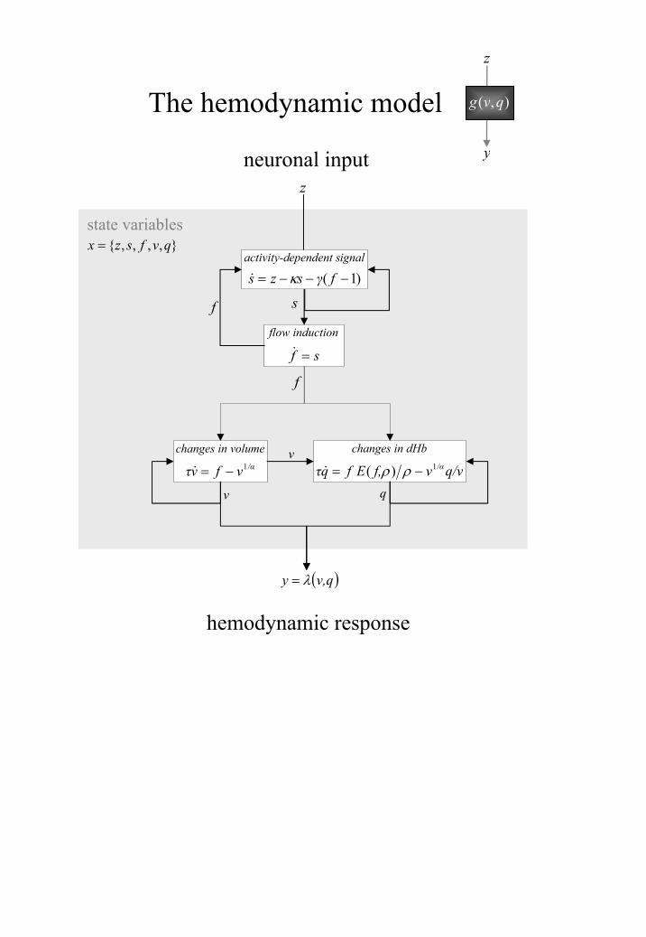
In DCM, neuronal activity gives rise to hemodynamic activity by a dynamic process

described by an extended Balloon model. This involves a set of hemodynamic state variables,

state equations and hemodynamic parameters shown in Figure 7. Together these equations

describe a nonlinear hemodynamic process that may be regarded as a biophysically informed

generalisation of the linear convolution models used in the GLM. It is possible to describe

the second-order behaviour of this process (ie. how the response to one stimulus is changed

by a preceding stimulus) using Volterra kernels.

22

6.1 Empirical example

We now return to the attention to visual motion study described in section 5.1 so as to make

inferences about functional integration. Figure 8b shows the location of the regions that

entered the DCM (Figure 8b - insert). These regions were based on maxima from

conventional SPMs testing for the effects of photic stimulation, motion and attention.

Regional time courses were taken as the first eigenvariate of spherical volumes of interest

centred on the maxima shown in Figure 8. The inputs, in this example, comprise one sensory

perturbation and two contextual inputs. The sensory input was simply the presence of photic

stimulation and the first contextual one was presence of motion in the visual field. The

second contextual input, encoding attentional set, was unity during attention to speed changes

and zero otherwise. The outputs corresponded to the four regional eigenvariates in (Figure

8b). The intrinsic connections were constrained to conform to a hierarchical pattern in which

each area was reciprocally connected to its supraordinate area. Photic stimulation entered at,

and only at, V1. The effect of motion in the visual field was modelled as a bilinear

modulation of the V1 to V5 connectivity and attention was allowed to modulate the

backward connections from IFG and SPC.

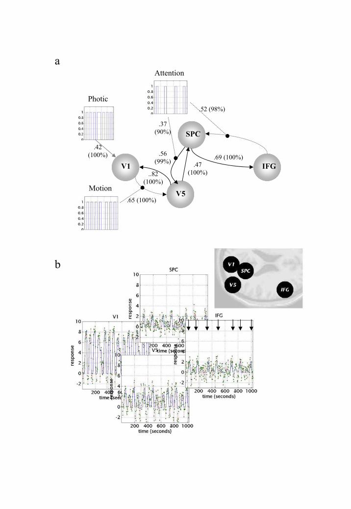
The results of the DCM are shown in Figure 8a. Of primary interest here is the

modulatory effect of attention that is expressed in terms of the bilinear coupling parameters

for this third input. As hoped, we can be highly confident that attention modulates the

backward connections from IFG to SPC and from SPC to V5. Indeed, the influences of IFG

on SPC are negligible in the absence of attention (dotted connection in Figure 8a). It is

important to note that the only way that attentional manipulation could affect brain responses

was through this bilinear effect. Attention-related responses are seen throughout the system

(attention epochs are marked with arrows in the plot of IFG responses in Figure 8b). This

23

attentional modulation is accounted for, sufficiently, by changing just two connections. This

change is, presumably, instantiated by instructional set at the beginning of each epoch. The

second thing, this analysis illustrates, is the how functional segregation is modelled in DCM.

Here one can regard V1 as a ‘segregating’ motion from other visual information and

distributing it to the motion-sensitive area V5. This segregation is modelled as a bilinear

‘enabling’ of V1 to V5 connections when, and only when, motion is present. Note that in the

absence of motion the intrinsic V1 to V5 connection was trivially small (in fact the MAP

estimate was -0.04). The key advantage of entering motion through a bilinear effect, as

opposed to a direct effect on V5, is that we can finesse the inference that V5 shows motion-

selective responses with the assertion that these responses are mediated by afferents from V1.

The two bilinear effects above represent two important aspects of functional integration that

DCM was designed to characterise.

CONCLUSION

Due to the concise nature of this review we have been unable to cover a number of

related topics. These include computational neuroanatomy, analysis of group data (whether

structural or functional) using either fixed or random-effect analysis. In the context of the

GLM we omitted discussion of event-related versus block designs, parametric and factorial

designs and the factors underlying an efficient experimental design. We refer interested

readers to the recent volume entitled ‘Human Brain Function’ (Frackowiak et al. 2003) that

builds upon the basic issues introduced here. These methods and all of the procedures

covered in this review have been implemented in a public-domain software package called

SPM2 available from http://www.fil.ion.ucl.ac.uk/spm/.

24

References

Adler RJ. (1981) In “The geometry of random fields”. Wiley New York

Aguirre GK Zarahn E and D'Esposito M. (1998) A critique of the use of the Kolmogorov-

Smirnov (KS) statistic for the analysis of BOLD fMRI data. Mag. Res. Med. 39:500-505

Andersson JL, Hutton C, Ashburner J, Turner R, Friston K. (2001) Modeling geometric

deformations in EPI time series. NeuroImage. 13:903-19

Ashburner J Neelin P Collins DL Evans A and Friston K. (1997) Incorporating prior

knowledge into image registration. NeuroImage 6:344-352

Bandettini PA Jesmanowicz A Wong EC and Hyde JS. (1993) Processing strategies for time

course data sets in functional MRI of the human brain. Mag. Res. Med. 30:161-173

Boynton GM Engel SA Glover GH and Heeger DJ. (1996) Linear systems analysis of

functional magnetic resonance imaging in human V1. J Neurosci. 16:4207-4221

Büchel C Wise RJS Mummery CJ Poline J-B and Friston KJ. (1996) Nonlinear regression in

parametric activation studies. NeuroImage 4:60-66

Büchel C and Friston KJ. (1997) Modulation of connectivity in visual pathways by attention:

Cortical interactions evaluated with structural equation modeling and fMRI. Cerebral Cortex

7:768-778

Buchel C., Coull J. and Friston K.J. (1999) The predictive value of changes in effective

connectivity for human learning. Science, 283(5407), pp. 1538-41.

Frackowiak R., Friston K.J., Frith C., Dolan R., Price C., Zeki, S., Ashburner J. and Penny,

W. (2003) Human Brain Function, Elsevier Academic Press, 2nd Edition.

Friston KJ Frith CD Liddle PF and Frackowiak RSJ. (1991) Comparing functional (PET)

images: the assessment of significant change. J. Cereb. Blood Flow Metab. 11:690-699

25

Friston KJ Worsley KJ Frackowiak RSJ Mazziotta JC and Evans AC. (1994a) Assessing the

significance of focal activations using their spatial extent. Hum. Brain Mapp. 1:214-220

Friston KJ Jezzard PJ and Turner R. (1994b) Analysis of functional MRI time-series Hum.

Brain Mapp. 1:153-171

Friston KJ Ashburner J Frith CD Poline J-B Heather JD and Frackowiak RSJ. (1995a)

Spatial registration and normalization of images. Hum. Brain Mapp. 2:165-189

Friston KJ Frith CD Turner R and Frackowiak RSJ. (1995c) Characterizing evoked

hemodynamics with fMRI. NeuroImage 2:157-165

Friston KJ Williams S Howard R Frackowiak RSJ and Turner R. (1996a) Movement related

effects in fMRI time series. Mag. Res. Med. 35:346-355

Friston KJ Fletcher P Josephs O Holmes A Rugg MD and Turner R. (1998b) Event-related

fMRI: Characterizing differential responses. NeuroImage 7:30-40

Friston KJ, Penny W, Phillips C, Kiebel S, Hinton G and Ashburner J. (2002a) Classical and

Bayesian inference in neuroimaging: Theory. NeuroImage. 16:465-483

Friston KJ and Penny W (2003) Posterior probability maps and SPMs. NeuroImage.

19(3):1240-1249.

Friston KJ, Harrison L and Penny W (2003) Dynamic Causal Modelling. NeuroImage.

19(4):1273-1302.

Grootoonk S, Hutton C, Ashburner J, Howseman AM, Josephs O, Rees G, Friston KJ, Turner

R. (2000) Characterization and correction of interpolation effects in the realignment of fMRI

time series. NeuroImage. 11:49-57.

26

Jezzard P and Balaban RS. (1995) Correction for geometric distortion in echo-planar

images from B0 field variations. Mag. Res. Med. 34:65-73

Josephs O Turner R and Friston KJ. (1997) Event-related fMRI Hum. Brain Mapp. 5:243-

248

Kiebel SJ, Poline JB, Friston KJ, Holmes AP, Worsley KJ. (1999) Robust smoothness

estimation in statistical parametric maps using standardized residuals from the general linear

model. NeuroImage. 10:756-66.

Lange N and Zeger SL. (1997) Non-linear Fourier time series analysis for human brain

mapping by functional magnetic resonance imaging (with discussion) J Roy. Stat. Soc. Ser

C. 46:1-29

Nichols TE and Holmes AP. (2001) Nonparametric permutation tests for functional

neuroimaging: a primer with examples. Human Brain Mapping, 15, 1-25.

Talairach P and Tournoux J. (1988) “A Stereotactic coplanar atlas of the human brain“

Stuttgart Thieme.

Ungerleider, L. G. and Mishkin, M. (1982) in Analysis of Visual Behavior, eds. Ingle, D. J.,

Goodale, M. A. & Mansfield, R. J. W. (MIT Press, Cambridge, MA), pp. 549-586.

Worsley KJ Evans AC Marrett S and Neelin P. (1992) A three-dimensional statistical

analysis for rCBF activation studies in human brain. J Cereb. Blood Flow Metab. 12:900-

918

Worsley KJ and Friston KJ. (1995) Analysis of fMRI time-series revisited - again.

NeuroImage 2:173-181

Worsley KJ Marrett S Neelin P Vandal AC Friston KJ and Evans AC. (1996) A unified

statistical approach or determining significant signals in images of cerebral activation. Hum.

Brain Mapp. 4:58-73

27

Zeki S, Watson JD, Lueck CJ, Friston KJ, Kennard C and RS Frackowiak (1991) A direct

demonstration of functional specialization in human visual cortex. Journal of Neuroscience,

Vol 11, pp. 641-649.

Figure Legends

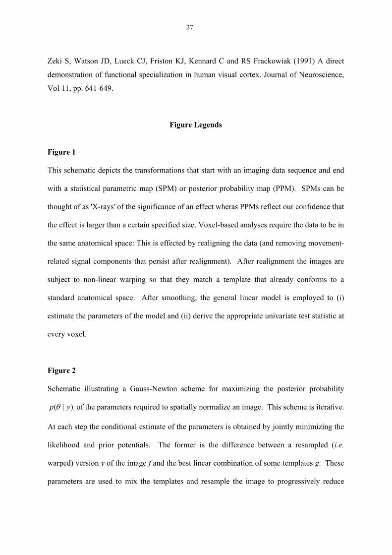
Figure 1

This schematic depicts the transformations that start with an imaging data sequence and end

with a statistical parametric map (SPM) or posterior probability map (PPM). SPMs can be

thought of as 'X-rays' of the significance of an effect wheras PPMs reflect our confidence that

the effect is larger than a certain specified size. Voxel-based analyses require the data to be in

the same anatomical space: This is effected by realigning the data (and removing movement-

related signal components that persist after realignment). After realignment the images are

subject to non-linear warping so that they match a template that already conforms to a

standard anatomical space. After smoothing, the general linear model is employed to (i)

estimate the parameters of the model and (ii) derive the appropriate univariate test statistic at

every voxel.

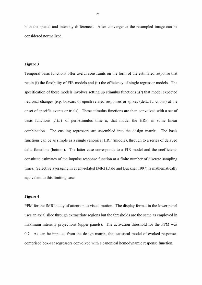
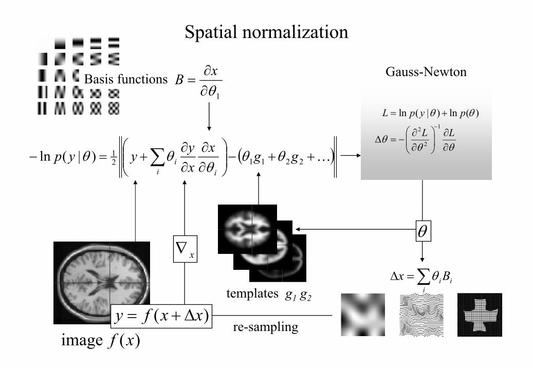
Figure 2

Schematic illustrating a Gauss-Newton scheme for maximizing the posterior probability

)|( yp θ of the parameters required to spatially normalize an image. This scheme is iterative.

At each step the conditional estimate of the parameters is obtained by jointly minimizing the

likelihood and prior potentials. The former is the difference between a resampled (i.e.

warped) version y of the image f and the best linear combination of some templates g. These

parameters are used to mix the templates and resample the image to progressively reduce

28

both the spatial and intensity differences. After convergence the resampled image can be

considered normalized.

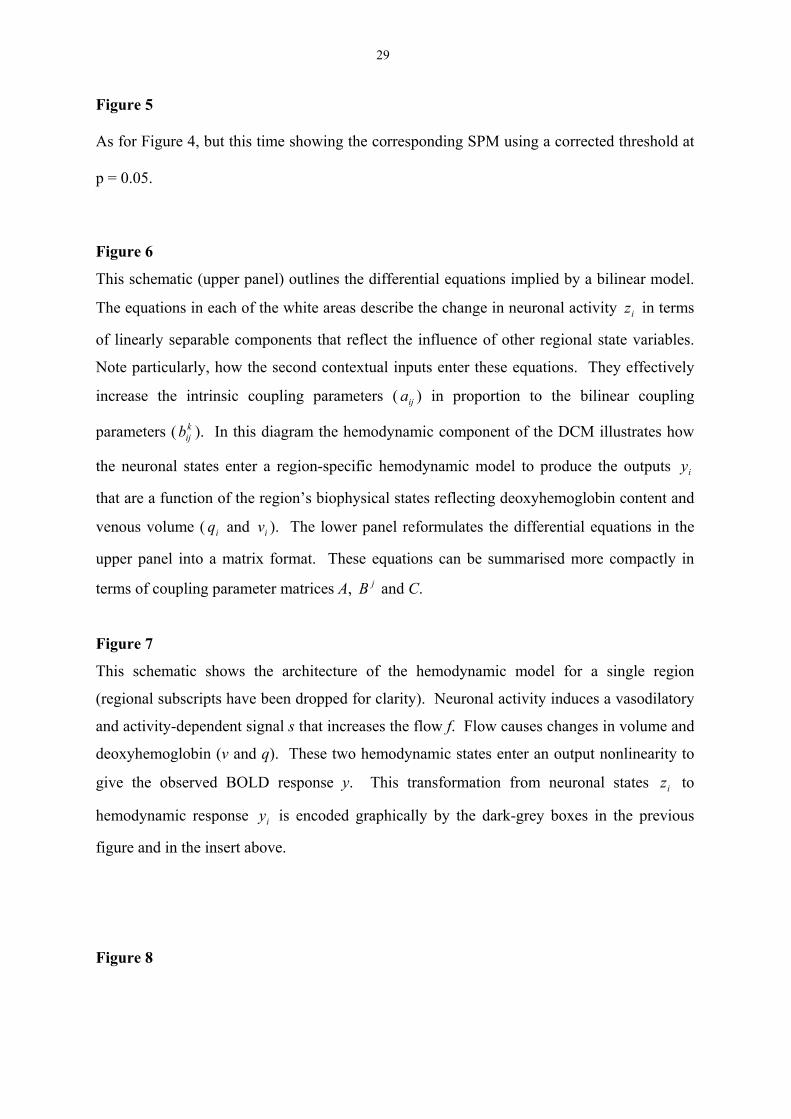
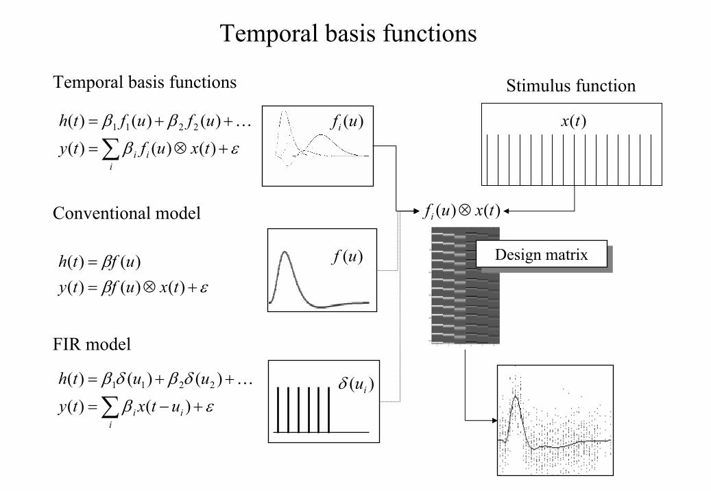
Figure 3

Temporal basis functions offer useful constraints on the form of the estimated response that

retain (i) the flexibility of FIR models and (ii) the efficiency of single regressor models. The

specification of these models involves setting up stimulus functions x(t) that model expected

neuronal changes [e.g. boxcars of epoch-related responses or spikes (delta functions) at the

onset of specific events or trials]. These stimulus functions are then convolved with a set of

basis functions )(ufi of peri-stimulus time u, that model the HRF, in some linear

combination. The ensuing regressors are assembled into the design matrix. The basis

functions can be as simple as a single canonical HRF (middle), through to a series of delayed

delta functions (bottom). The latter case corresponds to a FIR model and the coefficients

constitute estimates of the impulse response function at a finite number of discrete sampling

times. Selective averaging in event-related fMRI (Dale and Buckner 1997) is mathematically

equivalent to this limiting case.

Figure 4

PPM for the fMRI study of attention to visual motion. The display format in the lower panel

uses an axial slice through extrastriate regions but the thresholds are the same as employed in

maximum intensity projections (upper panels). The activation threshold for the PPM was

0.7. As can be imputed from the design matrix, the statistical model of evoked responses

comprised box-car regressors convolved with a canonical hemodynamic response function.

29

Figure 5

As for Figure 4, but this time showing the corresponding SPM using a corrected threshold at

p = 0.05.

Figure 6

This schematic (upper panel) outlines the differential equations implied by a bilinear model.

The equations in each of the white areas describe the change in neuronal activity iz in terms

of linearly separable components that reflect the influence of other regional state variables.

Note particularly, how the second contextual inputs enter these equations. They effectively

increase the intrinsic coupling parameters ( ija ) in proportion to the bilinear coupling

parameters ( kijb ). In this diagram the hemodynamic component of the DCM illustrates how

the neuronal states enter a region-specific hemodynamic model to produce the outputs iy

that are a function of the region’s biophysical states reflecting deoxyhemoglobin content and

venous volume ( iq and iv ). The lower panel reformulates the differential equations in the

upper panel into a matrix format. These equations can be summarised more compactly in

terms of coupling parameter matrices A, jB and C.

Figure 7

This schematic shows the architecture of the hemodynamic model for a single region

(regional subscripts have been dropped for clarity). Neuronal activity induces a vasodilatory

and activity-dependent signal s that increases the flow f. Flow causes changes in volume and

deoxyhemoglobin (v and q). These two hemodynamic states enter an output nonlinearity to

give the observed BOLD response y. This transformation from neuronal states iz to

hemodynamic response iy is encoded graphically by the dark-grey boxes in the previous

figure and in the insert above.

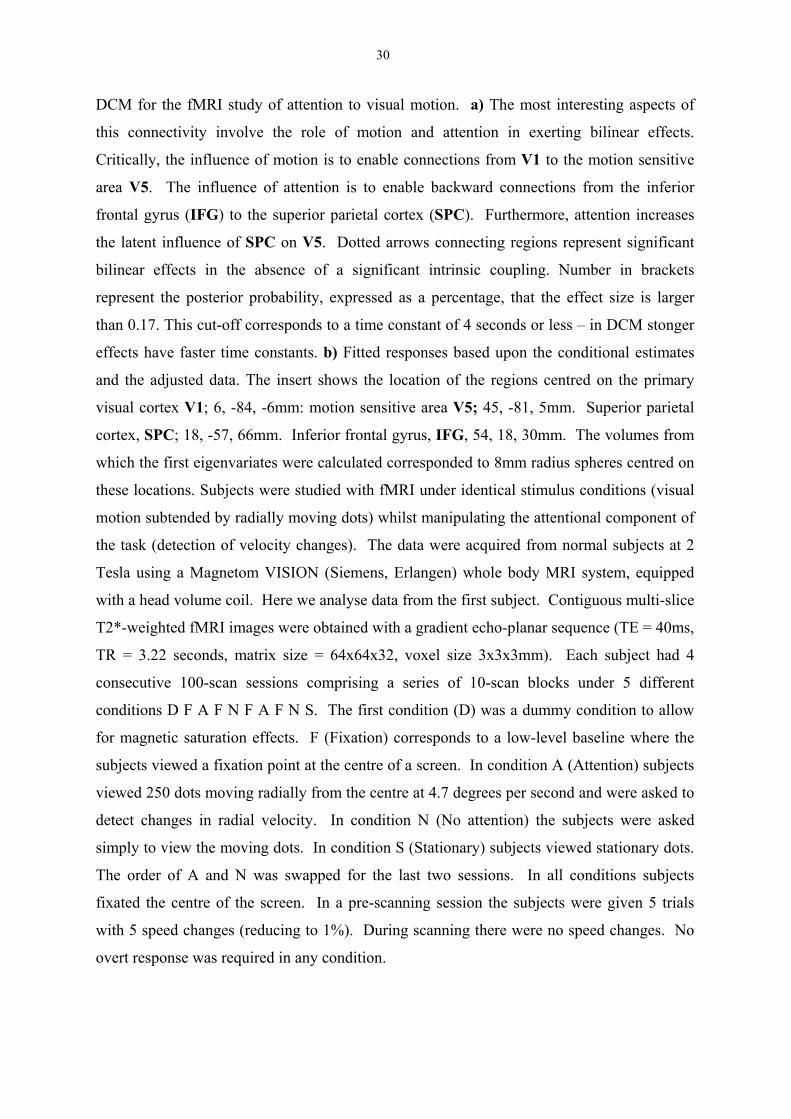
Figure 8

30

DCM for the fMRI study of attention to visual motion. a) The most interesting aspects of

this connectivity involve the role of motion and attention in exerting bilinear effects.

Critically, the influence of motion is to enable connections from V1 to the motion sensitive

area V5. The influence of attention is to enable backward connections from the inferior

frontal gyrus (IFG) to the superior parietal cortex (SPC). Furthermore, attention increases

the latent influence of SPC on V5. Dotted arrows connecting regions represent significant

bilinear effects in the absence of a significant intrinsic coupling. Number in brackets

represent the posterior probability, expressed as a percentage, that the effect size is larger

than 0.17. This cut-off corresponds to a time constant of 4 seconds or less – in DCM stonger

effects have faster time constants. b) Fitted responses based upon the conditional estimates

and the adjusted data. The insert shows the location of the regions centred on the primary

visual cortex V1; 6, -84, -6mm: motion sensitive area V5; 45, -81, 5mm. Superior parietal

cortex, SPC; 18, -57, 66mm. Inferior frontal gyrus, IFG, 54, 18, 30mm. The volumes from

which the first eigenvariates were calculated corresponded to 8mm radius spheres centred on

these locations. Subjects were studied with fMRI under identical stimulus conditions (visual

motion subtended by radially moving dots) whilst manipulating the attentional component of

the task (detection of velocity changes). The data were acquired from normal subjects at 2

Tesla using a Magnetom VISION (Siemens, Erlangen) whole body MRI system, equipped

with a head volume coil. Here we analyse data from the first subject. Contiguous multi-slice

T2*-weighted fMRI images were obtained with a gradient echo-planar sequence (TE = 40ms,

TR = 3.22 seconds, matrix size = 64x64x32, voxel size 3x3x3mm). Each subject had 4

consecutive 100-scan sessions comprising a series of 10-scan blocks under 5 different

conditions D F A F N F A F N S. The first condition (D) was a dummy condition to allow

for magnetic saturation effects. F (Fixation) corresponds to a low-level baseline where the

subjects viewed a fixation point at the centre of a screen. In condition A (Attention) subjects

viewed 250 dots moving radially from the centre at 4.7 degrees per second and were asked to

detect changes in radial velocity. In condition N (No attention) the subjects were asked

simply to view the moving dots. In condition S (Stationary) subjects viewed stationary dots.

The order of A and N was swapped for the last two sessions. In all conditions subjects

fixated the centre of the screen. In a pre-scanning session the subjects were given 5 trials

with 5 speed changes (reducing to 1%). During scanning there were no speed changes. No

overt response was required in any condition.

Data analysis stream

Statistical parametric map (SPM)or

Posterior probability map (PPM)

Image time-series

Parameter estimates

Design matrix

Template

Kernel

Normalisation

Realignment Smoothing General linear model

re-sampling

∑=∆i

iiBx θ

( )…++−

∂∂

∂∂

+=− ∑ 221121)|(ln ggx

xyyyp

i ii θθ

θθθ

Basis functions1θ∂

∂=

xB

)( xxfy ∆+=templates g1 g2

12

2

ln ( | ) ln ( )L p y p

L L

θ θ

θθ θ

−

= +

∂ ∂∆ = − ∂ ∂

Gauss-Newton

θ

Spatial normalization

x∇

)( image xf

Temporal basis functions

Conventional model

FIR model

Temporal basis functions

εβδβδβ+−=

++=

∑i

ii utxtyuuth

)()()()()( 2211 …

εββ

+⊗==

)()()()()(

txuftyufth

εβββ

+⊗=

++=

∑i

ii txuftyufufth)()()()()()( 2211 …

Stimulus function

)(ufi

)(uf

)( iuδ

)()( txufi ⊗

Design matrixDesign matrix

)(tx

PPM

Height threshold P = 0.95, effect size 0.7%Extent threshold k = 0 voxels

Design matrix1 2 3 4

100

200

300

contrast

z = 3mm

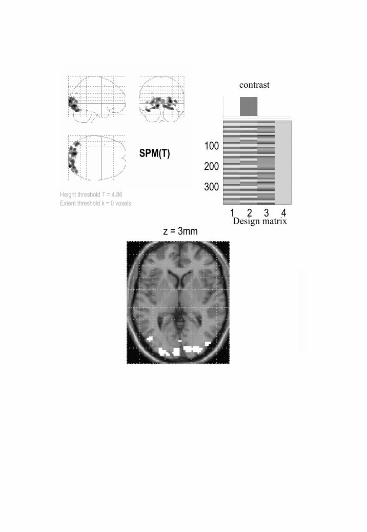
SPM(T)

Height threshold T = 4.86Extent threshold k = 0 voxels

Design matrix1 2 3 4

100

200

300

contrast

z = 3mm

Setu2

Stimuliu1

1111111 uczaz +=

5353333 zazaz +=

454353

5555

zazaxaz

++= 11c

21a

223b

23a

54a242b

),( 11 qvg

1z

1y

),( 22 qvg

2z

2y

),( 33 qvg

3z

3y

),( 44 qvg

4z

4y

),( 55 qvg

5z

5y

latent connectivity induced connectivity

Forward, backward & self

+

+

=

2

1

11

5

1

242

223

2

555453

454442

3533

232221

11

5

1

00

0

00

00

0

0

uu

c

z

z

b

bu

aaaaaaaa

aaaa

z

z

CuzBuAzj

jj ++= ∑ )(

The bilinear model

2242242545

4444

)( zbuazazaz++

+=

3223223121

2222

)( zbuazazaz++

+=

sftionflow induc

=

( )v,q y λ=

z

s

v

f

state variables

neuronal input

hemodynamic response

vq

The hemodynamic model

},,,,{ qvfszx =

q/vvf,Efqτ /α

dHbchanges in1)( −= ρρ/αvfvτ

volumechanges in1−=

f

q

),( qvg

z

y

)1( −−−= fγszsignalependent sactivity-d

κ

a

b

V1 IFG

V5

SPC

Motion

Photic

Attention

..82(100%)

.42(100%)

.37(90%)

.69 (100%).47

(100%)

.65 (100%)

.52 (98%)

.56(99%)