Bayesian Inference

SPM EEG-MEG Course

“The true logic for this world is the calculus of Probabilities, which takes account of the magnitude of the probability which is, or ought to be, in a reasonable man's mind.” James Clerk Maxwell (1850)

Jérémie Mattout Lyon Neuroscience Research Center, France

With many thanks to Jean Daunizeau

Guillaume Flandin Karl Friston Will Penny

- General principles - The Bayesian way - SPM examples

Outline

- General principles - The Bayesian way - SPM examples

Statistics: concerned with the collection, analysis and interpretation of data to make decisions

Applied statistics

Theoretical statistics Descriptive statistics summary statistics, graphics…

Inferential statistics Data interpretations, decision making (Modeling, accounting for randomness and unvertainty, hypothesis testing, infering hidden parameters)

A starting point

Probability

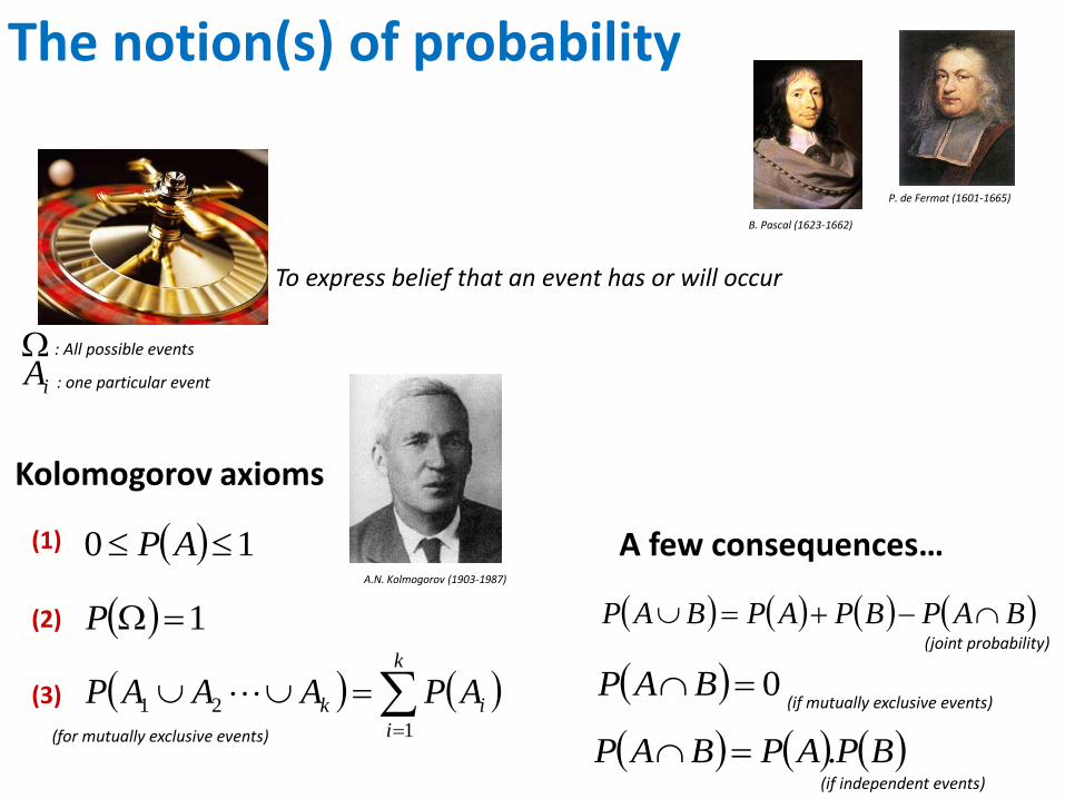
The notion(s) of probability

B. Pascal (1623-1662)

P. de Fermat (1601-1665)

A.N. Kolmogorov (1903-1987)

Kolomogorov axioms

To express belief that an event has or will occur

(1)

(2)

(3)

10 AP

1P

: All possible events

iA : one particular event

k

i

ik APAAAP1

21 (for mutually exclusive events)

A few consequences…

BAPBPAPBAP (joint probability)

0BAP

BPAPBAP .

(if mutually exclusive events)

(if independent events)

The notion(s) of probability

Frequentist interpretation Bayesian interpretation

- Probability = frequency of the occurrence of an event, given an infinite number of trials - Is only defined for random processes that can be observed many times - Is meant to be Objective

- Probability = degree of belief, measure of uncertainty - Can be arbitrarily defined for any type of event - Is considered as Subjective in essence

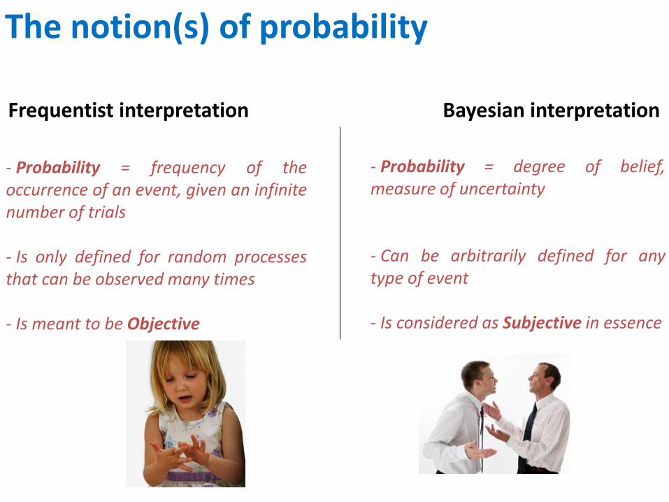
The notion(s) of probability

Frequentist interpretation Bayesian interpretation

- Probability = frequency of the occurrence of an event, given an infinite number of trials - Is only defined for random processes that can be observed many times - Is meant to be Objective

- Probability = degree of belief, measure of uncertainty - Can be arbitrarily defined for any type of event - Is considered as Subjective in essence

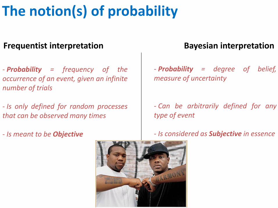
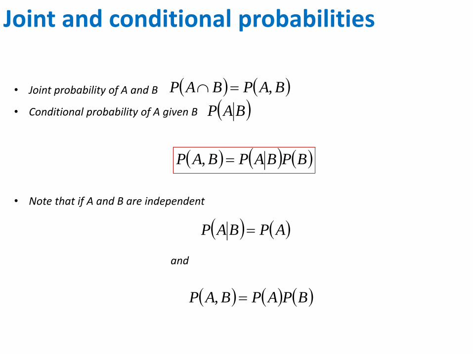
Joint and conditional probabilities

BPBAPBAP ,

BAPBAP ,• Joint probability of A and B

• Conditional probability of A given B BAP

• Note that if A and B are independent

APBAP

and

BPAPBAP ,

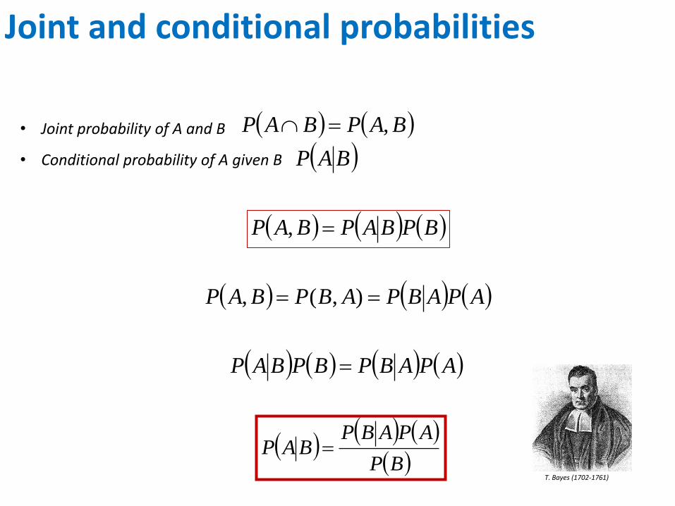
BPBAPBAP ,

BAPBAP ,• Joint probability of A and B

• Conditional probability of A given B BAP

APABPABPBAP ),(,

APABPBPBAP

Joint and conditional probabilities

BP

APABPBAP

T. Bayes (1702-1761)

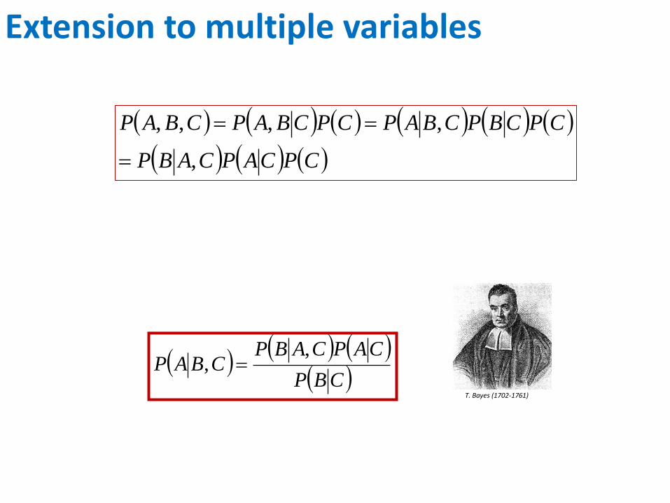
CPCAPCABP

CPCBPCBAPCPCBAPCBAP

,

,,,,

Extension to multiple variables

CBP

CAPCABPCBAP

,,

T. Bayes (1702-1761)

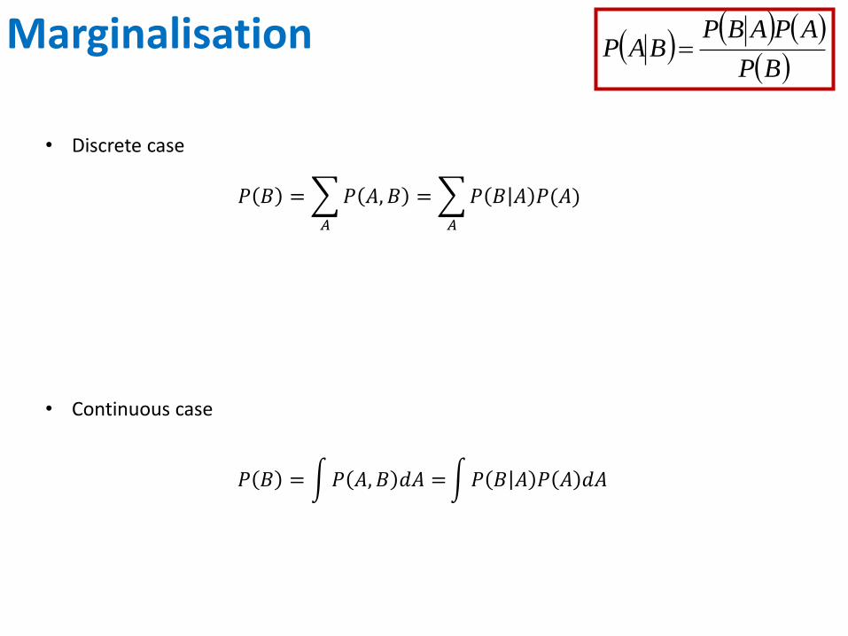
Marginalisation

• Discrete case

• Continuous case

BP

APABPBAP

𝑃 𝐵 = 𝑃 𝐴, 𝐵 𝑑𝐴 = 𝑃 𝐵 𝐴 𝑃 𝐴 𝑑𝐴

𝑃 𝐵 = 𝑃 𝐴, 𝐵 = 𝑃 𝐵 𝐴 𝑃(𝐴)

𝐴𝐴

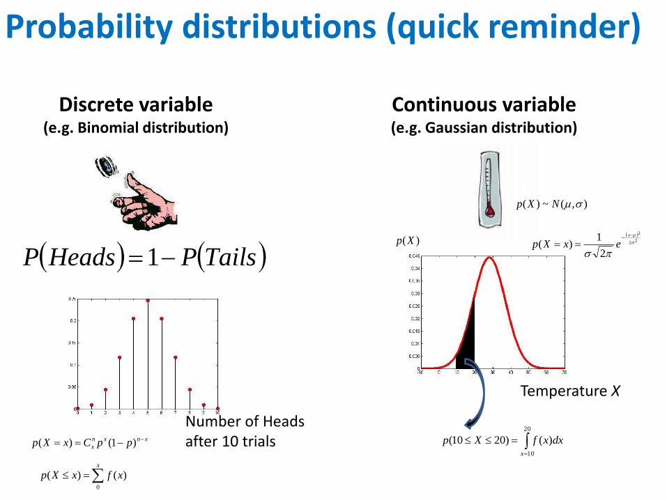
)(Xp

Temperature X

22

2

2

1)(

x

exXp

Probability distributions (quick reminder)

Discrete variable (e.g. Binomial distribution)

Continuous variable (e.g. Gaussian distribution)

TailsPHeadsP 1

),(~)( NXp

20

10

)()2010(x

dxxfXpxnxn

x ppCxXp )1()(

x

xfxXp0

)()(

Number of Heads after 10 trials

- General principles - The Bayesian way - SPM examples

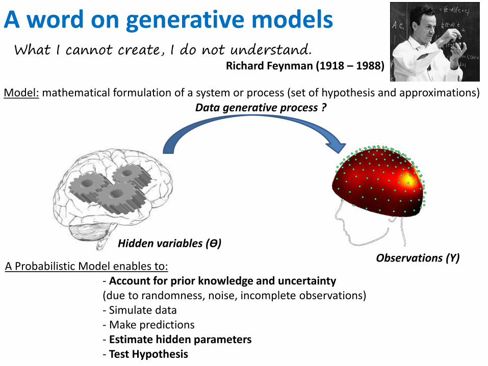
A word on generative models

Data generative process ?

Observations (Y) Hidden variables (ϴ)

Model: mathematical formulation of a system or process (set of hypothesis and approximations)

A Probabilistic Model enables to: - Account for prior knowledge and uncertainty (due to randomness, noise, incomplete observations) - Simulate data - Make predictions - Estimate hidden parameters - Test Hypothesis

What I cannot create, I do not understand. Richard Feynman (1918 – 1988)

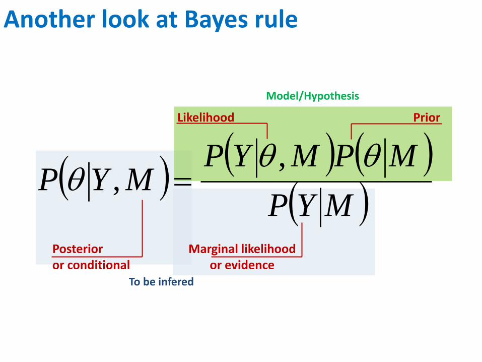
To be infered

Model/Hypothesis

Another look at Bayes rule

MYP

MPMYPMYP

,,

Likelihood Prior

Marginal likelihood or evidence

Posterior or conditional

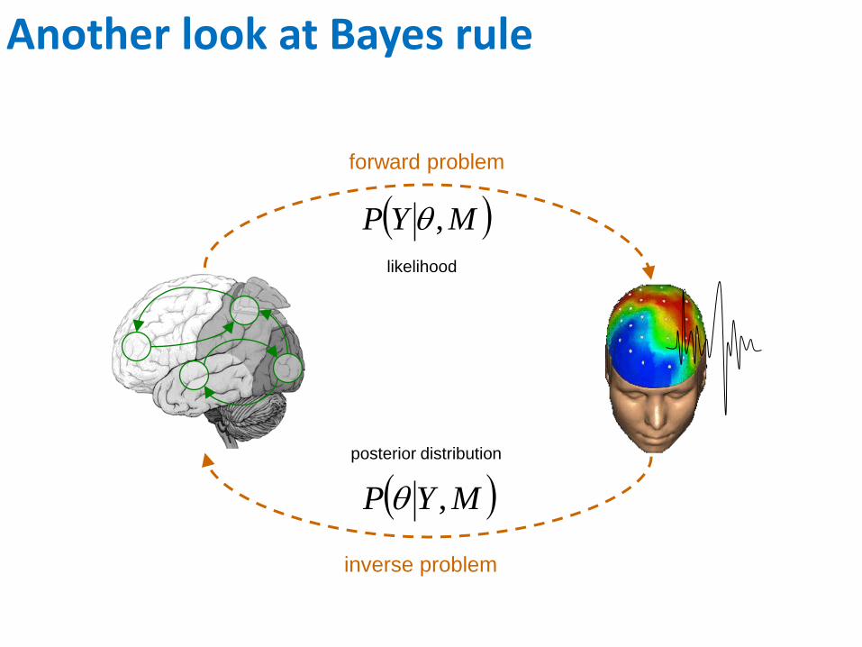
Another look at Bayes rule

forward problem

likelihood

inverse problem

posterior distribution

MYP ,

MYP ,

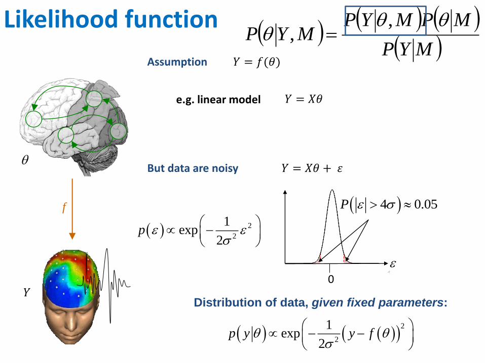
Likelihood function

Assumption

𝑌 = 𝑋𝜃

𝑌 = 𝑓(𝜃)

e.g. linear model

But data are noisy 𝑌 = 𝑋𝜃 + 𝜀

2

2

1exp

2p

4 0.05P

Distribution of data, given fixed parameters:

2

2

1exp

2p y y f

f

𝑌 0

MYP

MPMYPMYP

,,

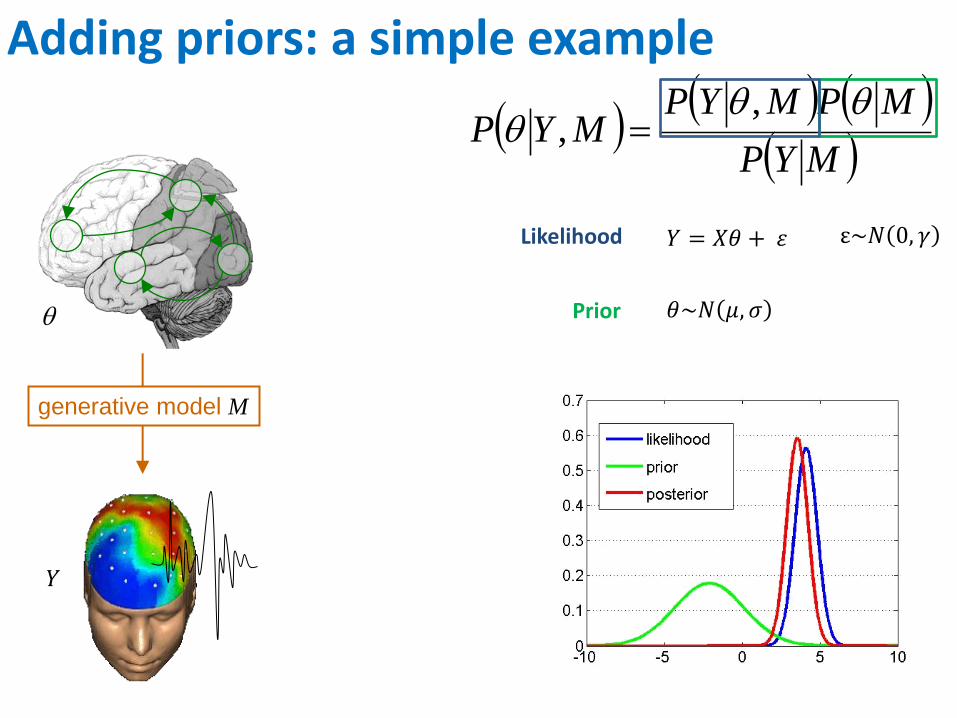
Adding priors: a simple example

MYP

MPMYPMYP

,,

Likelihood

Prior

𝑌 = 𝑋𝜃 + 𝜀 ε~𝑁 0, 𝛾

𝜃~𝑁 𝜇, 𝜎

generative model M

𝑌

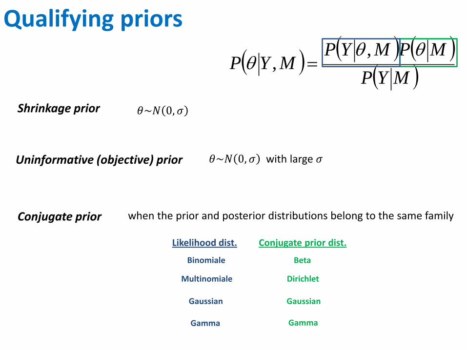
Qualifying priors

Shrinkage prior

𝜃~𝑁 0, 𝜎 with large 𝜎

Conjugate prior

Uninformative (objective) prior

𝜃~𝑁 0, 𝜎

when the prior and posterior distributions belong to the same family

Likelihood dist. Conjugate prior dist.

Beta

Dirichlet

Binomiale

Gaussian

Multinomiale

Gamma

Gaussian

Gamma

MYP

MPMYPMYP

,,

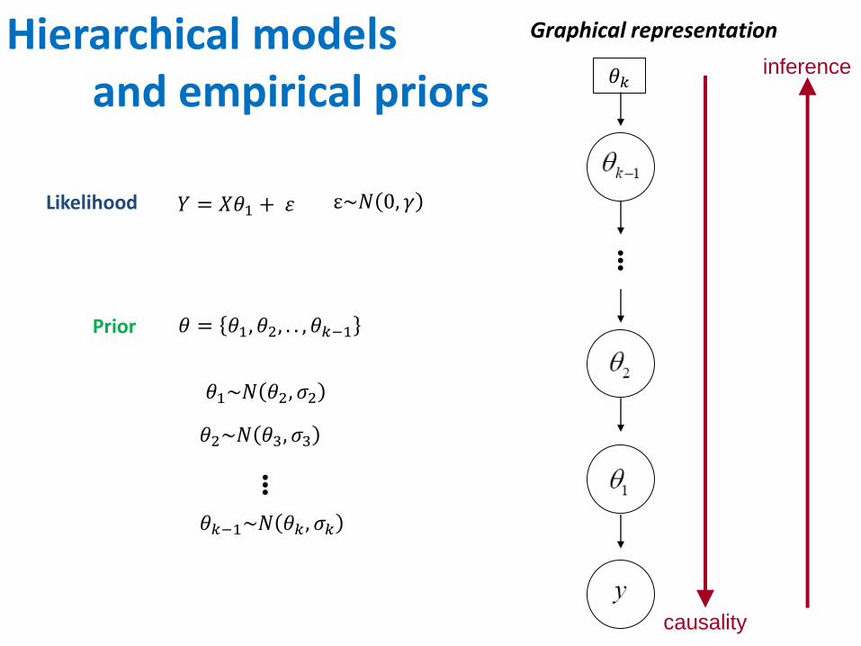
Hierarchical models and empirical priors

•••

Likelihood

Prior

𝑌 = 𝑋𝜃1 + 𝜀 ε~𝑁 0, 𝛾

𝜃1~𝑁 𝜃2, 𝜎2

𝜃 = 𝜃1, 𝜃2, . . , 𝜃𝑘−1

𝜃2~𝑁 𝜃3, 𝜎3

•••

𝜃𝑘−1~𝑁 𝜃𝑘 , 𝜎𝑘

𝜃𝑘

Graphical representation

inference

causality

To be infered

Model/Hypothesis

Another look at Bayes rule

MYP

MPMYPMYP

,,

Likelihood Prior

Marginal likelihood or evidence

Posterior or conditional

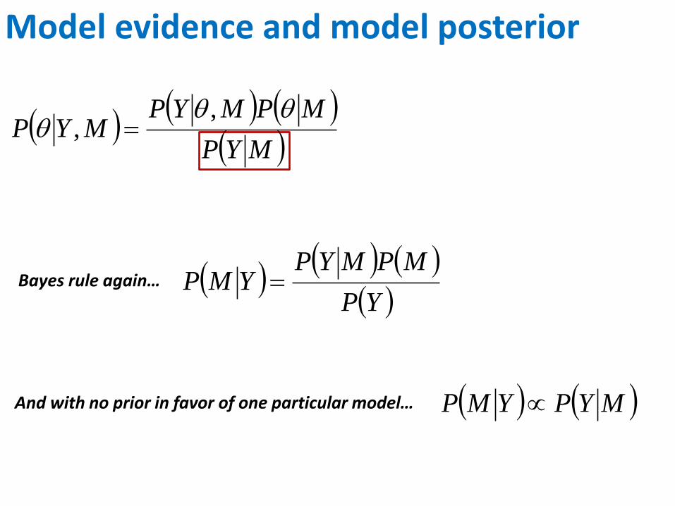
Model evidence and model posterior

MYP

MPMYPMYP

,,

Bayes rule again…

YP

MPMYPYMP

And with no prior in favor of one particular model… MYPYMP

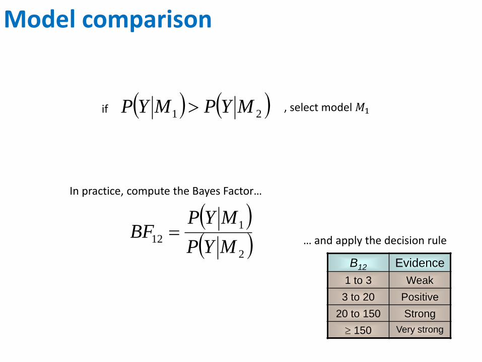
Model comparison

21 MYPMYP if , select model 𝑀1

In practice, compute the Bayes Factor…

2

1

12MYP

MYPBF

B12 Evidence

1 to 3 Weak

3 to 20 Positive

20 to 150 Strong

150 Very strong

… and apply the decision rule

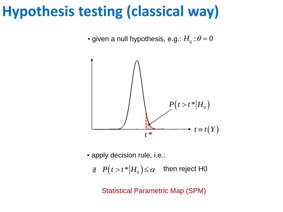
Hypothesis testing (classical way)

t t Y t *

0*P t t H

0*P t t H if then reject H0

H

0: 0• given a null hypothesis, e.g.:

• apply decision rule, i.e.:

Statistical Parametric Map (SPM)

Y

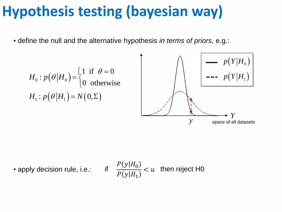
• define the null and the alternative hypothesis in terms of priors, e.g.:

0 0

1 1

1 if 0:

0 otherwise

: 0,

H p H

H p H N

if then reject H0 • apply decision rule, i.e.:

y

1p Y H

0p Y H

space of all datasets

Hypothesis testing (bayesian way)

𝑃 𝑦 𝐻0𝑃 𝑦 𝐻1

< 𝑢

Principle of parsimony

Occam’s razor

Complex models should not be considered without necessity

y=f(

x)

y =

f(x

)

x

MYP

MPMYPMYP

,,

Mo

del

evi

den

ce

Data space

dMpMYpMYp )|(),|()|(

Usually no exact analytic solution !!

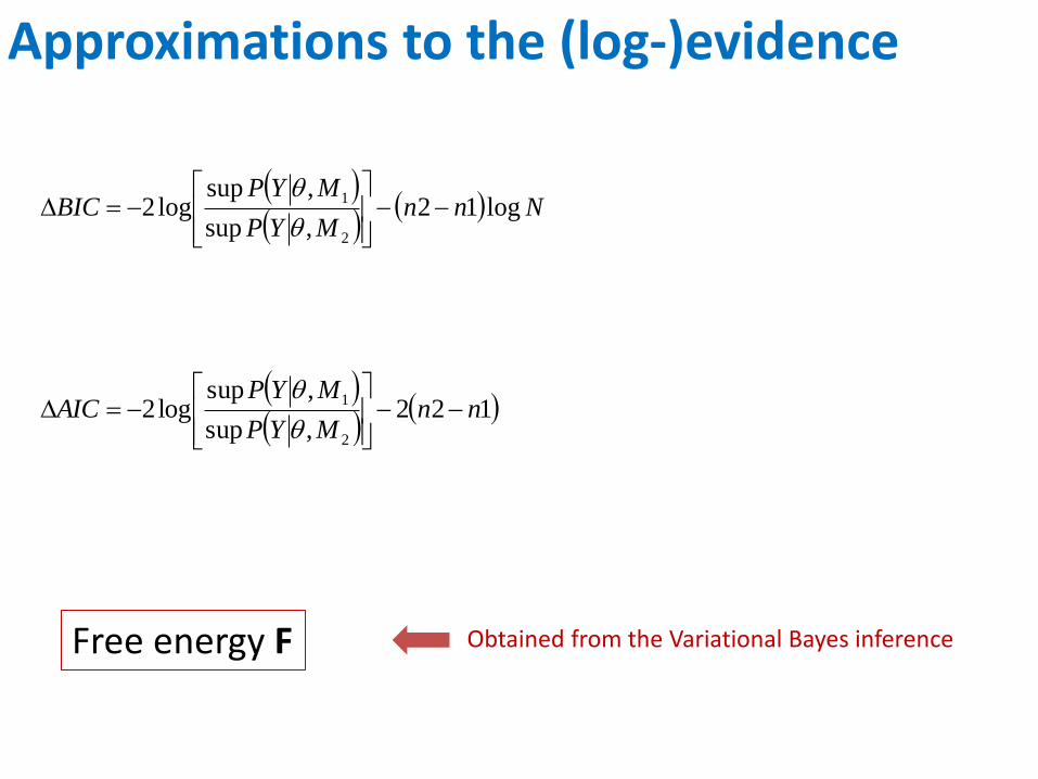
Approximations to the (log-)evidence

NnnMYP

MYPBIC log12

,sup

,suplog2

2

1

122,sup

,suplog2

2

1nn

MYP

MYPAIC

Free energy F Obtained from the Variational Bayes inference

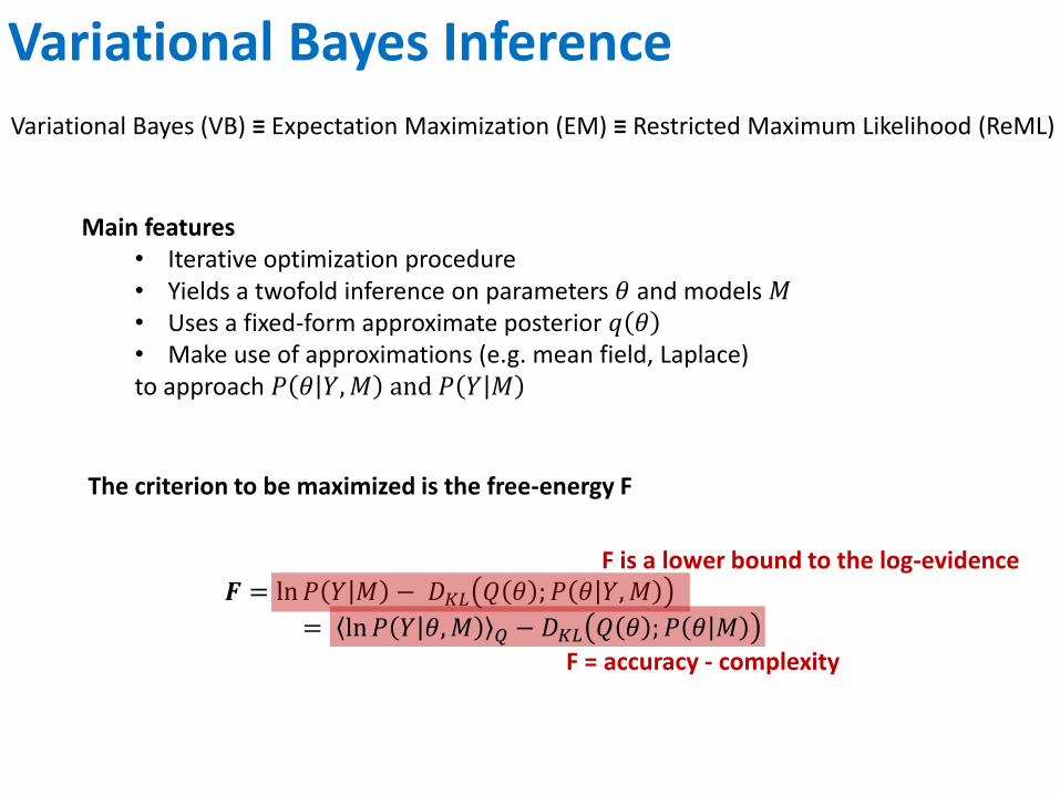
Variational Bayes Inference

Variational Bayes (VB) ≡ Expectation Maximization (EM) ≡ Restricted Maximum Likelihood (ReML)

Main features • Iterative optimization procedure • Yields a twofold inference on parameters 𝜃 and models 𝑀 • Uses a fixed-form approximate posterior 𝑞 𝜃 • Make use of approximations (e.g. mean field, Laplace) to approach 𝑃 𝜃 𝑌,𝑀 and 𝑃 𝑌 𝑀

The criterion to be maximized is the free-energy F

𝑭 = ln𝑃 𝑌 𝑀 − 𝐷𝐾𝐿 𝑄 𝜃 ; 𝑃 𝜃 𝑌,𝑀

= ln𝑃 𝑌 𝜃,𝑀 𝑄 − 𝐷𝐾𝐿 𝑄 𝜃 ; 𝑃 𝜃 𝑀

F is a lower bound to the log-evidence

F = accuracy - complexity

- General principles - The Bayesian way - SPM examples

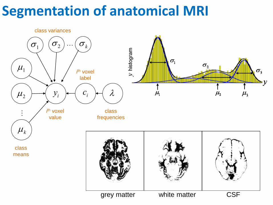
grey matter CSF white matter

…

…

yi ci

k

2

1

1 2 k

class variances

class

means

ith voxel

value

ith voxel

label

class

frequencies

Segmentation of anatomical MRI

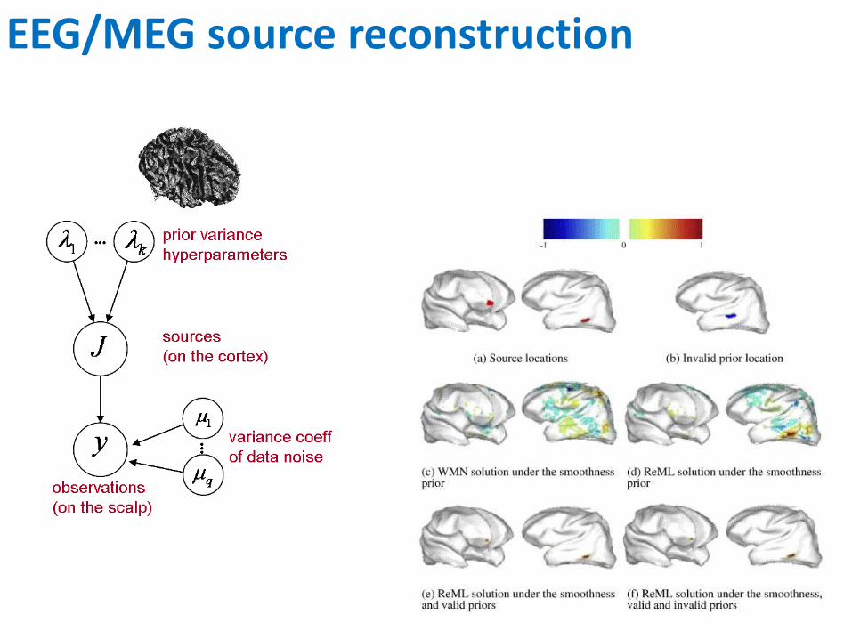
EEG/MEG source reconstruction

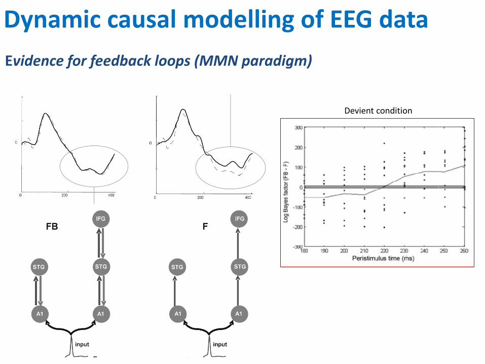
Evidence for feedback loops (MMN paradigm)

Devient condition

Dynamic causal modelling of EEG data

Suggestions for further reading