class lecture notes
TRANSCRIPT

1
Day 1: Intro to course
My teaching philosophy
• Learn economics by doing economics
• Case studies, problem sets, experiments and lab reports, exams, “naturalist” assignments,
group research projects
• Team approach
o Most important member of team = you
o Rest of us are here to facilitate your learning
o Professor
o Lab assistant
o Tutorial staff
o Q Center
o Peers
Show and discuss Web site, syllabus information
• Main page
o Class news
o My email (note no first initial)
o Links to other pages
• Course Information
o Content
o Format
Thursday activity sessions: nothing required, but good complement to rest of
course. Will try to do interesting things most weeks.
o Math prerequisites
Basic algebra, graphs, logs
Will work these methods into first homework (due next Wednesday) and
have session at second activity session to work on the math methods.
Q Center has tutorial services available specifically for math needed in non-
math course such as economics.
o Office hours
M 3-4, T 10-11, F 1-2.
Around at other times
o Tutors
Staff of three excellent tutors
Will have drop-in tutorial sessions on M and T evenings in DoJo

2
Can hire an individual tutor for up to 1 hour per week through Student
Services
o Exams and assignments
Two midterms and final, dates of midterms are on the calendar
Weekly problem sets
• Sometimes done in pairs with a partner, sometimes alone
Daily case studies
• Submit case questions by email to [email protected] before class starts
• I return comments within a couple of days
• Sometimes cases will be discussed in class; sometimes we won’t have
time. Additional form of dialog with instructor/students.
o Grading
o Texts and readings
Pindyck and Rubinfeld 6/e (not current edition)
Mankiw Principles 5/e
o Class preparation
Very ambitious agenda for the semester
Read chapter/textbook material first to get the basic idea
Do case study reading next, and answer questions
Come to class to put it all together
Ask questions if it’s not coming together
• In class
• In office hours
• By email
• At tutorial sessions
• Calendar and reading list
o Dates probably will not change much, but you never know. There is not a lot of
room for slack in the semester.
o Required readings and background readings
o Assigned work
Case of the day
Problem sets pending
• Any questions???
Economics as a social science
• Social science: use scientific method to look at human interactions (usually large groups)
• Economics: focuses on human interactions intended to solve “the economic problem:” how
best to allocate society’s scarce resources to satisfy the wants of its members.
o Take wants as given
o Resources are given in static analysis, may change in dynamic models
3
o Resource allocation as focus: who uses what to make what for whom
o Emphasis on social institutions: firms, households, markets, governments
• Microeconomics vs. macroeconomics
o Micro examines economic interactions at individual or industry level
“Trees”
o Macro looks at entire economy using summary measures, “representative agent”
“Forest”
o First 2/3 of Econ 201 is micro; last 1/3 is macro.
4
Day 2: Intro to Economics
Basic concepts
• Resources are scarce
o Labor
o Capital (human, physical)
o Land
o Entrepreneurship
• Wants are unlimited (discuss wants vs. needs)
• Economics = allocation of scarce resources to meet competing wants
o We can’t have everything we would like (airline safety)
o We must make choices
As individuals
As societies
o Economics studies how these choices
are made
are affected by public policies
are affected by social, political, and economic institutions
interact together to determine individual and social outcomes
• Positive vs. normative economics
Basic microeconomic questions
• What goods and services are produced (and in what quantities)?
o By whom is each produced?
• How are they produced?
o With what resources?
o With what technologies?
• For whom are the goods produced?
o Who gets them?
o By what rule are they allocated?
Roles of markets and centralized institutions
• These roles vary a lot across economies and goods
• Market: forum (may be physically decentralized) for exchange between buyers and sellers of
a good
• Centralized institutions: usually governments, but may include large labor unions that
allocate work among potential workers or organizations of firms that make more centralized
decisions about production (often illegally!)
5
• Traditional Communism: centralized decision-making
o Government owned most large producers
o Government planning bureaucracy decided on production quotas
o How did planners know:
How much of each good to produce?
How much of each input would be needed?
What was the best technology to use to produce it?
Who should get it?
o They often didn’t, which is why Communist systems were often very inefficient.
• Market capitalism: decentralized decision-making
o Market prices provide signals for private decision-makers, who have secure property
rights over the goods and resources that they own.
Why are property rights important?
o If lots of people want a good, it becomes more valuable, price goes up, existing firms
or new ones have greater incentive to hire resources to produce it.
o Firms have profit incentive to use most efficient available technology to produce
goods in order to minimize costs.
o If costs of resources needed for good get more scarce (oil?), then their price will rise
and good will become more costly to produce, more expensive, and consumers will
substitute away from the good.
• Market prices can be remarkably effective at allocating resources, but there are problems:
o Competitive markets allocate resources better than concentrated ones
What does competition mean?
• Lots of buyers and sellers so that everyone on both sides has many
alternative transaction partners
• This means that no single buyer or seller has power to influence the
market price on her own
o Everyone must have excellent (“perfect”) information about prices and the quality of
the goods being offered/bought.
o Property rights must often be clearly defined in order for markets to be efficient
o External costs and benefits (define) can lead private decision-makers to make
decisions that are not optimal for society
o People who own few or no valuable resources do not get access to purchasing power,
so there may be more inequality of well-being than we want.
o “Public goods” that are consumed in common by the whole society (legal system,
national defense) cannot command a price, so they may not be produced
Goal of resource allocation: efficiency
• Simple definition of efficiency = no waste
o Don’t produce things people don’t want
6
o Don’t use more resources than necessary to produce
o Use the best available technology to combine these resources
Together: be on the production-possibilities frontier: can’t produce more of
one good without reducing production of another
o Get the products to the people who want them most (e.g., don’t give a red car to
someone who likes blue and a blue car to someone who likes red: no remaining,
unexploited gains from exchange)
Pareto optimality/efficiency: can’t make one person better off without
making someone else worse off
• We will have more complex definitions of efficiency later on related to the various ways that
economies can be inefficient (productive, allocative, etc.), but this is the basic idea.
• In an efficient economy, to get more of good A (as an individual or as a society) we must
always give up something (good B). This is the opportunity cost of more A.
o (What is the opportunity cost of more airline safety?)
• Efficiency usually occurs where the marginal benefit equals marginal opportunity cost.
7
Day 3: Supply and demand
Demand curve
• Mathematical representation QD = QD(P).
o Functional notation
o Which is dependent and which independent variable???
o Decisions being represented by function
• Why does demand curve slope downward?
o Substitution
o Income depletion?
• Change in demand vs. change in quantity demanded
• Shifts in demand
o Income
o Prices of substitutes and complements
o Preferences
o Number of potential buyers
o Expectations
Supply curve
• Mathematical representation QS = QS(P).
• Why does supply curve slope upward?
• Factors affecting supply curve (Change in supply vs. change in quantity supplied)
o Cost of inputs
o Technology/productivity
o Prices of related goods
o Number of potential sellers
o Expectations
Interaction of demand and supply
• Assumptions of competitive markets
o Price takers
o Perfect information
o Instantaneous market-clearing
• Surplus or shortage
o How will price respond?
o This will bring us to “equilibrium” where S=D
8
Effects of ΔS and ΔD
• Dynamics of effect
o Initial shortage or surplus
o Response of price
• Note that size of equilibrium effect on P and Q depends on sensitivity (elasticity) of D and S
Questions for groups
Supply-Demand Questions.pptx
9
Day 4: Double-Oral Auction
Day 5: Applications of Competitive Market Model
Gains from exchange
• How much to buyers or sellers gain from transacting in the market?
o A simple way of measuring this is to compute the difference between their
willingness to pay/accept and the price they actually paid/received
• Consumer surplus
o What will most eager buyer pay for the very first unit of the good available?
Vertical intercept
o What does that person actually pay?
Marker price (start without supply curve)
o Difference is consumer surplus on that first unit.
o We can add up the little increments of surplus on each unit bought. Result is the area
under the demand curve and above the equilibrium price between zero units and the
number actually bought.
o Note that the market price signal screens buyers so that those who have the highest
willingness to pay get the good.
o Who are the people/units on the right tail of the demand curve?
Those who don’t much like the good
Those who can’t afford it
What should we do about people who love the good but can’t afford it?
• Lowering price will also attract many buyers who are rich but don’t
much want the good
• Giving the poor extra income allows them to choose which goods to
buy and brings those who really want the good into the upper part of
the demand curve.
• Producer surplus
o Same argument applies to sellers.
o Are below the market price and above the supply curve out to the equilibrium price is
gains to sellers = producer surplus.
o As with buyers, market price screens out high-cost producers and assures that the
units of the good are produced by the sellers with lowest costs (willingness to accept)
• Total gains from exchange = consumer surplus + producer surplus
• Given demand and supply curves, competitive equilibrium maximizes total gains from
exchange.
10
o Market price serves as a signal that weeds out low-value buyers and high-cost sellers
so that those with the most to gain are able to make transactions.
o It doesn’t matter who trades with whom, as long as only those who find it profitable
to trade at the equilibrium price are involved.
Effects of price control
• Suppose there is a price ceiling below the equilibrium price
o Shortage will result
o How much surplus is lost?
Depends crucially on which buyers get to buy.
Price signal no longer rations who gets the good.
Some other mechanism must ration the available units of the good
• Loudest voice? Fastest? Strongest? Luckiest? Most politically
connected?
• Note that competitive equilibrium is highly democratic: everyone
who is willing and able to buy at the equilibrium price is able to,
regardless of any possible discrimination or favoritism.
• Similar effect of price floor above the equilibrium price
Effects of taxes
• Suppose there is a tax of $T per unit on each unit sold
o Supply curve shifts upward by $T because seller needs to get $T more per unit to be
willing to sell as much as before the tax.
o Who bears the tax?
Depends on slopes (elasticities) of demand and supply curves
Steep slope bear lots of tax
Flat slope easy to adjust and avoid tax
o Show tax revenue rectangle and DWL triangle, losses to buyers and sellers
• What would be different if tax of $T was imposed on buyers instead of sellers?
o Nothing.
o Demand curve shifts down by $T and price/quantity equilibrium is same as seller
tax.
o Incidence of the tax is also the same.
• Subsidies work as negative taxes
o Do they increase surplus? Not if we subtract cost of subsidy.
o Buyers and sellers gain, but at greater cost to the taxpayers
11
Day 6: Elasticity
Definitions
• Elasticities measure the sensitivity of economic relationship.
• They are like slopes, but in some ways better.
• Sensitivity of quantity demanded to price:
o dQP
ΔΔ
is (inverse absolute) slope of demand curve
The number depends on the units that we use for Q and P
Cannot be easily compared across different products.
Nonetheless, it may be a very useful number: number of additional Reed
applicants who would come if tuition were $1000 lower.
• Elasticity measures sensitivity in terms of % changes:
o % 100 / 1% 100 /
Q Q Q Q P PE
P P P P Q slope QΔ × Δ Δ
= = = =Δ × Δ Δ
Demand elasticities
• Price elasticity of demand is negative due to “law of demand.”
o We sometimes express as absolute value since there is no question about sign
• Perfectly elastic demand: E → −∞
o Horizontal demand curve
• Perfectly inelastic demand: E → 0
o Vertical demand curve
• Elastic demand: |E| > 1
• Inelastic demand: |E| < 1
• Unit elastic demand: E= –1
• Linear demand curve has constant slope, but varying elasticity
o At top, P is large and Q is small, so P/Q is large and elasticity is large
o At bottom, P is small and Q is large, so P/Q is small and elasticity is small
• Log-log demand curve such as the one in problem set has constant elasticity equal to
coefficient on lnP.
• Income elasticity = d dI
d
Q Q IE
I I Q%Δ Δ
= =%Δ Δ
o EI > 0 for “normal goods,” EI > 1 for “luxuries” (also normal), EI < 0 for “inferior
goods”
• Cross-price elasticity = %
%Y X
Y Y XQ P
X X Y
Q Q PE
P P QΔ Δ
= =Δ Δ
o Positive for “substitutes,” negative for “complements”
12
Supply elasticity
• Supply elasticity (with respect to price) = %
%sQ
PΔΔ
• Supply elasticity is usually positive, but can be zero or infinite (perfectly inelastic or perfectly
elastic)
Point vs. arc elasticities
• Can measure QP
ΔΔ
at a single point (inverse slope of tangent line) or over an interval (inverse
slope of the chord connecting two points)
• Former is “point elasticity;” latter is “arc elasticity”
• We will use them interchangeably.
o Often easier to calculate arc elasticity from data
o Usually easier to think about point elasticity on graph
Short-run vs. long-run elasticities
• What is the short run?
o Only some things can change
o We often assume that “capital” cannot adjust
No new furnaces, cars, factories, etc. in short run
• Long run is when everything can adjust
• These definitions are very fuzzy!
• Gasoline example of short-run vs. long-run elasticities
• Reed elasticities: how will number of students change following large tuition increase?
o Many students with only one or two years left will stay
Continuing students have lower elasticity than entering students
o Fewer new students will enter
o Over time, number will decline more than immediately
• How do Reed’s price and income elasticities compare with L&C? U of O? PCC? Are other
schools substitutes? What will cross-price elasticity look like?
13
Day 7: Basic Consumer Theory • Change of focus from market interactions to determinants of underlying behavior
• From “how do supply and demand interact?” to “where do demand and supply curves come
from?”
Basic framework of consumer theory
• Assumptions about households
o They are price-takers
o They have well-defined preferences (utility)
o They behave systematically to choose more preferred to less preferred alternatives
(rationality)
Rationality is controversial
Does it matter if rationality holds perfectly? Pool player/physics example
• Method of constrained optimization
o Preferences:
Objective (utility) function represents preferences
Utility depends on amount of various goods and services (including leisure,
future goods, etc.) consumed
• Consumption is a flow: goods per year or goods per day.
o Opportunity set:
Budget constraint limits household’s choices
o We will examine the household consumption decision graphically in two dimensions
313 does using calculus, Lagrange multipliers, set theory in many dimensions
Choice space
• What are the alternatives that households could hypothetically choose?
o “Consumption bundles” or combinations of all the various consumption goods
available: (asparagus, beets, carrots, …)
o There are millions of different goods and services, especially if one includes all the
variations
o We restrict to two at a time in order to keep the graph simple
Can easily be generalized mathematically to more than two dimensions, but
it’s hard to graph in three and essentially impossible in more than three
• Suppose that we consider a household that is choosing between consumption of apples and
consumption of bananas
o The positive quadrant (including the axes) defines the choice space for the household:
the consumption bundles that could be consumed if the household could afford
them.
14
o We will consider the household’s preference function and its opportunity set within
the choice space
Preferences
• Assumptions about preferences
o Completeness: household can rank any consumption bundle with respect to any
other.
If X and Y are bundles, then either , ,X Y Y X or consumer is
indifferent between X and Y.
o Transitivity: ,X Y Y Z X Z⇒
Psychologists can often trick subjects into violating transitivity, so they are
skeptical about rationality of preferences.
Economists counter that it’s impossible to develop a theory without some
basic assumption of behavior and that the rationality assumption has led to a
reasonable and robust theory of demand.
o Non-satiation
More of a good always increases utility
• Not a critical global assumption, but probably reasonable at levels
where people actually consume
• People wouldn’t consume goods where they got negative utility from
them
• Cardinal vs. ordinal utility
o Cardinal utility attaches numbers to utility: ( ),U U A B= is utility function
Numbers are unmeasurable and arbitrary
Under cardinal utility we can think of a “utility mountain” in three
dimensions
Marginal utility is the additional utility one gets from consuming one more
unit of a particular good
o Ordinal utility requires only that we can rank alternative bundles. We don’t have to
attach a number to utility
Cardinal utility can easily be reduced to ordinal, so ordinal is less restrictive
assumption
All of utility theory can be derived from ordinal preference rankings, so we
usually don’t use cardinal
• Indifference maps
o Look at two goods at a time (sometimes make one “other stuff” to represent
everything other than the good we are modeling)
Bananas on vertical, apples on horizontal
15
o With cardinal utility, we can think of indifference curves as the “contour lines” of the
utility mountain
o Points up and to the right are preferred to those down and left (by non-satiation)
Draw preference arrow
o There is one indifference curve through every point in the space
o Indifference curves cannot intersect
o Indifference curves for
perfect substitutes
perfect complements
ordinary pairs of goods (convex)
• Marginal rate of substitution
o MRS = –slope of indifference curve = BA
Δ−Δ
= number of bananas the consumer is
willing to sacrifice to obtain one additional apple, keeping her at same level of utility.
Show rise over run on graph with run = 1
o MRS reflects willingness to trade one good for the other
o “Law” of diminishing MRS reflects the fact that one’s preference for more of
something declines as one has more of it (relative to other goods)
If one has 10 bananas and one apple, one is probably willing to exchange
several bananas for another apple.
If one has 10 apples and one banana, one is probably willing to exchange
several apples for another banana.
Addictive goods?
Opportunity sets
• If household has fixed income I and is a price-taker, then it can choose A and B subject to the
budget constraint .A BP A P B I+ ≤
o Solving budget constraint for B: .A
B B
PIB A
P P≤ −
o The boundary condition (equality part of ≤) is a line with vertical intercept at I/PB
and slope –PA/PB (and horizontal intercept at I/PA.
o Opportunity set is a triangle with axes and boundary line segment
• Increase in income: budget constraint shifts parallel outward
• Increase in PA: horizontal intercept moves toward origin with no change in vertical intercept;
curve gets steeper
• Increase in PB: vertical intercept moves toward origin with no change in horizontal intercept;
curve gets flatter
• Equi-proportional increase in income and both prices: no change in budget constraint
16
Consumer equilibrium
• What is the highest level of utility (most preferred point) that consumer/household can reach
within its opportunity set?
• Two possibilities:
o Interior solution
Tangency between indifference curve and budget line
Slopes of indifference curve and budget line are equal
• MRS = –PA/PB
• Marginal benefit of one more apple (MRS) = marginal cost (relative
price)
o Corner solution
If indifference curve is flatter than budget line at vertical axis, then consume
none of the horizontal good.
If indifference curve is steeper than the budget line at horizontal axis, then
consume none of the vertical good.
17
Day 8: Income and Substitution Effects
Effects of change in price
• Put “other goods” on vertical axis to focus on single good.
o Let price of “other goods” be normalized to one.
o Vertical intercept is just income (divided by one)
• Increase in price of good A pivots budget constraint around vertical intercept, making it
steeper.
o Show price-consumption curve
o Translate to demand-curve space
o Note that this is demand for A by individual household
o Aggregate households horizontally to get market demand curve
( ) ( ), ,... , ,...d d di i
i
Q Q P I Q P I= =∑
Effects of change in income
• Parallel shift in budget constraint
• Show income/consumption path and how it translates to demand-curve space as shifts in
demand curve at constant price.
• Note difference between normal and inferior goods
Income and substitution effects
• Consider increase in the price of A
• Two effects on budget line:
o Gets steeper
o Shifts left (around vertical intercept)
• Show effects on graph
o a → b = substitution effect
o b → c = income effect
• Substitution effect is always in opposite direction of price change
• Income effect depends on whether good is normal or inferior
o Negative real income change means effect on consumption is negative for price
increase for normal good.
o For normal good, income effect reinforces substitution effect
o For inferior good, income effect counteracts substitution effect
Can income effect ever outweigh substitution effect?
Giffen good would have upward-sloping demand curve
Theoretically possible, but no convincing examples
18
Social effects on consumption?
• Bandwagon effects (fads)
o Increase in aggregate Q increases individual demand, given price.
o ( ),di iQ D P Q
+=
o Network externalities may lead to “rational” bandwagon effects
Telephones, fax machines, email, money, language, etc. are more useful the
more other people use them
• Snob effects
o Increase in Q decreases individual demand, given price
o Examples?
Group quiz on consumer equilibrium
19
Day 9: Consumer Decisions under Uncertainty
Nature of economic uncertainty
• To this point, we have assumed that there is no uncertainty (risk) in economic life.
• Households can choose exactly what combination of goods and services they want, given
their budget constraints.
• Many decisions involve uncertain outcomes
o Attending Reed
Will you succeed?
Will you be able to prepare yourself for future success?
o Tickets for an outdoor event
Will it rain?
o Lotteries, gambling, insurance
All involve increasing or reducing risk
Modeling uncertain outcomes
• Usually done in terms of income equivalent, but can be done as goods
• Usually done with cardinal utility function of income
• Expected value
o Average outcome across infinitely many trials
o Sum of possible outcomes, weighted by probabilities of occurring
• Variance
o Measure of how much and how far the outcome is likely to deviate from the
expected value
o High variance = high risk
Utility functions and risk
• Consider the utility function u(I)
• Marginal utility is value in utility terms of additional income
• Is MU increasing, constant, or decreasing with income? (Show graphs, MU = slope)
o When would you value $1000 increase in income more, when you are earning
$10,000 or when you are earning $1,000,000?
o Typical economic assumption is decreasing MU as income gets higher
• Since people don’t know their actual utility outcome, we often assume that they maximize
expected utility.
• Decreasing MU implies risk aversion
o 50/50 chance of winning or losing $5000 is unattractive because loss hurts more than
win helps
20
o Show on graph: u(10000) vs. average of u(5000) and u(15000)
o If MU is decreasing with income, then people will be risk averse.
Examples of market involving risk
• Financial investments are always risky
o Ideal asset: high return and low risk
o These assets will be so valuable that their price will be bid up.
Given their expected dollar returns, a higher price means a lower rate of
return per dollar invested
o In equilibrium, the returns on low-risk assets will be bid down below the returns on
high-risk assets
Investors will face a tradeoff between low-risk-low-return assets and high-
risk-high-return assets
Example: Treasury bills vs. junk bonds
• Insurance markets
o Why do people buy insurance?
• Lotteries and gambling
o Why do people buy lottery tickets?
o Do the same people buy lottery tickets as buy insurance? Why?
Behavioral economics
• Section 5.5 on behavioral economics discusses situations in which the “rational consumer”
model does not seem to work well
• People in experiments (and real world?) value loss of item more than gaining same item
• People in experiments (and real world?) seem to value “fairness” while “rational” consumer
would not.
• People do not always apply the laws of probability correctly, or have accurate perceptions of
true probabilities (safety of driving vs. flying)
21
Day 10: Production
Production functions
• Assume (for simplicity) that a firm produces only one output, measured by q
• Firm uses two inputs or factors of production (again, for simplicity), labor L and capital K. o We can think of output as “value added” in order to eliminate the role of intermediate
inputs of materials • Adding more inputs leads to more output • Production mountain rising from origin
o Can slice this production mountain in several directions o Slicing horizontally gives “isoquants”
Like indifference curves except they give different combinations of labor and capital that can be used to produce a given quantity of output
Unlike indifference curves, there is a clear cardinal magnitude associated with each isoquant: q
o Can slice at a given value of K Gives the production function relating q to L at given level of K
Fixed and variable factors of production • Fixed factors cannot be adjusted in the short run, but are flexible in the long run • Variable factors are flexible in the short run and the long run • We will assume that K is a fixed factor and L is a variable factor
o This is not necessarily realistic o There are many kinds of labor that are probably fixed over some horizons
Reed’s faculty is on yearly contracts Dairy farmer’s family members who work on the farm
o There are also some kinds of capital that can be easily varied in the short run More computers can be obtained in a few days
o The key point is that there are fixed and variable factors, not the labels we attach to them in our class discussion
• The short-run production function is ( ) ( ),q F K L f L= = with K fixed in short run
Total, average, and marginal product of an input
• Total product = q
• Average product = q/L
• Marginal product = ΔQ/ΔL
• How do these vary as L changes (for given K)?
• Draw TP, AP, and MP functions showing MP cutting AP from above at max
o MP initially increasing, then decreasing
• Law of diminishing marginal returns
22
• Effects of increase in K
• Effects of technological progress
Isoquants and long-run production
• In long run, we can choose both K and L
• Isoquants are contour lines of production mountain
• Substitution among inputs
o We will use this diagram to describe how firms choose the cost-minimizing
combination of factors to produce any particular level of output.
• MRTS = –ΔK/ΔL = MPL/MPK
• Substitute and complement factors
Returns to scale
• Constant returns to scale: 10% increase in all factors of production raises output by 10%
• Increasing returns to scale: 10% increase in all factors of production raises output by more
than 10%
• Decreasing returns to scale: 10% increase in all factors of production raises output by less
than 10%
o Distinguish from diminishing marginal returns
23
Day 11: Cost Curves
Key cost concepts
• Economic cost: opportunity cost vs. accounting cost
o Tuition and forgone earnings (or leisure) are economic (opportunity) cost of
attending Reed
Tuition is accounting cost, but forgone earnings are not
o Room and board is not an opportunity (economic) cost because you would have to
live and eat anyway
They are accounting costs
o Most common application of opportunity cost in production:
Resources owned by a firm for which it pays no accounting cost, but incurs
the opportunity cost of not selling or renting them to someone else
Building with great location: PPS and Blanchard Building
Brilliant ideas: can use or license patents
o Does it cost me less to grade my own homework assignments than to hire a student?
• Sunk cost
o If cost is already committed and can’t be recovered, then the cost is “sunk” and the
opportunity/economic cost is zero.
Reed tuition for this semester is now a sunk cost
Economic cost of the remainder of the semester is only the forgone earnings
(or leisure, if that is better)
o Be particularly careful about these costs before they are sunk
o Once they are sunk, they are irrelevant
• Variable vs. fixed costs
o Costs associated with variable and fixed factors
o Fixed costs are variable in the long run
Sunk costs are not variable even in the long run because they cannot be
recovered
Which of Reed’s costs are fixed vs. sunk?
• MC questions about sunk and economic costs
Costs in the short run
• TC
• FC and VC
• Average cost: ATC, AFC, AVC
• Marginal cost: MC
• Describe each conceptually, then show dairy farms table, use Excel to calculate.
• Show usual shapes of curves
24
Costs in the long run
• No fixed cost
• What is the cost of capital goods? (Remind of definition of capital)
o “User cost” or “rental price” of capital
o Includes (economic) depreciation of capital during the period of use
o Includes forgone interest because owner of capital had money tied up in capital good
and could not earn interest by lending it out
o Per dollar of capital: user cost = r = depreciation rate + interest rate
Per machine user cost = PK × r
o User cost = rental rate because owner of capital can choose between using and
renting out
o Easiest to think of firm as renting capital, so rental rate in terms of cost of one unit of
capital = r
• Choice of input combination: minimizing cost of producing q
o Iso-cost lines: C wL rK= + or C w
K Lr r
= −
o Straight line with slope –w/r
o Given isoquant for chosen level of q, lowest cost technology is where lowest iso-cost
possible line touches isoquant, which occurs at tangency.
o At tangency: MRTS = slope of iso-cost line, so MPL/MPK = w/r, or MPL/w =
MPK/r
This means that the additional output from spending a dollar on labor =
additional output from spending a dollar on capital.
Must be true for firm to be cost minimizing
• Costs and output in the long run
o SAC = short-run ATC
o Graph SAC curves corresponding to various levels of capital input
o LAC is envelope of these SAC curves
o LMC is marginal cost curve corresponding to LAC (and LTC, which we don’t draw)
o Economies of scale and diseconomies of scale
(Read sections on multiproduct firms, learning curves, and measurement of economies of scale for
interest, but we will not cover.)
25
Day 12: Perfect Competition in Short Run
Nature of perfect competition
Competition and monopoly are black and white.
There is no black and white, only shades of gray.
But gray is hard to analyze, so we often pretend that dark grey is actually black and light gray is
white.
• Price takers
• Homogeneous product
• Free entry and exit
• Perfect information
Profit and profit maximization
• Economic profit = revenue – economic cost
• Owners will want maximum profit
o Will managers also want this?
o Principal/agent conflicts are possible
• Evolutionary argument for profit maximization
o Those who do it survive, those who don’t are driven from market
• Social implications?
o If we can count on producers to maximize profit, we can try to design system to
harness that objective to serve general benefit
Basics of profit maximization
• ( )TR R q Pq= =
o Show TR curve
o Show TC curve
• ( ) ( ) ( )q R q C qπ = −
o Tπ curve as difference
o Show profit maximizing point
o MR = MC
Profit max under competition
• Perfectly elastic demand curve = price taker
• ( )R q Pq=
26
• TR curve is linear
• MR is horizontal at P
• Show short-run MC, ATC, AVC, with P = MR
• Shut-down rule
o P > min AVC, then produce
o If you can cover variable costs, keep producing
o If you can’t, shut down
• Competitive firm’s supply curve is MC curve above min AVC
• Competitive industry’s supply curve is horizontal aggregation of firms’ supply curves
Short-run equilibrium in competitive industry
• The givens:
o Preferences of every potential consumer (indifference map)
o Income of all consumers and prices of all other consumer goods (budget constraint, if
we knew the price of the good)
o Production function of every potential producer of the good
o Prices of all inputs to production
• From indifference maps, income, and prices of other goods
o Derive each individual consumer’s demand curve
o Aggregate horizontally to get downward-sloping market demand curve
• From production function and input prices
o Derive each individual producer’s cost curves
o Individual producer’s supply curve is MC above AVC
o Aggregate horizontally to get (usually) upward-sloping short-run market supply
curve
• Market demand and supply curves determine equilibrium market price (and quantity)
• We can determine production of individual firms and consumption of individual households
from their supply and demand curves, or by going back to the cost and indifference diagrams
that created them.
• We can do comparative experiments with changes in the underlying givens:
o Change in preferences for the good (or income or in price of complement or
substitute in production)
o Change in technology (affects cost curves through production function)
o Change in input prices (affects cost curves directly)
27
Day 13: Perfect Competition in the Long Run
Long run differs from short run in two ways:
• Firms can adjust fixed inputs
• Firms can enter or leave industry
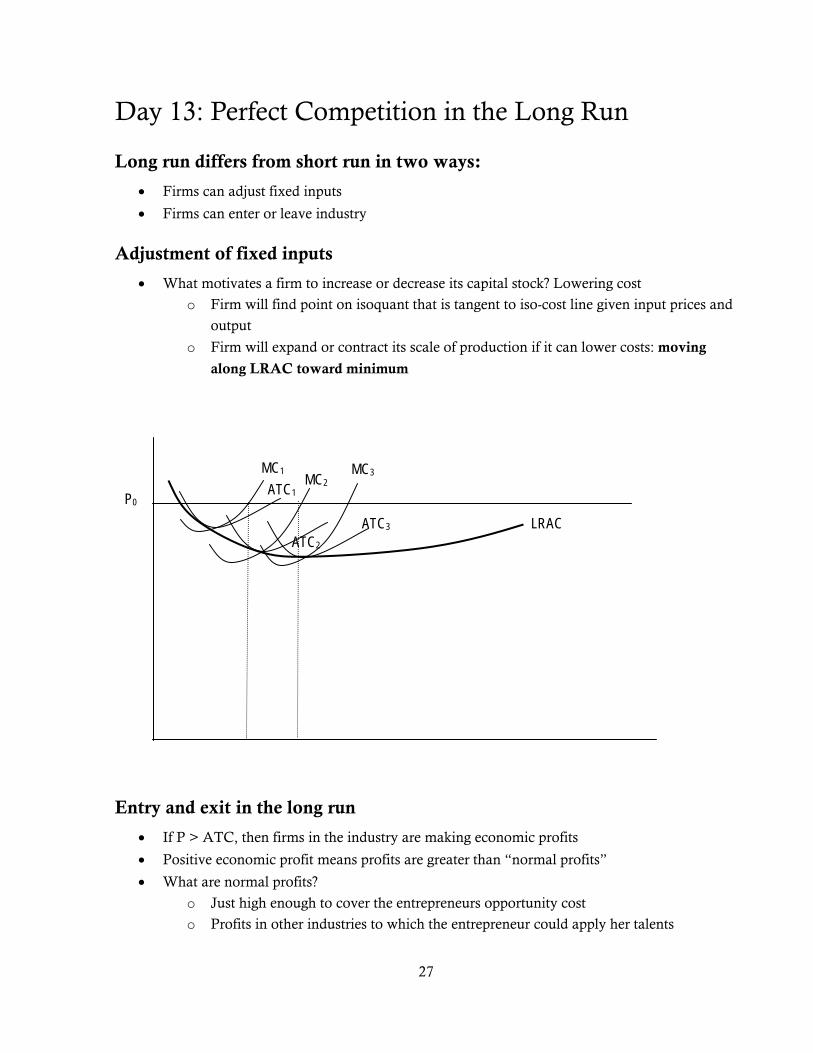
Adjustment of fixed inputs
• What motivates a firm to increase or decrease its capital stock? Lowering cost
o Firm will find point on isoquant that is tangent to iso-cost line given input prices and
output
o Firm will expand or contract its scale of production if it can lower costs: moving
along LRAC toward minimum
Entry and exit in the long run
• If P > ATC, then firms in the industry are making economic profits
• Positive economic profit means profits are greater than “normal profits”
• What are normal profits?
o Just high enough to cover the entrepreneurs opportunity cost
o Profits in other industries to which the entrepreneur could apply her talents
P0 ATC1
MC1
ATC2
MC2
ATC3
MC3
LRAC
28
o Normal profits are part of costs: the opportunity cost of entrepreneurial input plus
normal (market) returns on invested capital
• Positive economic profit means that profits are higher in this industry than in others
o This will attract new firms to enter the industry (recall free entry assumption)
o New firms will continue to enter the industry as long as economic profit > 0
o If firms are making losses, then exit will occur
• Entry into industry means more firms MC curves above AVC will be added into the short-
run market supply curve
o Short-run market supply curve shift to the right, lowering price
Long-run equilibrium in competitive industry
• Expansion or contraction of capital stock pushes firms to minimum of ATC
• Price must fall (or rise) until economic profit = 0
o P = ATC
• Long-run equilibrium price = min LRAC
• Characteristics of long-run equilibrium
o All firms are maximizing profit where P = MC
o All firms are minimizing cost at min of ATC and LRAC
o All firms are earning zero economic profit
o S = D
• Differential profits due to “economic rents”
o What if one firm has best farmland and can produce more than others?
Could it sell or rent that farmland?
The “profit” that the firm seems to earn is actually “economic rent” on the
super-productive farmland.
The opportunity cost of using this land includes the rent, so these are part of
economic cost and not economic profit.
Long-run supply curve
• Constant cost industry: horizontal LR supply curve
o Trace effects of ΔD on market in SR and LR
o Increased output will imply more inputs being used by industry
• Increasing cost industry: As production goes up, prices of inputs get bid upward
o This will raise LRAC of each firm and cause LR equilibrium price to increase as
more is produced by industry
• Decreasing cost industry: Economies of scale in inputs?
29
Day 14: Analysis of competitive markets Chapter 9 has lots of comparative analyses: taxes, subsidies, price floors and ceilings, international
trade, etc.
Efficiency
• An efficient market maximizes gains from exchange for buyers and sellers collectively
o Note producer surplus = π + FC in SR
• Perfect competition seems to lead to efficiency because surplus is maximized
• Key condition for efficiency: P = MC
o Price represents the value that consumers place on the marginal unit of the good
o MC represents the cost of the resources required to produce the marginal unit of the
good
o If P > MC, then economy should produce more of it because value to consumers
exceeds opportunity cost of resources required
o If P < MC, then economy should produce less of it because value to consumers is
less than opportunity cost
o P = MC is therefore the optimum level of consumption
• Perfect competition leads to P = MC.
• Potential problems:
o Externalities: What if private MC ≠ social MC?
Pollution is negative externality.
Firm will not consider external cost, so too much might be produced
Can have external benefits in other situations
o Imperfect information
Incorrect perception of product quality can lead to poor decisions
Policy-related inefficiencies
• Recall examples we have already done
o Price ceiling in double-oral auction
o Price supports and subsidies in Problem Set #1
o Tax examples in class when we did consumer and producer surplus
• Washington sales tax
o Is retail industry roughly competitive?
o Washington producers have higher costs than Oregon producers because of tax
o Show Washington and Oregon equilibria if border closed (short run S)
o What will happen when border opens?
Will Washington buyers buy in Oregon?
Will Oregon buyers buy in Washington?
o Long-run equilibrium: Constant-cost industry?
30
o High-value/low transportation cost Washington firms leave market
o Low-value/high transportation cost separate markets persist
o Differentiated good separate markets can exist
o Restriction on cross-border purchases (licensing of cars, delivery of furniture) may
keep markets separate as well.
• Subsidy
o Deadweight loss triangle
o Cost to government
• Price ceiling
o Deadweight loss is at least the usual triangle
• International trade
o Basic diagram with imports or exports making up surplus or shortage
o Non-prohibitive tariff (World price + tariff < domestic equilibrium)
o Prohibitive tariff
o Example: Sugar quotas on p. 325.
31
Day 15: First midterm
Day 16: Monopoly • Monopoly = single seller
• Monopsony = single buyer
• Analysis is relatively symmetric, but monopsony is less common than monopoly, so we
focus on monopoly
• Monopoly is the black corresponding to perfect competition’s white: most of the world lies in
the gray area between
• Where does monopoly power come from?
o Barriers to entry prevent others from entering
o Control of unique resources, patents, legally protected monopolies
o Differentiated product can carve out unique mini-monopolies for each firm
Monopolistic competition
o Economies of scale that persist beyond total market demand
Basic analysis
• For competitive firm, MR = AR = P because the firm sells at the same price no matter how
many units it sells.
o Competitive firm faces horizontal demand curve at market price
• Monopoly faces full market demand because it is the only seller; demand curve slopes
downward.
o In order to sell additional units, monopoly must lower price
o We assume (for now) that the monopoly must sell all units at the same price and
cannot price discriminate
• AR = P = demand curve
• Since AR is falling, MR must lie below
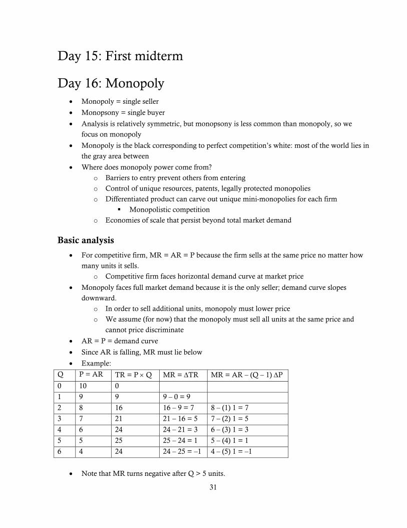
• Example:
Q P = AR TR = P × Q MR = ΔTR MR = AR – (Q – 1) ΔP
0 10 0
1 9 9 9 – 0 = 9
2 8 16 16 – 9 = 7 8 – (1) 1 = 7
3 7 21 21 – 16 = 5 7 – (2) 1 = 5
4 6 24 24 – 21 = 3 6 – (3) 1 = 3
5 5 25 25 – 24 = 1 5 – (4) 1 = 1
6 4 24 24 – 25 = –1 4 – (5) 1 = –1
• Note that MR turns negative after Q > 5 units.
32
o This is the inelastic part of the demand curve where the %Δ in Q is smaller than the
%Δ in P, so PQ goes down when Q goes up.
o Profit maximizing monopoly (with non-negative MC) would never produce on
inelastic part of demand curve
With linear demand curve, the inelastic part is the bottom half
• Show two vertical diagrams with TR & TC, AR & MR & MC.
o Decision rule: produce quantity where MR = MC (assuming greater than AVC).
o Price at the level allowed by the demand curve
o Note that P > MC for monopoly (inefficient)
• There is no “supply curve” for monopoly because it is not a price-taker.
o The question “how much will they produce and sell if the price is X?” is not well-
posed because they set price and quantity together.
• MR=MC pricing rule implies that the markup percentage = 1
d
P MCP−
=ε
o The more monopoly power, the smaller the elasticity of demand (though it’s always
elastic so that MR > 0), and the larger is the markup.
Social cost of monopoly power
• Competitive markets are efficient (absent externalities) because P = MC
• Monopoly produces where P > MC
• “Triangle” above MC and below demand curve is lost surplus due to the “contrived scarcity”
of monopoly.
o MC represents the opportunity cost of the resources required to produce marginal
unit.
This is supply curve in hypothetically competitive industry
o Rectangle between competitive and monopoly prices is also transferred from buyers
to the monopoly seller.
• Monopoly profit can be determined if we add in ATC
• Social cost of monopoly can be even higher if they dissipate some of their profits in rent-
seeking.
Regulation of monopoly
• Setting price ceiling for monopoly good makes D have horizontal segment from regulated
price to axis.
o MR is also horizontal along this segment, then jumps down to normal MR curve
• If regulation is effective, then MR hits MC on the vertical part, to the right of the usual
monopoly equilibrium.
• More is produced and efficiency costs are lower.
33
• Problem with regulation is information: knowing the monopoly’s cost and demand curves so
that the regulator can set appropriate regulatory price
Natural monopoly
• Show diagram with ever-falling LRAC and LMC below
• Show Qm, Qc, and Qb
• What is optimal regulation?
o Let them produce monopoly amount?
o Limit to break-even point?
o Subsidize to produce efficient quantity?
What efficiency costs will be involved in collecting the taxes that are needed
in order to subsidize?
34
Day 17: Price discrimination and monopolistic
competition Do monopolistic competition first, then price discrimination and other monopoly topics as there is
time.
Monopolistic competition
• Elements of perfect competition and elements of monopoly
o Free entry and exit like competition
o Differentiated (heterogeneous) product gives some (limited) monopoly power
Fairly close, but not perfect, substitutes are available
Retailers’ locations or brand loyalty may give this amount of power
• Short-run diagram is like monopoly
• If π > 0, then there is entry in long run
o Entry shifts the firm’s demand curve downward (and might make it more elastic)
• In long run, demand curve shifts until it is tangent to ATC curve.
o Demand curve is still downward-sloping, so this happens to left of min ATC (and
min LRAC)
Firms have “excess capacity” and would lower ATC by producing more
o P > MC, so there is still inefficiency
o But firms are not making economic profits (due to free entry)
• Monopolistic competition became less popular in micro but more popular in macro, as
macroeconomists learned to build mathematical general-equilibrium models where firms are
monopolistically competitive.
o Econ 314 uses these models heavily.
Price discrimination
o First-degree
o Charge every customer his or her “reservation price”
o Usurps all consumer surplus to the producer
o But socially optimal quantity is produced because MR = P = MC
o How would a firm separate the market so effectively and know everyone’s
reservation price?
o Is Reed’s financial aid 1st-degree price discrimination?
Only partially because we base on ability to pay, not on willingness to pay
o Second-degree
o Discriminate according to quantity bought
o Quantity discounts and block pricing schemes
o Third-degree
35
o Segmented market
o MR1 = MR2 = MC
o 1 2
2 1
1 1/11
1 1/
PMR P
P+ ε⎛ ⎞= + ⇒ =⎜ ⎟ε + ε⎝ ⎠
o More elastic market gets lower price
o Coupons, rebates, and airline advance-purchase discounts as 3rd-degree price
discrimination
o Intertemporal price discounts
Charge high price to eager initial buyers, then lower price to get rest of
market
Hard-cover vs. paperback books
Peak-load pricing
o For non-durable goods and services
o Price high at peak because elasticity is low?
o Or maybe MC is very high at peak (electricity generation) and low off peak?
o Examples: ideal electricity pricing, happy hour discounts, hotel and airline rate variations
Two-part tariff pricing
o Two fees: “entry fee” up front and “usage fee” for each use
o Printers and ink cartridges
o Cell phones and monthly service
o Game systems and games
o Demand is less elastic after initial subscription purchase is made, so prices on use can be
higher than the up-front charges
Bundling of goods
• When demand for two goods is somewhat negatively correlated, can use bundling to lower
price of less desired good for each kind of customer.
• Example: GPS and DVD player in minivans
o Some want GPS, will add on DVD if together
o Some want DVD, will add on GPS if together
Advertising
• No advertising in competitive market (why?)
• What does advertising do?
o Increase demand
o Lower demand elasticity
• Marginal benefit of advertising = increased sales and revenue
36
• Marginal cost of advertising
o Direct cost of advertising
o Cost of producing the additional output
• Should advertise up to the point where marginal benefit = marginal cost
37
Day 18: Oligopoly
Nature of oligopoly
• Few firms selling in a market
• At least some firms are large enough to influence market price
o Good may be homogeneous or differentiated
• Barriers to entry that allow some economic profit to persist in the long run
• Key attribute of oligopoly is strategic interaction of firms
o Firm A is large enough that other firms will react to its decisions
Firm A must take these reactions into account in determining its optimal
actions
o This doesn’t happen in competition because all firms are too small to be noticed
o This doesn’t happen in monopoly because there is only one firm
o Higher education market?
Reed is not oligopolistic because it is so small and has so many “rivals” that
no one is likely to react to its decisions
Harvard, Princeton, Stanford, Yale may be oligopolistic because they are a
small group that has a distinct market position and watch each other closely
U of Oregon, Oregon State, and Portland State would be oligopolistic if they
were independently run because they are the big players in a clearly defined
market for in-state Oregon students
o Strategic interaction is a defining characteristic of oligopoly
o The analysis of strategic interaction is game theory
• We will focus mostly on duopoly, but the general theories can be extended to more than two
firms.
Nash equilibrium
• The basic form of equilibrium in game theory is Nash equilibrium (John Nash, subject of A
Beautiful Mind)
• Each agent formulates a strategy to react to its rival’s decisions: reaction function
o ( ) ( )1 1 2 2 2 1,X f X X f X= =
• Nash equilibrium occurs where each player is making an optimal decision given the other
player’s decision
o ( ) ( )1 1 2 2 2 1* * , * *X f X X f X= =
Cournot oligopoly
• Two firms producing homogeneous product
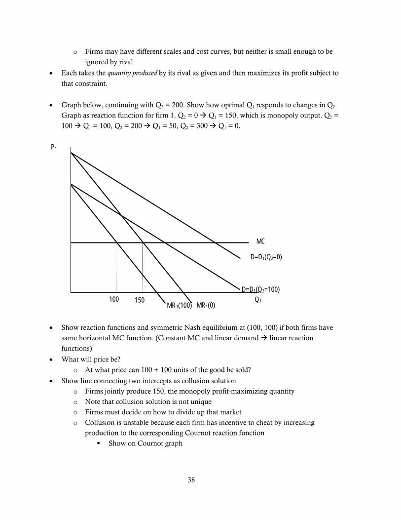
38
o Firms may have different scales and cost curves, but neither is small enough to be
ignored by rival
• Each takes the quantity produced by its rival as given and then maximizes its profit subject to
that constraint.
• Graph below, continuing with Q2 = 200. Show how optimal Q1 responds to changes in Q2.
Graph as reaction function for firm 1. Q2 = 0 Q1 = 150, which is monopoly output. Q2 =
100 Q1 = 100, Q2 = 200 Q1 = 50, Q2 = 300 Q1 = 0.
• Show reaction functions and symmetric Nash equilibrium at (100, 100) if both firms have
same horizontal MC function. (Constant MC and linear demand linear reaction
functions)
• What will price be?
o At what price can 100 + 100 units of the good be sold?
• Show line connecting two intercepts as collusion solution
o Firms jointly produce 150, the monopoly profit-maximizing quantity
o Note that collusion solution is not unique
o Firms must decide on how to divide up that market
o Collusion is unstable because each firm has incentive to cheat by increasing
production to the corresponding Cournot reaction function
Show on Cournot graph
P1
Q1
D=D1(Q2=0)
MC
MR1(0)
D=D1(Q2=100)
MR1(100) 100 150
39
Stackelberg industry leader model
• One dominant firm in the industry (ADM?); others are smaller
• Small firms will react to dominant one, but not vice versa
• Dominant firm can choose the point on the small firms’ reaction functions that maximizes
its profit and announce its decision
o It gets a “first-mover advantage” but (credibly) announcing its output decision and
that it won’t react to its rivals
Bertrand price-setting competition
• Cournot and Stackelberg models assume that firm chooses Q in response to rivals’ Q, and
that P is passively determined by quantity decisions
• What if firms strategize on P?
• With homogeneous good and constant and equal MC:
o Each firm’s optimal price is ε less than its rival’s, or MC, whichever is higher
o Reaction functions are parallel lines just above and below 45-degree line, but with
single intersection at MC value
o Result mimics competitive equilibrium: P = MC
• Can apply with differentiated products as well
o Each firm’s demand curve depends on own price and rival’s price
o Calculate profit-maximizing decision taking other price as given
40
Day 19: Game theory and oligopoly strategy
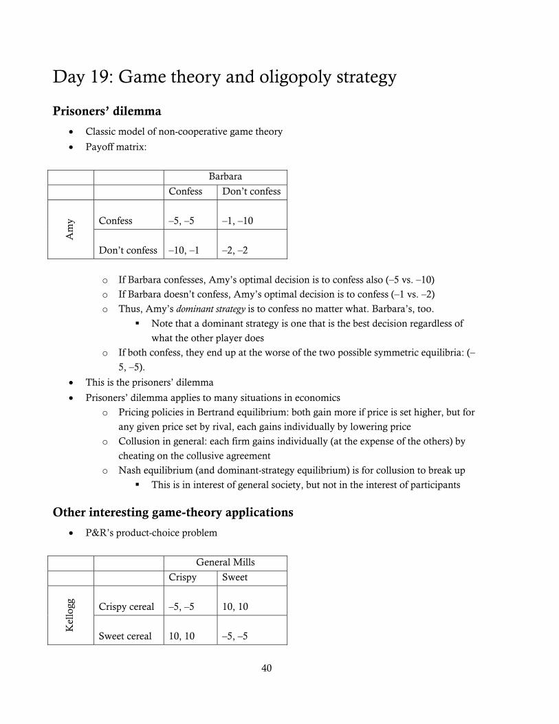
Prisoners’ dilemma
• Classic model of non-cooperative game theory
• Payoff matrix:
Barbara
Confess Don’t confess
Am
y
Confess
–5, –5
–1, –10
Don’t confess
–10, –1
–2, –2
o If Barbara confesses, Amy’s optimal decision is to confess also (–5 vs. –10)
o If Barbara doesn’t confess, Amy’s optimal decision is to confess (–1 vs. –2)
o Thus, Amy’s dominant strategy is to confess no matter what. Barbara’s, too.
Note that a dominant strategy is one that is the best decision regardless of
what the other player does
o If both confess, they end up at the worse of the two possible symmetric equilibria: (–
5, –5).
• This is the prisoners’ dilemma
• Prisoners’ dilemma applies to many situations in economics
o Pricing policies in Bertrand equilibrium: both gain more if price is set higher, but for
any given price set by rival, each gains individually by lowering price
o Collusion in general: each firm gains individually (at the expense of the others) by
cheating on the collusive agreement
o Nash equilibrium (and dominant-strategy equilibrium) is for collusion to break up
This is in interest of general society, but not in the interest of participants
Other interesting game-theory applications
• P&R’s product-choice problem
General Mills
Crispy Sweet
Kel
logg
Crispy cereal
–5, –5
10, 10
Sweet cereal
10, 10
–5, –5
41
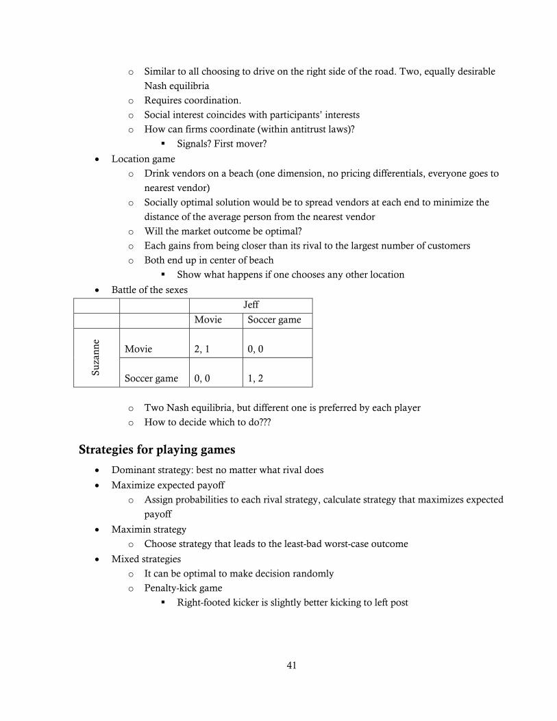
o Similar to all choosing to drive on the right side of the road. Two, equally desirable
Nash equilibria
o Requires coordination.
o Social interest coincides with participants’ interests
o How can firms coordinate (within antitrust laws)?
Signals? First mover?
• Location game
o Drink vendors on a beach (one dimension, no pricing differentials, everyone goes to
nearest vendor)
o Socially optimal solution would be to spread vendors at each end to minimize the
distance of the average person from the nearest vendor
o Will the market outcome be optimal?
o Each gains from being closer than its rival to the largest number of customers
o Both end up in center of beach
Show what happens if one chooses any other location
• Battle of the sexes
Jeff
Movie Soccer game
Suza
nne
Movie
2, 1
0, 0
Soccer game
0, 0
1, 2
o Two Nash equilibria, but different one is preferred by each player
o How to decide which to do???
Strategies for playing games
• Dominant strategy: best no matter what rival does
• Maximize expected payoff
o Assign probabilities to each rival strategy, calculate strategy that maximizes expected
payoff
• Maximin strategy
o Choose strategy that leads to the least-bad worst-case outcome
• Mixed strategies
o It can be optimal to make decision randomly
o Penalty-kick game
Right-footed kicker is slightly better kicking to left post
42
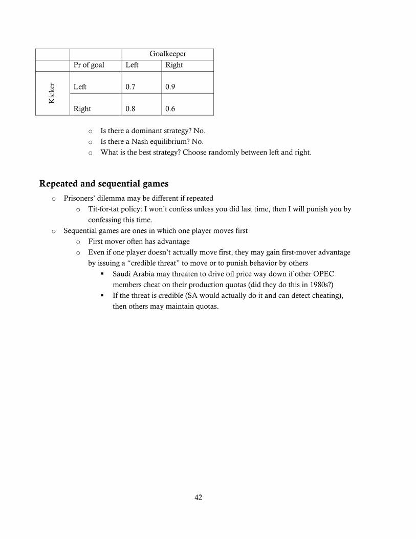
Goalkeeper
Pr of goal Left Right
Kic
ker
Left
0.7
0.9
Right
0.8
0.6
o Is there a dominant strategy? No.
o Is there a Nash equilibrium? No.
o What is the best strategy? Choose randomly between left and right.
Repeated and sequential games
o Prisoners’ dilemma may be different if repeated
o Tit-for-tat policy: I won’t confess unless you did last time, then I will punish you by
confessing this time.
o Sequential games are ones in which one player moves first
o First mover often has advantage
o Even if one player doesn’t actually move first, they may gain first-mover advantage
by issuing a “credible threat” to move or to punish behavior by others
Saudi Arabia may threaten to drive oil price way down if other OPEC
members cheat on their production quotas (did they do this in 1980s?)
If the threat is credible (SA would actually do it and can detect cheating),
then others may maintain quotas.
43
Day 20: Factor Markets
Factor markets are the “other side” of firms and households
• Firms as demanders of labor and capital resources
• Households as suppliers
Nature of factor demand
• “Derived demand”
o Demand for factors is based on the demand for the goods that they produce
o Factors that produce useless goods will not be in demand
Soccer players vs. horseshoe pitchers
Marginal revenue product
• Benefit to widget-producing firm of hiring one additional unit of labor = MRPL = MR × MPL
• R R QL Q L
Δ Δ Δ=
Δ Δ Δ
• If firm is competitive in output (widget) market, then MR = P and MRPL = P × MPL
o The latter is the value to society of using an additional unit of labor to produce
widgets
o The former is the value to the firm of using an additional unit of labor to produce
widgets
Profit maximization with one variable input
• Is firm is price-taker in labor market?
o Note that this is different question than being price-taker in output market
o Many firms that have monopoly power in output market have none in labor market
o Monopsony in the input market usually happens with highly specialized labor that is
used by only a few firms
• For price-taker: “Marginal factor cost” = “marginal expenditure” = w
o Hire the input (labor) until MRPL = w
o This means that MR × MPL = w or MR = w/MPL
o But w/MPL = MC if labor is the only variable input
o Thus, MRPL = w is the other side of the same coin as MR = MC.
• Firm’s demand curve for labor
o Equals MRPL curve if other inputs and product price are held constant
• Industry demand for labor:
o Not just horizontal summation of firm demands because each firm’s demand holds
product price constant
44
o It is reasonable to assume that product price will remain constant as any one firm
increases labor input (and thus output)
o It is not reasonable to assume that product price remains constant as all firms in the
industry increase labor input and output
o Show summation of individual firms’ labor demands
o Industry labor demand is less elastic because
As labor input of industry increases, production will increase and (demand
for product held constant) product price falls
Decline in product price reduces MR, which lowers each firm’s MRPL
This will shift the ΣMRPL curve to the left
Increase in industry labor demand is smaller than predicted by the
aggregation of firms’ labor demand curves
Long-run vs. short-run factor demand
• In long-run, firm can also switch among inputs
o This makes factor demand more elastic than in the short run
• Suppose that wage decreases:
o Initial shift down along MRPL(K=K0) curve to hire more labor
o More labor hired increases MPK and MRPK, which means more K is hired in long
run
o Increase in hiring of K increases MPL and MRPL, shifting curve to the right to
MRPL(K=K1)
o Demand is more elastic in long run when other factors can be varied
Economic rents
• We’ve encountered rents before: economic profits are rents, payments to specialized inputs
may be rents
• Economic rent is defined as payments to an input in excess of what would be required to
induce the input to be used
• The “producer-surplus triangle” in input markets constitute economic rents
• If input supply is perfectly inelastic (land), then all payments to input are rent
Monopsony in factor markets
• AEL = S and ME curves
• Profit maximization where MEL = MRPL
• Note that too little is hired, just as too little is produced by monopoly
• Firm that is both monopoly and monopsony will really hire too little labor because MRPL is
also “too low” because MR < P.
45
Monopoly union
• Upward-sloping SL indicates willingness to work given wage
• DL is demand for labor by firms
• Union will choose position on DL that maximizes workers’ rents
o MR curve lies below D as in output monopoly
o Set wage on D where MR = SL
o Rents are area above SL, below wage, and out to quantity hired (trapezoid)
46
Day 21: Labor Markets
Why labor markets differ from other markets
• Labor suppliers care about the circumstances of their employment (unlike capital, energy, or
material inputs and unlike consumer goods)
o Some jobs have more disutility than others based on working conditions, co-workers,
etc.
• Labor has many alternative reservation uses (leisure)
• Labor is far more heterogeneous than any other good or service
o Differences in location, skills, preferences, etc.
Basics of labor supply
• Show goods/leisure tradeoff (as in problem set)
• Describe income and substitution effects of wage increase
o Substitution effect: Wage increase raises the opportunity cost of leisure in terms of
goods: goods are now a cheaper source of utility relative to leisure
Work more (less leisure) and consume more
o Income/wealth effect: Wage increase makes one wealthier (assuming one works)
and thus pushes the budget constraint out
Work less (more leisure, assuming leisure is normal good) and consume
more
o If income effect dominates, then labor supply curve will bend backward
Plausible for permanent, but not temporary, wage changes
Perhaps more plausible at higher levels of wages
• Why do so many people work 40 hours/week?
o Discontinuity of hours opportunities on demand side
o Workers must often conform to common work schedule
Shift work
Work during business hours
o Forces large groups of workers to work the same number of hours
Social conventions dictate how the workweek is divided up
Differs across countries and times
8 hour day is convenient because it allows 3 shifts
Human capital
• Acquired characteristics that increase productivity of individual workers
o Education
o Experience-based skill acquisition (formal or informal)
o Health
47
• Differences in human capital lead to segmentation of labor market
o Workers in different segments do not compete directly against each other
o In long run, workers can acquire human capital and move between market segments
Unions
• Collective bargaining
o Act as a monopoly seller of labor to unionized firm or industry
o Chooses point on firm’s (or industry’s) labor demand curve
o Faces tradeoff between higher wages and higher employment similar to tradeoff
faced by monopoly firm
o Not clear what objective would be appropriate for union
Revenue maximization?
How to balance getting the best wage deal for current members vs. expanding
employment and gaining new members?
Are there asymmetries between the interests of existing members (who might
lose jobs if wages were increased more) and potential members (who might
gain jobs if wages were increased less)?
• Management of labor relations
o Proponents of unions often stress unions’ potential role for increasing productivity by
providing an institutional mechanism for grievances, layoffs, firing rules, etc.
• How do unions affect employment?
o Lower it through attempts to raise wages
o Raise it through positive effects on labor productivity
Wage differentials
• Demand-side differentials
o Different categories of workers (or even different workers) have different MPs.
o Those that are more productive are more valuable to employers and receive higher
wages
• Supply-side differentials
o Work that is less desirable should pay a compensating wage differential to induce
workers to do it
o Dangerous and unpleasant jobs should have higher equilibrium wages
• Mobility as equilibrating force
o Are workers and employers sufficiently informed and mobile to move when wages
are misaligned?
48
Motivating workers
• If working hard is less pleasant than shirking, then workers will want to shirk and get paid
rather than working hard
o This is bad for employer, who gets less output
o Can employer detect shirking and fire those who shirk? Maybe, but maybe not
• Piece-rate pay
o If output of individual worker can be identified, then workers can be paid on the
basis of individual productivity and won’t have incentive to shirk
Commissions
Lawyers
Financial traders rewarded based on portfolio performance
Piece-rate agricultural work
o What about quality? Can employer measure the quality as well as the quantity of
worker’s output?
• Efficiency wages
o Pay wage above the equilibrium, fire anyone caught shirking
o Workers may work hard even if probability of detection is low in order to avoid
being fired and losing higher wage
• Stock ownership, profit-sharing, profit-based bonuses, options
o Giving individual workers an interest in profits of firm
o Ownership is sufficiently dilute that if may not be very effective
o Can lead to short-term stock-price maximization rather than long-term profit
maximization
Especially if shares can be sold soon or options expire soon
Minimum-wage laws
• Standard analysis: price floor may prevent market from clearing
o Lowers employment and leads to excess supply of labor: unemployment
• Minimum wage is much lower than average wage, even in Oregon
o May be higher than equilibrium wage for some segments of labor market
o Some evidence (conflicting) that minimum wage raises unemployment among low-
skill workers
• Non-clearing labor market allows for discrimination by employers about which of the
available excess supply of workers to hire
o Would tend to hire those with more experience
o Can be hard on teens and minorities
49
Day 22: Capital Markets
Definitions
• Key characteristic of capital: durability
o Economic value of “time” is an essential element of capital theory
o How much is it worth to use a particular durable good for a period of time?
• Stocks vs. flows
o Profit, expenditures, revenue, cost, consumption are all flows
o Capital, wealth, assets, debts are all stocks
o Key stocks and flows in capital theory
Capital stock is amount of capital at a moment in time
Gross investment is flow of new capital entering the stock
Depreciation is flow of lost value of K due to aging, obsolescence, etc.
Net investment = ΔK = gross investment – depreciation
Rate of return and present value
• Let R be the (nominal) market interest rate per year
o 0.05 = 5%
• $1.00 this year yields $(1 + R) one year from now, or $(1 + R)2 two years from now (if the
interest rate is constant), or $(1 + R)n n years from now.
o Note that n need not be an integer and need not be positive
• ( )1n
FV PV R= × + gives future value in terms of present value
• ( )1
n
FVPV
R=
+ gives present value in terms of future value
o This is crucially important formula in economics and finance
o It tells the value today of a payment to be made in the future
Bond prices
• Bond is a promise to pay specified amounts on specified dates
• Typical “coupon” bond has face value F and coupon interest rate c (which may or may not
equal current market interest rate R) and maturity n years
o Annual coupon payments are cF for each of the next n years
o Principal is repaid n years in the future
o (Ignoring risk) the price of bond must equal the present discounted value of these
payments
o ( ) ( ) ( )2 ...
1 1 1 1n n
cF cF cF FPDV
R R R R= + + + +
+ + + +
50
• For “consol” or “perpetuity” that is never repaid, n → ∞, so
( )2 ...1 1
cF cF cFPDV
R RR= + + =
+ +
Calculating the rate of return or effective yield on a capital investment
• We can use the PDV formula either to calculate the equilibrium price of a bond, given F, c,
and R or to calculate the “rate of return” on an investment if we know:
o The current cost of the investment project and
o The future returns on the investment project
• ( )1
tK t
t
MRPKNPV P
R= − +
+∑ where PK is the current price paid for the capital good and MRPKt
is the marginal revenue product of the capital good t periods into the future.
o The capital investment project is beneficial to the firm if NPV > 0.
o We can show under reasonable assumptions that NPV > 0 iff MRPK > PK (R + δ), so
this motivates the “user cost of capital” that we studied in production theory
Real vs. nominal interest rates and returns
• Inflation affects the purchasing power of dollar over time
o Purchasing power is what matters to people, so we must account for inflation in
measuring returns to bonds, capital, etc.
• Suppose that inflation rate is π and nominal interest rate is R
o 1t t
t
P PP
+ −π = , so 1 ,t t tP P P+ − = π and ( )1 1t tP P+ = + π or 1 1t
t
PP+ = + π
Example: if current widget price is $100 and inflation is 0.04, then widget
price next year is $104
o Lend 1 widget worth of money this year: how many widgets worth will you get back
next year?
One widget = $Pt now
You get back $Pt (1 + R) next year
Each dollar next year buys 1/Pt + 1 widgets, so you get back
( )1
11
1t
t
P RR
P +
++ =
+ π widgets next year.
Your real interest rate (in terms of purchasing power) is 1
11
Rr
++ =
+ π, which
is approximately r R= − π
51
Loanable-funds market and interest-rate determination
• In the long run (and perhaps in the short run), the interest rate is determined by the flows of
lending (saving) and borrowing (for investment)
o Both saving and investment depend on the real cost of borrowing r, not on the
nominal rate R
• Supply of saving is probably upward-sloping in the real interest rate
• Demand for investment/borrowing should be downward-sloping in the real interest rate
• Equilibrium in the flow of loanable funds determines real interest rate
Structure of interest rates by term and risk
• In practice, the real return on an asset is rarely known with certainty in advance
o U.S. inflation-adjusted bonds?
o Inflation risk on standard Treasure bonds/bills
o Default risk on most private bonds and loans
• Variable returns that are unknown when the loan is made (or asset is bought) = risk
• If savers/lenders are generally risk averse, then they will demand a higher real interest rate
on assets that add to the riskiness of their portfolios
o Note that some assets with variable returns can insure against others if their returns
are negatively correlated
• Risky assets will have to have higher expected rates of return in order to compensate for risk
• Interest rates and rates of return may also vary with other characteristics
o Term to maturity
o Liquidity
52
Day 23: General Equilibrium
Nature of general-equilibrium analysis
• Most of what we have done this semester has been partial equilibrium—looking at one market
at a time
• Markets interact through many channels
o Changes in output markets affect demand curves for inputs through MR MRP
o Changes in factor markets affect supply curves for outputs through w MC
o Changes in goods markets affect demand for substitutes and complements
o Changes in factor markets affect incomes, which affects demand for goods
o Changes in one factor market affect the demand for other factors that are substitutes
or complements
• Changes in preferences or technology set of a whole chain of reactions through various
markets
o Evaluating the final effect of any kind of change requires thinking through the
general equilibrium response, not just a partial equilibrium analysis
• We can’t do justice to general equilibrium with two-dimensional diagrams, but multivariate
mathematical methods can solve these models easily
Concepts of efficiency in general equilibrium
• General concept of Pareto efficiency
o No one can be made better off without making someone else worse off
o There are no unexploited gains: no way to make everyone better off
o Not unique: alternative Pareto efficient equilibria in which
I am rich and you are poor
You are rich and I am poor
o Pareto criterion is actually rather weak one
• Efficiency in exchange
o There is no way to reallocate goods across consumers that will improve utility of one
without reducing utility of another (or improve utility of both)
o 1 2AB ABMRS MRS= , where A and B are goods, 1 and 2 are consumers
• Efficiency in input use
o There is no way to reallocate labor and capital across industries to allow one to
produce more without the other producing less (or increase production of both)
o A BLK LKMRTS MRTS=
• Allocative (output) efficiency
o There is no way to reallocate labor and capital across industries to allow one person
to get more utility without someone getting less
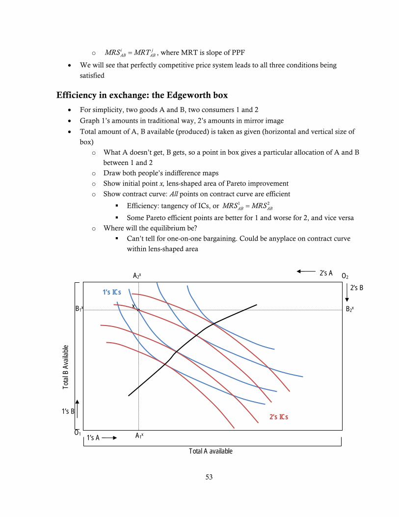
53
o i jAB ABMRS MRT= , where MRT is slope of PPF
• We will see that perfectly competitive price system leads to all three conditions being
satisfied
Efficiency in exchange: the Edgeworth box
• For simplicity, two goods A and B, two consumers 1 and 2
• Graph 1’s amounts in traditional way, 2’s amounts in mirror image
• Total amount of A, B available (produced) is taken as given (horizontal and vertical size of
box)
o What A doesn’t get, B gets, so a point in box gives a particular allocation of A and B
between 1 and 2
o Draw both people’s indifference maps
o Show initial point x, lens-shaped area of Pareto improvement
o Show contract curve: All points on contract curve are efficient
Efficiency: tangency of ICs, or 1 2AB ABMRS MRS=
Some Pareto efficient points are better for 1 and worse for 2, and vice versa
o Where will the equilibrium be?
Can’t tell for one-on-one bargaining. Could be anyplace on contract curve
within lens-shaped area
1’s B
1’s A
2’s B
2’s A
Total A available
O1
O2
Total
B A
vaila
ble
x B2x
A2x
B1x
A1x
1’s ICs
2’s ICs
54
• Efficiency of perfect competition
o In competitive equilibrium, each consumer sets 1 2AAB AB
B
PMRS MRS
P= = , so they are
equal to each other and competitive equilibrium has efficiency of exchange
o This is the first theorem of welfare economics
• Equality vs. efficiency: Any point on contract curve is efficient (wrt exchange), some are
more equitable than others
o By varying the initial endowment of goods, any point on the contract curve can be
achieved as a competitive equilibrium, so efficiency and equality are not in conflict
o This is the second theorem of welfare economics
Efficiency in input use
• Same basic idea:
o Total labor and capital in Edgeworth box; allocation between two firms (or
industries) A and B
o Production contract curve: Efficient outcome is where isoquants are tangent to one
another
Different points on contract curve correspond to different points on the PPF
Some have high output of A, others high output of B
All allocate resources efficiently given the amounts of A and B produced
At all efficient points: A BLK LKMRTS MTRS=
• Competitive equilibrium is efficient in input use because each firm equates
A BLK LK
wMRTS MTRS
r= =
Allocative (output) efficiency
• Which point on PPF to choose?
• Absolute slope of PPF is MRTAB = MCA/MCB
• Efficiency requires that iAB ABMRT MRS= for all consumers i
• Competitive equilibrium achieves this condition since MC = P for all goods, so
iA AAB AB
B B
MC PMRT MRS
MC P= = =
International trade and the PPF
• If a country can trade freely at international prices, then it can consume along line tangent to
PPF with slope = world price ratio.
55
Day 24: Economics of Information
Information problems
• So far, we have assumed that buyers and sellers are perfectly informed about the two things
that matter:
o Price
o Quality characteristics of product
• In many markets, traders have asymmetric information: One party (buyer or seller) has
information that the other does not have
• Asymmetric information can lead to several kinds of problem
o Adverse selection
o Moral hazard
o Principal-agent problems in general
Adverse selection
• Adverse selection occurs before transactions occur.
• Two kinds of agents on one side of market: good and bad
• Good agents cannot credibly convince transaction partners that they are good
• Only bad agents enter the market because good agents don’t find it optimal to transact when
partner assumes they are bad
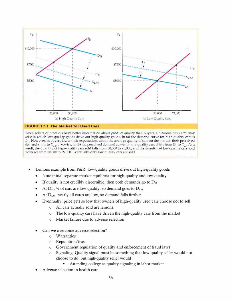
56
• Lemons example from P&R: low-quality goods drive out high-quality goods
• Note initial separate-market equilibria for high-quality and low-quality
• If quality is not credibly discernible, then both demands go to DM
• At DM, ¾ of cars are low-quality, so demand goes to DLM
• At DLM, nearly all cares are low, so demand falls further
• Eventually, price gets so low that owners of high-quality used cars choose not to sell.
o All cars actually sold are lemons.
o The low-quality cars have driven the high-quality cars from the market
o Market failure due to adverse selection
• Can we overcome adverse selection?
o Warranties o Reputation/trust o Government regulation of quality and enforcement of fraud laws o Signaling: Quality signal must be something that low-quality seller would not
choose to do, but high-quality seller would Attending college as quality signaling in labor market
• Adverse selection in health care
57
o Can insurance companies charge higher premiums to people with high probability of illness? (Should they?)
o If they cannot, healthy people may not sign up for insurance. o Only sickly people will insure, and insurance costs will be very high. o Obama policy prohibits cutting off insurance to people with pre-existing
conditions and terminating policies when someone gets really sick. Good policies for other reasons, but increases adverse selection
o Obama policy requires everyone to sign up for insurance An attempt to get around the adverse selection problem by keeping the
healthy people in the pool
Moral hazard
• Unlike adverse selection, moral hazard occurs after a contract is signed
o One party changes behavior in a way that harms the other, but cannot be detected
because of asymmetric information
• Most common in insurance markets, but happens elsewhere too
o If you are insured against a loss, you may take less precaution to avoid it
o If insurance company does not have complete information about your behavior, so it
can’t prevent this behavior with clause in contract
They try to discourage moral-hazard behavior with incentives:
• Experience-rated premiums that go up when you have a claim
• Background checks that examine your prior behavior (including
credit ratings?)
• Moral hazard in health care
o If the insurance company is paying, then both you and your doctor have incentive to
order more tests, more procedures of low value, etc.
Principal/agent problems
• Principal hires agent to work to accomplish principal’s goals
o Shareholders hiring managers to maximize profit
o Managers hiring workers to produce output
o Customers hiring service worker to produce almost anything (fix car, paint house,
etc.)
• Principal cannot perfectly monitor agent’s behavior, so asymmetric information
o Agent has incentive to pursue own alternative objectives rather than those of the
principal
o Principal must either invest in better monitoring or employ incentive contracts to
align incentives
Efficiency wage, merit pay, bonuses
Profit-sharing, ESOP, or stock options
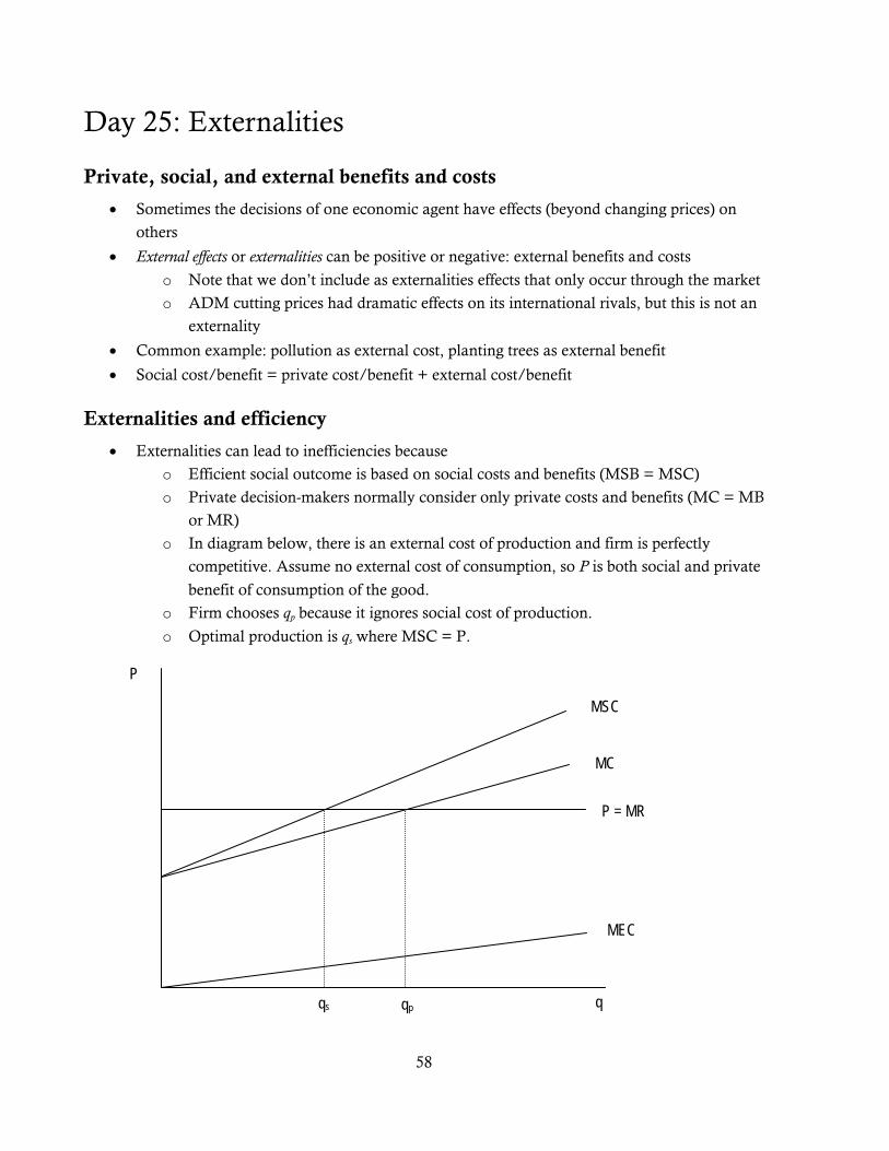
58
Day 25: Externalities
Private, social, and external benefits and costs
• Sometimes the decisions of one economic agent have effects (beyond changing prices) on
others
• External effects or externalities can be positive or negative: external benefits and costs
o Note that we don’t include as externalities effects that only occur through the market
o ADM cutting prices had dramatic effects on its international rivals, but this is not an
externality
• Common example: pollution as external cost, planting trees as external benefit
• Social cost/benefit = private cost/benefit + external cost/benefit
Externalities and efficiency
• Externalities can lead to inefficiencies because
o Efficient social outcome is based on social costs and benefits (MSB = MSC)
o Private decision-makers normally consider only private costs and benefits (MC = MB
or MR)
o In diagram below, there is an external cost of production and firm is perfectly
competitive. Assume no external cost of consumption, so P is both social and private
benefit of consumption of the good.
o Firm chooses qp because it ignores social cost of production.
o Optimal production is qs where MSC = P.
P
q
P = MR
MEC
MC
MSC
qs qp
59
• For industry as a whole, supply curve is aggregation of MC curves, but social optimum
would be aggregation of MSC curves.
o Note deadweight loss triangle associated with overproduction
o Interpret vertical distances as excess of marginal social cost over benefit
• External effects in consumption lead to overuse (if costs) or underuse (if benefits)
Optimal amount of pollution
• Marginal social cost of pollution
o Probably upward sloping in amount of emissions ($/unit of emissions on vertical
axis)
o No one notices a little pollution but once it becomes a problem the marginal cost
increases
• Marginal cost of abatement
o Abatement is not free
It uses economically valuable resources or
It involves forgoing the production of economically useful goods
o Social cost of reducing pollution is high when there is much abatement (emissions
are low) and low when we are only abating the easily avoidable emissions
• Optimal amount of pollution:
o Where MCA = MSC = pE, E = E*
Policy alternatives to achieve optimal pollution
• Emission standards
o Set maximum emission allowed at E*
o Works OK if all firms have similar MCA, so that E* can easily be allocated based on
output or other criteria: can only emit a certain amount per unit of output so that
total adds up to E*
• Pollution fees
o Set fee at pE per unit of emissions
o This will “internalize” externality and make firm’s MC = MSC because tax = MEC
o This works OK with different MCA across firms because each will make individual
decision about pollution based on internalized costs
• “Cap and trade” system of transferable emission permits
o Need permit to emit pollutant
o Issue E* amount of permits to assure that total pollution is optimal
o Allow firms to exchange permits to assure “efficiency of exchange”
o Those with highest MCA will be willing to pay most for permits and will buy them
o Those will lowest MCA will abate on their own and sell their permits
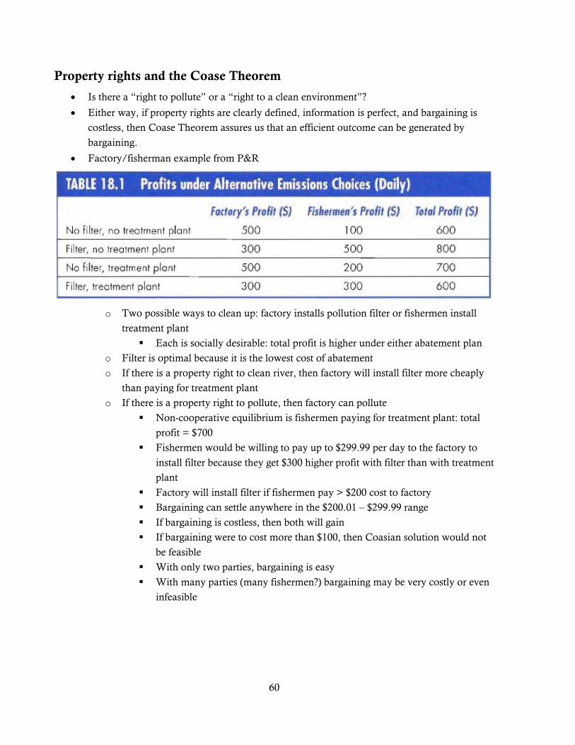
60
Property rights and the Coase Theorem
• Is there a “right to pollute” or a “right to a clean environment”?
• Either way, if property rights are clearly defined, information is perfect, and bargaining is
costless, then Coase Theorem assures us that an efficient outcome can be generated by
bargaining.
• Factory/fisherman example from P&R
o Two possible ways to clean up: factory installs pollution filter or fishermen install
treatment plant
Each is socially desirable: total profit is higher under either abatement plan
o Filter is optimal because it is the lowest cost of abatement
o If there is a property right to clean river, then factory will install filter more cheaply
than paying for treatment plant
o If there is a property right to pollute, then factory can pollute
Non-cooperative equilibrium is fishermen paying for treatment plant: total
profit = $700
Fishermen would be willing to pay up to $299.99 per day to the factory to
install filter because they get $300 higher profit with filter than with treatment
plant
Factory will install filter if fishermen pay > $200 cost to factory
Bargaining can settle anywhere in the $200.01 – $299.99 range
If bargaining is costless, then both will gain
If bargaining were to cost more than $100, then Coasian solution would not
be feasible
With only two parties, bargaining is easy
With many parties (many fishermen?) bargaining may be very costly or even
infeasible
61
Tragedy of the commons
• Common-property resources such as fish in the sea, oil wells tapping common underground
pool, Commons dishes
• All have free access: MC for individual is zero, MC for group is positive
o Or private MC < MSC if we consider non-depletion costs of fishing > 0
• Each individual’s consumption has social cost but no private cost
• As with other MEC > 0 situations, overconsumption will result
• M&M experiment?
62
Day 26: Public Goods
Voluntary contribution experiment
• Distribute materials and run experiment
• Discussion
o Individually optimal behavior
Return to private project
Individual and collective return to public project
o Collectively optimal behavior
o Can we rely on voluntary contributions to produce desirable public goods?
Why is Reed experiment different from real-world applications?
Easier or harder? What factors make it easy or hard to collect contributions?
Public goods
• Two essential characteristics: nonrivalry and nonexcludability
o Can be more or less nonrivalry and nonexcludability: not necessarily perfect
• Nonrivalry: consumption by one does not diminish the ability of others to consume
o Cinnamon rolls vs. cinnamon roll recipe
• Nonexcludability: not feasible to restrict consumption of good to those who pay
o Small park vs. large park
• Everyone should and will have access to the amount of the public good provided
o MC of extending availability to additional person is zero, so no one should be
restricted from using
o Impossible to exclude anyway
• If everyone can use without paying, then all have incentive to be free riders and not pay
• If everyone is a free rider, then no one pays and there is no revenue from producing the good
• Therefore, public goods will usually be underprovided by the market
o Role for government provision out of tax revenue
o Pose question from experiment: would everyone have voted for a “tax” to require all
participants in the experiment to contribute fully to the public project?
o Each votes “yes” because they are committing themselves only contingent on
committing everyone else
Everyone still has an incentive to cheat on their taxes once the law is passed,
though…
• What goods are public goods?
o National defense
o Broadcast radio & TV
o Street lights
o Information on new product?
63
Optimal quantity of public goods
• Since same unit can be consumed by all consumers, we add demand curves vertically
o Sum the willingness to pay of all consumers in order to get the total value of all
consumers for that unit of the good
• Optimal level of provision is where vertically aggregated demand curve intersects MC
64
Day 27: Income Distribution and Poverty
What concept of equality/equity is appropriate?
• Equality of outcome vs. equality of opportunity
o Some may choose to work less or not to invest in human capital. Should they earn
equal incomes?
• Rawlsian justice principal
o Choose income distribution as if you did not know your position in it
Facts about the distribution of income, wealth, and earnings
• Lorenz curve
o % of (income, earnings, wealth) received by bottom n% of population
o How curves for income, earnings, wealth
o Why is wealth so much more skewed than others?
Age and accumulation
o Earnings more skewed than income because of transfer payments
• Gini coefficient
o Area above Lorenz curve divided by total area under equality line
• Cross-section data
• Time-series data
What determines the income distribution?
• Marginal-productivity theory of income distribution
o Quantity of resources owned
How are they acquired? Inherited, saved/invested?
o Value of these resources
Marginal product
Scarcity/available substitutes
Foresight and luck in choosing resources that will be scarce
o Choice of market use of resources vs. reservation use
• Okun’s determinants
o Acquired assets
o Natural abilities
o Effort
o Related supplies and demands
• Others
o Compensation for risk (labor or capital)
o Luck
65
o Others?
Equality vs. efficiency
• Welfare theorems and distinction between initial wealth and outcome wealth
• Why does greater equality mean less efficiency?
o Possibility of increased reward motivates individual actions:
Production
Investment in human and physical capital
o Leaky bucket: how much of a leak is OK
Normative question
How leaky is the bucket?
Does leakiness vary over time and countries?
• Government programs to promote equality
o Explicit transfers
Social Security, welfare, other transfer programs
o Progressive taxation
Rich pay a higher share of their income in income taxes
o Public education
Provide basic human capital to all (not totally successful in achieving
equality here)
o Others?
66
Day 28: Second Mid-Term Exam
Day 29: Intro to Macroeconomics
Macro vs. micro
• Complementary views of the economy
• Micro studies behavior of individual households, firms, and industries
• Macro studies the relationships among aggregate economic variables such as income, the
general price level, and the aggregate levels of employment and unemployment
Variables of macroeconomics
• Gross domestic product (or GNP) measures income and output at the aggregate level
• General price level/inflation rate
o Note distinction between relative prices and the general price level
• Employment and unemployment rates
• Interest rates, exchange rates, trade balance, etc.
Models
• A model is a simple representation of a complex system, designed to illustrate in an easily
understood way some basic properties of the system that are not easily seen due to its
complexity
o Globe as a model of the earth
o Every model simplifies away much of the complexity
Choose what to ignore and what to emphasize about system
Cannot answer questions about what you have simplified away!
• Categories of variables: exogenous, endogenous, (predetermined)
• Models are built of equations describing connections among the variables
o Structure of model: assumptions about behavior of people and markets
o Output of model: conclusions about how exogenous variables affect endogenous
variables
• Different assumptions lead to different conclusions
o Market-clearing assumption vs. wage/price stickiness
• Approaches to modeling (Mankiw article)
o Engineering approach: top-down, looking at and explaining correlations among
aggregate variables
o Scientific approach: bottom-up, looking at behavior of individuals and building up
the model from microfoundations
o Neither is better; they can be complementary
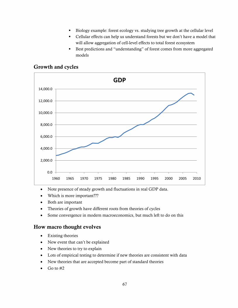
67
Biology example: forest ecology vs. studying tree growth at the cellular level
Cellular effects can help us understand forests but we don’t have a model that
will allow aggregation of cell-level effects to total forest ecosystem
Best predictions and “understanding” of forest comes from more aggregated
models
Growth and cycles
• Note presence of steady growth and fluctuations in real GDP data.
• Which is more important???
• Both are important
• Theories of growth have different roots from theories of cycles
• Some convergence in modern macroeconomics, but much left to do on this
How macro thought evolves
• Existing theories
• New event that can’t be explained
• New theories to try to explain
• Lots of empirical testing to determine if new theories are consistent with data
• New theories that are accepted become part of standard theories
• Go to #2
0.0
2,000.0
4,000.0
6,000.0
8,000.0
10,000.0
12,000.0
14,000.0
1960 1965 1970 1975 1980 1985 1990 1995 2000 2005 2010
GDP
68
Macroeconomic traditions: fluctuations
• Classical macroeconomics (before 1935)
o Basic micro general-equilibrium theory (bottom up)
o Only things missing are general price level and role for money
o Quantity theory: MV = PY
o Inflation = money growth – real-output growth
o Money supply has no effect on real variables
o No explanation for unemployment or business cycles
• Keynes and Keynesians (1935–1975)
o Great Depression: resources underutilized
Not in general equilibrium
o General Theory as original text of macroeconomics
o Stressed non-market clearing, but no micro foundations in his model
o Shortfall in “aggregate demand”
Monetary policy can affect aggregate demand, so it might be able to help
Fiscal policy can affect aggregate demand as well (and Keynes emphasized)
• Neoclassical (1975–present)
o Re-assertion of importance of microfoundations
o Linkage of long run to short run: model is more classical in long run, more
Keynesian in short run
o Highlighted crucial role of expectations
o Evolved into and out of RBC models
o Development of DSGE models
• New Keynesian (1980–present)
o Accepted challenge of microfoundations from neoclassical, but applied methods to
models with price/wage stickiness and no market clearing
o Rational reasons why markets might not clear in the short run
Macroeconomic traditions: growth
• Neoclassical Solow growth model
o Dynamic classical model
o Population growth and technological progress are exogenous
o Slowdown in productivity growth from 1973–95: Why?
• Endogenous growth models
o Examine micro underpinnings of R&D, human capital, and technological progress
o Try to model technological progress in general equilibrium with growing economy
69
Day 30: Measurement in Macro • Macro is an empirical discipline: built to explain movements in variables.
o Observable variables are key constraint; they define the space within which
macroeconomists work.
• Three key categories of variables we will consider
o National income/output
o Price level
o Employment and unemployment
• All three of these are key endogenous variables that in some way or another are thought to
be important for social welfare, which can’t be measured directly (case study)
National income and product accounts
• Circular flow (diagram)
• Income = Expenditures = Output
• Breakdowns of each
o Income = Wages & salaries + Interest + Rent + Proprietors’ income + Corporate
profit + Small categories (indirect taxes in here, too)
o Expenditures = Consumption + Investment + Government spending + Net exports
o Output = Value added in different industries
• Measuring the flow: How can we add up all the goods and services produced?
o Must use dollars
o Better than weight, etc.
• GDP = market value of all final goods and services produced in an economy in a given
period of time.
o GDP is a flow measured at annual rate (measured over period of time)
o Market value = what someone was willing to pay
Includes excise/sales taxes
o Final vs. intermediate
Intermediate is not durable; capital is
o In an economy
GDP = produced within U.S.
GNP = produced by U.S. residents
Very close for U.S., not for some other countries (Luxembourg)
• What’s left out of GDP?
o Leisure
o Nonmarket production
o Underground economy
• Real vs. nominal GDP
o Discuss price indexes later
70
o Real GDP is usually more important
• Is more real GDP better?
Measuring aggregate prices
• Major indexes
o CPI (from BLS)
o GDP deflator (or chain-weighted price index)
o PCE and core PCE index from GDP accounts (used by Fed)
• Methods
o Laspeyres index (CPI)
, ,
1
, ,1
100
N
i t i bi
t N
i b i bi
P QP
P Q
=
=
= ×∑
∑
o Paasche index (GDP deflator)
, ,
1
, ,1
100
N
i t i ti
t N
i b i ti
P QP
P Q
=
=
= ×∑
∑
o Chain-weighted index (now preferred GDP price index)
, ,
1
1, 1 ,
1
N
i t i tt i
Nt
i t i ti
P QP
P P Q
=
−−
=
=∑
∑ and build up series as a chain from base year = 100
• Biases
o CPI overstates and deflator understates inflation due to substitution bias
o Both overstate inflation due to entry of new goods
o Both overstate inflation if there are improvements in quality that are not accounted
for
o Outlet substitution is CPI problem
• CPI tells us that prices are 19 times higher than in 1913.
o Which would you rather have: $1900 to spend now or $100 to spend from the 1913
Sears catalog?
• Optimal inflation rate?
o Boskin Commission argues that CPI overstates inflation by 0.75–1.50 percentage points
per year
o Fed has “comfort range” for inflation (core PCE) of 1.5 – 2%
Labor data
• Working-age population = Labor force + Not in labor force
71
• Labor force = Employed + Unemployed
• CPS and the relevant questions
o Did you work during reference week? (Yes = employed)
o If not, were you actively seeking work or awaiting recall from layoff? (Yes =
unemployed, No = not in LF)
o Borderline cases: discouraged workers, underemployed workers, high-reservation-
wage workers (CPS now collects data on first two)
o Long-term vs. short-term unemployed (why is this a concern?)
• Unemployment rate = # Unemployed / Labor force
o Note that discouraged workers are left out of both numerator and denominator
• Unemployment = search
o Matching theory: Unemployed workers and vacant jobs coexist, awaiting match
o Matching may work better in some times and places than in others
o Incentives to continue search vs. accept job (unemployment benefits)
• Natural and optimal unemployment rates
o Optimal rate is not zero due to benefits of search
o Natural rate is not zero, but may be larger than optimal rate due to distorted
incentives encouraging search
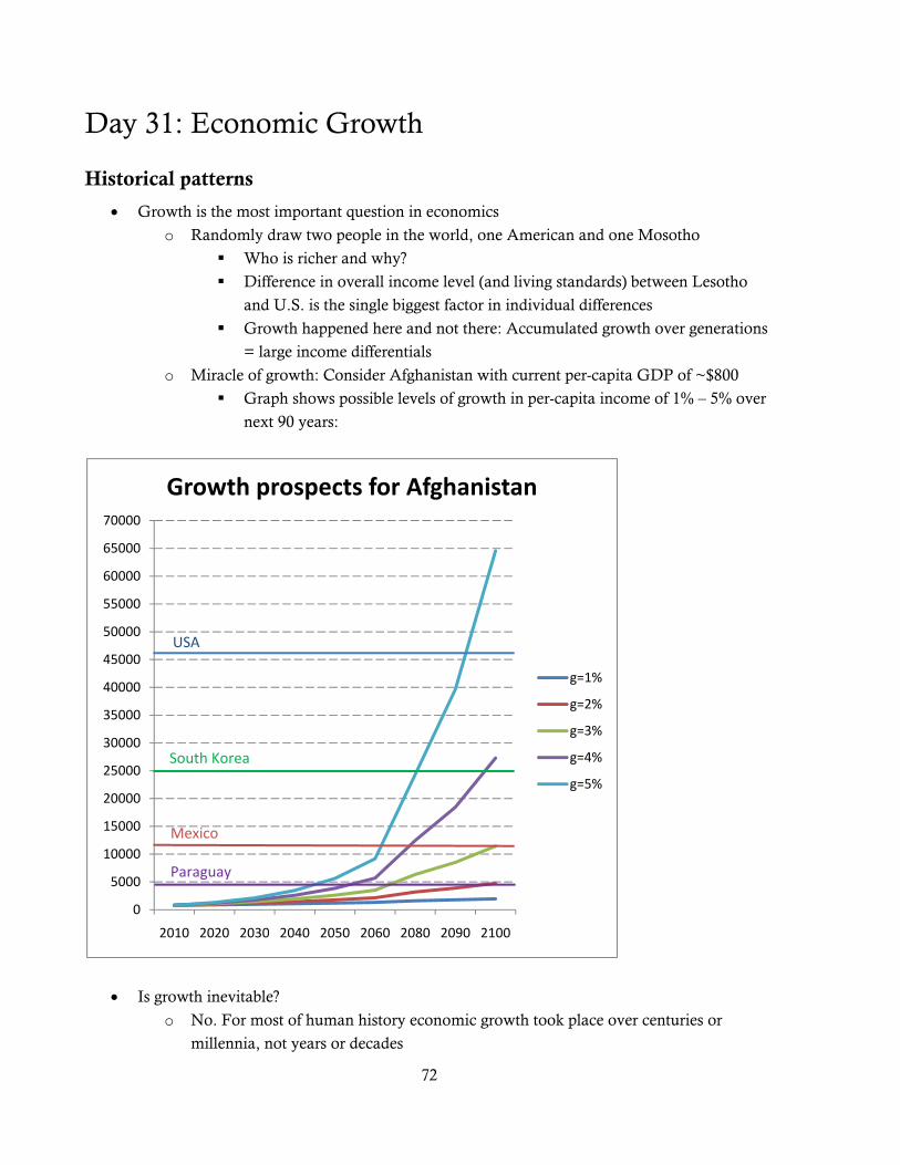
72
Day 31: Economic Growth
Historical patterns
• Growth is the most important question in economics
o Randomly draw two people in the world, one American and one Mosotho
Who is richer and why?
Difference in overall income level (and living standards) between Lesotho
and U.S. is the single biggest factor in individual differences
Growth happened here and not there: Accumulated growth over generations
= large income differentials
o Miracle of growth: Consider Afghanistan with current per-capita GDP of ~$800
Graph shows possible levels of growth in per-capita income of 1% – 5% over
next 90 years:
• Is growth inevitable?
o No. For most of human history economic growth took place over centuries or
millennia, not years or decades
0
5000
10000
15000
20000
25000
30000
35000
40000
45000
50000
55000
60000
65000
70000
2010 2020 2030 2040 2050 2060 2080 2090 2100
Growth prospects for Afghanistan
g=1%
g=2%
g=3%
g=4%
g=5%
USA
Mexico
South Korea
Paraguay
73
o Only since the Industrial Revolution in England around 1800 has growth been
consistently positive and at a rate where each generation was noticeably better off
than its predecessor.
o Even this growth has not been shared by all parts of the world.
• Patterns of U.S. growth
o We have reliable data only back to about 1950 for most countries (later for some)
Fragmentary data for earlier periods allow partial reconstruction of GDP, but
these numbers are probably much less reliable
o As per case study: U.S. (and other countries) grew rapidly from 1950–73, then slowly
after that.
It’s difficult to measure growth in capacity output over short periods due to
business cycles disrupting the trend
o Some evidence of a resurgence in growth after 1995, but only short period of data.
Sources of growth
• Aggregate production function: ( ), ,Y F K L A=
o This represents productive capacity if K is available capital, L is labor force.
• Capacity GDP grows if there is growth in K, L, or A.
o Mention growth accounting from case study
• CRTS Y/L will grow with growth in K, A.
Theories of growth
• Neoclassical growth model (Solow)
o Can Y/L continue to grow indefinitely due solely to “capital deepening”?
Not if there are diminishing marginal returns to K
Eventually, as K/L increases, MPK declines and gain to Y/L from increasing
K/L gets tiny
If technology is fixed, then economy reaches a steady-state with constant per-
capita income
o Only technological progress can sustain increasing per-capita income over the long
run
Rate of productivity growth = growth rate of per-capita income in steady
state
Solow model takes technological progress to be exogenous
Show steady-state growth path and convergence to it
(Only) Long-run policies aimed at increasing technological progress may be
successful in increasing growth.
o Convergence
74
If two economies are similar (saving rates, access to technology, population
growth, etc.) then over time they will converge to the same steady-state
growth path: same per-capita income
Countries that start with lower K/L will converge upward to path.
Example of East and West Germany
How long will convergence take?
• Evidence suggests that the half-life of the gap is 18–50 years.
• Endogenous growth theory
o Technological progress is the basic determinant of growth in living standards
It would be nice if economics had something to say about it!
o Renaissance in growth theory started in 1980s with Paul Romer
Considers role of “knowledge capital” and the process of investment by
which it is accumulated
Other variants stress role of human capital (explain difference)
o Knowledge capital doesn’t necessarily have diminishing marginal returns
Possibility of no convergence: countries that start ahead stay ahead
Empirical evidence
• Convergence
o Barro’s diagrams for absolute convergence
o Conditional convergence?
Growth regressions
• Factors determining long-run growth
o Can we observe a true steady-state growth rate?
o Sala-i-Martin (p. 35 of Coursebook chapter)
75
Day 32: Technological Change • The improvement in living standards over the long run is due to technological progress and
accumulation of physical and human capital.
• We’ve considered the macroeconomic effects of technological progress in increasing the
economy’s capacity level of output
• What about the microeconomic side?
o Why do firms innovate?
o How do they gain from it?
o How does ongoing innovation affect the long-run dynamic equilibrium of an
industry?
o These are difficult questions that economists are still working on.
Incentives for R&D
• Innovation vs. invention
o Innovation as incremental process
o Product innovation
o Process innovation
• Most innovation in modern economies happens within firms
o Purposive R&D expenditure in labs
o Shop-floor innovation by production workers
o Toyota’s “kaizen” production model of continuous improvement and “quality
circles”
• Why do firms spend on innovation?
o Because they think they can increase profits as a result
• How do firms profit from innovation?
o Gain an advantage over rivals with new/better products or more efficient production
processes (lower costs)
o This gives the innovating firm an advantage in one of two ways
Product innovation: a monopoly position in the market for the
new/improved product
Process innovation: a cost advantage allowing it to earn rents on the use of its
new process technology
o What happens if the rivals also have access to the new technology?
Competition breaks out in the market for the new product and there are no
longer any monopoly profits
Other firms lower costs as well and the market price falls to the new
minimum LRAC level, so firm no longer earns rents
o If the firm spent money on R&D, that money will not be recovered unless the firm is
able to “appropriate” rents/profits from the resulting innovation
76
Without some prospect of profit, the firm will not spend on R&D and we will
not have technological progress
Appropriability mechanisms
• Patents (and other intellectual property) are best known appropriability mechanism, but not
always the most effective
o Legal right to exclusive use of the innovation for 20 years from date of application
o Involves release of details of invention so that knowledge spreads (but not use of the
knowledge)
o Can be licensed to others
Firm that is good at innovating but not at producing can still gain from
innovation through licensing
o Patents are effective IP protection in some industries, but not in others
Chemicals: good
Most mechanical fields: not so good
Can often “invent around” a patent: create a product that is functionally
similar but does not infringe (depending on how broadly the patent is
interpreted by the courts)
Release of information in patent application may facilitate the process of
inventing around, so innovator might choose not to patent and instead to use
…
• … Trade secrets
o What can be kept secret?
o What legal rights are there to your secret?
Non-disclosure agreements
Non-compete clauses in labor contracts
Industrial espionage is generally illegal
But if idea finds its way into public domain legally, then no protection
o Secrets can more often be kept for process innovations than product innovations
Reverse engineering of new products
• Continuous innovation
o Outracing the rivals may be successful innovation strategy even if protection via
patents and/or secrecy is imperfect and temporary
o Get to the next product generation before the rivals have eaten into your profits on
the current one
• Control of complementary assets
o If there are specialized inputs for your innovation, buy them up before you release
the product
o No one can compete because they will need to develop supply chains for these inputs
77
• Low appropriability low incentives for R&D, but gains from nonrival knowledge are
widely shared: efficient in static sense
o Social benefit > private benefit
o Some basis for subsidy through grants, prizes, etc.
o Basic research vs. applied research and development
For basic research: private gain is small but social gain may be large
NSF, NIH, etc. subsidize basic research in US
Less common to subsidize later-stage R&D
• High appropriability high incentives for R&D (efficient in dynamic sense), but gains from
nonrival knowledge are not widely (and efficiently) shared (static inefficiency)
• IP incentives for innovation leave tradeoff between static and dynamic efficiency
Schumpeter, creative destruction, and dynamic equilibrium
• Schumpeter was brilliant but maverick economist in the first half of the 20th century
• Now most remembered for his seminal contributions to theory of technological progress
• He envisioned an equilibrium of “creative destruction,” in which new innovations destroyed
existing market structures over time
• Consider equilibrium in which each industry is dominated at any moment by a single
monopoly firm that has the best technology
o Monopoly firm will be earning economic profits and will produce below the static
efficient amount of the good
• Firms do R&D, which leads to innovations over time (we think of discrete, lumpy
innovations here for convenience)
o The current incumbent’s monopoly will be destroyed when a rival (or perhaps itself)
creates a new innovation that supplants it in the market
o “Creative destruction”
• Long-run equilibrium
o Free entry to R&D industry?
If so, then long-run profits must be driven to zero
But long-run profits are economic profits on operations minus R&D expenses
If firm can’t earn operating profits on its innovations, it can’t afford to fund
R&D
o In long-run Schumpeterian equilibrium
Current technological leaders have monopolies in their industries that allow
operating profits
There is a competitive R&D industry working toward creative destruction of
existing monopolies
Each monopoly gets toppled in turn: today’s tycoon is just the next victim of
technological displacement
• How many of the Fortune 500 from 1910 are still there? (Not many)
78
The long-run expected monopoly operating profits are just enough to offset
the costs of innovation, so there is no entry to R&D
o There is static inefficiency because, taken as a momentary snapshot, each industry is
monopolized, so less is produced than would be under efficient static resource
allocation
o The monopoly profits are essential incentives for the R&D that drives technological
progress
o The expected rate of return on R&D investments matches the expected rate of return
on other assets in the economy (e.g., physical capital)
• How important is this theory?
o We spent weeks building up the model of static general equilibrium and discussing
its efficiency.
o Starting in 1900, suppose we had been able to wring out every penny of static
deadweight loss from the system: Would we be anywhere near as well off as we are
today?
No, most of the social benefit over time comes from innovation and
technological progress
It’s important to have an efficient global economy that has effective price
signals, but the most important of all is having an innovative global economy
that produces new technologies
End of soapbox!
79
Day 33: Financial System
Financial assets and markets
• Financial assets are claims on resources
o Financial assets are stocks, not flows
o Claims can be simple as in a bond that is a claim on repayment
o Or ownership claims allow the holder to vote on company policies
o Or various contingent claims that promise payment if certain conditions are met
• Financial markets (capital markets) are markets in which financial assets are traded
o Stock, bond, commodity futures, financial futures, options have established markets
with standardized contracts, organized trading, and physical or electronic exchanges
o Many other financial markets are less formal, with large banks taking on the role of
market makers (MBSs, CDOs, CDSs, forward market for most currencies)
• What do financial markets do?
o Allow trading of the use of money
People with money might not be the people with the best uses for money
Financial markets allow people with best uses to use the money owned by
others
o Allow allocation of risk
Some people are more averse to risk than others
Through contingent contracts (insurance, options, etc.) it is possible for
people to reallocate risk away from those who are averse toward those more
willing to bear it.
o Allow allocation of liquidity
MBSs and illiquidity of depositories
• Intermediation
o Small savers and borrowers don’t have direct access to the primary financial markets
o Financial intermediaries play an important role in “retailing” financial services to the
small user
Commercial banks and other depository intermediaries
• Take deposits and make loans
• Specialize in information about small customers
• Earn return off the difference between deposit and loan rates
Insurance companies
Mutual funds
Loanable-funds market, again
• Y = C + I + G + NX o Sp = Y –T – C
80
o Sg = T – G o Sf = –NX
o S = Sp + Sg + Sf = Y – C – G – NX = I.
• Supply of private, foreign saving is probably positively related to the real interest rate o Higher real rate greater financial reward to saving o Higher U.S. rate higher rate of return relative to foreign markets, inflow of foreign
saving (= trade deficit)
• Demand for funds for investment (in real capital) is negatively related to interest rate o Higher interest rate lower NPV of firms’ capital projects o (Should NPV be calculated with real or nominal interest rates?)
(Discount future real profits with real rate or nominal profits with nominal
rate. Either is OK.)
• Equilibrium real interest rate is determined in the loanable-funds market o Increase in saving o Increase in investment demand o Change in government budget deficit (crowding out) o Expected vs. actual real interest rate
Contracts are in dollars, so ex-post real rate is unknown when decision is
made
Decisions are based on ex-ante real rate = i – πe
Note that equilibrium real rate is determined in loanable-funds market;
nominal rate is then determined as r + πe
Increase in real rate increase in nominal rate Increase in expected inflation increase in nominal rate with no change in
real rate (Fisher hypothesis) o Discuss deflation in Great Depression and lower bound on expected real rate
Was deflation expected in Depression?
• Gold standard set price-level benchmark: deflation today inflation
tomorrow
• Same is not true today with “inflation targeting” by central banks
• To counter the 1000 reasons not to return to the gold standard, this is
one benefit of fixed standard
• Could also be achieved by “price-level targeting” How can Fed prevent negative inflation expectations today?
Basic principles of finance
• Risk aversion
• Diversification to reduce firm-specific risk
o Correlation of returns to assets is critical
o If assets are perfectly correlated, then there is no reduction in risk from holding both
81
o If assets are negatively correlated, then there is strong risk reduction
o In real world, there are strong correlations between returns on many assets
Diversification can eliminate effects of individual, idiosyncratic variation, but
not effects of “market risk”
o Mutual funds as a way for small investors to achieve diversification
• Value of stock
o Stock is claim on ownership of a share of the firm, thus a claim on the firm’s
(accounting) profits (whether the firm chooses to distribute them through stock
dividends or re-invests in more capital)
o Value of share should be PV of firm’s flow of expected future (accounting) profits
o Note that increase in interest rate should lower PV and stock prices
• Efficient markets
o An efficient market reflects all current information about future profits in the current
stock price
o Suppose that US Widget announces a huge new government contract
Higher expected future profits stock price should rise
o What if market participants knew about contract a week before the announcement?
Stock price rises as soon as it is known, no effect on announcement day
o What if market participants believed that US Widget would get the contract and then
it fell through
Stock price would go up when people began to believe they would get
contract, then fall back down when they don’t
o Equalization of expected rates of (risk-adjusted) return
If one asset bears a higher expected rate of return than “the market” in that
risk class
• Everyone tries to buy that asset
• Its price rises
• Its rate of return falls as the price rises (for given dollar return)
Assets markets are one gigantic equilibrium system in which everyone tries to
beat everyone else to the higher return (think about freeway lanes)
Anything that is known about is already “priced into” an asset’s value
Tomorrow’s change cannot be correlated with anything known today: stock
returns follow a random walk
o Why are stock prices so volatile?
Expectations can change fast
Financial crises
• Does every downturn in asset values have to provoke a crisis?
82
Day 34: Aggregate Labor Market and Unemployment
Labor data
• Working-age population = Labor force + Not in labor force
• Labor force = Employed + Unemployed
• CPS and the relevant questions
o Did you work during reference week? (Yes = employed)
o If not, were you actively seeking work or awaiting recall from layoff? (Yes =
unemployed, No = not in LF)
o Borderline cases: discouraged workers, underemployed workers, high-reservation-
wage workers (CPS now collects data on first two)
o Long-term vs. short-term unemployed (why is this a concern?)
• Unemployment rate = # Unemployed / Labor force
o Note that discouraged workers are left out of both numerator and denominator
Natural and cyclical unemployment
• There will always be positive unemployment
o Frictional unemployment
Takes time to match up workers with vacant jobs
o Structural unemployment due to mismatch
Bad fit between unemployed workers and vacant jobs
Skill/sector, geographical mismatches
o Structural unemployment due to chronic excess supply of labor
Minimum wage laws, union bargaining, and efficiency wage behavior might
push wage above market-clearing wage in some labor markets
• Natural rate of unemployment
o Rate due to microeconomic characteristics of labor market
o Friedman: “The ‘natural rate of unemployment,’ in other words, is the level that would be ground out by the Walrasian system of general equilibrium equations, provided there is imbedded in them the actual structural characteristics of the labor and commodity markets, including market imperfections. stochastic variability in demands and supplies, the cost of gathering information about job vacancies and labor availabilities, the costs of mobility, and so on.”
• What is the optimal rate of unemployment, given our ability to search effectively? o Minimum wage and unions are social choices:
There is deadweight loss, but do workers prefer lottery with higher wage, lower employment to market clearing?
• Cyclical unemployment o Macroeconomic conditions such as recessions and booms o Unemployment above or below natural rate
83
o We shall have much to say about cyclical fluctuations later
Theories of the natural unemployment rate
• Search and matching models: two-sided search process
o This year’s Nobel Prize: Pissarides and Mortensen developed these theories
o From worker’s perspective Marginal benefit of search for worker
• Better job match • Higher productivity = higher compensation offer • Geographically more desirable • Other job characteristics: schedule, work style, co-workers
Marginal cost of search for worker • Forgone compensation from best offer received so far
Worker accepts best offer available when MB = MC o From firm’s perspective
Marginal benefit of search for firm • Find better worker with higher productivity at given wage
Marginal cost of search for firm • Forgoing production by best worker found so far
Make offer when MB = MC o Marginal private benefit/cost may differ from social
Unemployment compensation on worker side Desperate searchers on both sides These factors would cause natural rate to differ from optimal rate
• Too much or too little search
• Persistent excess supply theories
o Minimum-wage
Price floor can lead to excess supply
Not binding for vast majority of workers and labor markets
May have significant effect on teens and unskilled workers
Which workers are likely to find jobs under excess supply?
• Experienced, more stable, “preferred”
• May lead to explicit or implicit discrimination against youth, women,
minorities, etc.
o Unions
High wage demands may lead to “excess supply” in unionized sector
Will there be spillovers into nonunion sector?
• Supply spillovers would lower wages in nonunion sector
• Demand spillovers would raise wages in nonunion sector
• There is likely to be some “queuing” unemployment in union sector
o Efficiency wages
84
If worker’s productivity depends positively on wage, then firms may pay
“efficiency wage” above the market equilibrium
• Raising effort
• Improving worker health
• Attracting better applicants in world of imperfect information
• Lowering turnover
If one firm pays efficiency wage, then it has an advantage relative to other
firms and workers will work hard and stay
If all firms pay efficiency wage, then what incentive is there for workers to
work hard and stay?
• If all firms pay efficiency wage, then there will be excess supply of
labor = unemployment
• Workers that quit or get fired for shirking will be unemployed for a
while
• “Unemployment as a worker discipline device"
Efficiency wages are favorites of liberal economists because they explain
general excess supply of labor without blaming minimum-wage laws or
unions.
Economic policy and unemployment
• Minimum wage laws
• Unemployment insurance benefits: duration and replacement rate
• Policies toward unionization
• Active labor market policies to facilitate search
• Graph of Europe vs. US unemployment rates: these things are important
85
Day 35: Monetary System and Inflation
Money
• We mean something very specific when we say “money”
o Asset that serves as a medium of exchange or means of payment
o The asset that is exchanged for everything else in markets
• Common misleading usages of “money”
o He makes a lot of money (income)
o He has a lot of money (wealth)
o Money market (short-term credit market)
• Functional definitions
o Means of payment/medium of exchange
o Unit of account
o Store of value (but not if inflation is high)
o Standard of deferred payment
• How do we decide what asset to use as money?
o Social convention
Very convenient if everyone uses the same good
Avoids double coincidence of wants
o Government may or may not have role (modern governments always do)
• Kinds of money
o Commodity money (gold coins)
o Convertible money (paper backed by gold)
o Fiat money (unbacked)
• Money in modern economies
o M1 = currency in circulation + demand deposits
o M2 = M1 + savings accounts, MMDAs, & small time deposits
Federal Reserve and the banking system
• Structure of Fed
o 12 regional (private) reserve banks
o Board of Governors
Appointed by President to 14-year terms
Independence of Fed
o FOMC
Seven governors + 12 regional presidents, only 5 of whom vote
• Fractional reserve banking
o Monetary base: domestic financial liabilities of Fed (= currency + deposits of banks at
Fed)
86
o Banks hold base as reserves
Fed sets minimum reserve requirements on various kinds of deposits
Banks may choose to hold excess reserves above minimum (lots right now)
Fed has not paid interest on banks’ deposits until recently
o Under fractional reserve system, each dollar of reserves supports multiple dollars of
deposits
o If R/D = 8%, then each dollar of reserves supports D/R = 12.5 dollars of deposits.
If Fed buys a $10,000 Treasury bill and proceeds are deposited into a bank,
then banks have $10,000 of additional reserves.
Keep $800 and lend remaining $9,200, which gets deposited into another
bank (increasing money supply, which includes deposits), allowing that bank
to keep 8% × $9,200 and lend 92% × $9,200, etc.
Eventual increase in deposits is $125,000: money multiplier = ΔM/ΔB = m =
1/(R/D).
More complicated formula if currency holdings by public are taken into
account.
Monetary policy
• Virtually all monetary policy is conducted by open-market operations.
o Fed buys or sells something, increasing or reducing the base
Traditionally short-term Treasury bills
More recently, MBSs
Under current “quantitative easing” program, longer-term Treasury bonds
o When Fed changes base, money supply expands or contracts by m times ΔB.
o If m changes, then M will change unless Fed adjusts B
Defensive open-market operations to offset changes in m.
• Other possible tools of historical interest
o Changing reserve requirements
o Changing discount rate
Fed’s role as lender of last resort
• Fed usually adjusts its policy through a target federal-funds rate
o FF market is where banks lend reserves to one another
o By adjusting the supply of reserves, Fed can influence the tightness of this market
and thus the interest rate, even though it is not a party to the transactions
Money and prices
• Long-run, classical theory: Quantity theory of money o MV = PY
o Velocity is assumed to be unaffected by ΔM
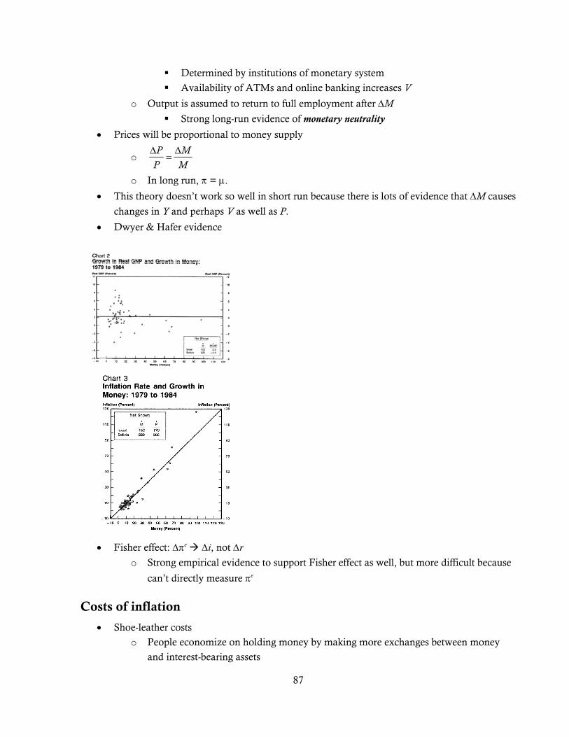
87
Determined by institutions of monetary system
Availability of ATMs and online banking increases V
o Output is assumed to return to full employment after ΔM
Strong long-run evidence of monetary neutrality
• Prices will be proportional to money supply
o P MP MΔ Δ
=
o In long run, π = μ.
• This theory doesn’t work so well in short run because there is lots of evidence that ΔM causes
changes in Y and perhaps V as well as P.
• Dwyer & Hafer evidence
• Fisher effect: Δπe Δi, not Δr
o Strong empirical evidence to support Fisher effect as well, but more difficult because
can’t directly measure πe
Costs of inflation
• Shoe-leather costs
o People economize on holding money by making more exchanges between money
and interest-bearing assets
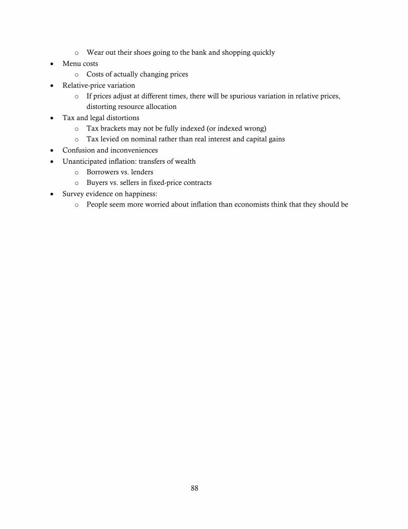
88
o Wear out their shoes going to the bank and shopping quickly
• Menu costs
o Costs of actually changing prices
• Relative-price variation
o If prices adjust at different times, there will be spurious variation in relative prices,
distorting resource allocation
• Tax and legal distortions
o Tax brackets may not be fully indexed (or indexed wrong)
o Tax levied on nominal rather than real interest and capital gains
• Confusion and inconveniences
• Unanticipated inflation: transfers of wealth
o Borrowers vs. lenders
o Buyers vs. sellers in fixed-price contracts
• Survey evidence on happiness:
o People seem more worried about inflation than economists think that they should be
89
Day 36: Aggregate Demand and Supply Note: We are omitting open-economy macroeconomics chapters (18 & 19). These are important and
useful, but we just don’t have time for them. I recommend reading them.
Classical macroeconomics
• Output is at “natural” level
o Unemployment at microeconomic natural rate
o Allocation of resources and output of each commodity determined by micro general
equilibrium
• Price level determined by MV = PY, given Y = Yn, V determined by monetary technology,
and M determined by central bank and banking system
o Inflation is π = μ – g (if V constant over time)
• Real interest rate determined by equilibrium in loanable-funds market
o Nominal interest rate = equilibrium real rate + rate of inflation
• Exchange rate changes in a way to offset relative inflation at home and abroad (we didn’t
study this)
• This is a good picture of the long-run equilibrium of the economy
o Macroeconomy tends to move toward this situation in long run
o Average or trend movements in macroeconomy tend to follow this model
Business cycles
• Shocks can upset the long-run equilibrium of the economy
o There is a distinct pattern to the fluctuations that result from shocks
o This pattern is what we study as business cycles
• We categorize the shocks that affect the economy into two kinds, and build a model to
analyze them
o Aggregate demand shocks: shocks to desired spending
Housing investment stimulated by cheap subprime loans, depressed by
overbuilding and bursting of bubble
Stimulus package
Expansionary monetary policy increases availability of bank loans and
lowers interest rates in short run, reducing costs of investment
o Aggregate supply shocks: shocks to production or costs
Oil-price increases or large wage increases raise costs of production
Improvements to technology lower costs and increase natural level of output
Aggregate demand
• AD curve slopes downward but not for the same reasons as the micro demand curve
90
o No obvious substitution because it is demand for all US goods.
• AD slopes down because of (at least) three effects:
o Wealth effect: P↓ ⇒ M/P ↑ ⇒ real wealth ↑ ⇒ C ↑
o Interest-rate effect: P↓ ⇒ M/P ↑ ⇒ people are holding more real money than they
want to give their spending, interest rates, etc. ⇒ people will try to buy bonds with
their excess money holdings ⇒ equilibrium interest rate on bonds ↓ ⇒ I ↑
o Exchange-rate effect: P↓ ⇒ (if nominal exchange rate doesn’t change) U.S. goods are
cheaper in world markets ⇒ NX ↑
• Shifts in AD
o Shocks (other than income and price) that cause households to change consumption
spending
Wealth shock due to changes in asset prices
Changes in lifetime tax burden
• Note potential importance of Social Security here
General optimism/pessimism
Changes in life expectancy relative to expected working life
Access to credit (real interest rate & ease of lending standards at banks)
o Shocks to investment demand
Expectations about the future profitability of additional capital (MPK)
Changes in the cost of capital (shocks to real interest rate)
• Monetary policy can affect real interest rate in the short run, so this is
one channel of monetary policy effect
• Access to credit may be issue for small businesses (lending standards
at banks)
Changes in tax laws that affect the cost (or productivity) of capital
Technological changes that affect MPK
o Changes in government purchases
o Changes in net exports
Changes in exchange rate: depreciation of dollar ⇒ US goods are cheaper
(given US and foreign prices) ⇒ NX↑
Changes in foreign incomes affect demand for US exports
Aggregate supply
• How does an increase in price of output affect aggregate quantity supplied?
o Each firm’s demand curve and MR curve shift upward
o Effect on output depends crucially on whether costs also changed
If MC also shifts upward by same amount, then no change in output: AS is
vertical
If MC doesn’t shift, then output increases
91
o In long run inflation situation, we expect all prices, wages, costs, etc. to rise together
LRAS is vertical at natural level of output
o In short run, an increase in prices may (or may not) be accompanied by a full
increase in costs
If costs do not rise fully with output, then SRAS slopes upward
• Determinants of natural output (LRAS)
o All the growth accounting stuff:
Size of labor force, amount of human capital, and natural rate of
unemployment
Amount of physical capital and its quality
Availability of imported inputs
Technological capability
o LRAS will shift to the right as growth occurs
Position of LRAS can be thought of as the trend output of the economy
o Long-run equilibrium path of the economy
LRAS moves to the right with growth in natural output
AD shifts upward as money supply grows (and other factors, perhaps)
Sequence of equilibrium points moving to right and perhaps up or down
• Short-run AS
o SRAS slopes upward, intersecting the LRAS at the expected price level
o Multiple theories of why SRAS slopes upward: all complementary
Sticky wages
• Wages are fixed by labor contracts in the short run, so costs don’t go
up and down immediately with prices
• MC doesn’t shift with D and MR, so firms respond to changes in AD
by increasing or decreasing Y
• Contracts expire in the long run, so eventually firms adjust back to
natural Y and increase prices (LRAS is vertical)
Sticky prices
• It is costly for firms to physically change prices (menu costs), so they
may increase or decrease Y in response to short run demand changes
rather than just changing P
• Increased operating profit from staying at MR = MC may be less
than the menu cost
• Eventually menus wear out and they adjust prices, so effect on Y is
only temporary (LRAS is vertical)
Misperception of costs vs. prices
• Firms may have better information about the prices of their outputs
than their inputs
92
• They may see change in MR but not change in MC, so they respond
by changing output in short run
• In long run they learn about their costs, MC changed with MR,
output goes back to natural level (LRAS is vertical)
Effects of macroeconomic shocks
• Demand shocks
o In short run, shocks to AD affect both Y and P
o In long run, only P changes
o How does the short run evolve into the long run?
Change in expected price pushes SRAS up or down
SRAS passes through LRAS at expected price level
SRAS shifts as expected price level adjusts to actual ΔP
o Tradeoff between using AD policy to restore full employment vs. waiting for self-
correction
• Supply shocks
o Shocks to LRAS or just to SRAS?
o To keep simple, let’s think only of SRAS increasing due to increase in imported oil
price or other cost shock
o P ↑ and Y ↓ in short run: stagflation
o Long-run adjustment occurs as expected price changes and/or natural output
changes
93
Day 37: Monetary and Fiscal Policy
Monetary policy and AD
• Keynes’s liquidity preference model
• Demand for real money balances depends on Y and i
o ( ),dM
L Y rP
= or ( ),dM P L Y r= ×
o Assume πe is fixed so we can use r
• Asset-holding balance between demand for money and supply of money
o Supply of money determined by Fed and banking system via money multiplier
o Show graph with money demand vs. supply
o Show effects of increase in P
o Show effects of increase in Ms
o Show effects of equi-proportionate increases in P and Ms
• Change in r ⇒ change in spending, so AD ↑ with increase in money supply
• Fed often targets r rather than M in setting monetary policy, so Ms curve could be horizontal
rather than vertical in the very short run.
• Monetary policy lags: policy can be made very quickly, but takes 6-18 months to have
maximal effect on the economy.
Fiscal policy
• Increase in G or decrease in T = expansionary fiscal policy
o Also increases government deficit
• Increase in G increases spending directly
o Unless AS is vertical (long run), Y increases, which leads to further increase in C via
MPC.
o Process continues because increase in C raises Y and thus C again.
o Each successive increase is smaller by factor of MPC, so process converges
o Ultimate “multiplier” is 1/(1–MPC) = amount of shift in AD
• Multiplier applies to any spending shock, not just G
• Crowding out
o When expansionary fiscal policy raises Y, the demand for money goes up
o Unless money supply curve is horizontal (perfect accommodation by Fed), r ↑.
o The increase in r will curtail some investment and consumption spending
o The increase in government spending “crowds out” some private spending, offsetting
some of the stimulative effect
• Tax cuts
94
o Tax cuts work like spending increases, except that they aren’t direct spending but
instead count on households to increase their spending when T ↓
o Because consumption depends on lifetime income, households are likely to change
spending more if the tax cut is permanent than if it is temporary
(Recall problem set on change in income in both periods vs. just one)
• Fiscal policy lags
o Long lags in recognizing what to do and arguing about how to do it
o Spending may hit the economy rather quickly; multiplier works over time
• Automatic fiscal stabilizers
o Taxes automatically go down (and transfers up) in recessions as base falls
This adds stabilizing policy without need for recognition and decision
Pros and cons of stabilization policy
• Pros
o Policy can help stabilize the economy more quickly than self-correction
o Deflation can be painful mechanism
• Cons
o Policy can be out of phase if not enacted quickly enough
o Hard to know right amount of policy action
o Inflationary bias
Long-run deficits and debt
• Can we run deficits forever?
o Bonds will mature, meaning they have to be repaid
o Repayment means either running a surplus or monetizing
• All government spending must be paid for by current taxes, future taxes, or inflation taxes
• How long can we put off paying off the debt? (Forever?)
o How long will people lend to U.S. government
o Recent crises in Greece and Ireland
o “Credit rating” probably depends on Debt/GDP
o Explain net debt vs. gross debt
Under 60% net debt seems OK with investors
Over 120% seems to get investors very worried
o Show graphs of debt/GDP
95
Day 38: Unemployment-Inflation Tradeoffs
Original Phillips curve
• Show graph
• Top-down, empirical relationship with logical but flawed theory
o When unemployment is low, wages will rise
Modern Phillips curve
• Show graphs
• Flaw in original logic
o Friedman and Phelps, 1968
o Real wages should rise when unemployment is low
o For real wages to rise, wage must rise faster than prices
o For wage setters, this means that wage inflation must be higher than expected price
inflation
o Since wage inflation become price inflation by raising costs, low unemployment will
push inflation higher than expected
• Modern Phillips curve
o Vertical at natural rate in long run
o Downward-sloping in short run
Passes through natural unemployment rate at expected rate of inflation
o Analogy to short-run and long-run AS curves
• Lowering πe improves tradeoff
o WIN buttons
o Price controls
Disinflation in U.S. 1980s
• Could Fed get πe down?
o Apparently not, because unemployment was very high for several years as π↓
• “Sacrifice ratio”
Ending hyperinflations
• Argentina was able to end high inflation with a boom rather than a recession. Why?
o Change of currency effectively cancels contracts, forces new prices, gets people’s
attention.
o If credible, it can change people’s expectations and avoid recession
• Sargent’s evidence on 4 hyperinflations in 1920s
o Credible disinflation relied on credible fiscal stabilization
96
Day 39: The Great Recession
General discussion points
• How could it have been prevented?
o Regulation of lending
o TBTF problems
o Too loose monetary policy for too long
• How effective were the policies that the Fed and the government put in place?
o Compare vs. Great Depression
• What are the appropriate policies going forward?
o More fiscal stimulus?
o Deficit reduction?
o Monetary policy?