class 4: estimation of arma models - jacek suda · class 4: estimation of arma models...
TRANSCRIPT

OLS MLE Estimation AR(1) MA(1) Forecasting ARMA Models Prediction Error Decomposition
Class 4: Estimation of ARMA models
Macroeconometrics - Spring 2011
Jacek Suda, BdF and PSE
April 4, 2011

OLS MLE Estimation AR(1) MA(1) Forecasting ARMA Models Prediction Error Decomposition
Outline
Outline:
1 OLS
2 MLE
3 AR(1)
4 MA(1)
OLS MLE Estimation AR(1) MA(1) Forecasting ARMA Models Prediction Error Decomposition
OLS
For AR(p), OLS equivalent to Conditional MLEModel:
yt = c + φ1yt−1 + . . .+ φpyt−p + εt, εt ∼ WN(0, σ2).= x′tβ + εt, β = φ1, φ2, . . . , φp, xt = yt−1, yt−2, . . . , yt−p
OLS:
β =
(T∑
t=1
xtx′t
)−1 T∑t=1
xtyt,
σ2 =1
T − (p + 1)
T∑t=1
(yt − x′tβ)2.
OLS MLE Estimation AR(1) MA(1) Forecasting ARMA Models Prediction Error Decomposition
Properties
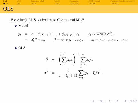
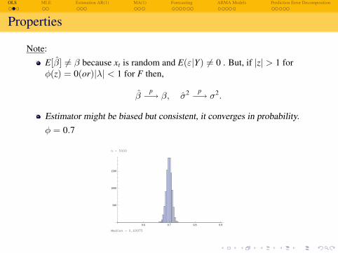
Note:E[β] 6= β because xt is random and E(ε|Y) 6= 0 . But, if |z| > 1 forφ(z) = 0(or)|λ| < 1 for F then,
βp−→ β, σ2 p−→ σ2.
Estimator might be biased but consistent, it converges in probability.φ = 0.7
n = 50
0.6 0.7 0.8 0.9
50
100
150
200
Median = 0.686732
OLS MLE Estimation AR(1) MA(1) Forecasting ARMA Models Prediction Error Decomposition
Properties
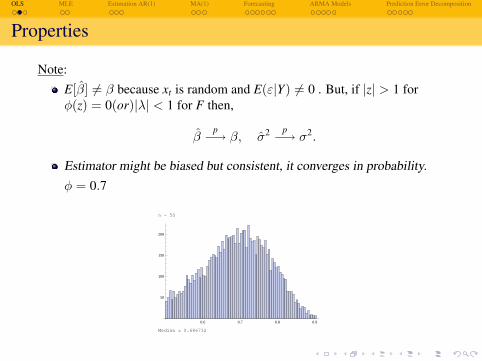
Note:E[β] 6= β because xt is random and E(ε|Y) 6= 0 . But, if |z| > 1 forφ(z) = 0(or)|λ| < 1 for F then,
βp−→ β, σ2 p−→ σ2.
Estimator might be biased but consistent, it converges in probability.φ = 0.7
n = 100
0.6 0.7 0.8 0.9
50
100
150
200
250
300
Median = 0.692907

OLS MLE Estimation AR(1) MA(1) Forecasting ARMA Models Prediction Error Decomposition
Properties
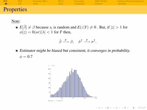
Note:E[β] 6= β because xt is random and E(ε|Y) 6= 0 . But, if |z| > 1 forφ(z) = 0(or)|λ| < 1 for F then,
βp−→ β, σ2 p−→ σ2.
Estimator might be biased but consistent, it converges in probability.φ = 0.7
n = 500
0.6 0.7 0.8 0.9
100
200
300
400
500
600
Median = 0.698815
OLS MLE Estimation AR(1) MA(1) Forecasting ARMA Models Prediction Error Decomposition
Properties
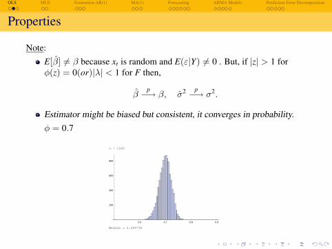
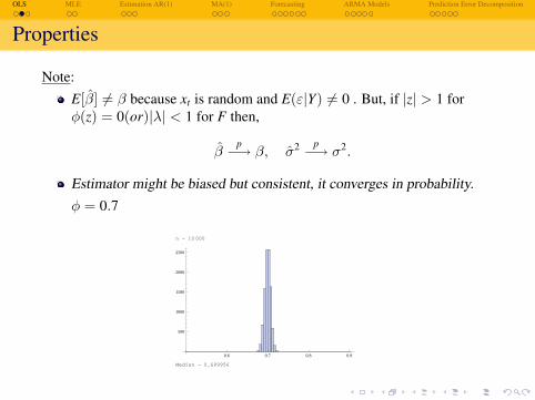
Note:E[β] 6= β because xt is random and E(ε|Y) 6= 0 . But, if |z| > 1 forφ(z) = 0(or)|λ| < 1 for F then,
βp−→ β, σ2 p−→ σ2.
Estimator might be biased but consistent, it converges in probability.φ = 0.7
n = 1000
0.6 0.7 0.8 0.9
200
400
600
800
Median = 0.699796
OLS MLE Estimation AR(1) MA(1) Forecasting ARMA Models Prediction Error Decomposition
Properties
Note:E[β] 6= β because xt is random and E(ε|Y) 6= 0 . But, if |z| > 1 forφ(z) = 0(or)|λ| < 1 for F then,
βp−→ β, σ2 p−→ σ2.
Estimator might be biased but consistent, it converges in probability.φ = 0.7
n = 5000
0.6 0.7 0.8 0.9
500
1000
1500
Median = 0.69975
OLS MLE Estimation AR(1) MA(1) Forecasting ARMA Models Prediction Error Decomposition
Properties
Note:E[β] 6= β because xt is random and E(ε|Y) 6= 0 . But, if |z| > 1 forφ(z) = 0(or)|λ| < 1 for F then,
βp−→ β, σ2 p−→ σ2.
Estimator might be biased but consistent, it converges in probability.φ = 0.7
n = 10 000
0.6 0.7 0.8 0.9
500
1000
1500
2000
2500
Median = 0.699956

OLS MLE Estimation AR(1) MA(1) Forecasting ARMA Models Prediction Error Decomposition
Hypothesis testing
Hypothesis testing:
√T(β − β) d−→ N(0, σ2V−1), V = plimT→∞
1T
T∑t=1
xtx′t .
If we have enough data (T →∞) then t-student will converge toNormal distribution.
tβ=β0 =β − β0
SE(β)∼ t − student(T − 1) −→
T→∞N(0, 1).
See Hamilton for a downward bias in a finite sample, i.e. E[β] < β.
OLS MLE Estimation AR(1) MA(1) Forecasting ARMA Models Prediction Error Decomposition
MLE
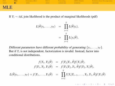
If Yt ∼ iid, join likelihood is the product of marginal likelihoods (pdf)
L(θ|y1, . . . , yT) =T∏
t=1
L(θ|yt),
=T∏
t=1
L(yt|θ),
Different parameters have different probability of generating y1, . . . , yT.But if Yt is not independent, factorization is invalid. Instead, factor intoconditional distributions.
f (Y1,Y2|θ) = f (Y2|Y1, θ)f (Y1|θ),f (Y1,Y2,Y3|θ) = f (Y3|Y2,Y1, θ)f (Y2,Y1|θ),
L(θ|y1, . . . , yT) = f (Y1, . . . ,Y3|θ) =T∏
t=2
f (Yt|Yt−1, . . . ,Y2,Y1, θ)f (Y1|θ)

OLS MLE Estimation AR(1) MA(1) Forecasting ARMA Models Prediction Error Decomposition
MLE
Conditional MLE assumes Y1 fixed (not random). It’s just a simplifyingassumption.
Lc(θ|y1, . . . , yT) =T∏
t=2
f (Yt|Yt−1, . . . ,Y1, θ).
Given normality, first order conditions of maximization Lc are linear inθ.For AR models φCMLE ⇔ OLS.Conditional MLE is consistent. (It’s not so efficient as we ignorerandomness of Y1.)Exact MLE requires non-linear optimization.Often we don’t know distribution of the the data. One thing that isassumed in OLs is the ε ∼ WN.Assuming normality in CMLE is not a bad assumption as we still getconsistent estimator: quasi MLE. (see Davidson and MacKinnon.)We don’t get unbiasness in any of MLE. What can be done is tocompute what the bias is and correct for it.
OLS MLE Estimation AR(1) MA(1) Forecasting ARMA Models Prediction Error Decomposition
Estimation AR(1)
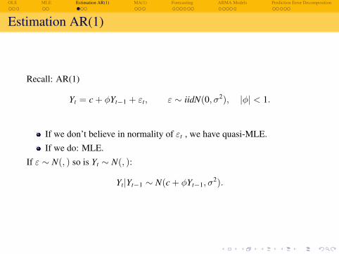
Recall: AR(1)
Yt = c + φYt−1 + εt, ε ∼ iidN(0, σ2), |φ| < 1.
If we don’t believe in normality of εt , we have quasi-MLE.If we do: MLE.
If ε ∼ N(, ) so is Yt ∼ N(, ):
Yt|Yt−1 ∼ N(c + φYt−1, σ2).
OLS MLE Estimation AR(1) MA(1) Forecasting ARMA Models Prediction Error Decomposition
Conditional MLE
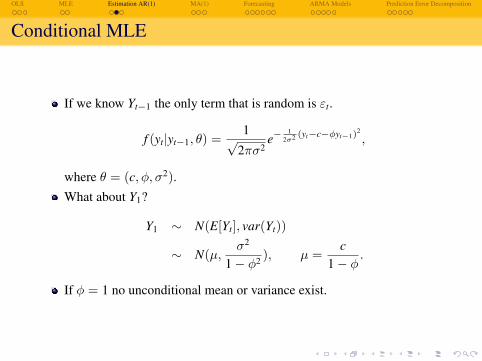
If we know Yt−1 the only term that is random is εt.
f (yt|yt−1, θ) =1√
2πσ2e−
12σ2 (yt−c−φyt−1)
2
,
where θ = (c, φ, σ2).What about Y1?
Y1 ∼ N(E[Yt], var(Yt))
∼ N(µ,σ2
1− φ2 ), µ =c
1− φ.
If φ = 1 no unconditional mean or variance exist.
OLS MLE Estimation AR(1) MA(1) Forecasting ARMA Models Prediction Error Decomposition
Exact MLE
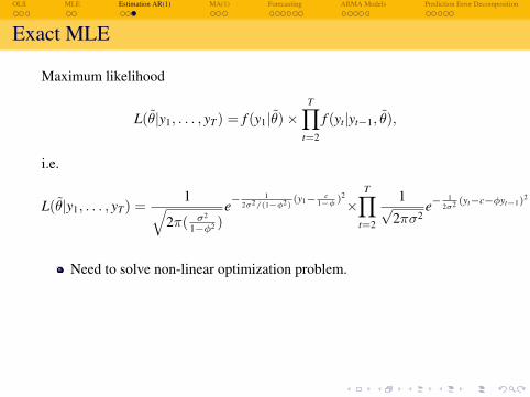
Maximum likelihood
L(θ|y1, . . . , yT) = f (y1|θ)×T∏
t=2
f (yt|yt−1, θ),
i.e.
L(θ|y1, . . . , yT) =1√
2π( σ2
1−φ2 )e−
12σ2/(1−φ2)
(y1− c1−φ )2
×T∏
t=2
1√2πσ2
e−1
2σ2 (yt−c−φyt−1)2
.
Need to solve non-linear optimization problem.

OLS MLE Estimation AR(1) MA(1) Forecasting ARMA Models Prediction Error Decomposition
MA(1)
RecallYt = µ+ ε+ θεt−1, ε ∼ iidN(0, σ2), |θ| < 1.
|θ| < 1 is assumed for invertible representation only, nothing aboutstationarity.
Figure: Bi-model likelihood function for MA process
OLS MLE Estimation AR(1) MA(1) Forecasting ARMA Models Prediction Error Decomposition
Estimation MA(1)
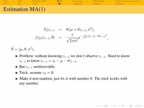
Yt|εt−1 ∼ N(µ+ θεt−1, σ2),
f (yt|εt−1, θ) =1√
2πσ2e−
12σ2 (yt−µ−θεt−1)
2
,
θ = (µ, θ, σ2).
Problem: without knowing εt−2 we don’t observe εt−1. Need to knowεt−2 to know εt−1 = yt − µ− θεt−2.But εt−1 unobservable.Trick: assume ε0 = 0.Make it non-random, just fix it with number 0. The trick works withany number.
OLS MLE Estimation AR(1) MA(1) Forecasting ARMA Models Prediction Error Decomposition
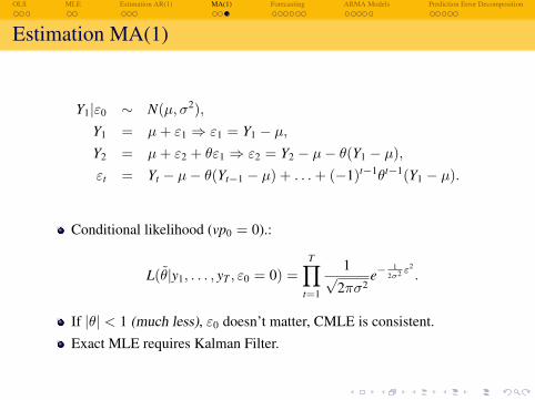
Estimation MA(1)
Y1|ε0 ∼ N(µ, σ2),Y1 = µ+ ε1 ⇒ ε1 = Y1 − µ,Y2 = µ+ ε2 + θε1 ⇒ ε2 = Y2 − µ− θ(Y1 − µ),εt = Yt − µ− θ(Yt−1 − µ) + . . .+ (−1)t−1θt−1(Y1 − µ).
Conditional likelihood (vp0 = 0).:
L(θ|y1, . . . , yT , ε0 = 0) =T∏
t=1
1√2πσ2
e−1
2σ2 ε2
.
If |θ| < 1 (much less), ε0 doesn’t matter, CMLE is consistent.Exact MLE requires Kalman Filter.

OLS MLE Estimation AR(1) MA(1) Forecasting ARMA Models Prediction Error Decomposition
Outline
Outline:
1 Forecasting
2 Linear Projections and ARMA Models
3 Prediction Error Decomposition
OLS MLE Estimation AR(1) MA(1) Forecasting ARMA Models Prediction Error Decomposition
Simple Model
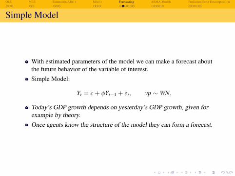
With estimated parameters of the model we can make a forecast aboutthe future behavior of the variable of interest.Simple Model:
Yt = c + φYt−1 + εt, vp ∼ WN,
Today’s GDP growth depends on yesterday’s GDP growth, given forexample by theory.Once agents know the structure of the model they can form a forecast.

OLS MLE Estimation AR(1) MA(1) Forecasting ARMA Models Prediction Error Decomposition
Notation
Denote:Yt – covariance-stationary process, e.g. ARMA(p, q),Ωt – information available at time t,Y∗t+1|t – forecast of Yt+1 based on Ωt.
In our simple model it is Yy+1 given Yt.
OLS MLE Estimation AR(1) MA(1) Forecasting ARMA Models Prediction Error Decomposition
Loss Function
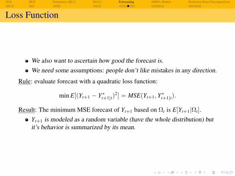
We also want to ascertain how good the forecast is.We need some assumptions: people don’t like mistakes in any direction.
Rule: evaluate forecast with a quadratic loss function:
min E[(Yt+1 − Y∗t+1|t)2] = MSE(Yt+1,Y∗t+1|t).
Result: The minimum MSE forecast of Yt+1 based on Ωt is E[Yt+1|Ωt].Yt+1 is modeled as a random variable (have the whole distribution) butit’s behavior is summarized by its mean.

OLS MLE Estimation AR(1) MA(1) Forecasting ARMA Models Prediction Error Decomposition
Linear Projection
Yt+1 may be very complicated and calculating E[Yt+1|Ωt] might be verycumbersome.If E[Yt+1|Ωt] difficult to compute, use ”best linear forecast”.
Xtp×1 – variables in Ωt “useful” for prediction
Linear projection:
Yt+1|t = α′Xt = α1X1t + . . .+ αpXpt,
where E[(Yt+1 − α′Xt) · Xit] = 0, i = 1, . . . , p.p moments conditions ensure that error is orthogonal to any informationin Ωt:forecast errors are uncorrelated with past information.

OLS MLE Estimation AR(1) MA(1) Forecasting ARMA Models Prediction Error Decomposition
MSE Linear Forecast
Result: The minimum MSE linear forecast of Yt+1 is linear projection.For Gaussian (Normal) process: E[Yt+1|Ωt] = Yt+1|t.Linear projection is optimal in Gaussian case.How do we deal with αs ?
Yt+1|t = α′Xt can be thought of as computed by OLS but bp−→ α, i.e.
OLS estimate, b, converges in probability to true value, α.
Optimality is defined in terms of quadratic loss function.
OLS MLE Estimation AR(1) MA(1) Forecasting ARMA Models Prediction Error Decomposition
ARMA Models
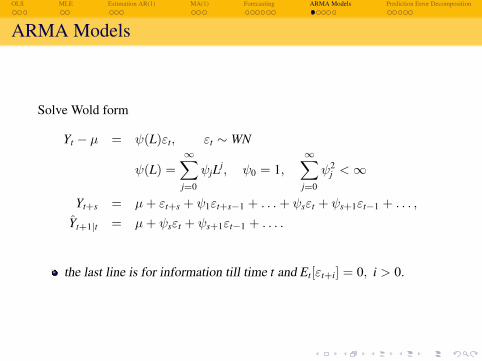
Solve Wold form
Yt − µ = ψ(L)εt, εt ∼ WN
ψ(L) =∞∑
j=0
ψjLj, ψ0 = 1,∞∑
j=0
ψ2j <∞
Yt+s = µ+ εt+s + ψ1εt+s−1 + . . .+ ψsεt + ψs+1εt−1 + . . . ,
Yt+1|t = µ+ ψsεt + ψs+1εt−1 + . . . .
the last line is for information till time t and Et[εt+i] = 0, i > 0.
OLS MLE Estimation AR(1) MA(1) Forecasting ARMA Models Prediction Error Decomposition
ARMA Models
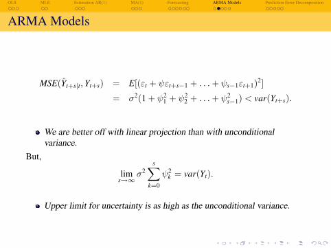
MSE(Yt+s|t,Yt+s) = E[(εt + ψεt+s−1 + . . .+ ψs−1εt+1)2]
= σ2(1 + ψ21 + ψ2
2 + . . .+ ψ2s−1) < var(Yt+s).
We are better off with linear projection than with unconditionalvariance.
But,
lims→∞
σ2s∑
k=0
ψ2k = var(Yt).
Upper limit for uncertainty is as high as the unconditional variance.
OLS MLE Estimation AR(1) MA(1) Forecasting ARMA Models Prediction Error Decomposition
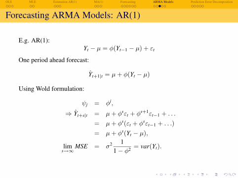
Forecasting ARMA Models: AR(1)
E.g. AR(1):Yt − µ = φ(Yt−1 − µ) + εt
One period ahead forecast:
Yt+1|t = µ+ φ(Yt − µ)
Using Wold formulation:
ψj = φj,
⇒ Yt+s|t = µ+ φsεt + φs+1εt−1 + . . .
= µ+ φs(εt + φsεt−1 + . . .)= µ+ φs(Yt − µ),
lims→∞
MSE = σ2 11− φ2 = var(Yt).
OLS MLE Estimation AR(1) MA(1) Forecasting ARMA Models Prediction Error Decomposition
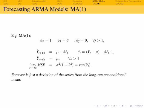
Forecasting ARMA Models: MA(1)
E.g. MA(1):ψ0 = 1, ψ1 = θ, , ψj = 0, ∀j > 1,
Yt+1|t = µ+ θεt, εt = (Yt − µ)− θεt−1,
Yt+s|t = µ, ∀s > 1
lims→∞
MSE = σ2(1 + θ2) = var(Yt).
Forecast is just a deviation of the series from the long-run unconditionalmean.
OLS MLE Estimation AR(1) MA(1) Forecasting ARMA Models Prediction Error Decomposition
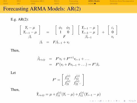
Forecasting ARMA Models: AR(2)
E.g. AR(2):[Yt − µ
Yt−1 − µ
]βt
=
[φ1 φ21 0
]F
[Yt−1 − µYt−2 − µ
]βt−1
+
[εt
0
]vt
βt = Fβt−1 + vt
Then,
βt+s|t = Fsvt + Fs+1vt−1 + . . .
= Fs(vt + Fvt−1 + . . .) = Fsβt.
Let
Fs =
[f (s)11 f (s)
12
f (s)21 f (s)
22 .
]Then,
Yt+s|t = µ+ f (s)11 (Yt − µ) + f (s)
12 (Yt−1 − µ)
OLS MLE Estimation AR(1) MA(1) Forecasting ARMA Models Prediction Error Decomposition
Kalman Filter
Forecasts based on Wold form assume infinite number of observations.We don’t have them in reality.Kalman filter calculates linear projections for finite number ofobservations,
exact finite sample forecast,allow for exact MLE of ARMA models based on Prediction ErrorDecomposition.
OLS MLE Estimation AR(1) MA(1) Forecasting ARMA Models Prediction Error Decomposition
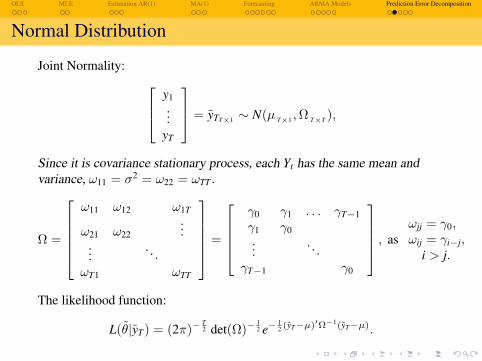
Normal Distribution
Joint Normality: y1...
yT
= yTT×1 ∼ N(µ T×1 ,Ω T×T ),
Since it is covariance stationary process, each Yt has the same mean andvariance, ω11 = σ2 = ω22 = ωTT .
Ω =
ω11 ω12 ω1T
ω21 ω22...
.... . .
ωT1 ωTT
=
γ0 γ1 . . . γT−1γ1 γ0...
. . .γT−1 γ0
, asωjj = γ0,ωij = γi−j,
i > j.
The likelihood function:
L(θ|yT) = (2π)−T2 det(Ω)−
12 e−
12 (yT−µ)′Ω−1(yT−µ).

OLS MLE Estimation AR(1) MA(1) Forecasting ARMA Models Prediction Error Decomposition
Factorization
Note that for large T Ω might be large and difficult to invert.Since Ω is positive definite symmetric matrix then there exists a unique,triangular factorization of Ω,
Ω = AfA′,
where
f T×T =
f1 0 · · · 0
0 f2...
.... . .
0 · · · fT
, ft > 0 ∀t diagonal matrix
A T×T =
1 0
a21 1...
. . .aT1 aT2 . . . 1
.
OLS MLE Estimation AR(1) MA(1) Forecasting ARMA Models Prediction Error Decomposition
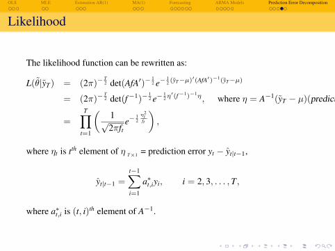
Likelihood
The likelihood function can be rewritten as:
L(θ|yT) = (2π)−T2 det(AfA′)−
12 e−
12 (yT−µ)′(AfA′)−1(yT−µ)
= (2π)−T2 det(f−1)−
12 e−
12η′(f−1)−1η, where η = A−1(yT − µ)(prediction error)
=T∏
t=1
(1√2πft
e−12η2
tft
),
where ηt is tth element of η T×1 = prediction error yt − yt|t−1,
yt|t−1 =t−1∑i=1
a∗t,iyi, i = 2, 3, . . . ,T,
where a∗t,i is (t, i)th element of A−1.
OLS MLE Estimation AR(1) MA(1) Forecasting ARMA Models Prediction Error Decomposition
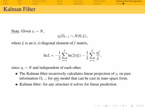
Kalman Filter
Note: Given yt ∼ N,ηt|Ωt−1 ∼ N(0, ft),
where ft is an (t, t) diagonal element of f matrix,
ln L = −12
T∑t=1
ln(2πft)−12
T∑t=1
η2t
ft,
since ηt ∼ N and independent of each other.The Kalman filter recursively calculates linear projection of yt on pastinformation Ωt−1 for any model that can be cast in state-space form.Kalman filter: for any structure it solves for linear prediction.