citizens and governance in a knowledge-based society · compensation, such as leaves (vacation,...

Project no: 028412

AIM-AP

Accurate Income Measurement for the Assessment of Public Policies

Specific Targeted Research or Innovation Project

Citizens and Governance in a Knowledge-based Society

Deliverable 1.4b Home production and fringe benefits in Italy

Due date of deliverable: January 2008 Actual submission date (revised version): April 2008

Start date of project: 1 February 2006 Duration: 3 years Lead partner: European Centre Vienna Revision [First revision]

Conchita D'Ambrosio Università di Milano-Bicocca and DIW, Berlin

and

Chiara Gigliarano Università Politecnica delle Marche, Ancona

Home production and fringe benefits: an estimation of their distributional impact in Italy AIM-AP Project 1 – Non-cash incomes

Second version: April 2008

2

CONTENTS

1. Introduction 3

2. Results from other studies 4

3. Data 5

3.1. SILC 2004 5

3.2. SHIW04 7

3.3. Use of Time 2002-2003 8

4. Analysis of Company Cars 8

4.1. Tax issue on Company Cars 8

4.2. Distributional effects of Company Cars 9

5. Analysis of Fringe Benefits 14

5.1. Methodological issues: imputation of fringe benefits in SILC04 15

5.2. Distributional effect of fringe benefits 17

6. Analysis of Home Production 18

6.1. Methodological issues: imputation of home production in SILC04 21

6.2. Distributional effect of home production 23

7. Concluding remarks 34

8. References 35

9. Appendix A: Econometric results 37

10. Appendix B: ACI’s tables 40

3

1. Introduction A growing literature has been arguing in favour of measures of income that incorporate

valuations of non-monetary and in-kind resources; see, e.g., Smeeding et al. (1993). The reason

for considering an extended definition of income rather than the simple monetary income is that the

former provides a better measure of a person’s well-being and access to economic resources.

In this paper we focus on two specific types of in-kind income, i.e. the ones related to goods

and services that are provided either by the employer or by own (non-farm) production. In

particular, the measures of extended income that are considered in this paper combine household

monetary income data and valuations of fringe benefits and home production.

Empirical analyses of these extended income measures, using Italian data, are rare and this

paper aims to provide new estimates of the distribution of such extended income, following the

“welfare economics” approach, which analyzes the impact of fringe benefits and home production

on the individual equivalised income.

The data set that we use as baseline cash income is SILC 2004 (“Survey on Income and

Living Conditions”) data set, which contains information only on a specific kind of fringe benefits,

that is company cars. In the data set SHIW04 (“Survey on household income and wealth”),

provided by the Bank of Italy for the year 2004, the definition of the total household disposable

income includes already the measure of fringe benefits (such as luncheon vouchers, trips and

company cars) and, therefore, any analysis based on such total net income takes already into

account the in-kind benefits provided by the employer; however, very few are the studies that

specifically analyze the impact of the component “fringe benefits” on the overall household net

income. For that reason, we present two different analyses related to fringe benefits, one that

studies the effect on the income distribution of the sole type of fringe benefits included in SILC

2004 dataset, i.e. the company cars. The second analysis, instead, adds to the baseline cash

income in SILC 2004 the variable “fringe benefits” included in SHIW04; we use, in particular, data

matching methods, by estimating models of employee fringe benefits with data from SHIW04 and

using the estimates to impute fringe benefits values to respondents to the SILC 2004.

At the same time, the reference data set SILC 2004 does not contain any kind of information

on home production; therefore, we have to use data matching methods also in this analysis. As in

Jenkins and O’Leary (1996), we estimate the extend and the monetary value of home production

through time use data. We employ the survey on Use of Time 2002-2003 carried out by the Italian

National Institute of Statistics (ISTAT), which contains detailed data on the time spent in domestic

work activities. A third analysis is therefore conducted in this paper, aiming at studying the effects

on the income distribution of household production. Lastly, we discuss the joint distributional

impact of fringe benefits and home production.

4

The paper is structured as follows: after a brief review, in the next section, on the main

results from other studies on fringe benefits and home production, and after a description of the

data sets in Section 3, we analyze in Section 4 the distributional effects of company cars, in

Section 5 the impact of fringe benefits and in Section 6 the effects of home production. Section 7

concludes.

2. Results from other studies In this section, we briefly review the literature on fringe benefits and on home production.

The literature on fringe benefits rarely focused on the impact of such employer-provided in-

kind transfers on the distribution of income and the few papers on such topic refer mainly to the

U.S. situation; see, e.g., Pierce (2001) and Chung (2003).

Pierce (2001) focused on the changes of inequality in the distribution of employer-provided

fringe benefits in the United States. His definition of fringe benefits is quite wide, including both

legally required benefits, such as Social Security and Medicare, and voluntary non-wage

compensation, such as leaves (vacation, holidays, sick leave), health-, life- and sickness-

insurance, retirement and savings. He showed that the level of inequality in the distribution of

worker compensation is higher when voluntary fringe benefits are included in the definition of

compensation than when the sole monetary wage is considered. Moreover, “the fringe benefits

have become less equally distributed through time, and compensation inequality rose over the past

10-15 years by a greater amount than did wage inequality” (Pierce, 2001, p. 1520).

Chung (2003) was interested in measuring the inequality in the wage distribution in the U.S.

both with and without the inclusion of fringe benefits; his study showed that when fringe benefits

are taken into account, inequality increases. He concluded that analysis based only on wages

tends to overestimate inequality among the skilled workers, to underestimate the inequality among

the less skilled and to underestimate inequality in the labor market. Greater inequality growth over

time results primarily from the disproportionately greater decline in health insurance coverage for

the less skilled workers.

To the best of our acknowledge, no scientific studies have been produced yet that analyze

the distributional impact in Italy of including fringe benefits into the income’s definition. This paper

may constitute one of the first attempts to fill this gap.

Regarding home production, Jenkins and O’Leary (1996) combined household money

income data and valuations of household production time, analysing the distribution of such

extended income among non-elderly, one-family households in the U.K.. Their results showed that

the extended income distribution is substantially more equal than money income. In particular,

families without earners are shifted up the distribution relative to families with earners, so that the

5

income differential reduces significantly, thought the former group remains poorer on average.

Moreover, single persons are shifted down the distribution relative to married couple families.

For the Italian situation, Monti (2007) carried out an analysis on differences in the use of time

between males and females; in particular, Italian males spend most of their time in paid work, while

Italian females focus their time mainly on unpaid household work, such as housework, errands,

child and elderly care. Such gender difference is common to other countries analysed, such as

Germany, Netherlands, Italy and U.S., but the gap between men and women remains greater in

Italy. Monti (2007), moreover, proposed an estimate of the total value of domestic work, by

multiplying the time spent in such kind of activities to the gross hourly wage estimated by Eurostat,

differently for male (8.76 €) and female (6.94 €). The total value of domestic work time has been

estimated equal to 432 billion Euro, corresponding to 33% of the Italian GDP. The cited work,

however, did not analyze the impact of such evaluated home production on income distribution.

3. Data The reference dataset that contains the baseline cash income, to which we will add the fringe

benefits value, is SILC 2004 (“Survey on Income and Living Conditions”). However, such dataset

contains information only on a specific type of fringe benefits, company cars (henceforth, CC).

Therefore, we prefer to enrich the analysis on fringe benefits by considering also a slightly richer

dataset, SHIW 2004 (“Survey on Household Income and Wealth”), which contains information on

further types of employer-provided fringe benefits (company cars, luncheon vouchers, trips, etc.

(excluding housing)).

About home production, no information is included in the dataset SILC 2004; we will,

therefore, match the reference data set with the Use of Time 2002-2003 data set, that contains

detailed information on the use of time in Italy.

Let us briefly describe the main features of the three datasets.

3.1 SILC 2004 The reference dataset employed for the analysis is the “IT-SILC XUDB 2004-versione

Novembre 2007”, which contains the Italian data of the European Survey of Income and Living

Conditions (EU-SILC), based on the European Union Regulation (no. 1177/2003) which defines

the EU-SILC project. In particular, it contains extra variables beyond the ones common to all the

European countries that are part of the project.

This survey replaces the former European Community Household Panel (ECHP) with the

main scope to provide, through harmonized definitions and methods, comparable data, cross-

6

sectional and panel, in order to analyse jointly income and welfare distribution among the

households and to monitor the effect of European and national socio-economic policies.

The sample design of the Italian SILC consists of a two-stage sampling, according to which,

for each region, municipalities are first divided into the auto-representative municipalities (with

larger population size) and the non auto-representative municipalities (smaller in size). All the auto-

representative municipalities belong to the sample and within them households are systematically

drawn from the register office records. For the non auto-representative municipalities, a sample

design with two stages is conceived, according to which a sample of municipalities is chosen (first

stage) and households are selected randomly within each municipality, from the register office

records (second stage). The probability of selecting a municipality is proportional to its population

size, while households are drawn with the same probability.

The Italian EU-SILC sample contains 24,204 households and 61,429 individuals (52,509

aged 15 and more years old at the end of the referring income period of time) living in 731

municipalities. For all the analyses in this paper the population of interest will be composed by all

individuals living in private households with positive disposable income; therefore, we reduce to

24,048 households and 61,107 individuals.

In EU-SILC 2004 information on income refer to the year 2003, while information on the living

conditions refer to the moment of the interview, i.e. the year 2004. In order to define the baseline

income we consider the total household disposable income “HY020”, given by the sum, for all

household members, of gross personal income components (including company cars for private

usage), gross cash benefits (self-employment, sickness, survivor, unemployment, disability),

income from rental of property, family allowances, housing allowance, interests and profits from

capital investments, minus taxes on income, wealth, social insurance contributions. The baseline

cash income for the exercise of this paper is then defined as the total household disposable

income “HY020” minus the amount of company cars (variable “PY020N”).

The variable “PY020N” refers to the non-monetary income components which may be

provided free or at reduced price to an employee as part of the employment package by an

employer. For the year 2004 only the company car are part of this variable.

An exact definition of Company Car (i.e. of the variable PY020N) is provided by Eurostat

(2006): “Company cars and associated costs (e.g. free fuel, car insurance, taxes and duties as

applicable) provided for either private use or both private and work use. (…) The value of goods

and services provided free shall be calculated according to the market value of these goods and

services. The value of goods and services provided at reduced price shall be calculated as the

difference between the market value and the amount paid by the employee.”

The approach used in the Italian version of SILC, for imputing the value of the Company Car,

is indirect, in sense that it is based on information on characteristics of the car asked to the

respondents, such as the type and brand of the car and the year of construction. In particular, the

7

respondent was asked: “During the year 2003, has your employer provided you with a car, a van or

other motor vehicle also for your personal usage?” and, if yes, “Which type of vehicle is it and for

how many months have you used it during the year 2003 for your personal needs?”.

The information obtained from the questionnaire is then used to evaluate the benefit derived

from the company car, by following the rules of ACI (“Automobile Club d’Italia”). ACI provides

tables that include the cost per km of the company car, distinguishing among different types of fuel

used by the car (gasoline, diesel oil, methane) and different types and the series of cars. The total

value of the company car is estimated equal to such cost per km times 15,000 km, which is the

annual distance that conventionally is attributed by law to every company car. The value of the

corresponding fringe benefits equals 30% of the estimated cost of the company car, i.e. the

specific cost per km times 4,500 km1. See Appendix B for an example of ACI’s tables referring to

the year 2003.

3.2. SHIW04

The second data set employed is the 2005 Survey provided by the Bank of Italy on the 2004

Household Income and Wealth (SHIW04). During the period between May and September 2005,

families have been interviewed about their income, wealth and other socio-economic conditions,

regarding the preceding year. The data set is made up by 20,581 individuals grouped in 8,012

households, representative of the whole Italian population (58.2 millions of individuals and 22.6

millions of households). The sample design of the SHIW04 data set consists of a two-stage

sampling, according to which municipalities are first divided into strata and, then, for each strata, a

sample of municipalities is chosen (first stage) and households are selected randomly within each

municipality, from the register office records (second stage).

The number of respondents that are employees, both as main activity and as secondary

activity, is 6,014. In such a survey several information are collected on the characteristics of these

category of workers, such as number of hours of paid overtime, kind of contract, number of people

regularly employed in the firm and so on.

In particular, the employees were asked the following: “In 2004 did you receive fringe benefits

in the form of luncheon vouchers, trips, company cars, etc. (excluding housing)?” and, if yes, “What

was the monetary value of these benefits?”.

The variable of interest in such a dataset is “ylnm”, i.e. the monetary value of such fringe

benefits received. It should be noticed that according to Biancotti et al. (2004), the quality of the

data collected in the survey SHIW04 is quite good for the employee’s income, but it is worse for

information on non-monetary income, such as the fringe benefits.

1 Starting from the year 2007, the value of the fringe benefit corresponds to 50% of the total value of the company car, i.e. the specific cost per km times 7,500 km.

8

3.4. Use of Time 2002-2003

The third data set employed is the Survey on Use of Time 2002-2003 (“Indagine Multiscopo

sulle famiglie- Uso del Tempo”) carried out by the Italian National Institute of Statistics (ISTAT).

During the period between April 2002 and March 2003, families have been interviewed mainly

about their use of time. The sample is made up by 55,773 individuals grouped in 21,075

households, representative of the whole Italian population (58.2 millions of individuals and 22.6

millions of households). The sample design of the SHIW04 data set consists of a two-stage

sampling, according to which municipalities are first divided into strata and, then, for each strata, a

sample of municipalities is chosen (first stage) and households are selected randomly within each

municipality, from the register office records (second stage).

The basic unit of the survey is the household, defined as either one person living alone or

people (who may or may not be related) living together. Persons living in collective households and

in institutions are excluded from the target population.

One-day time diaries were completed by all the household components aged 3 or more

years; parents filled the diaries for the youngest children. Respondents have been asked to fill the

diary at a prefixed day, either weekday or weekend day, describing the activities that they have

performed during the day as well as where and with whom they have carried out such activities.

ISTAT then coded such information in order to get homogeneous data. The survey provides also information on socio-economic characteristics of the household

components, such as age, gender, educational level attained, occupation.

The individual time of interest for our analysis is the “domestic work time", that is time for

food preparation, housework, odd jobs about home, gardening, repairs, do-it-yourself jobs,

shopping, child care, plus domestic travel associated with these activities. Excluded from the

definition of domestic work are hobbies and leisure activities, paid work related activities. Our

analysis considers domestic work carried out during working weekday as well as during weekends.

4. Analysis of Company Cars

In this section we focus on a particular type of fringe benefits: company car. In the

following, we first briefly describe the Italian taxation system for company cars and then we

analyze the impact of company cars on the distribution of income.

4.1. Tax issue on company cars

The Italian taxation on company cars is different according to the degree of usage of such a

car by the employee. If the company car is provided by the employer only for job activities, then the

9

use of the company car does not determine a fringe benefit. If the company car is only for private

use, the value of fringe benefit is determined according to the cost of renting that type of car.

If the company car is allowed for a mixed usage, both for the job activities and for personal

use, then the fringe benefit is determined independently of the kilometers actually covered or of the

costs actually paid for the car. For this situation, the taxation of company cars refers to the law DL

n. 314 02/09/1997, according to which the value of the company car has to be obtained multiplying

15,000 km by a fixed amount per km (provided by ACI); independently of the effective use of the

company car, the fringe benefits is fixed equal to 30% of the company car’s value.

From such amount the eventual costs already paid by the employee for the company car

have to be deducted.

The fringe benefits are part of the taxable income from which calculating social and public

welfare contributions and personal income taxes. Obviously, if the amount of money paid by the

employee for the usage of the company car equals or exceeds the amount obtained from the ACI’s

tables, then the benefit is completely null.

From the point of view of the employer, costs related to the company car are deductable (for

the taxes IRES, IRPEF and IRAP); if the company car is allowed for a mixed usage for the entire

year, then the costs are completely deductable, otherwise they are partly deductable.

Recently, the law n. 286 24/11/2006 has modified the evaluation of company cars; the

proportion of the company car’s value that corresponds to the fringe benefits moves from 30% to

50%; see, e.g., Gaiani (2006).

4.2 Distributional effects of company cars

Let us now study how the introduction of the company car’s value into the definition of income

modifies the income distribution. Obviously, the potential beneficiaries of company cars

(henceforth, CC) are the sole employee workers; we consider as employee any worker who

receives income coming from a work as an employee (this can be the main or the secondary

working activity).

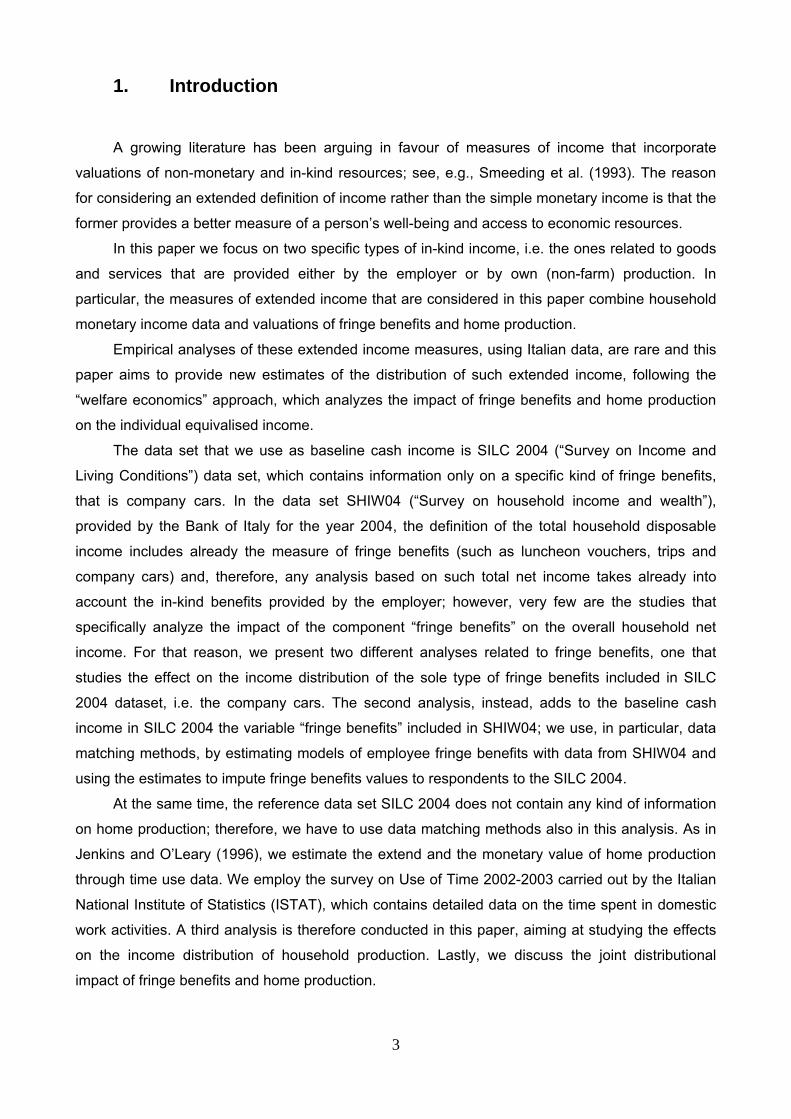
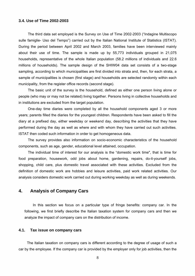
Figures 1 and 2 show the distribution of company cars among, respectively, all the employees

(grossed up to the population) and among different categories of employees.

10

Figure 1: Percentage of company car’s beneficiaries among the employees

Source: own elaboration of SILC 2004

Figure 2: Percentage of company car’s beneficiaries among different categories of employees


11

The incidence of CC over all the Italian employees is quite low (2.2%) and the proportion of

CC beneficiaries is much higher for managers than for cadres and office workers.2

Table 1 shows that the proportion of beneficiaries increases with income and the average

mean of the company car’s value, calculated over the sole beneficiaries, equals 1,448 €.

Table 1: Distribution of beneficiaries and of CC mean, by income quintile

(non equivalent) mean of CC (€)

Quintile

% of beneficiaries

among employees among the employees among CC beneficiaries

1 0.85 10 1,215

2 1.43 16 1,105

3 1.22 17 1,357

4 1.93 24 1,246

5 4.43 73 1,638

Total 2.22 32 1,448

Source: own elaboration of SILC04

If we do not restrict the attention only to employees, we can analyse the incidence of CC over

the entire Italian population; Table 2 shows that in the year 2003 only 0.67% of the entire

population benefits from company cars, corresponding to 385,392 beneficiaries.

Table 2: number in the population (N), in the sample (n) and portion (%) of CC beneficiaries

Beneficiaries N n %

no 57,213,271 60,672 99.33

yes 385,392 435 0.67

Total 57,598,663 61,107 100


From Figure 3 it appears that the proportion of CC beneficiaries increases with income: only

0.14% of Italians in the first income quintile benefits personally from CC, while 1.74% of Italians in

the highest income quintile receives a company vehicle from the employer.

2 The remaining categories of employees, in particular the blue collar, have not been included in the representation of Figure 2 since almost all of them do not possess a company car.

12

Figure 3: Proportion (in %) of CC beneficiaries by income quintile


If we pool and share equally the CC benefits within each household, we see, from Tables 3,

that 98% of Italians lives in households that do not receive any company car, 1.96% of individuals

lives in households with one CC’s beneficiary and only 0.04% lives in a family with 2 beneficiaries.

Table 3: Distribution of people (Number over the entire population (N), number of the sample (n) and proportion (%)), by number of CC beneficiaries within the HH

N. of beneficiaries within HH N N %

0 56,446,769 59,772 98

1 1,126,329 1,298 1.96

2 25,565 37 0.04

Total 57,598,663 61,107 100


Figure 4 shows that the proportion of people living in a household that receives at least a

company car increases considerably with income.

Figure 4: Proportion (in %) of people living in HH with one or more CC, by income quintile


13

Therefore, it appears that in Italy the provision of company cars by the employers is not a

very widespread phenomenon and, moreover, most of the CC beneficiaries are located in the

upper part of the income distribution.

Let us consider now how the income distribution changes when we add to the monetary

income the company car’s benefits.

The population of interest is composed by all individuals living in private households with

positive disposable income. In order to take into account the differences in needs among

households with different sizes, we apply the modified OECD scale for both disposable income and

transfers due to such fringe benefit.

Table 4: Changes in income share and disposable income after CC transfer, by income quintile.

INCOME SHARE

QUINTILE Baseline with CC

% increase in

disposable income

mean transfer per

capita (in €)

1(bottom) 7.45 7.44 0.04 2

2 12.74 12.73 0.06 5

3 17.12 17.12 0.07 9

4 22.61 22.60 0.09 15

5 (top) 40.09 40.10 0.15 45

ALL 100.00 100.00 0.10 15


Table 4 shows that the income share slightly reduces in the lowest income quintiles and

slightly increases in the highest income quintile; moreover, the table shows that the percentage

increase in disposable income rises with income and the same occurs for the mean absolute

transfer.

Table 5: Inequality change due to CC


VALUE OF THE INDEX

Baseline Including CC % change

Gini 0.325 0.325 0.1

Atkinson 0.5 0.091 0.091 0.1

Atkinson 1.5 0.271 0.272 0.1

MLD 0.193 0.193 0.1

FGT0 0.187 0.186 -0.1

FGT1 0.055 0.055 0.0

FGT2 0.027 0.027 0.0

14

As expected, Table 5 shows that the introduction of the CC’s benefit implies a slight increase

in inequality; moreover the poverty rate slightly reduces while no change takes place in the other

poverty indices.

Therefore, our findings are coherent with the ones obtained in Frick et al. (2006), according to

which the inclusion of CC in the overall employee’s compensation measure yields higher degree of

inequality.

5. Analysis of Fringe Benefits

We now turn to consider not only the employer-provided benefits constituted by company

cars, but also other types of fringe benefits, such as luncheon vouchers, trips, etc., excluding

housing. Since in SILC 2004 such information is not available (but it will be available starting from

the survey SILC 2007), we exploit a second data set, SHIW04, which includes, as already pointed

out, the variable of fringe benefits “ylnm”. The group affected by the fringe benefits is the group of

employees; for that reason, we first study some basic characteristics of such group.

Table 6 shows that, according to the data set SILC 2004, 30.27% of Italians is an employee

worker, corresponding to about 17,5 millions individuals, while, according to the SHIW04 data set,

such numbers are slightly higher: 31% of the population, corresponding to 18 millions individuals,

receives a wage for an employee job.

Table 6: Description of employees in SHIW and SILC Employee n N %

SILC

No 42,699 40,407,491 69.73

yes 18,730 17,544,798 30.27

Total 61,429 57,952,289 100

SHIW

No 14,608 40,218,093 69

yes 6,014 18,067,972 31

Total 20,622 58,286,065 100

Source: own elaboration of SILC 2004 and SHIW04

15

Figure 5: Percentage mean of employees by income quintile


Figure 5 reveals an increasing trend in the proportion of employees as income increases, on

average. It means that most of the employees are concentrated in the highest income quintiles.

5.1. Methodological issues: imputation of fringe benefits in SILC04

SILC 2004 is our source of data on monetary incomes of households; it contains also

information on a wide range of employees characteristics and we exploit this in our data matching

as well as in our income distribution breakdowns.

Since the information on fringe benefits (henceforth FB) is contained in the SHIW04 data set,

we have to impute fringe benefits values provided by the respondents of SHIW04 to respondents

of the survey SILC 2004, using regression matching methods. Such imputation is obviously

restricted to the group of employee workers. First we deflate the value of FB in SHIW04 with

respect to the year 2003.

We adopt a two-steps regression, in such a way that we first control for the percentage of the

employees that receive the fringe benefits and then we impute only to them the value of fringe

benefits.

We can synthesize the method that we have adopted through the following steps:

First, we choose a set of covariates (in particular, characteristics of the employee) that are

common to the both data sets and we make them comparable; such covariates, listed in

Appendix A, will be indicated as XSHIW and XSILC for the two data sets, respectively.

We then run a probit regression, for the dataset SHIW04, of the probability of receiving the

fringe benefits (FB) with respect to the covariates (XSHIW), restricted only to the employees;

let us call P the dummy variable

16

.

Therefore, the probit model is:

probit(P)=β’ XSHIW +ε, ε~N(0,σ2).

We use the coefficients of such probit regression to predict the probability P̂ of receiving a

positive FB for all the employees in the dataset SILC 2004:

In order to identify the imputed beneficiaries of fringe benefits in the SILC2004 data set, we

establish that the proportion of FB beneficiaries among the employees has to be the same

in SHIW04 data set and in SILC 2004 data set. Since in SHIW04 8.02% of all the

employees receives a positive fringe benefits, the imputed FB beneficiaries in SILC 2004

will be, therefore, the 8.02% of the employees with the highest fitted probability

We then run a OLS regression, for the SHIW04 dataset, of the amount of fringe benefits

(FB) on the set of common covariates XSHIW, restricted to the FB beneficiaries:

~N(0,τ2).

Finally we use the OLS coefficient in order to predict, in SILC 2004 dataset, the amount of

FB, restricting only to 8.02% of the employees with the highest fitted probability, i.e. to the

imputed FB beneficiaries; the prediction’s model is:

δα ˆ'ˆˆ += SILCXBF .

Note that we assume independence between the residuals of the two regression models, i.e.

between ε and δ.

If the fitted value of FB is negative, we put it equal to 0.

We also assume that the fringe benefits are pooled and shared equally within each

household; each person is imputed with the equivalent fringe benefits of the household to which

she belongs. We apply the same equivalisation and weighting methods to money income and to

fringe benefit values, according to the modified OECD equivalence scale.

17

5.2. Distributional effects of Fringe Benefits

The results of the exercise of adding the imputed fringe benefits to the disposable cash

income are illustrated in Tables 10 to 19.

From Table 10 we can observe that the distribution of the fringe benefits is very unequal and

is concentrated mostly in the highest income quintile: less than 5% of the beneficiaries belongs to

the poorest three quintiles, while more than 95% of the beneficiaries are in the two richest quintiles.

Looking at the share of population with positive fringe benefits in Table 11, 6% of the entire

population lives in a households that receives FB; the population share of beneficiaries increases

with income: only 0.15% of the individuals in the first quintile lives in households that include

beneficiaries, while more than 20 % of the people in the richest quintile receive positive FB.

Table 12 shows that, when the fringe benefits is added to cash income, the income share

reduces in the first four quintiles and increases in the highest quintile, inducing a more unequal

distribution of income. From Table 13 we observe that the mean income increases slightly for the

first quintiles and more considerably for the highest ones. On average, the percentage increase of

income is equal to 0.59% (corresponding to 88 €) and such augment increases with income.

As shown above, fringe benefits are less common among lower incomes. Hence, we would

expect inequality to increase once including a measure of fringe benefits and this increase should

be greater when using inequality measures which are sensitive to changes in the upper part of the

income distribution (e.g. half SCV). Such expectation is confirmed in Table 14, which shows that,

according to the different inequality and poverty indices considered, both inequality and poverty

slightly increases when the amount of fringe benefits is added to cash disposable income.

In Tables 15 to 19 the impact of fringe benefits is decomposed by subgroups of the

population, according to different partitions. Table 15 shows that, after the introduction of FB, the

income increases mainly for young couples with or without children, young singles and single

parents, household heads that are white collar workers, household heads with tertiary education,

young householders, households living in the North of Italy.

Looking Table 16, it appears that inequality increases more for the same groups that receive

higher increase in income.

Table 17 shows, instead, the impact of fringe benefits on poverty rate for different groups of

households. Focusing on the household type, poverty rate (FGT0) decreases for young singles

and couples and slightly increases for older singles and couples, who are more likely to be retired

than employees; moreover, the index FGT0 slightly increases for pensioner, householders with

primary or less education, over64s, households living in the Center of Italy. Similar trends are

confirmed by the other two poverty measures considered in Tables 18 and 19, i.e. FGT1 and

FGT2.

18

6. Analysis of Home Production

Domestic work time constitutes an important part of the Italian daily life; ISTAT (2007)

estimated that domestic work occupies on average 3 hours and 19 minutes (or, simply, 3h18’) of

a normal weekday (corresponding to 13.8% of the entire day). Several are the differences in

gender: more than 20% of the daily time of Italian women aged over15 years is spent in domestic

work (4h57’), against 6% of the men’s time (corresponding to 1h32’ on average). Most of the

female domestic work time is spent in housework (2h32’), and less time in purchase of goods and

services (28’) and in care of the relatives living together (20’). On the other hand, male spend on

average more time than female in gardening and pet care. According to ISTAT(2007), moreover,

home production activities are carried out by the 81.2% of the Italian population aged over15

years (93% of the female against 68.4% of the male).

When comparing the years 2002-2003 to the years 1988-1989, the domestic work time

spent by the male has increased on average of about 15 minutes, and even more for the male

aged 45 to 64 years; an opposite trend has been registered for the female population, which

showed a reduction in time spent for domestic work equal on average to 52 minutes. Therefore,

during such period of time the gap between male and female has reduced.

Figure 6 synthesizes further results included in ISTAT (2007); in particular, one can observe

that domestic work time increases with age, with the sole exception of the women aged 65 or

more years. Moreover, the portion of time spent in home production is quite uniform across

geographical areas, while it clearly decreases as the educational level increases.

Table 7 provides some insights of the distribution of domestic work time by income quintile

in Italy; we note that the average number of hours slightly decreases with income.

Table 8 shows that most of the daily domestic work time is spent for cooking and cleaning,

while relatively less time is dedicated to other home production activities; quite interesting is the

time spent in elderly care. We note that time for cooking and cleaning increases with the number

of household components, with the number of under18s and with the number of elderly, and it is

higher in the South than in the North of Italy. Moreover, time for elderly care decreases as the

number of under18s increases and is higher in the households that own their dwelling.

Table 7: Number of hours spent monthly by individuals over15 years old, by quintile

Quintile Domestic work time 1 51.31 2 51.70 3 51.26 4 50.91 5 50.54

Total 51.13 Source: own elaboration of Use of Time 2002-2003

19

Figure 6: Frequencies of participation among the over15s and portion of time over the 24 hours in domestic work, by groups

Source: Istat (2007) “L’uso del tempo. Indagine multiscopo sulle famiglie Uso del tempo Anni 2002-2003”

20

Table 8: Average number of minutes per day spent in a household for different domestic activities, by groups of households

HH characteristics Cooking Cleaning

Clothing repairs Gardening Repairs Errands

Child care

Elderly care Travel

Geographic area

North-West 77.3 35.5 0.1 0.3 0.8 0.7 0.1 2.1 0.2North-East 86.9 40.7 0.0 0.5 0.9 0.4 0.1 1.8 0.1

Center 82.5 48.4 0.0 0.9 1.0 0.3 0.1 2.2 0.1South 107.5 57.6 0.0 0.7 0.4 0.6 0.1 4.0 0.2Islands 98.1 58.8 0.0 1.0 0.4 0.7 0.1 9.1 0.2

No. components

1 27.5 22.0 0.0 0.2 0.1 0.1 0.0 1.1 0.02 56.1 40.5 0.0 0.7 0.3 0.5 0.0 2.7 0.23 83.8 45.2 0.1 0.6 0.8 0.6 0.1 3.6 0.24 116.9 51.1 0.0 0.8 0.8 0.7 0.2 4.2 0.25 139.3 66.7 0.0 0.7 1.4 0.7 0.1 3.2 0.16 172.5 80.8 0.1 0.9 2.9 0.2 0.2 5.8 0.1

7 or more 136.8 86.6 0.0 0.0 0.9 0.0 0.0 1.0 1.2Garden

0 84.8 45.8 0.0 0.5 0.5 0.5 0.1 3.3 0.11 97.0 48.7 0.1 0.8 1.1 0.6 0.1 3.3 0.2

Terrace 0 66.8 39.1 0.0 0.7 0.3 0.3 0.1 3.0 0.21 93.9 48.4 0.0 0.6 0.8 0.6 0.1 3.4 0.1

No. under18s 0 77.4 47.8 0.0 0.8 0.7 0.6 0.0 3.1 0.21 101.2 46.2 0.1 0.4 0.8 0.6 0.2 3.7 0.12 109.0 43.6 0.0 0.5 0.7 0.4 0.2 3.4 0.23 117.0 48.9 0.0 0.2 0.4 0.4 0.1 3.6 0.14 173.2 51.5 0.0 0.1 0.0 0.0 0.6 2.6 0.05 176.7 158.4 0.0 0.0 0.0 0.0 0.0 0.0 0.06 370.4 129.9 0.0 0.0 0.0 0.0 0.0 0.0 0.0

No. elderly 0 95.8 43.6 0.0 0.5 0.7 0.6 0.1 3.5 0.11 72.5 51.2 0.0 0.8 0.4 0.4 0.0 2.8 0.22 77.0 61.4 0.1 1.1 1.4 0.5 0.0 2.8 0.23 109.0 92.9 0.0 0.8 0.0 0.0 0.0 1.8 0.04 198.5 50.7 0.0 0.0 0.0 0.0 0.0 18.1 0.0

Tenure Status Renter 85.7 45.2 0.0 0.2 0.3 0.6 0.1 2.9 0.1Owner 93.9 49.0 0.0 0.8 0.8 0.6 0.1 3.2 0.2

Usufruct 57.4 34.8 0.0 0.4 0.4 0.6 0.1 4.5 0.1Rent-free 72.1 36.1 0.0 0.3 0.9 0.2 0.2 4.6 0.2

Total 89.8 47.0 0.0 0.6 0.7 0.5 0.1 3.3 0.2

Source: own elaboration of Use of Time 2002-2003

21

6.1. Methodological issues: imputation of home production in SILC04

The most common way to impute a value to home production is to multiply the time spent on

domestic work by a fictitious hourly wage.

Therefore, we first have to impute the domestic work time values included in the data set Use

of Time 2002-2003 (henceforth, UoT02-03) to respondents of the survey SILC 2004, by using

regression matching methods. Such imputation is restricted to the individuals aged 16 or more

years old, since we want to focus only on individuals for whom household production is important

(thus the exclusion of the younger).

We adopt a two-steps regression, in such a way that we first control for the percentage of

individuals that spend time in domestic work and then we impute only to them the amount of time

spent in home production.

We can synthesize the method that we have adopted through the following steps:

First, we choose a set of covariates that are common to the both data sets and we make

them comparable; such covariates, listed in Appendix A, are indicated as XUoT and XSILC for

the two data sets, respectively.

We then run a probit regression, for the dataset UoT02-03, of the probability of spending

time in domestic work with respect to the covariates (XUoT), restricted only to the over15

years old individuals; let us call D the dummy variable that is equal to 1 if the individual has

spent time in domestic work, equal to 0 otherwise. Therefore, the probit model is:

probit(P) =γ’ XUoT + ε, ε~N(0,σ2).

We use the coefficients of such probit regression to predict the probability P̂of spending time

in domestic work for all the over15 years old individuals in the dataset SILC 2004:

εγ ˆ'ˆˆ += SILCXP

Since in UoT02-03 the 99.40% of over15s spends time in domestic work, the same

percentage will be replicated in SILC 2004.

We then run a OLS regression, for the UoT02-03 dataset, of the amount of time spent in

domestic work on the set of common covariates XUoT, restricted to the individuals with

positive domestic work time:

T = η’ XUoT + δ δ~N(0,τ2).

Finally we use the OLS coefficient in order to predict, in SILC 2004 dataset, the amount of

time for domestic work, restricting only to 99.40% of the over15s with the highest fitted

22

probability P̂, i.e. to the imputed individuals spending time in domestic work; the prediction’s

model is:

.ˆ'ˆˆ δη += SILCXT

In order to give a monetary value to the time spent in domestic work, we follow Jenkins and

O’Leary (1996) who use two alternative methods for evaluating household domestic work time:

the so-called “housekeeper wage” and “opportunity cost” approaches. The former evaluates

domestic work time according to what it would cost buying the equivalent service in the market,

while the latter evaluates domestic work time in terms of what it would cost to forgo an hour of

paid work.

Both approaches have drawbacks: the housekeeper approach ignores the specific type of

good and service home-produced, its quality, and moreover the variation in individual earning

capacity. The opportunity cost approach, although is able to differentiate individuals according to

their specific productivity, is, instead, based on the strong hypothesis that time for paid work and

time for unpaid domestic work are perfect substitutes. Due to such limitations, we prefer to apply

both approaches and compare, as a sensitivity analysis, their results.

We use as “housekeeper wage” the hourly net wage of a full-time employee that works in

the construction sector with a qualification of blue collar; such information is provided by ISTAT

for the year 2003 and for each region (see Table 9).

Tab. 9: Average hourly net wage (W) of blue collar workers in the construction sector in 2004, by region

REGION W REGION W

Piemonte-Valle d’Aosta 6.76 Lazio 6.76

Lombardia 6.95 Abruzzo 6.93

Trentino Alto-Adige 7.10 Molise 6.74

Veneto 6.83 Campania 6.73

Friuli Venezia Giulia 6.94 Puglia 6.57

Liguria 6.81 Basilicata 6.60

Emilia Romagna 6.80 Calabria 6.72

Toscana 6.85 Sicilia 6.59

Umbria 6.52 Sardegna 6.62

Marche 6.71

Source: Istat “Indagine sulla retribuzioni contrattuali”, 2004

The “opportunity cost” wages are derived by performing, in the SILC 2004 data set, an OLS

regression of the logarithm of the individual hourly net earning of all employees aged over15s,

23

differently for male and female; the covariates are individual characteristics, such as age,

educational level, health status and position in the household. The econometric results from such

regression are described in Appendix A. The predicted values are imputed to all individuals aged

16 or more years old, independently of the actual employment status.

An important difference between the two approaches is that the “housekeeper wage”

approach imputes the same wage to every persons in each region, while the “opportunity cost”

approach imputes a person-specific earning. Therefore, the extended income distribution

obtained by adding to cash income the home production evaluated through the latter method will

be more dispersed across regions than the extended income obtained from the former method.

Housekeeper wage approach is more likely to induce lower inequality in the distribution of the

extended income than opportunity cost method is. Therefore, we estimate the value of home production (henceforth HP) for each individual

aged 16 or more years, by multiplying the estimated individual number of hours spent in domestic

work first by the housekeeper wage and second by the opportunity cost wage.

If the fitted value of HP is negative, we put it equal to 0.

Finally, we also assume that home production is pooled and shared equally within each

household; each person is imputed with the equivalent domestic work value of the household to

which she belongs. We apply the modified OECD equivalence scale to money income and to home

production values.

6.2. Distributional effects of home production Table 10 shows the percentage share, by income quintile, of the overall home production

value. The income quintiles are based on the disposable equivalent household income before

both fringe benefits and HP transfers. According to both approaches, home production increases

with income, though HP evaluated according to the housekeeper wage approach (henceforth,

HP1) is distributed much more equally than HP evaluated according to the opportunity cost

approach (henceforth, HP2). The amount of household production income evaluated with the first

method is similar across the different quintiles, since the housekeeper wage is the same for all

households in a same region; on the other hand, the wage for home production estimated by the

opportunity cost approach differs across households and is positively correlated with disposable

income.

From Table 11 we note that, according to both approaches, almost everybody lives in a

household that spends time in domestic work.

Table 12 shows the income advantages from home production, in terms of income shares

for each quintile. According to both approaches, extended income share deeply increases for the

24

lower income quintiles and sharply reduces for the highest income quintile. As one would expect,

such trend is much more emphasized by the housekeeper wage approach (HP1).

Table 13 shows that, according to both approaches, the percentage increase in disposable

income due to the introduction of home production decreases with income; moreover, higher

values of percentage increases are registered for the opportunity cost approach. On average, the

Italian households receive an increment of income equal to 34.5%, according to the housekeeper

approach, and to 44.87%, according to the opportunity cost approach.

In absolute terms, the amount of transfers for home production increases with income

according to both approaches, although the augment is consistently higher for the second

method (HP2).

Table 10: Share (in %) of fringe benefits, home production and their combination, by income quintile

QUINTILE FB HP1 HP2 FB+HP1 FB+HP 2 1(bottom) 0.08 19.32 16.36 18.93 16.19

2 0.75 19.59 18.24 19.22 18.09 3 3.04 20.10 19.36 19.84 19.18 4 14.88 20.74 20.98 20.52 20.89

5(top) 81.25 20.32 25.04 21.33 25.67

ALL 100.00 100.00 100.00 100.00 100.00 N (in millions)=57.598

n=61,107 Source: own elaboration of SILC 2004

Table 11: Population share of beneficiaries from fringe benefits, from home production and from both, by income quintile

POPULATION SHARE OF BENEFICIARIES QUINTILE FB HP1 HP2 FB+HP1 FB+HP2

1(bottom) 0.15 99.91 99.65 99.91 99.65 2 0.57 99.97 99.93 99.99 99.93 3 2.70 99.92 99.92 99.92 99.92 4 6.71 99.96 99.94 99.96 99.94

5(top) 20.37 99.93 99.92 99.95 99.92

ALL 6.10 99.94 99.87 99.95 99.87 N (in millions)=57.598


25

Table 12: Income share in the distributions of cash income baseline and of extended incomes, by income quintile

INCOME SHARE

QUINTILE BASELINE BASELINE+FB

BASELINE+HP1

BASELINE+HP2

BASELINE+FB+HP1

BASELINE+FB+HP2

1(bottom) 7.45 7.40 9.61 8.78 9.57 8.752 12.74 12.67 14.25 13.66 14.19 13.623 17.12 17.03 18.01 17.65 17.96 17.604 22.61 22.55 22.51 22.59 22.47 22.56

5(top) 40.09 40.35 35.63 37.33 35.81 37.46

ALL 100.00 100.00 100.00 100.00 100.00 100.00N (in millions)=57.598


Table 13: Relative and absolute increase in disposable income due to fringe benefits, home production and their combination, by quintile

QUINTILE BASELINE(€) FB HP1 HP2 FB+HP1 FB+HP2

% INCREASE IN DISPOSABLE INCOME 1(bottom) 5555 0.01 89.51 98.57 89.44 98.59

2 9478 0.03 53.19 64.42 53.25 64.553 12783 0.10 40.47 50.70 40.76 50.774 16870 0.39 31.65 41.63 31.95 41.88

5(top) 29913 1.19 17.48 28.03 18.72 29.03

ALL 14896 0.59 34.50 44.87 35.16 45.34 MEAN TRASFER PER CAPITA

1(bottom) 5555 0 4973 5476 4972 54772 9478 3 5041 6106 5047 61183 12783 13 5174 6481 5210 64894 16870 65 5338 7023 5390 7065

5(top) 29913 357 5229 8384 5600 8683

ALL 14896 88 5139 6684 5243 6753N (in millions)=57.598


Table 14 reports the changes in some inequality and poverty indices; independently of the

approach, both inequality and poverty reduce consistently after the addition of home production

value to the cash income.

The Foster-Greer-Thorbecke (FGT) class of poverty indices shows that the poverty

reduction increases as the poverty aversion parameter increases.

26

Table 14: Inequality and poverty changes due to FB

VALUE OF THE INDEX

PROPORTIONAL CHANGE DUE TO TRANSFERS

FB HP1 HP2 HP1+FB HP2+FB Gini 0.325 0.9 -19.9 -12.5 -19.3 -12.0 Atkinson 0.5 0.091 1.8 -36.4 -25.1 -35.3 -24.2 Atkinson 1.5 0.271 1.1 -41.4 -28.7 -40.6 -28.1 MLD 0.193 1.6 -39.9 -27.6 -38.9 -26.9 Half SCV 0.293 3.1 -40.7 -33.1 -39.1 -32.0 DR: 90/10 4.208 1.0 -27.4 -16.8 -27.1 -16.6 DR: 90/50 1.977 1.0 -13.0 -6.3 -12.8 -6.2 DR: 10/50 0.470 0.0 19.8 12.6 19.6 12.6 FGT0 0.187 0.1 -32.9 -19.4 -32.8 -19.1 FGT1 0.055 0.2 -49.4 -34.0 -49.2 -33.9 FGT2 0.027 0.2 -61.5 -45.1 -61.3 -45.0 Source: own elaboration of SILC 2004

We conclude that the extended incomes obtained by adding home production to the

baseline income are much more equally distributed than cash incomes, regardless of which

method is used to evaluate household production.

Figure 7 and 8 compare the baseline income distribution with the different extended income

distributions, in terms of Lorenz curve and Generalized Lorenz curve, respectively. The Lorenz

curve of the extended income obtained from the housekeeper wage approach dominates the

Lorenz curve of the extended income obtained from the opportunity cost approach, and both

dominates the baseline Lorenz curves.

On the other side, Figure 8 shows that in terms of welfare, i.e. in terms of Generalized Lorenz

curves, both distributions of extended income strictly dominate the baseline income distribution,

while the distribution of the extended income according to the opportunity cost approach lies strictly

above the distribution of extended income according to housekeeper approach only at higher

income levels. This means that the first method induces similar levels of welfare for the poorer but

higher levels of welfare for the richer than the second approach.

We now turn to analyze the effects of household production to population groups,

considering different breakdowns.

From Table 15 we note that according to both approaches, higher increases in disposable

income are observed for older singles and couples, households with unemployed, pensioner or

less educated head, over64s, inhabitants of the South of Italy and residents of small cities.

Table 16 shows that the inequality reduction is more evident according to the housekeeper

wage approach than according to the opportunity cost approach. In particular, inequality reduces

mostly for mono-parental households, couples with children, households with pensioner or less

educated head, for young individuals and for inhabitants of the South of Italy.

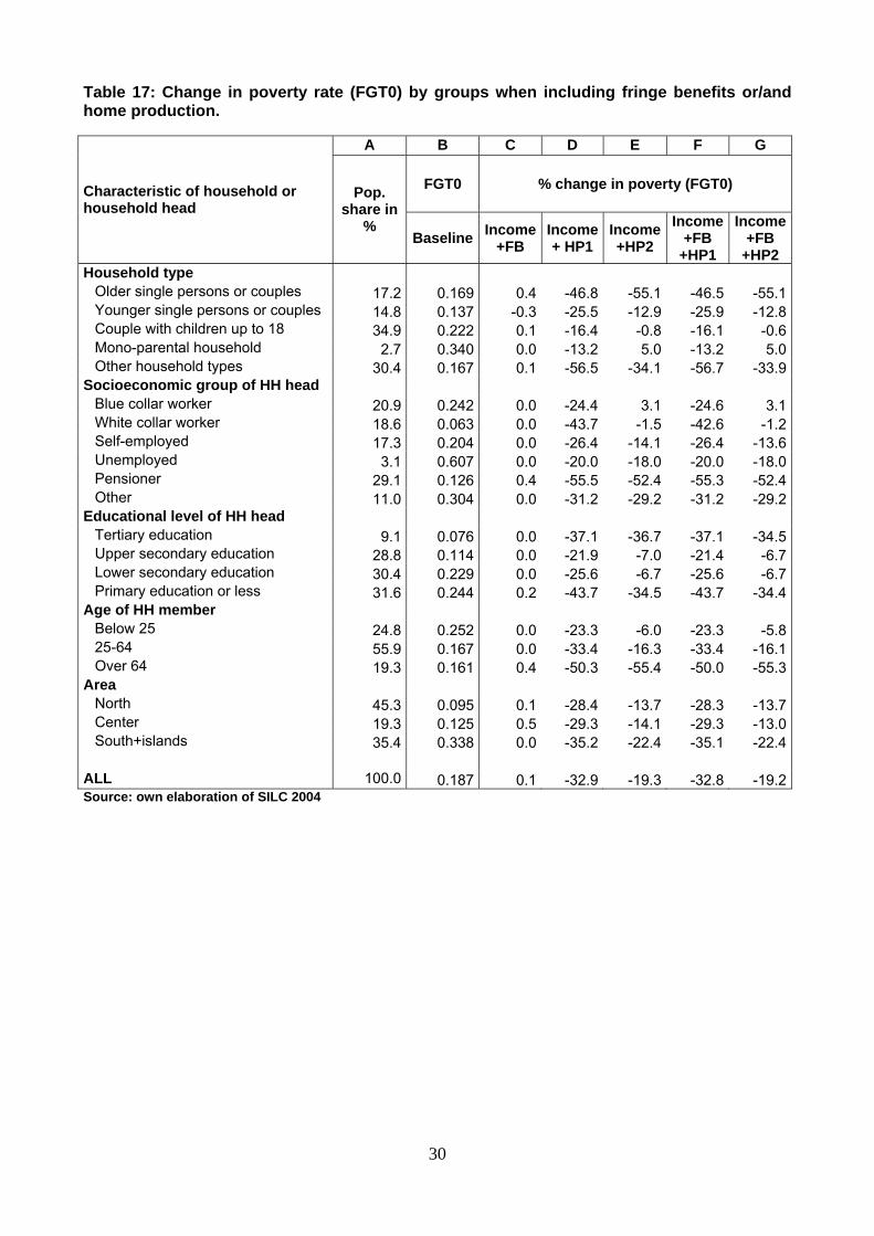
The changes in poverty are shown in Tables 17 to 19. According to both approaches, the

three poverty indices considered (FGT0, FGT1, FGT2) decreases mostly for older singles and

27

couples, for households with pensioner, with highly educated and with less educated head, for the

over64s and for the residents of South of Italy. Note, moreover, that according to the housekeeper

approach the differences in the percentage reduction of poverty are quite similar across the several

groups, while such differences appear wider with the opportunity cost approach.

Figure 7: Lorenz curves of baseline income and extended incomes

Source: own elaboration on SILC04 Figure 8: Generalized Lorenz curves of baseline income and extended incomes

Source: own elaboration on SILC04

28

Table 15: Change in income mean by groups, when including fringe benefits or/and home production.

A B C D E F G Mean % increase in mean equiv. Income

Characteristic of household or household head

Pop. share in % Baseline Income

+FB Income +HP1

Income +HP2

Income +FB+HP1

Income +FB+HP2

Household type Older single persons or couples 17.2 13914 0.0 42.5 67.9 42.5 67.9Younger single persons or couples 14.8 17507 1.0 27.1 36.4 27.9 37.1Couple with children up to 18 34.9 13819 0.9 29.9 36.3 31.1 37.2Mono-parental household 2.7 11782 2.2 32.8 36.9 34.0 37.4Other household types 30.4 15685 0.2 39.2 47.0 39.6 47.3% Within groups inequality ./. ./. ./. ./. ./. ./. ./.% Between groups inequality ./. ./. ./. ./. ./. ./. ./.

Socioeconomic group of HH head Blue collar worker 20.9 12076 0.3 38.0 40.0 38.4 40.3White collar worker 18.6 17542 2.1 25.9 34.9 28.1 36.6Self-employed 17.3 17933 0.1 26.4 32.3 26.5 32.4Unemployed 3.1 7997 1.3 60.4 70.2 61.0 70.6Pensioner 29.1 15112 0.1 40.3 58.3 40.4 58.5Other 11.0 12408 0.1 43.3 57.5 43.6 57.7% Within groups inequality ./. ./. ./. ./. ./. ./. ./.% Between groups inequality ./. ./. ./. ./. ./. ./. ./.

Educational level of HH head Tertiary education 9.1 23746 1.9 19.9 34.8 21.8 35.7Upper secondary education 28.8 16523 0.8 28.9 38.5 29.9 39.5Lower secondary education 30.4 13307 0.1 36.8 42.5 36.9 42.6Primary education or less 31.6 12394 0.1 47.0 60.4 47.1 60.5% Within groups inequality ./. ./. ./. ./. ./. ./. ./.% Between groups inequality ./. ./. ./. ./. ./. ./. ./.

Age of HH member Below 25 24.8 13292 0.8 33.8 38.8 34.7 39.425-64 55.9 15827 0.7 32.3 40.3 33.0 41.0Over 64 19.3 14249 0.1 42.5 66.5 42.6 66.6% Within groups inequality ./. ./. ./. ./. ./. ./. ./.% Between groups inequality ./. ./. ./. ./. ./. ./. ./.

Area North 45.3 17067 0.9 29.8 39.9 30.8 40.7Center 19.3 15985 0.2 32.5 43.2 32.7 43.4South+islands 35.4 11522 0.3 44.9 55.4 45.2 55.7% Within groups inequality ./. ./. ./. ./. ./. ./. ./.% Between groups inequality ./. ./. ./. ./. ./. ./. ./.

City size >50000 inhabitants 41.9 15912 1.0 32.2 43.2 32.8 43.62000-50000 inhabitants 39.5 14709 0.7 34.9 45.0 35.4 45.4<2000 inhabitants 18.6 13077 0.5 39.9 48.8 40.2 49.1% Within groups inequality ./. ./. ./. ./. ./. ./. ./.% Between groups inequality ./. ./. ./. ./. ./. ./. ./.

ALL 100.0 14895 0.6 34.5 44.8 35.1 45.4Source: own elaboration of SILC 2004

29

Table 16: Change in inequality by groups, when including fringe benefits or/and home production

A B C D E F G MLD % change in inequality Characteristic of household or

household head Pop. share in % Baseline Income+

FB Income+

HP1 Income+

HP2 Income+FB+HP1

Income+FB+HP2

Household type Older single persons or couples 17.2 0.138 0.2 -36.3 -22.2 -36.0 -22.1 Younger single persons or couples 14.8 0.208 2.0 -38.1 -26.5 -37.2 -25.6 Couple with children up to 18 34.9 0.204 2.4 -39.4 -28.2 -37.2 -26.7 Mono-parental household 2.7 0.273 6.3 -42.6 -27.2 -40.7 -26.5 Other household types 30.4 0.181 0.5 -46.7 -35.4 -46.3 -34.8 % Within groups inequality ./. 0.188 1.7 -41.0 -29.2 -39.9 -28.3 % Between groups inequality ./. 0.004 -1.6 6.5 35.8 2.4 33.0

Socioeconomic group of HH head Blue collar worker 20.9 0.133 1.4 -38.4 -17.7 -37.5 -16.9 White collar worker 18.6 0.121 7.2 -31.4 -15.1 -25.7 -11.2 Self-employed 17.3 0.292 0.2 -37.5 -31.6 -37.4 -31.4 Unemployed 3.1 0.379 2.9 -57.2 -47.4 -56.7 -47.0 Pensioner 29.1 0.129 0.4 -39.1 -26.8 -38.8 -26.3 Other 11.0 0.235 0.2 -44.9 -34.8 -44.6 -34.5 % Within groups inequality ./. 0.176 1.5 -39.6 -27.8 -38.6 -27.0 % Between groups inequality ./. 0.017 2.6 -43.3 -26.8 -42.0 -25.8

Educational level of HH head Tertiary education 9.1 0.209 2.4 -29.5 -21.7 -26.0 -20.7 Upper secondary education 28.8 0.164 1.9 -34.2 -24.2 -33.1 -22.6 Lower secondary education 30.4 0.183 0.4 -40.5 -27.0 -40.3 -26.8 Primary education or less 31.6 0.161 0.6 -43.7 -29.2 -43.6 -28.9 % Within groups inequality ./. 0.173 1.1 -38.5 -26.3 -37.7 -25.6 % Between groups inequality ./. 0.020 6.0 -52.0 -39.9 -48.6 -38.1

Age of HH member Below 25 24.8 0.215 2.1 -42.2 -30.9 -48.3 -39.0 25-64 55.9 0.196 1.7 -39.9 -28.7 -78.6 -74.7 Over 64 19.3 0.140 0.2 -37.7 -24.8 -54.6 -45.3 % Within groups inequality ./. 0.190 1.6 -40.2 -28.8 -39.1 -27.9 % Between groups inequality ./. 0.003 0.7 -19.1 43.2 -21.1 41.2

Area North 45.3 0.155 2.6 -33.8 -23.2 -31.9 -21.7 Center 19.3 0.161 0.7 -36.8 -22.9 -36.5 -22.6 South+islands 35.4 0.214 0.8 -45.3 -30.3 -44.9 -29.9 % Within groups inequality ./. 0.177 1.5 -39.3 -26.2 -38.3 -25.4 % Between groups inequality ./. 0.016 2.5 -47.5 -45.3 -45.7 -44.2

City size >50000 inhabitants 41.9 0.204 1.7 -39.2 -27.8 -38.1 -27.1 2000-50000 inhabitants 39.5 0.184 1.8 -39.8 -27.0 -38.8 -25.9 <2000 inhabitants 18.6 0.174 0.7 -41.4 -28.7 -40.7 -27.9 % Within groups inequality ./. 0.190 1.6 -39.8 -27.6 -38.8 -26.8 % Between groups inequality ./. 0.002 4.9 -48.6 -34.0 -46.7 -33.7

ALL 100.0 0.193 1.6 -39.9 -27.7 -38.9 -26.9 Source: own elaboration of SILC 2004

30

Table 17: Change in poverty rate (FGT0) by groups when including fringe benefits or/and home production.


A B C D E F G

FGT0 % change in poverty (FGT0) Characteristic of household or household head

Pop. share in

% Baseline Income

+FB Income + HP1

Income +HP2

Income+FB

+HP1

Income+FB

+HP2 Household type

Older single persons or couples 17.2 0.169 0.4 -46.8 -55.1 -46.5 -55.1Younger single persons or couples 14.8 0.137 -0.3 -25.5 -12.9 -25.9 -12.8Couple with children up to 18 34.9 0.222 0.1 -16.4 -0.8 -16.1 -0.6Mono-parental household 2.7 0.340 0.0 -13.2 5.0 -13.2 5.0Other household types 30.4 0.167 0.1 -56.5 -34.1 -56.7 -33.9

Socioeconomic group of HH head Blue collar worker 20.9 0.242 0.0 -24.4 3.1 -24.6 3.1White collar worker 18.6 0.063 0.0 -43.7 -1.5 -42.6 -1.2Self-employed 17.3 0.204 0.0 -26.4 -14.1 -26.4 -13.6Unemployed 3.1 0.607 0.0 -20.0 -18.0 -20.0 -18.0Pensioner 29.1 0.126 0.4 -55.5 -52.4 -55.3 -52.4Other 11.0 0.304 0.0 -31.2 -29.2 -31.2 -29.2

Educational level of HH head Tertiary education 9.1 0.076 0.0 -37.1 -36.7 -37.1 -34.5Upper secondary education 28.8 0.114 0.0 -21.9 -7.0 -21.4 -6.7Lower secondary education 30.4 0.229 0.0 -25.6 -6.7 -25.6 -6.7Primary education or less 31.6 0.244 0.2 -43.7 -34.5 -43.7 -34.4

Age of HH member Below 25 24.8 0.252 0.0 -23.3 -6.0 -23.3 -5.825-64 55.9 0.167 0.0 -33.4 -16.3 -33.4 -16.1Over 64 19.3 0.161 0.4 -50.3 -55.4 -50.0 -55.3

Area North 45.3 0.095 0.1 -28.4 -13.7 -28.3 -13.7Center 19.3 0.125 0.5 -29.3 -14.1 -29.3 -13.0South+islands 35.4 0.338 0.0 -35.2 -22.4 -35.1 -22.4

ALL 100.0 0.187 0.1 -32.9 -19.3 -32.8 -19.2

31

Table 18: Change in normalized poverty gap (FGT1) by groups when including fringe benefits or/and home production.

A B C D E F G

FGT1 % change in poverty (FGT1) Characteristic of household or household head

Pop. share in %

Baseline Income+FB

Income + HP1

Income +HP2

Income+FB+HP1

Income+FB+HP2

Household type Older single persons or couples 17.2 0.031 0.4 -54.1 -57.0 -53.8 -56.9Younger single persons or couples 14.8 0.046 0.1 -44.6 -27.0 -44.3 -26.9Couple with children up to 18 34.9 0.069 0.2 -37.5 -18.8 -37.3 -18.7Mono-parental household 2.7 0.130 0.1 -32.1 -10.3 -32.0 -10.2Other household types 30.4 0.051 0.2 -72.6 -58.3 -72.5 -58.2

Socioeconomic group of HH head Blue collar worker 20.9 0.064 0.2 -46.1 -10.2 -45.8 -10.1White collar worker 18.6 0.010 0.4 -50.9 -2.8 -50.8 -2.8Self-employed 17.3 0.068 0.2 -46.6 -34.0 -46.4 -33.9Unemployed 3.1 0.295 0.1 -46.2 -39.2 -46.1 -39.1Pensioner 29.1 0.025 0.4 -62.0 -63.6 -61.8 -63.5Other 11.0 0.106 0.2 -50.5 -43.5 -50.3 -43.4




ALL 100.0 0.055 0.2 -49.4 -34.0 -49.3 -33.9Source: own elaboration of SILC 2004

32

Table 19: Change in poverty (FGT2) by groups when including fringe benefits or/and home production.

A B C D E F G FGT2 % change in poverty (FGT2) Characteristic of household or

household head Pop. share in % Baseline Income

+FB Income + HP1

Income +HP2

Income+FB+HP1

Income+FB+HP2

Household type Older single persons or couples 17.2 0.011 0.4 -61.9 -61.7 -61.7 -61.6Younger single persons or couples 14.8 0.024 0.2 -57.5 -37.7 -57.3 -37.6Couple with children up to 18 34.9 0.035 0.2 -53.5 -33.7 -53.3 -33.7Mono-parental household 2.7 0.074 0.1 -45.6 -20.5 -45.4 -20.4Other household types 30.4 0.023 0.2 -81.7 -71.4 -81.6 -71.3

Socioeconomic group of HH head Blue collar worker 20.9 0.028 0.2 -61.4 -19.3 -61.2 -19.3White collar worker 18.6 0.003 0.3 -51.1 1.9 -51.1 2.2Self-employed 17.3 0.034 0.1 -61.0 -47.7 -60.8 -47.6Unemployed 3.1 0.187 0.1 -60.8 -53.3 -60.7 -53.3Pensioner 29.1 0.009 0.3 -68.1 -69.5 -67.9 -69.4Other 11.0 0.055 0.1 -60.8 -53.2 -60.6 -53.1




ALL 100.0 0.027 0.2 -61.5 -45.1 -61.3 -45.0Source: own elaboration of SILC 2004

Finally, we briefly analyze the joint effects of FB and HP on the baseline income distribution.

Looking at the Tables 10 to 19, we note that the joint effects is mainly determined by home

production, since the impact of fringe benefits is almost null. Therefore, the same comments that

we have proposed for the analysis of home production hold also for the distributional analysis of

FB and HP together.

Figures 9 and 10 show that the baseline distribution is much more unequal than the

distribution of the extended income obtained by adding both FB and HP, according both to the

housekeeper wage and to the opportunity cost approach. Moreover, with the latter approach, less

people have low-middle income and more people have higher income than with the former

approach, as confirmed also by Table 12.

33

Figure 9: Kernel estimation of the baseline income distribution (blue line) and of the extended income distribution (red line), obtained by adding fringe benefits and home production according to the “housekeeper wage” approach

Figure 10: Kernel estimation of the baseline income distribution (blue line) and of the extended income distribution (red line), obtained by adding fringe benefits and home production according to the “opportunity cost” approach

34

7. Concluding remarks

This paper has studied the effects of broadening the definition of income by taking into

account two particular types of in-kind income, i.e. the ones related to goods and services provided

either by the employer or by own (non-farm) production. We have carried out three distinct

analyses, the first one for a specific type of fringe benefits, i.e. company cars, the second one for a

wider class of fringe benefits and the third one for home production. Regarding home production, in

particular, we have performed two alternative methods on how to evaluate domestic work time.

We have shown that the incidence of fringe benefits is not very widespread in the Italian

society; however, as already underlined, information on voluntary non-wage compensation are

underestimated in the dataset that we have used (SHIW04), with the consequence that the impact

of such fringe benefits has been probably underestimated.

Our findings have shown that the addition, to the definition of income, of both company cars

alone and different fringe benefits altogether has a weak impact on the structure of the income

distribution. Inequality and poverty slightly increase for the overall population, while, when we look

at specific population subgroups, it turns out that the households with older, unemployed,

pensioner or less educated householders are the social groups that become poorer after such kind

of transfers. The groups, instead, that receive higher income after such transfers are the ones

whose within-group inequality increases more, such as the young single and couples, the

households with well-educated or high qualified head and the households in the North of Italy.

The distributional impact of home production, on the other hand, has appeared much more

relevant, independently of the approach followed. Inequality and poverty sharply reduce for the

overall population, and mostly for the subgroups of older couples and singles, for households with

pensioner or less educated head, for the over64s and for the inhabitants of small cities and of the

South of Italy. One of the main reasons of such results is that unemployed and poor people invest

more time in home production, inducing therefore to an inequality reduction.

Before concluding, we should cite some problems related to the evaluation of the

distributional impact of home production that have not been handled throughout the paper: poor

households may be forced to spend time in home production, since they cannot effort the purchase

of goods or services on the market. On the other hand, some kind of domestic works as gardening

require housing equipment, such as a garden or a terrace, thus inducing a selection of the

households. Moreover, it is difficult, from the questionnaire, to well separate the domestic work

carried out for necessity from the domestic work performed as leisure activities (such as gardening,

repairs, errands).

35

References ACI (2007), “Riferimenti normative” in www.aci.it

Agenzia delle Entrate (2007), “Reddito di lavoro dipendente, veicoli concessi in uso

promiscuo-ritenute effettuate dal sostituto sulla base delle disposizioni di cui all’art.51, comma 4,

lett. A), del Tuir”, Circolare n. 21/E

C. Biancotti, G. D’Alessio and A. Neri (2004), “Errori di misura nell’indagine sui bilanci delle

famiglie italiane”, Temi di Discussione del Servizio Studio di Banca d’Italia, n. 520

M.C. Chiavaro (2005) “I fringe benefits: analisi del trattamento fiscale dei compensi in natura

corrisposti a dipendenti e collaboratori”, available at the website

www.commercialistatelematico.com

W. Chung (2003), “Fringe benefits and inequality in the labor market”, Economic Inquiry, 41

(3), 517-529

Eurostat (2006) New income components in EU_SILC 2007 onwards: A Review. Meeting of

the Working Group “Statistics on living conditions (HBS, EU_SILC and IPSE), 15-16 May 2006,

EU-SILC DOC 165/06/EN

J. R. Frick, J. Goebel and M. Grabka (2006), “Assessing the distributional impact of “imputed

rent” and “non-cash employee income” in micro-data”, in Comparative EU statistics on Income and

Living Conditions: Issues and Challenges, Proceedings of the EU-SILC conference (Helsinki, 6-8

November 2006), €stat

Istat (2007), “L’uso del tempo. Indagine multiscopo sulle famiglie Uso del tempo Anni 2002-

2003”, ISTAT Informazioni, 2

S. P. Jenkins and N. C. O’Leary (1996), “Household income plus household production: The

distribution of extended income in the U.K.”, Review of Income and Wealth, 42 (4), 401-419

L. Gaiani (2006), “Auto aziendali: dal 2007 il reddito tassabile sale al 50%”, Il Sole 24 ore,

13/12/2006

P. Monti (2007), “Disuguaglianza di tempo”, www.lavoce.info , 24/11/2007

http://www.aci.it/

http://www.commercialistatelematico.com/

http://www.lavoce.info/

36

B. Pierce (2001), “Compensation inequality”, The Quarterly Journal of Economics, November,

1493-1525

Smeeding, T. M, Saunders, P. Coder, J., Jenkins, S., Fritzell, J., Hagenaars, A. J. M., Hauser,

R. And Wolfson, M. (1993), “Poverty, inequality, and family living standards impacts across seven

nations: The effect of noncash subsidies for health, education and housing”, Review of Income and

Wealth, 39, 3.

R. Tamburini “I fringe benefits”, da “Il Giornale del dirigente” 14(4), available on the web site

www.manageritalia.it

P. Teofilatto (2007), “Auto in fringe benefit: retromarcia sulla stangata”, Flotte e finanza,

March-April 2007, 14-19

http://www.manageritalia.it/

37

Appendix A: Econometric results

We report the econometric results obtained from the several regressions described in the paper.

Table A1 and A2 refer to the analysis of fringe benefits.

Table A1: Probit regression of the “receiving FB or not” with respect to a set of covariates. Covariates Coefficient Std. Err. z P>|z| 95% Confidence Interval

Age 0.002 0.000 29.34 0 0.001 0.163

gender -0.106 0.001 -107.2 0 -0.108 -0.104

North-West Italy 0.015 0.001 12.64 0 0.012 0.017

Center Italy -0.342 0.001 -244.86 0 -0.345 -0.339

South Italy -0.139 0.001 -93.78 0 -0.142 -0.136

Islands -0.016 0.002 -9.03 0 -0.020 -0.126

n. HH components -0.048 0.000 -118.85 0 -0.049 -0.047

education 0.112 0.000 275.92 0 0.111 0.113

log employee earned income 0.385 0.001 335.08 0 0.383 0.387

contract at will 0.046 0.002 23.68 0 0.042 0.050

constant -5.146 0.011 -489.13 0 -5.166 -5.125

Source: own elaboration of SHIW 2004

Table A2: OLS regression of the logarithmic transformation of the amount of fringe benefits (in €) with respect to a set of covariates.

Covariates Coefficient Std. Err. t P>|t| 95% Confidence Interval

Age -0.006 0.006 -0.96 0.336 -0.018 0.617

Gender -0.110 0.109 -1.01 0.312 -0.324 0.103

North West Italy 0.192 0.120 1.6 0.111 -0.044 0.428

Center Italy -0.057 0.157 -0.36 0.718 -0.366 0.253

South Italy 0.183 0.162 1.13 0.26 -0.136 0.502

Islands -0.203 0.190 -1.07 0.285 -0.575 0.170

n. HH components 0.035 0.049 0.72 0.474 -0.061 0.130

Education -0.015 0.050 -0.3 0.768 -0.112 0.831

log employee earned income 0.866 0.124 6.97 0 0.622 1.110

contract at will -0.660 0.233 -2.83 0.005 -1.118 -0.202

Constant -0.928 1.119 -0.83 0.407 -3.127 1.271

n. observation 471

adjusted R square 0.1241

Prob>F 0.000

Source: own elaboration of SHIW 2004

38

All the variables used as covariates in the probit model are significant in the determination of the

probability of receiving fringe benefit. The only two significant covariates in the OLS regression are

the logarithmic transformation of the employee income and the dummy variable “having a contract

at will or not”. Note that as the employee income increases, the amount of the fringe benefit

increases.

Tables A3 to A5 refer to the analysis of home production.

Table A3: Probit regression of “spending time in domestic work” with respect to a set of covariates

Covariates Coef. Std.Err. z P>|z| 95% Conf. Interval Age 0.002 0.000 20.15 0 0.001 0.002 Gender 0.075 0.002 42.33 0 0.072 0.079 Partner of HH head -0.114 0.002 -54.7 0 -0.118 -0.110 Son of HH head -0.085 0.003 -30.48 0 -0.091 -0.080 Parent of HH head -0.228 0.006 -41.33 0 -0.239 -0.217 Other relation with HH head -0.118 0.005 -23.83 0 -0.127 -0.108 No. HH components -0.014 0.001 -19.24 0 -0.016 -0.013 High school degree 0.081 0.002 50.8 0 0.078 0.084 University degree -0.141 0.002 -62.65 0 -0.145 -0.137 Unemployed 0.067 0.003 20.14 0 0.061 0.074 Housewife 0.026 0.002 11.57 0 0.022 0.030 Retired -0.024 0.002 -10.64 0 -0.028 -0.019 Other employment status 0.193 0.003 70.3 0 0.188 0.199 Health status -0.151 0.001 -166.84 0 -0.153 -0.149 No. of under18s 0.047 0.001 41.09 0 0.045 0.049 No. of over65s 0.087 0.001 65.5 0 0.084 0.089 No. of rooms 0.024 0.000 54.59 0 0.023 0.025 Garden -0.045 0.001 -32.82 0 -0.048 -0.043 Terrace 0.000 0.002 -0.02 0.983 -0.004 0.004 Automobile 0.004 0.002 1.64 0.101 -0.001 0.008 Constant 2.635 0.005 497.47 0 2.624 2.645


Table A3 shows that all covariates except the presence of terrace and of automobile are significant

for the probit regression.

39

Table A4: OLS regression of the logarithmic of the domestic work time with respect to a set of covariates

Covariates Coef. Std.Err. z P>|z| 95% Conf. Interval Age 0.004 0.000 9.37 0 0.003 0.005 Gender 0.041 0.009 4.37 0 0.022 0.059 Partner of HH head -0.138 0.011 -12.29 0 -0.160 -0.116 Son of HH head 0.043 0.015 2.84 0.005 0.013 0.073 Parent of HH head 0.079 0.035 2.24 0.025 0.010 0.148 Other relation with HH head -0.063 0.027 -2.34 0.019 -0.116 -0.010 No. HH components 0.009 0.004 2.13 0.033 0.001 0.016 High school degree -0.007 0.008 -0.82 0.411 -0.023 0.009 University degree -0.009 0.014 -0.68 0.496 -0.036 0.017 Unemployed 0.106 0.017 6.17 0 0.073 0.140 Housewife 0.035 0.012 2.89 0.004 0.011 0.059 Retired 0.054 0.012 4.5 0 0.030 0.077 Other employment status 0.034 0.013 2.65 0.008 0.009 0.059 Health status 0.023 0.005 4.52 0 0.013 0.032 No. Of under18s -0.027 0.006 -4.64 0 -0.038 -0.015 No. of over65s 0.007 0.007 1.01 0.314 -0.007 0.021 No. of rooms -0.002 0.002 -0.76 0.445 -0.006 0.003 Garden -0.031 0.007 -4.17 0 -0.045 -0.016 Terrace 0.014 0.011 1.32 0.186 -0.007 0.036 Automobile -0.055 0.013 -4.33 0 -0.080 -0.030 Constant 3.463 0.029 120.59 0 3.407 3.520 No. Observations 43865 Adjusted R square 0.029 Prob>F 0.000


Table A5: OLS regression of the employee earning with respect to a set of covariates for the “opportunity cost” approach

Covariates Male Female Coef. Std.Err. P>|z| Coef. Std.Err. P>|z| No. HH components 0.008 0.004 0.056 -0.003 0.006 0.595 Age 0.012 0.001 0 0.015 0.001 0 Partner of HH head 0.006 0.026 0.826 0.006 0.018 0.726 Son of HH head -0.196 0.014 0 -0.159 0.023 0 Parent of HH head -0.308 0.214 0.15 -0.131 0.136 0.334 Other relation with HH head -0.165 0.030 0 -0.073 0.040 0.07 High school degree 0.180 0.011 0 0.277 0.014 0 University degree 0.447 0.017 0 0.546 0.019 0 Good health status -0.017 0.013 0.208 -0.069 0.018 0 Quite good health status -0.084 0.016 0 -0.125 0.021 0 Bad health status -0.190 0.036 0 -0.247 0.045 0 Very bad health status -0.315 0.099 0.001 -0.165 0.106 0.119 Constatnt 1.464 0.030 0 1.216 0.038 0 No. Observations 9257 7076 Adjusted R square 0.20 0.20 Prob>F 0.00 0.00


40

Appendix B As an example, here we copy part of the tables provided by ACI (“Automobile Club d’Italia”)

for the calculation of the values of company car’s benefits for the year 2003. All the tables are

available on the website www.aci.it.

Table B1: Short extract from the ACI’s tables related to the year 2003 (automobiles with gasoline, in production)

FACTORY TYPE SERIES COST PER KM FOR

15,000 KM/YEAR (€ per Km)

ANNUAL FRINGE BENEFIT (€)

alfa romeo alfa 147 1.6/16v ts 105cv 3p.distinctive 0.4712 2,120.38 alfa romeo alfa 147 1.6/16v ts 105cv 3p.progression 0.4501 2,025.44 alfa romeo alfa 147 1.6/16v ts 105cv connect 3 p. 0.4712 2,120.38 alfa romeo alfa 147 1.6/16v ts 105cv distinctive 5p 0.4751 2,137.95 alfa romeo alfa 147 1.6/16v ts 105cv plug-in 3 p. 0.4592 2,066.25 alfa romeo alfa 147 1.6/16v ts 105cv progression 5p 0.4616 2,077.24 alfa romeo alfa 147 1.6/16v ts 120cv 3p.distinctive 0.4866 2,189.80 alfa romeo alfa 147 1.6/16v ts 120cv 3p.progression 0.4655 2,094.83 alfa romeo alfa 147 1.6/16v ts 120cv connect 3 p. 0.4835 2,175.60 alfa romeo spider 2.0/16v ts l 150cv 0.6322 2,845.11 Audi a2 1.4 75cv base 0.3961 1,782.32 Audi a2 1.4 75cv top 0.4250 1,912.42 Audi a2 1.4/16v 75cv comfort 0.4175 1,878.58 Audi a2 1.6/16v 110cv fsi base 0.4189 1,885.04 Audi a2 1.6/16v 110cv fsi comfort 0.4385 1,973.31 Audi a2 1.6/16v 110cv fsi top 0.4454 2,004.38 Audi a3 1.6 102cv attraction 0.4603 2,071.48 Audi a3 1.8 125cv attraction 0.4966 2,234.63 Audi a3 1.8 turbo 150cv attraction 0.5204 2,341.67 Audi a3 1.8 turbo 150cv attraction tiptronic 0.5373 2,417.85 Audi a3 1.8 turbo 180cv attraction 0.5405 2,432.40 Bmw 330i v6 231cv berl. 4 porte mod.2002 0.7372 3,317.61 Bmw 330xi touring v6 231 cv 5 p. sw mod.2002 0.7824 3,520.67 bmw 330xi v6 231cv berl. 4 porte mod.2002 0.7667 3,450.06 bmw 520i touring v6 170 cv chrome mod.2002 0.7673 3,452.73 bmw 520i touring v6 170 cv silver mod.2002 0.7509 3,379.18 bmw 520i touring v6 170 cv titanium mod.2002 0.7963 3,583.53 bmw 520i v6 170cv chrome berlina mod.2002 0.7397 3,328.84 bmw 520i v6 170cv silver berlina mod.2002 0.7163 3,223.28 bmw 520i v6 170cv titan. berlina mod. 2002 0.7687 3,459.24 bmw 525i touring v6 192 cv chrome mod. 2002 0.7941 3,573.40 bmw 525i touring v6 192 cv platinum mod.2002 0.8749 3,937.11 bmw 525i touring v6 192 cv silver mod.2002 0.7777 3,499.47 bmw 525i touring v6 192 cv titanium mod.2002 0.8231 3,703.78 bmw 525i v6 192cv chrome berlina mod.2002 0.7677 3,454.66 bmw 525i v6 192cv plat. berlina mod 2002 0.8485 3,818.35 Bmw 525i v6 192cv titan. berlina mod.2002 0.7967 3,585.07

http://www.aci.it/

citizens and governance in a knowledge-based society · compensation, such as leaves (vacation,...

Documents