circuit synthesis from fibonacci decision diagrams

Circuit Synthesis from Fibonacci Decision Diagrams

RADOMIR S. STANKOVICa,*, JAAKKO ASTOLAb, MILENA STANKOVICa and KAREN EGIAZARIANb

aFaculty of Electronics, Department of Computer Science, University of Nis, Beogradska 14, 18 000 Nis, Yugoslavia; bInternational Center for SignalProcessing, Tampere University of Technology, Tampere, Finland

(Received 20 January 2000; In final form 4 October 2000)

In decision diagrams (DDs) methods for circuit synthesis, it is possible to directly transfer a DD for agiven function f into a network realizing f by the replacement of non-terminal nodes in the DD with thecorresponding circuit modules.

The chief bottleneck of mapping a DD into a network is the inherent feature that the depth of thenetwork produced, is equal to the number of variables in f. For this reason, it is proposed a method forsmall depth circuit synthesis through reachability matrices describing connections among the nodes inthe DD for f.

In this paper, we first generalized DD methods for circuit design to Fibonacci interconnectiontopologies through the Fibonacci decision diagrams (FibDDs). Then, we extended the small depthcircuit synthesis method to FibDDs. In this way, design methods through DDs are completelytransferred from Boolean to Fibonacci topologies.

Keywords: Switching functions; Spectral transforms; Circuit synthesis; Fibonacci sequences;Fibonacci transforms; Decision diagrams

INTRODUCTION

The hypercube architectures and related Boolean inter-

connection topologies are extensively used in systems

design and logic design. However, in some applications,

they express some inconveniences originating in their

inherent features, as for example, restrictions to the power

of two in the number of nodes or inputs, etc. For this

reason, the generalized Fibonacci interconnection topol-

ogies are offered as an alternative [11–14,18,31].

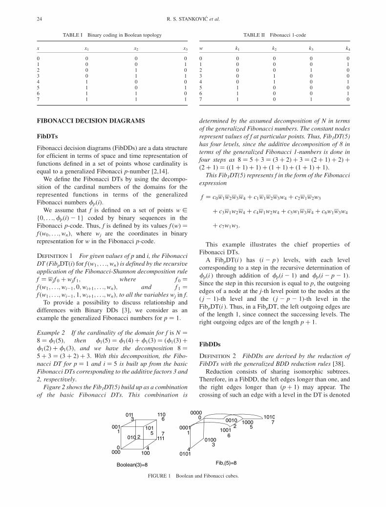
Example 1 Table I shows the coding of first eight non-

negative integers in the Boolean topology. Table II shows

the corresponding Fibonacci 1-code. Figure 1compares

the Boolean cube of order n ¼ 3; and the Fibonacci cube

of the same order derived from these codings.

There are few reasons to study the generalized

Fibonacci topologies. We want to point out the following:

1. Boolean n-cube is involved in the set of generalized

Fibonacci cubes.

2. The dimension of a generalized Fibonacci cube which

can be embeded in the Boolean n-cube with k ¼ 1; 2faulty nodes is greater than 2n21:

3. The k-th order Fibonacci cube of the dimension nþ k

is equivalent to a Boolean n-cube for 0 # n , k: It

follows that algorithms developed for a generalized

Fibonacci cube are executable on the Boolean cube of

the corresponding order.

Binary decision diagrams (BDDs) [3], and their

different generalizations [29,35,37], are a standard data

structure in many CAD systems [10] related to functions

on Boolean topologies. Fibonacci DDs (FibDDs) [39] are

extensions of DDs representations to functions on

Fibonacci topologies. Therefore, it could be interesting

to transfer design methods through different DDs in

Boolean topologies to Fibonacci DDs.

In this paper, we extend the method for circuit synthesis

through DDs [22], and Kronecker DDs [16], for switching

functions, and through Galois field DDs (GFDDs) for MV

functions [33,34], to Fibonacci DDs. We also generalized

the method for small depth circuit synthesis through the

reachability matrices [17,36] to Fibonacci DDs. Some

basic concepts about the Fibonacci numbers, codes and

related transforms are given in the Addendum.

ISSN 1065-514X print/ISSN 1563-5171 online q 2002 Taylor & Francis Ltd

DOI: 10.1080/10655140290009783

*Corresponding author.

VLSI Design, 2002 Vol. 14 (1), pp. 23–34

FIBONACCI DECISION DIAGRAMS

FibDTs

Fibonacci decision diagrams (FibDDs) are a data structure

for efficient in terms of space and time representation of

functions defined in a set of points whose cardinality is

equal to a generalized Fibonacci p-number [2,14].

We define the Fibonacci DTs by using the decompo-

sition of the cardinal numbers of the domains for the

represented functions in terms of the generalized

Fibonacci numbers fpðiÞ:We assume that f is defined on a set of points w [

{0; . . .;fpðiÞ2 1} coded by binary sequences in the

Fibonacci p-code. Thus, f is defined by its values f ðwÞ ¼

f ðw0; . . .;wnÞ; where wj are the coordinates in binary

representation for w in the Fibonacci p-code.

Definition 1 For given values of p and i, the Fibonacci

DT (FibpDT(i) for f ðw1; . . .;wnÞ is defined by the recursive

application of the Fibonacci-Shannon decomposition rule

f ¼ wjf 0 þ wjf 1; where f 0 ¼

f ðw1; . . .;wi21; 0;wiþ1; . . .;wnÞ; and f 1 ¼

f ðw1; . . .;wi21; 1;wiþ1; . . .;wnÞ; to all the variables wj in f.

To provide a possibility to discuss relationship and

differences with Binary DDs [3], we consider as an

example the generalized Fibonacci numbers for p ¼ 1:

Example 2 If the cardinality of the domain for f is N ¼

8 ¼ f1ð5Þ; then f1ð5Þ ¼ f1ð4Þ þ f1ð3Þ ¼ ðf1ð3Þ þ

f1ð2Þ þ f1ð3Þ; and we have the decomposition 8 ¼

5þ 3 ¼ ð3þ 2Þ þ 3: With this decomposition, the Fibo-

nacci DT for p ¼ 1 and i ¼ 5 is built up from the basic

Fibonacci DTs corresponding to the additive factors 3 and

2, respectively.

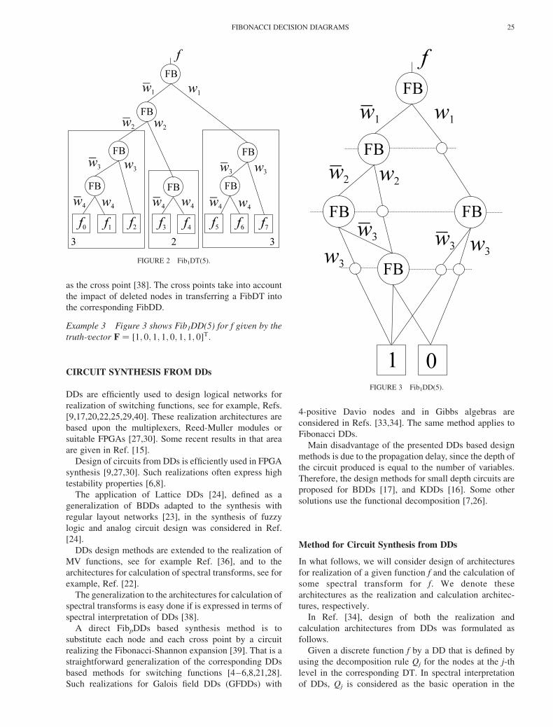
Figure 2 shows the Fib1DT(5) build up as a combination

of the basic Fibonacci DTs. This combination is

determined by the assumed decomposition of N in terms

of the generalized Fibonacci numbers. The constant nodes

represent values of f at particular points. Thus, Fib1DT(5)

has four levels, since the additive decomposition of 8 in

terms of the generalized Fibonacci 1-numbers is done in

four steps as 8 ¼ 5þ 3 ¼ ð3þ 2Þ þ 3 ¼ ð2þ 1Þ þ 2Þ þ

ð2þ 1Þ ¼ ðð1þ 1Þ þ 1Þ þ ð1þ 1Þ þ ð1þ 1Þ þ 1Þ:This Fib1DT(5) represents f in the form of the Fibonacci

expression

f ¼ c0w1w2w3w4 þ c1w1w2w3w4 þ c2w1w2w3

þ c3w1w2w4 þ c4w1w2w4 þ c5w1w3w4 þ c6w1w3w4

þ c7w1w3:

This example illustrates the chief properties of

Fibonacci DTs.

A FibpDT(i ) has (i 2 p ) levels, with each level

corresponding to a step in the recursive determination of

fp(i ) through addition of fpði 2 1Þ and fpði 2 p 2 1Þ:Since the step in this recursion is equal to p, the outgoing

edges of a node at the j-th level point to the nodes at the

( j 2 1)-th level and the ( j 2 p 2 1)-th level in the

FibpDT(i ). Thus, in a FibpDT, the left outgoing edges are

of the length 1, since connect the successing levels. The

right outgoing edges are of the length pþ 1:

FibDDs

Definition 2 FibDDs are derived by the reduction of

FibDTs with the generalized BDD reduction rules [38].

Reduction consists of sharing isomorphic subtrees.

Therefore, in a FibDD, the left edges longer than one, and

the right edges longer than ðpþ 1Þ may appear. The

crossing of such an edge with a level in the DT is denoted

TABLE I Binary coding in Boolean topology

x x1 x2 x3

0 0 0 01 0 0 12 0 1 03 0 1 14 1 0 05 1 0 16 1 1 07 1 1 1

TABLE II Fibonacci 1-code

w k1 k2 k3 k4

0 0 0 0 01 0 0 0 12 0 0 1 03 0 1 0 04 0 1 0 15 1 0 0 06 1 0 0 17 1 0 1 0

FIGURE 1 Boolean and Fibonacci cubes.

R. S. STANKOVIC et al.24

as the cross point [38]. The cross points take into account

the impact of deleted nodes in transferring a FibDT into

the corresponding FibDD.

Example 3 Figure 3 shows Fib1DD(5) for f given by the

truth-vector F ¼ ½1; 0; 1; 1; 0; 1; 1; 0�T:

CIRCUIT SYNTHESIS FROM DDs

DDs are efficiently used to design logical networks for

realization of switching functions, see for example, Refs.

[9,17,20,22,25,29,40]. These realization architectures are

based upon the multiplexers, Reed-Muller modules or

suitable FPGAs [27,30]. Some recent results in that area

are given in Ref. [15].

Design of circuits from DDs is efficiently used in FPGA

synthesis [9,27,30]. Such realizations often express high

testability properties [6,8].

The application of Lattice DDs [24], defined as a

generalization of BDDs adapted to the synthesis with

regular layout networks [23], in the synthesis of fuzzy

logic and analog circuit design was considered in Ref.

[24].

DDs design methods are extended to the realization of

MV functions, see for example Ref. [36], and to the

architectures for calculation of spectral transforms, see for

example, Ref. [22].

The generalization to the architectures for calculation of

spectral transforms is easy done if is expressed in terms of

spectral interpretation of DDs [38].

A direct FibpDDs based synthesis method is to

substitute each node and each cross point by a circuit

realizing the Fibonacci-Shannon expansion [39]. That is a

straightforward generalization of the corresponding DDs

based methods for switching functions [4–6,8,21,28].

Such realizations for Galois field DDs (GFDDs) with

4-positive Davio nodes and in Gibbs algebras are

considered in Refs. [33,34]. The same method applies to

Fibonacci DDs.

Main disadvantage of the presented DDs based design

methods is due to the propagation delay, since the depth of

the circuit produced is equal to the number of variables.

Therefore, the design methods for small depth circuits are

proposed for BDDs [17], and KDDs [16]. Some other

solutions use the functional decomposition [7,26].

Method for Circuit Synthesis from DDs

In what follows, we will consider design of architectures

for realization of a given function f and the calculation of

some spectral transform for f. We denote these

architectures as the realization and calculation architec-

tures, respectively.

In Ref. [34], design of both the realization and

calculation architectures from DDs was formulated as

follows.

Given a discrete function f by a DD that is defined by

using the decomposition rule Qj for the nodes at the j-th

level in the corresponding DT. In spectral interpretation

of DDs, Qj is considered as the basic operation in the

FIGURE 2 Fib1DT(5).

FIGURE 3 Fib1DD(5).

FIBONACCI DECISION DIAGRAMS 25

FFT-like algorithm for a spectral transform Q used to

assign f to the DT.

1. To realize f, assign a module Q performing the

operation inverse to Qj to each node and the cross

point in the DD for f.

2. To calculate the Q-spectrum for f, assign a multi-

plexer-like module to each node and the cross point in

the DD for f.

Note that in FibDTs, the same as in BDTs and

MTBDTs, we use the identical mapping to assign f to the

DT. The identical mapping is a self-inverse mapping. It

follows that the architectures for realization of f and the

calculation of the corresponding Fibonacci p-spectra for f

can be designed from the FibDDs for f in the following

way.

1. To realize f, assign a multiplexer-like module to each

node in the FibDT for f.

2. To calculate the Fibonacci p-spectrum for f, assign to

each node and the cross point in the FibDT for f a

module realizing the basic operation used in

calculation of this transform through DDs using the

top-down strategy.

The method will be explained and illustrated by the

examples of architectures for realization of a given f

defined in f1ð5Þ points and for the calculation of the

FWHT and the Fibonacci-Haar spectra of order f1ð5Þ:

Architecture for Realization of f

In the FibDD for a given f, the constant nodes shows the

values f ðwÞ; w [ {0; . . .;fpðiÞ2 1}; for f at particular

points of the domain of definition for f. These points are

denoted by binary sequences in the Fibonacci p-code. The

FibDD consists of nodes with two outgoing edges.

Therefore, to design an architecture which realizes f, it is

enough to assign a ð2 £ 1Þ multiplexer to each node in the

FibDD for f.

The sequence kðwÞ ¼ {k1; . . .; ki2p} of the values of

control inputs for the multiplexers at the moment w is

equal to the code word w in the Fibonacci p-code. The

following example illustrates the design of a realization

architecture for a given f derived from the FibDTs. The

same method applies to the FibDDs, since the reduction of

a DT into a DD by the generalized BDD reduction rules

[38] does not destroy nor diminish the information content

of a DT. If the design is based on the FibDD for f, some

multiplexers can be saved, since the number of nodes is

reduced. However, these savings depend on the peculiar

properties of f permitting reduction of the FibDT into the

FibDD for f.

Example 4 Figure 4 shows the architecture for the

realization of functions represented by the Fib1DT(5).

Table II shows the values of control inputs for the

multiplexers.

Example 5 Figure 5 shows a realization for f in Example

3 from the Fib1DD(5) in Fig. 3, assuming that the

multiplexer-like modules FibS realizing the Fibonacci-

Shannon expansion are provided.

Calculation Architecture for FWHT

The FW1HT is calculated through FibDDs by using the

basic transform matrix [14]

FW ¼

1 0ffiffiffi2p

0ffiffiffi2p

0

1 0 2ffiffiffi2p

26643775:

For the design purposes, we transfer this matrix into a

FIGURE 4 Architecture for realization of f represented by the Fib1DT(5).


matrix

FWr ¼

1 0 1

0ffiffiffi2p

0

1 0 21

26643775:

The remaining multiplications byffiffiffi2p

are realized as the

multiplications at the input connections. The network

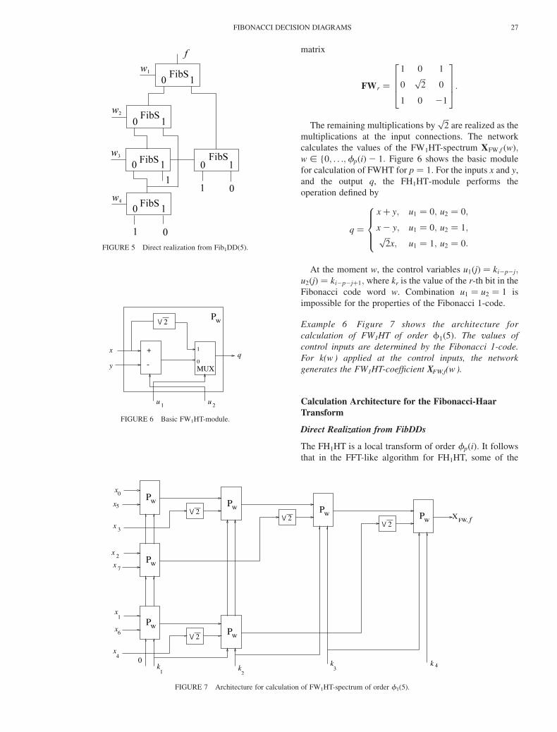
calculates the values of the FW1HT-spectrum XFW;f ðwÞ;w [ {0; . . .;fpðiÞ2 1: Figure 6 shows the basic module

for calculation of FWHT for p ¼ 1: For the inputs x and y,

and the output q, the FH1HT-module performs the

operation defined by

q ¼

xþ y; u1 ¼ 0; u2 ¼ 0;

x 2 y; u1 ¼ 0; u2 ¼ 1;ffiffiffi2p

x; u1 ¼ 1; u2 ¼ 0:

8>><>>:At the moment w, the control variables u1ðjÞ ¼ ki2p2j;

u2ðjÞ ¼ ki2p2jþ1; where kr is the value of the r-th bit in the

Fibonacci code word w. Combination u1 ¼ u2 ¼ 1 is

impossible for the properties of the Fibonacci 1-code.

Example 6 Figure 7 shows the architecture for

calculation of FW1HT of order f1ð5Þ: The values of

control inputs are determined by the Fibonacci 1-code.

For k(w ) applied at the control inputs, the network

generates the FW1HT-coefficient XFW,f(w ).

Calculation Architecture for the Fibonacci-Haar

Transform

Direct Realization from FibDDs

The FH1HT is a local transform of order fpðiÞ: It follows

that in the FFT-like algorithm for FH1HT, some of the

FIGURE 6 Basic FW1HT-module.

FIGURE 7 Architecture for calculation of FW1HT-spectrum of order f1(5).

FIGURE 5 Direct realization from Fib1DD(5).


FH1HT-spectral coefficients are calculated up to a

multiplicative constant in k steps, 1 # k # ði 2 pÞ:These coefficients are forwarded from the k-th step to

the output of the algorithm multiplied byffiffiffi2p

in each step.

In calculation through FibDDs, this property implies that

these coefficients are determined by processing of nodes at

the k-th level in the FibDD. To get their final values, these

coefficients should be multiplied by a weighting

coefficient zk ¼ ðffiffiffi2pÞk21; k ¼ 1; . . .i 2 p; This property

requires a modification in the basic FH1HT-module,

compared to the FW1HT-module. The basic FH1HT-

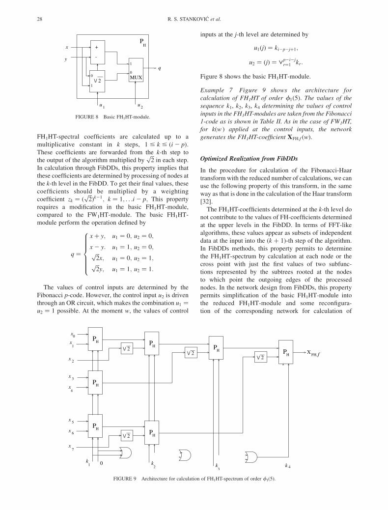
module perform the operation defined by

q ¼

xþ y; u1 ¼ 0; u2 ¼ 0;

x 2 y: u1 ¼ 1; u2 ¼ 0;ffiffiffi2p

x; u1 ¼ 0; u2 ¼ 1;ffiffiffi2p

y; u1 ¼ 1; u2 ¼ 1:

8>>>>><>>>>>:The values of control inputs are determined by the

Fibonacci p-code. However, the control input u2 is driven

through an OR circuit, which makes the combination u1 ¼

u2 ¼ 1 possible. At the moment w, the values of control

inputs at the j-th level are determined by

u1ðjÞ ¼ ki2p2jþ1;

u2 ¼ ðjÞ ¼ _p2i2jr¼1 kr:

Figure 8 shows the basic FH1HT-module.


calculation of FH1HT of order f1ð5Þ: The values of the

sequence k1, k2, k3, k4 determining the values of control

inputs in the FH1HT-modules are taken from the Fibonacci

1-code as is shown in Table II. As in the case of FW1HT,

for k(w ) applied at the control inputs, the network

generates the FH1HT-coefficient XFH;f ðwÞ.

Optimized Realization from FibDDs

In the procedure for calculation of the Fibonacci-Haar

transform with the reduced number of calculations, we can

use the following property of this transform, in the same

way as that is done in the calculation of the Haar transform

[32].

The FH1HT-coefficients determined at the k-th level do

not contribute to the values of FH-coefficients determined

at the upper levels in the FibDD. In terms of FFT-like

algorithms, these values appear as subsets of independent

data at the input into the (k þ 1)-th step of the algorithm.

In FibDDs methods, this property permits to determine

the FH1HT-spectrum by calculation at each node or the

cross point with just the first values of two subfunc-

tions represented by the subtrees rooted at the nodes

to which point the outgoing edges of the processed

nodes. In the network design from FibDDs, this property

permits simplification of the basic FH1HT-module into

the reduced FH1HT-module and some reconfigura-

tion of the corresponding network for calculation of

FIGURE 8 Basic FH1HT-module.

FIGURE 9 Architecture for calculation of FH1HT-spectrum of order f1(5).


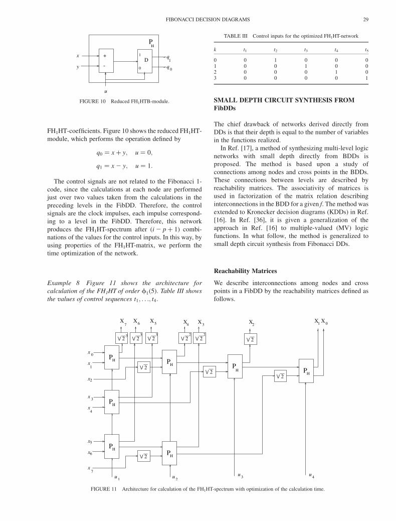
FH1HT-coefficients. Figure 10 shows the reduced FH1HT-

module, which performs the operation defined by

q0 ¼ xþ y; u ¼ 0;

q1 ¼ x 2 y; u ¼ 1:

The control signals are not related to the Fibonacci 1-

code, since the calculations at each node are performed

just over two values taken from the calculations in the

preceding levels in the FibDD. Therefore, the control

signals are the clock impulses, each impulse correspond-

ing to a level in the FibDD. Therefore, this network

produces the FH1HT-spectrum after ði 2 pþ 1Þ combi-

nations of the values for the control inputs. In this way, by

using properties of the FH1HT-matrix, we perform the

time optimization of the network.


calculation of the FH1HT of order f1ð5Þ: Table III shows

the values of control sequences t1; . . .; t4:

SMALL DEPTH CIRCUIT SYNTHESIS FROM

FibDDs

The chief drawback of networks derived directly from

DDs is that their depth is equal to the number of variables

in the functions realized.

In Ref. [17], a method of synthesizing multi-level logic

networks with small depth directly from BDDs is

proposed. The method is based upon a study of

connections among nodes and cross points in the BDDs.

These connections between levels are described by

reachability matrices. The associativity of matrices is

used in factorization of the matrix relation describing

interconnections in the BDD for a given f. The method was

extended to Kronecker decision diagrams (KDDs) in Ref.

[16]. In Ref. [36], it is given a generalization of the

approach in Ref. [16] to multiple-valued (MV) logic

functions. In what follow, the method is generalized to

small depth circuit synthesis from Fibonacci DDs.

Reachability Matrices

We describe interconnections among nodes and cross

points in a FibDD by the reachability matrices defined as

follows.

FIGURE 10 Reduced FH1HTB-module.

FIGURE 11 Architecture for calculation of the FH1HT-spectrum with optimization of the calculation time.

TABLE III Control inputs for the optimized FH1HT-network

k t1 t2 t3 t4 t5

0 0 1 0 0 01 0 0 1 0 02 0 0 0 1 03 0 0 0 0 1


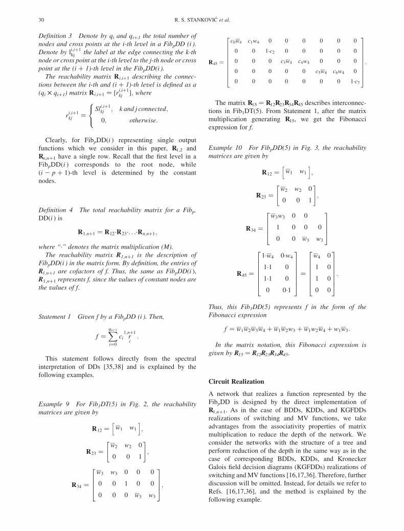
Definition 3 Denote by qi and qiþ1 the total number of

nodes and cross points at the i-th level in a FibpDD (i ).

Denote by li;iþ1kj the label at the edge connecting the k-th

node or cross point at the i-th level to the j-th node or cross

point at the (i þ 1)-th level in the FibpDD(i ).

The reachability matrix Ri;iþ1 describing the connec-

tions between the i-th and (i þ 1)-th level is defined as a

(qi £ qiþ1) matrix Ri;iþ1 ¼ ½ri;iþ1kj �; where

ri;iþ1kj ¼

Sli;iþ1kj ; k and j connected;

0; otherwise:

8<:Clearly, for FibpDD(i ) representing single output

functions which we consider in this paper, R1,2 and

Rn,nþ1 have a single row. Recall that the first level in a

FibpDD(i ) corresponds to the root node, while

(i 2 p þ 1)-th level is determined by the constant

nodes.

Definition 4 The total reachability matrix for a Fibp-

DD(i ) is

R1;nþ1 ¼ R12·R23·. . .·Rn;nþ1;

where “·” denotes the matrix multiplication (M).

The reachability matrix R1,nþ1 is the description of

FibpDD(i ) in the matrix form. By definition, the entries of

R1,nþ1 are cofactors of f. Thus, the same as FibpDD(i ),

R1,nþ1 represents f, since the values of constant nodes are

the values of f.

Statement 1 Given f by a FibpDD (i ). Then,

f ¼Xqnþ1

i¼0

ci r1;nþ1

i:

This statement follows directly from the spectral

interpretation of DDs [35,38] and is explained by the

following examples.

Example 9 For Fib1DT(5) in Fig. 2, the reachability

matrices are given by

R12 ¼ w1 w1

h i;

R23 ¼w2 w2 0

0 0 1

" #;

R34 ¼

w3 w3 0 0 0

0 0 1 0 0

0 0 0 w3 w3

26643775;

R45 ¼

c0w4 c1w4 0 0 0 0 0 0

0 0 1·c2 0 0 0 0 0

0 0 0 c3w4 c4w4 0 0 0

0 0 0 0 0 c5w4 c6w4 0

0 0 0 0 0 0 0 1·c7

2666666664

3777777775:

The matrix R15 ¼ R12R23R34R45 describes interconnec-

tions in Fib1DT(5). From Statement 1, after the matrix

multiplication generating R15, we get the Fibonacci

expression for f.

Example 10 For FibpDD(5) in Fig. 3, the reachability

matrices are given by

R12 ¼ w1 w1

h i;

R23 ¼w2 w2 0

0 0 1

" #;

R34 ¼

w3w3 0 0

1 0 0 0

0 0 w3 w3

26643775

R45 ¼

1·w4 0·w4

1·1 0

1·1 0

0 0·1

2666664

3777775 ¼w4 0

1 0

1 0

0 0

2666664

3777775:

Thus, this Fib1DD(5) represents f in the form of the

Fibonacci expression

f ¼ w1w2w3w4 þ w1w2w3 þ w1w2w4 þ w1w3:

In the matrix notation, this Fibonacci expression is

given by R15 ¼ R12R23R34R45.

Circuit Realization

A network that realizes a function represented by the

FibpDD is designed by the direct implementation of

R1,nþ1. As in the case of BDDs, KDDs, and KGFDDs

realizations of switching and MV functions, we take

advantages from the associativity properties of matrix

multiplication to reduce the depth of the network. We

consider the networks with the structure of a tree and

perform reduction of the depth in the same way as in the

case of corresponding BDDs, KDDs, and Kronecker

Galois field decision diagrams (KGFDDs) realizations of

switching and MV functions [16,17,36]. Therefore, further

discussion will be omitted. Instead, for details we refer to

Refs. [16,17,36], and the method is explained by the

following example.


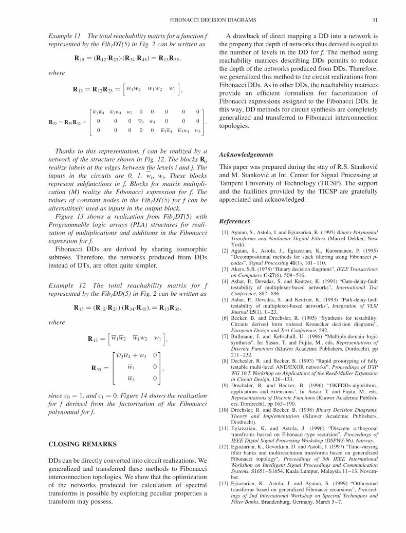
Example 11 The total reachability matrix for a function f

represented by the Fib1DT(5) in Fig. 2 can be written as

R15 ¼ ðR12·R23Þ·ðR34·R45Þ ¼ R13R35;

where

R13 ¼ R12R23 ¼ w1w2 w1w2 w1

h i;

R35 ¼ R34R45 ¼

w3w4 w3w4 w3 0 0 0 0 0

0 0 0 w4 w4 0 0 0

0 0 0 0 0 w3w4 w3w4 w3

26643775:

Thanks to this representation, f can be realized by a

network of the structure shown in Fig. 12. The blocks Rij

realize labels at the edges between the levels i and j. The

inputs in the circuits are 0, 1, wi, wi. These blocks

represent subfunctions in f. Blocks for matrix multipli-

cation (M) realize the Fibonacci expression for f. The

values of constant nodes in the Fib1DT(5) for f can be

alternatively used as inputs in the output block.

Figure 13 shows a realization from Fib1DT(5) with

Programmable logic arrays (PLA) structures for reali-

zation of multiplications and additions in the Fibonacci

expression for f.

Fibonacci DDs are derived by sharing isomorphic

subtrees. Therefore, the networks produced from DDs

instead of DTs, are often quite simpler.

Example 12 The total reachability matrix for f

represented by the Fib1DD(5) in Fig. 2 can be written as

R15 ¼ ðR12·R23Þ·ðR34·R45Þ;¼ R13R35;

where

R13 ¼ w1w2 w1w2 w1

h i;

R35 ¼

w3w4 þ w3 0

w4 0

w3 0

26643775;

since c0 ¼ 1; and c1 ¼ 0: Figure 14 shows the realization

for f derived from the factorization of the Fibonacci

polynomial for f.

CLOSING REMARKS

DDs can be directly converted into circuit realizations. We

generalized and transferred these methods to Fibonacci

interconnection topologies. We show that the optimization

of the networks produced for calculation of spectral

transforms is possible by exploiting peculiar properties a

transform may possess.

A drawback of direct mapping a DD into a network is

the property that depth of networks thus derived is equal to

the number of levels in the DD for f. The method using

reachability matrices describing DDs permits to reduce

the depth of the networks produced from DDs. Therefore,

we generalized this method to the circuit realizations from

Fibonacci DDs. As in other DDs, the reachability matrices

provide an efficient formalism for factorization of

Fibonacci expressions assigned to the Fibonacci DDs. In

this way, DD methods for circuit synthesis are completely

generalized and transferred to Fibonacci interconnection

topologies.

Acknowledgements

This paper was prepared during the stay of R.S. Stankovic

and M. Stankovic at Int. Center for Signal Processing at

Tampere University of Technology (TICSP). The support

and the facilities provided by the TICSP are gratefully

appreciated and acknowledged.

References

[1] Agaian, S., Astola, J. and Egiazarian, K. (1995) Binary PolynomialTransforms and Nonlinear Digital Filters (Marcel Dekker, NewYork).

[2] Agaian, S., Astola, J., Egiazarian, K., Kuosmanen, P. (1995)“Decompositional methods for stack filtering using Fibonacci p-codes”, Signal Processing 41(1), 101–110.

[3] Akers, S.B. (1978) “Binary decision diagrams”, IEEE Transactionson Computers C-27(6), 509–516.

[4] Ashar, P., Devadas, S. and Keutzer, K. (1991) “Gate-delay-faulttestability of multiplexer-based networks”, International TestConference, 887–896.

[5] Ashar, P., Devadas, S. and Keutzer, K. (1993) “Path-delay-faulttestability of multiplexer-based networks”, Integration of VLSIJournal 15(1), 1–23.

[6] Becker, B. and Drechsler, R. (1995) “Synthesis for testability:Circuits derived form ordered Kronecker decision diagrams”,European Design and Test Conference, 592.

[7] Bullmann, J. and Kebschull, U. (1996) “Multiple-domain logicsynthesis”, In: Sasao, T. and Fujita, M., eds, Representations ofDiscrete Functions (Kluwer Academic Publishers, Dordrecht), pp211–232.

[8] Dechesler, R. and Becker, B. (1993) “Rapid prototyping of fullytestable multi-level AND/EXOR networks”, Proceedings of IFIPWG 10.5 Workshop on Applications of the Reed-Muller Expansionin Circuit Design, 126–133.

[9] Drechsler, R. and Becker, B. (1996) “OKFDDs-algorithms,applications and extensions”, In: Sasao, T. and Fujita, M., eds,Representations of Discrete Functions (Kluwer Academic Publish-ers, Dordrecht), pp 163–190.

[10] Drechsler, R. and Becker, B. (1998) Binary Decision Diagrams,Theory and Implementation (Kluwer Academic Publishers,Dordrecht).

[11] Egiazarian, K. and Astola, J. (1996) “Discrete orthogonaltransforms bassed on Fibonacci-type recursion”, Proceedings ofIEEE Digtal Signal Processing Workshop (DSPWS-96), Norway.

[12] Egiazarian, K., Gevorkian, D. and Astola, J. (1997) “Time-varyingfilter banks and multiresolution transforms based on generalizedFibonacci topology”, Proceedings of 5th IEEE InternationalWorkshop on Intelligent Signal Proceedings and CommunicationSystems, S1651–S1654, Kuala Lumpur, Malaysia 11–13, Novem-ber.

[13] Egiazarian, K., Astola, J. and Agaian, S. (1999) “Orthogonaltransforms based on generalized Fibonacci recursions”, Proceed-ings of 2nd International Workshop on Spectral Techniques andFilter Banks, Brandenburg, Germany, March 5–7.


[14] Egiazarian, K. and Astola, J. (1997) “On generalized Fibonaccicubes and unitary transforms”, Applicable Algebra in Engineering,Communication and Computing AAECC 8, 371–377.

[15] H.Md., Hasan Babu and Sasao, T. (1998) “Design of multiple-output networks using time domain multiplexing and shared multi-terminal multiple-valued decision diagrams”, Proceedings of 28thInternational Symposium on Multiple-Valued Logic, Fukuoka,Japan, May 27–29.

[16] Hengster, H., Drechsler, R., Eckrich, S., Pfeiffer, T. and Becker, B.(1996) “AND/EXOR based synthesis of testable KFDD-circuitswith small depth”, Proceedings of Asian Test Symposium.

[17] Ishiura, N. (1992) “Synthesis of multi-level logic circuits formbinary decision diagrams”, SASIMI, 74–83.

[18] Jiang, F.-S., Horng, S.-J. and Kao, T.-W. (1997) “Embeding ofgeneralized Fibonacci cubes in hypercubes with faulty nodes”,IEEE Transactions on Parallel and Distributed Systems 8(7),727–737.

[19] Karpovsky, M.G. (1976) Finite Orthogonal Series in the Design ofDigital Devices (Wiley and JUP, New York and Jerusalem).

[20] Kebschull, U., Schubert, E. and Rosenstiel, W. (1992) “Multilevellogic synthesis based on functional decision diagrams”, EuropeanConference on Design Automation, 43–47.

[21] Le, V.V, Besson, T., Abbara, A., Brasen, D., Bogushevitsh, H.,Saucier, G. and Crastes, M. (1995) “ASIC prototyping with areaoriented mapping for ALTERA/FLEX devices”, SASIMI, 176–183.

[22] McKenzie, L., Xu, L. and Almaini, A. (1993) “Graphicalrepresentations of generalized Reed-Muller Expansions”, In:Kebschull, U., Schubert, E. and Rosenstiel, W., eds, Proceedingsof IFIP WG 10.5 Workshop on Applications of the Reed-MullerExpansion in Circuit Design, September 16–17, Hamburg,Germany, pp 181–187.

[23] Perkowski, M.A., Jozwiak, L. and Drechsler, R. (1997) “Newhierarchies of AND/EXOR trees, decision diagrams, latticediagrams, canonical forms, and regular layouts”, Proceedings ofIFIP WG 10.5 Workshop on Applications of the Reed-MullerExpansion in Circuit Design Reed-Muller ’97, 115–132, Oxford,England.

[24] Perkowski, M.A., Pierzchala, E. and Drechsler, R. (1997) “Ternaryand quaternary lattice diagrams for linearly-independent logic,multiple-valued logic, and analog synthesis”, Proceedings ofInternational Conference on Information, Communication andSignal Processing, ICICS ’97, 269–273, Singapore, September 9–12.

[25] Sarabi, A., Ho, P.F., Iravani, K., Daasch, W.R. and Perkowski, M.A.(1993) “Minimal multi-level realization of switching functionsbased on Kronecker functional decision diagrams”, Proceedings ofInternational Workshop on Logic Synthesis, 3a1–3a6, Lake Tahoe,CA, USA.

[26] Sasao, T. (1993) “FPGA design by generalized functionaldecomposition”, In: Sasao, T., ed, Logic Synthesis and Optimization(Kluwer Academic Publishers, Dordrecht), pp 233–258.

[27] Sasao, T. and Butler, J.T. (1994) “A design method for look-up tabletype FPGA by pseudo-Kronecker expansions”, Proceedings of 24thInternational Symposium on Multiple-Valued Logic, 97–106,Boston, Massachusetts, May 25–27.

[28] Sasao, T., Hamachi, H., Wado, S. and Matsuura, M. (1995) “Multi-level logic synthesis based on pseudo-Kronecker decision diagramsand local trasnformation”, Proceedings of IFIP WG 10.5 Workshopon Applications of the Reed-Muller Expansion in Circuit Design,Reed-Muller ’95, 152–160.

[29] Sasao, T. and Fujita, M. (eds) (1996) In: Representations of DiscreteFunctions (Kluwer Academic Publishers, Dordrecht).

[30] Schaefer, I., Perkowski, M.A. and Wu, H. (1993) “Multilevel logicsynthesis for cellular FPGAs based on orthogonal expansions”, In:Kebschull, U., Schubert, E. and Rosenstiel, W., eds, Proceedings ofIFIP WG 10.5 Workshop on Applications of the Reed-MullerExpansion in Circuit Design, September 17–19, Hamburg,Germany, pp 42–51.

[31] Stakhov, A.P. (1979) Algorithmic Measurement Theory (Znanie,Moscow), No. 6, 64 p, in Russian.

[32] Stankovic, M., Jankovic, D. and Stankovic, R.S. (1996) “Efficientalgorithms for Haar spectrum calculation”, Scientific Review 21–22, 171–182.

[33] Stankovic, R.S. (1995) “Functional decision diagrams for multiple-valued functions”, Proceedings of 25-th International Symposiumon Multiple-Valued Logic, 284–289.

[34] Stankovic, R.S. (1997) “Functional decision diagrams for multiple-valued functions”, Multiple-Valued Logic Journal.

[35] Stankovic, R.S. (1998) Spectral Tansform Decision Diagrams inSimple Questions and Simple Answers (Nauka, Belgrade).

[36] Stankovic, R.S. and Drechsler, R. (1997) “Circuit design fromKronecker Galois field decision diagrams for multiple-valued logicfunctions”, Proceedings of IEEE International Symposium onMultiple-Valued Logic, 275–280, Antigonish, Nova Scotia,Canada.

[37] Stankovic, R.S. and Sasao, T. (1998) “Decision diagrams forrepresentation of discrete functions: uniform interpretation andclassification”, Proceedings of ASP-DAC ’98, Yokohama, Japan,February 13–17.

[38] Stankovic, R.S., Sasao, T., Moraga, C. “Spectral transform decisiondiagrams”, in: [29], 55–92.

[39] Stankovic, M., Stankovic, R.S., Astola, J.T. and Egiazarian, K.(2000) “Fibonacci decision diagrams and spectral transformFibonacci decision diagrams”, Proceedings of 30th InternationalSymposium on Multiple-Valued Logic, Portland, Oregon, USA, May23–26.

[40] Wu, H., Perkowski, M.A. and Zhuang, N. (1993) “Synthesis ofmultiplexer directed-acyclic-graph network with application toFPGA and BDDs”, Proceedings of International Workshop onLogic Synthesis, Tahoe City, USA, May 23–26, 8d/1–8.

ADDENDUM

Fibonacci p-numbers

Definition 5 A sequence f(n ) is the Fibonacci sequence

if for each n $ 1;

fðnÞ ¼ fðn 2 1Þ þ fðn 2 2Þ;

with initial values fð0Þ ¼ 1; fðnÞ ¼ 0; n , 0: Elements of

this sequence are the Fibonacci numbers.

A generalization of Fibonacci numbers is given in Refs.

[13,31] as follows.

Definition 6 A sequence fpðiÞ is the generalized

Fibonacci p-sequence if

fpðiÞ ¼

0; i , 0;

1; i ¼ 0;

fpði 2 1Þ þ fpði 2 p 2 1Þ; i . 0:

8>><>>:Elements of this sequence are the generalized Fibonacci

p-numbers.

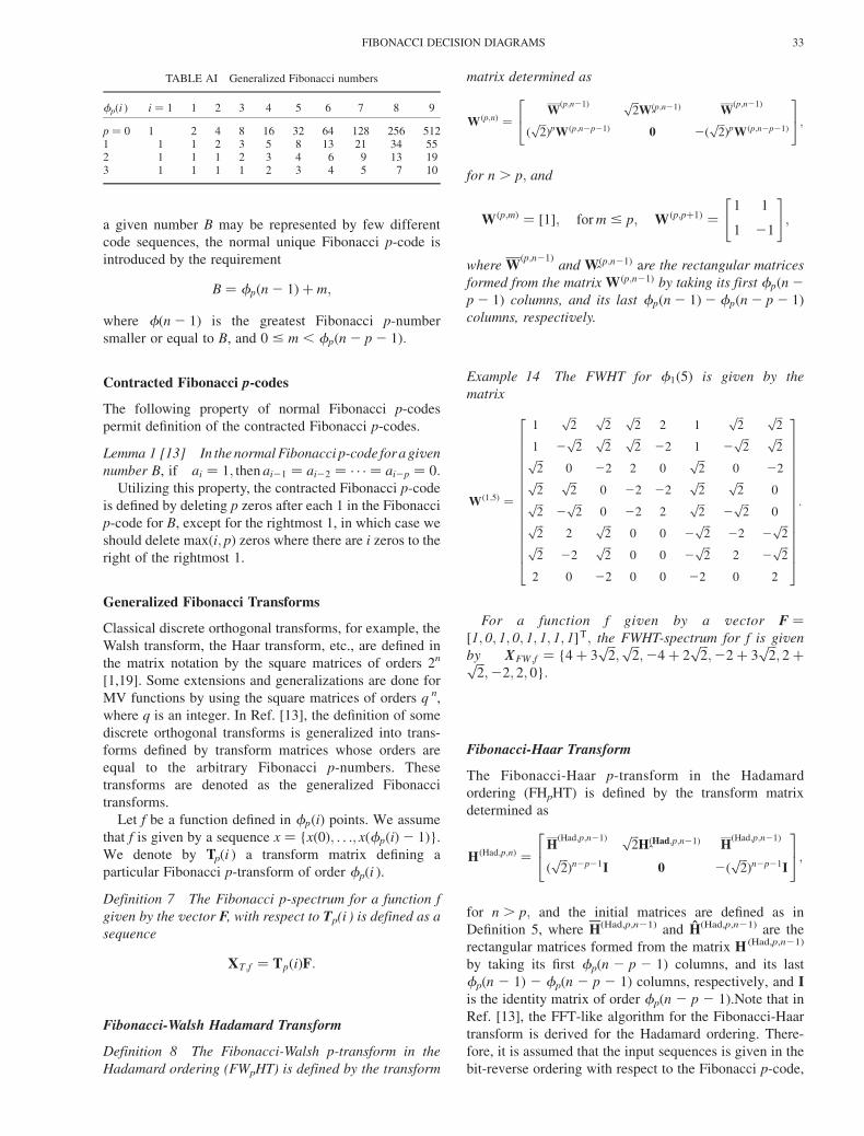
Example 13 Table AI shows the generalized Fibonacci

p-numbers for p ¼ 0, 1, 2, and 3, and i ¼ 0; 1; . . .; 9:

Fibonacci p-codes

The Fibonacci p-representation of a natural number B is

defined as

B ¼Xn21

i¼p

aifpðiÞ:

The sequence a ¼ (an21,. . .,ap)p is the Fibonacci p-code

for B [13]. Since with thus defined weighting coefficients,


a given number B may be represented by few different

code sequences, the normal unique Fibonacci p-code is

introduced by the requirement

B ¼ fpðn 2 1Þ þ m;

where fðn 2 1Þ is the greatest Fibonacci p-number

smaller or equal to B, and 0 # m , fpðn 2 p 2 1Þ:

Contracted Fibonacci p-codes

The following property of normal Fibonacci p-codes

permit definition of the contracted Fibonacci p-codes.

Lemma 1 [13] In the normal Fibonacci p-code for a given

number B, if ai ¼ 1; then ai21 ¼ ai22 ¼ · · · ¼ ai2p ¼ 0:Utilizing this property, the contracted Fibonacci p-code

is defined by deleting p zeros after each 1 in the Fibonacci

p-code for B, except for the rightmost 1, in which case we

should delete maxði; pÞ zeros where there are i zeros to the

right of the rightmost 1.

Generalized Fibonacci Transforms

Classical discrete orthogonal transforms, for example, the

Walsh transform, the Haar transform, etc., are defined in

the matrix notation by the square matrices of orders 2n

[1,19]. Some extensions and generalizations are done for

MV functions by using the square matrices of orders q n,

where q is an integer. In Ref. [13], the definition of some

discrete orthogonal transforms is generalized into trans-

forms defined by transform matrices whose orders are

equal to the arbitrary Fibonacci p-numbers. These

transforms are denoted as the generalized Fibonacci

transforms.

Let f be a function defined in fpðiÞ points. We assume

that f is given by a sequence x ¼ {xð0Þ; . . .; xðfpðiÞ2 1Þ}.

We denote by Tp(i ) a transform matrix defining a

particular Fibonacci p-transform of order fp(i ).

Definition 7 The Fibonacci p-spectrum for a function f

given by the vector F, with respect to Tp(i ) is defined as a

sequence

XT ;f ¼ TpðiÞF:

Fibonacci-Walsh Hadamard Transform

Definition 8 The Fibonacci-Walsh p-transform in the

Hadamard ordering (FWpHT) is defined by the transform

matrix determined as

Wðp;nÞ ¼Wðp;n21Þ ffiffiffi

2p

W^ðp;n21Þ W

ðp;n21Þ

ðffiffiffi2pÞpWðp;n2p21Þ 0 2ð

ffiffiffi2pÞpWðp;n2p21Þ

24 35;for n . p; and

Wðp;mÞ ¼ ½1�; for m # p; Wðp;pþ1Þ ¼1 1

1 21

" #;

where Wðp;n21Þ

and Wðp;n21Þ are the rectangular matrices

formed from the matrix Wðp;n21Þ by taking its first fpðn 2

p 2 1Þ columns, and its last fpðn 2 1Þ2 fpðn 2 p 2 1Þ

columns, respectively.

Example 14 The FWHT for f1ð5Þ is given by the

matrix

Wð1;5Þ ¼

1ffiffiffi2p ffiffiffi

2p ffiffiffi

2p

2 1ffiffiffi2p ffiffiffi

2p


2p ffiffiffi

2p

22 1 2ffiffiffi2p ffiffiffi

2pffiffiffi

2p

0 22 2 0ffiffiffi2p


2p


2p

0ffiffiffi2p

2ffiffiffi2p

0 22 2ffiffiffi2p

2ffiffiffi2p

0ffiffiffi2p

2ffiffiffi2p

0 0 2ffiffiffi2p

22 2ffiffiffi2pffiffiffi

2p

22ffiffiffi2p

0 0 2ffiffiffi2p

2 2ffiffiffi2p

2 0 22 0 0 22 0 2

266666666666666664

377777777777777775:

For a function f given by a vector F ¼½1; 0; 1; 0; 1; 1; 1; 1�T; the FWHT-spectrum for f is given

by XFW ;f ¼ {4þ 3ffiffiffi2p;ffiffiffi2p;24þ 2

ffiffiffi2p;22þ 3

ffiffiffi2p; 2þffiffiffi

2p;22; 2; 0}:

Fibonacci-Haar Transform

The Fibonacci-Haar p-transform in the Hadamard

ordering (FHpHT) is defined by the transform matrix

determined as

HðHad;p;nÞ ¼HðHad;p;n21Þ ffiffiffi

2p

H^ðHad;p;n21Þ H

ðHad;p;n21Þ

ðffiffiffi2pÞn2p21I 0 2ð

ffiffiffi2pÞn2p21I

24 35;for n . p; and the initial matrices are defined as in

Definition 5, where H(Had,p,n21) and H(Had,p,n21) are the

rectangular matrices formed from the matrix H (Had,p,n21)

by taking its first fp(n 2 p 2 1) columns, and its last

fp(n 2 1) 2 fp(n 2 p 2 1) columns, respectively, and I

is the identity matrix of order fp(n 2 p 2 1).Note that in

Ref. [13], the FFT-like algorithm for the Fibonacci-Haar

transform is derived for the Hadamard ordering. There-

fore, it is assumed that the input sequences is given in the

bit-reverse ordering with respect to the Fibonacci p-code,

TABLE AI Generalized Fibonacci numbers

fp(i ) i ¼ 1 1 2 3 4 5 6 7 8 9

p ¼ 0 1 2 4 8 16 32 64 128 256 5121 1 1 2 3 5 8 13 21 34 552 1 1 1 2 3 4 6 9 13 193 1 1 1 1 2 3 4 5 7 10


and the Fibonacci-Haar spectrum is obtained in the direct

ordering.

This convention will be adapted also in the further

considerations of the Fibonacci-Haar spectrum in this

paper.

Example 15 The Fibonacci-Haar transform for f1ð5Þ is

given by the transform matrix determined as

HðHad;1;5Þ ¼

1ffiffiffi2p ffiffiffi

2p ffiffiffi

2p


2p


2p ffiffiffi

2p


2pffiffiffi

2p

0 22 2 0ffiffiffi2p

0 22

2 0 0 22ffiffiffi2p

0 2 0 0

0 2 0 0 22ffiffiffi2p

0 2 0

2ffiffiffi2p


0 0

0 2ffiffiffi2p


0

0 0 2ffiffiffi2p


2666666666666666664

3777777777777777775

:

For f in Example 14, the function f in the bit-reverse

ordering with respect to the Fibonacci p-code is given by

F0 ¼ ½1; 1; 0; 1; 1; 0; 1; 1�T : The multiplication of H (Had,1,5)

with F 0 produces the Fibonacci-Haar spectrum in the

direct ordering as XFH;f ¼ {3þ 4ffiffiffi2p;21;

ffiffiffi2p; 2 2

2ffiffiffi2p; 4 2 2

ffiffiffi2p; 2

ffiffiffi2p; 0;22

ffiffiffi2p

}:

Authors’ Biographies

Radomir S. Stankovic received B.E. degree in Electronic

Engineering from Faculty of Electronics, University of

Nis, in 1976, and M.Sc., and Ph.D. degrees in Applied

Mathematics from Faculty of Electrical Engineering,

University of Belgrade, in 1984, and 1986, respectively.

He was with High School of Electrotechnic, Nis, from

1976 to 1987. From 1987 to date he is with Faculty of

Electronic, Nis. Presently, he is a Professor teaching Logic

Design.

His research interests include switching theory and

multiple-valued logic, signal processing and spectral

techniques.

Jaakko Astola was born in Helsinki, Finland, in 1949. He

received the B.Sc., M.Sc., Licenciate, and Ph.D. degrees

in Mathematics from Turku University, Turku, Finland, in

1972, 1973, 1975, and 1978, respectively.

From 1976 to 1977, he was a Research Assistant at the

Research Institute for Mathematical Sciences of Kyoto

University, Kyoto, Japan. Between 1979 and 1987, he was

with the Department of Information Technology, Lap-

peenraanta University of Technology, Lappeenraanta,

Finland, holding various teaching positions in mathemat-

ics, applied mathematics, and computer science. From

1988 to 1993, he was an Associate Professor in applied

mathematics at Tampere University, Tampere, Finland.

Currently, he is a Professor of digital signal processing at

Tampere University of Technology, the head of Signal

Processing Laboratory and the Director of the Tampere

International Center in Signal Processing (TICSP). His

research interests include signal processing, coding

theory, and statistics.

Milena Stankovic received B.E. degree in Electronic

Engineering in 1976, and M.Sc., and Ph.D. degrees in

Computer Science in 1982 and 1988 from Faculty of

Electronics, University of Nis.

She was with High School of Electrotechnic, Nis, from

1976 to 1978. From 1978 to date she is with Faculty of

Electronic, Nis. Presently, she is a Professor teaching

Programming Languages and Compilers. Her research

interests include programming languages, spectral tech-

niques, and signal processing.

Karen Egiazarian was born in Yerevan, Armenia, in

1959. He received the M.Sc. degree in Mathematics from

Yerevan State University in 1981 and the Ph.D. degree in

Physics and Mathematics from Moscow State University,

Russia, in 1986. In 1994, he received the degree of Doctor

of Technology from the Tampere.

University of Technology, Tampere, Finland. He has

been Senior Researcher at the Department of Digital

Signal Processing of the Institute of Information Problems

and Automation, National Academy of Sciences of

Armenia. Since 1996 he was the Assistant Professor at

the Signal Processing Laboratory at Tampere University

of Technology, where he is currently a Professor leading

the group of Spectral and Algebraic Methods in DSP. His

research interests are in areas of applied mathematics,

signal processing and digital logic.


International Journal of

AerospaceEngineeringHindawi Publishing Corporationhttp://www.hindawi.com Volume 2010

RoboticsJournal of

Hindawi Publishing Corporationhttp://www.hindawi.com Volume 2014


Active and Passive Electronic Components

Control Scienceand Engineering

Journal of



RotatingMachinery


Hindawi Publishing Corporation http://www.hindawi.com

Journal ofEngineeringVolume 2014

Submit your manuscripts athttp://www.hindawi.com

VLSI Design



Shock and Vibration


Civil EngineeringAdvances in

Acoustics and VibrationAdvances in



Electrical and Computer Engineering

Journal of

Advances inOptoElectronics

Hindawi Publishing Corporation http://www.hindawi.com

Volume 2014

The Scientific World JournalHindawi Publishing Corporation http://www.hindawi.com Volume 2014

SensorsJournal of


Modelling & Simulation in EngineeringHindawi Publishing Corporation http://www.hindawi.com Volume 2014


Chemical EngineeringInternational Journal of Antennas and

Propagation




Navigation and Observation



DistributedSensor Networks


circuit synthesis from fibonacci decision diagrams

Documents