circuit simulation: transient analysis - iit bombaysequel/circuit_sim_2.pdfoutline * introduction...
TRANSCRIPT
Circuit simulation: transient analysis
M. B. Patilwww.ee.iitb.ac.in/~sequel
Department of Electrical EngineeringIndian Institute of Technology Bombay
M. B. Patil, IIT Bombay

Outline
* Introduction and problem definition
* Taylor series methods
* Runge-Kutta methods
* Specific multi-step methods
* Generalized multi-step methods
* Predictor-corrector methods
* Numerical results
* Stability of numerical methods
* Regions of stability
* Stiff equations
* Adaptive step size
* Miscellaneous topics
M. B. Patil, IIT Bombay

Methods for transient analysis
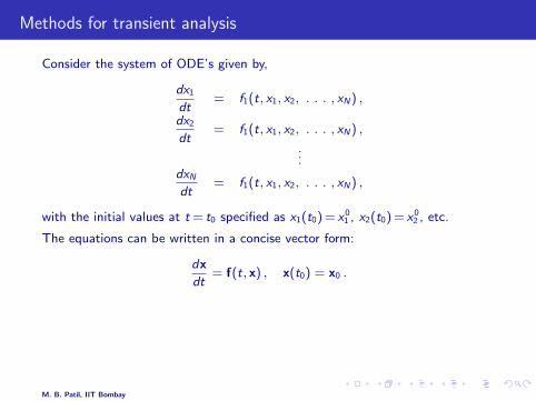
Consider the system of ODE’s given by,
dx1
dt= f1(t, x1, x2, . . . , xN ) ,
dx2
dt= f1(t, x1, x2, . . . , xN ) ,
...dxN
dt= f1(t, x1, x2, . . . , xN ) ,
with the initial values at t = t0 specified as x1(t0) = x01 , x2(t0) = x0
2 , etc.
The equations can be written in a concise vector form:
dx
dt= f(t, x) , x(t0) = x0 .
We will consider the special case of a single ODE:
dx
dt= f (t, x) , x(t0) = x0 .
M. B. Patil, IIT Bombay
Methods for transient analysis
Consider the system of ODE’s given by,
dx1
dt= f1(t, x1, x2, . . . , xN ) ,
dx2
dt= f1(t, x1, x2, . . . , xN ) ,
...dxN
dt= f1(t, x1, x2, . . . , xN ) ,
with the initial values at t = t0 specified as x1(t0) = x01 , x2(t0) = x0
2 , etc.
The equations can be written in a concise vector form:
dx
dt= f(t, x) , x(t0) = x0 .
We will consider the special case of a single ODE:
dx
dt= f (t, x) , x(t0) = x0 .
M. B. Patil, IIT Bombay
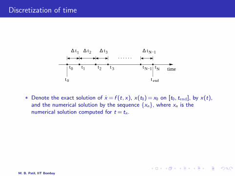
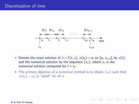
Discretization of time
∆∆∆∆ t t t t
time
2 31 N−1
t t t t t tNN−1
t t end
. . . . . .
2 30 1
0
* Denote the exact solution of x = f (t, x), x(t0) = x0 on [t0, tend], by x(t),and the numerical solution by the sequence xn, where xn is thenumerical solution computed for t = tn.
* The primary objective of a numerical method is to obtain xn such that|x(tn)− xn| is “small” for all n.
M. B. Patil, IIT Bombay

What is a “well-posed” problem?
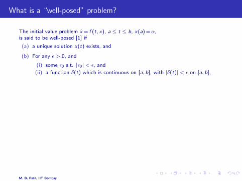
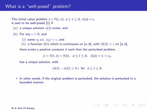
The initial value problem x = f (t, x), a ≤ t ≤ b, x(a) =α,is said to be well-posed [1] if
(a) a unique solution x(t) exists, and
(b) For any ε > 0, and
(i) some ε0 s.t. |ε0| < ε, and
(ii) a function δ(t) which is continuous on [a, b], with |δ(t)| < ε on [a, b],
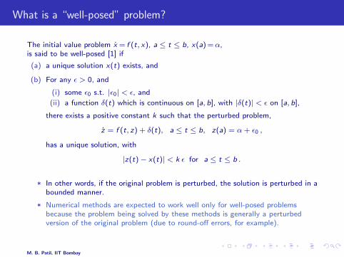
there exists a positive constant k such that the perturbed problem,
z = f (t, z) + δ(t), a ≤ t ≤ b, z(a) = α+ ε0 ,
has a unique solution, with
|z(t)− x(t)| < k ε for a ≤ t ≤ b .
* In other words, if the original problem is perturbed, the solution is perturbed in abounded manner.
* Numerical methods are expected to work well only for well-posed problemsbecause the problem being solved by these methods is generally a perturbedversion of the original problem (due to round-off errors, for example).
M. B. Patil, IIT Bombay

What is a “well-posed” problem?
The initial value problem x = f (t, x), a ≤ t ≤ b, x(a) =α,is said to be well-posed [1] if
(a) a unique solution x(t) exists, and
(b) For any ε > 0, and
(i) some ε0 s.t. |ε0| < ε, and
(ii) a function δ(t) which is continuous on [a, b], with |δ(t)| < ε on [a, b],
there exists a positive constant k such that the perturbed problem,
z = f (t, z) + δ(t), a ≤ t ≤ b, z(a) = α+ ε0 ,
has a unique solution, with
|z(t)− x(t)| < k ε for a ≤ t ≤ b .
* In other words, if the original problem is perturbed, the solution is perturbed in abounded manner.
* Numerical methods are expected to work well only for well-posed problemsbecause the problem being solved by these methods is generally a perturbedversion of the original problem (due to round-off errors, for example).
M. B. Patil, IIT Bombay

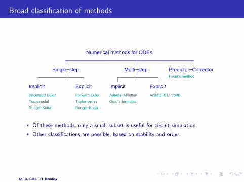
Broad classification of methods
Single−step Predictor−Corrector
ExplicitImplicit
Backward Euler
Trapezoidal
Forward Euler
Taylor series
Adams−Moulton Adams−Bashforth
Gear’s formulas
Heun’s method
Implicit
Multi−step
Runge−Kutta Runge−Kutta
Numerical methods for ODEs
Explicit
* Of these methods, only a small subset is useful for circuit simulation.
* Other classifications are possible, based on stability and order.
M. B. Patil, IIT Bombay
Local Truncation Error (LTE) and Global Error
numerical
exact
ttn+1tn tn+2
x
t
x
LTE
ǫglobal
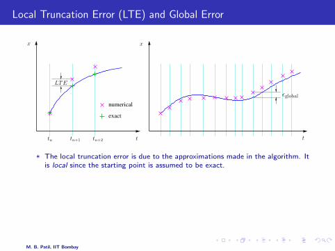
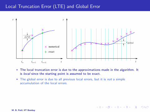
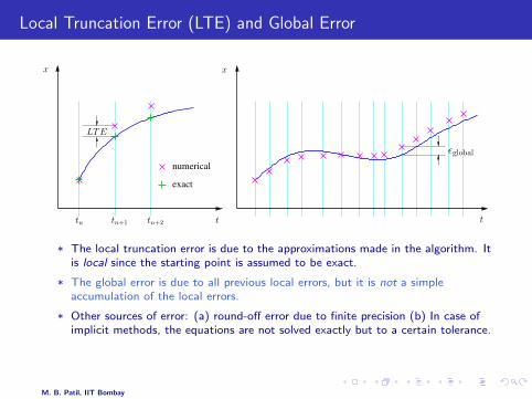
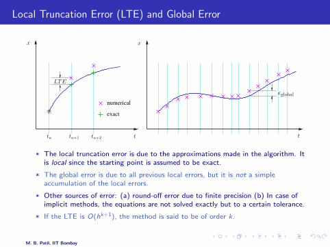
* The local truncation error is due to the approximations made in the algorithm. Itis local since the starting point is assumed to be exact.
* The global error is due to all previous local errors, but it is not a simpleaccumulation of the local errors.
* Other sources of error: (a) round-off error due to finite precision (b) In case ofimplicit methods, the equations are not solved exactly but to a certain tolerance.
* If the LTE is O(hk+1), the method is said to be of order k.
M. B. Patil, IIT Bombay
Local Truncation Error (LTE) and Global Error
numerical
exact
ttn+1tn tn+2
x
t
x
LTE
ǫglobal
* The local truncation error is due to the approximations made in the algorithm. Itis local since the starting point is assumed to be exact.
* The global error is due to all previous local errors, but it is not a simpleaccumulation of the local errors.
* Other sources of error: (a) round-off error due to finite precision (b) In case ofimplicit methods, the equations are not solved exactly but to a certain tolerance.
* If the LTE is O(hk+1), the method is said to be of order k.
M. B. Patil, IIT Bombay
Numerical methods for solving ODEs: issues of interest
* Is it one-step or multi-step?
* How is it derived?
* What is its order (accuracy)?
* What are its stability properties? (Will the method allow relatively largetime steps?)
* How is it implemented (for a single ODE and for a system of ODEs)?
* What is the computational effort per time step?
* What is the memory requirement?
M. B. Patil, IIT Bombay

Problem description
timetn−2
xn−2
fn−2
tn−1
xn−1
fn−1
tn
xn
fn
tn+1
xn+1 ?
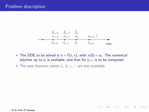
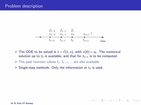
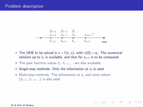
* The ODE to be solved is x = f (t, x), with x(0) = x0. The numericalsolution up to tn is available, and that for tn+1 is to be computed.
* The past function values fn, fn−1, .. are also available.
* Single-step methods: Only the information at tn is used.
* Multi-step methods: The information at tn and some others(tn−1, tn−2, ..) is also used.
M. B. Patil, IIT Bombay
Problem description
timetn−2
xn−2
fn−2
tn−1
xn−1
fn−1
tn
xn
fn
tn+1
xn+1 ?
* The ODE to be solved is x = f (t, x), with x(0) = x0. The numericalsolution up to tn is available, and that for tn+1 is to be computed.
* The past function values fn, fn−1, .. are also available.
* Single-step methods: Only the information at tn is used.
* Multi-step methods: The information at tn and some others(tn−1, tn−2, ..) is also used.
M. B. Patil, IIT Bombay

Outline
* Introduction and problem definition
* Taylor series methods
* Runge-Kutta methods
* Specific multi-step methods
* Generalized multi-step methods
* Predictor-corrector methods
* Numerical results
* Stability of numerical methods
* Regions of stability
* Stiff equations
* Adaptive step size
* Miscellaneous topics
M. B. Patil, IIT Bombay
Taylor’s theorem
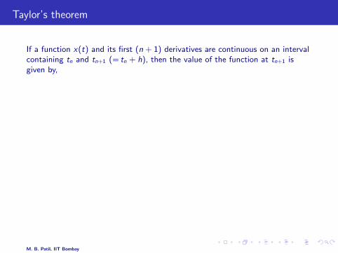
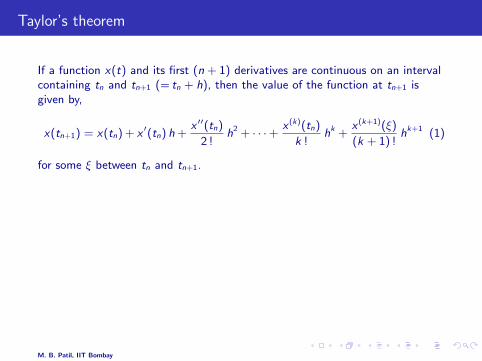
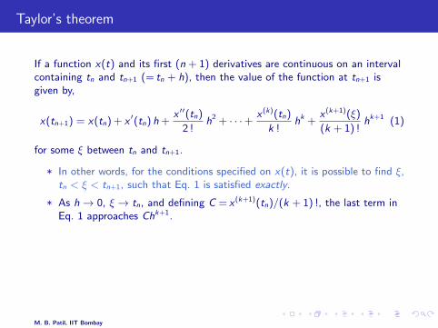
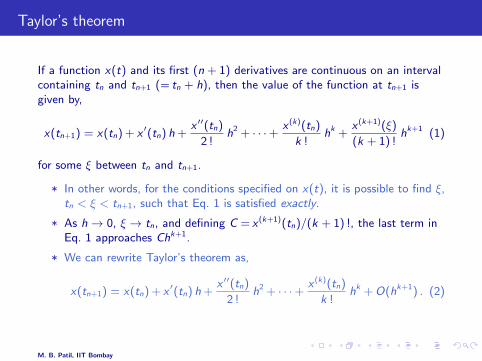
If a function x(t) and its first (n + 1) derivatives are continuous on an intervalcontaining tn and tn+1 (= tn + h), then the value of the function at tn+1 isgiven by,
x(tn+1) = x(tn) + x ′(tn) h +x ′′(tn)
2 !h2 + · · ·+ x (k)(tn)
k !hk +
x (k+1)(ξ)
(k + 1) !hk+1 (1)
for some ξ between tn and tn+1.
* In other words, for the conditions specified on x(t), it is possible to find ξ,tn < ξ < tn+1, such that Eq. 1 is satisfied exactly.
* As h→ 0, ξ → tn, and defining C = x (k+1)(tn)/(k + 1) !, the last term inEq. 1 approaches Chk+1.
* We can rewrite Taylor’s theorem as,
x(tn+1) = x(tn) + x ′(tn) h +x ′′(tn)
2 !h2 + · · ·+ x (k)(tn)
k !hk +O(hk+1) . (2)
M. B. Patil, IIT Bombay
Taylor’s theorem
If a function x(t) and its first (n + 1) derivatives are continuous on an intervalcontaining tn and tn+1 (= tn + h), then the value of the function at tn+1 isgiven by,
x(tn+1) = x(tn) + x ′(tn) h +x ′′(tn)
2 !h2 + · · ·+ x (k)(tn)
k !hk +
x (k+1)(ξ)
(k + 1) !hk+1 (1)
for some ξ between tn and tn+1.
* In other words, for the conditions specified on x(t), it is possible to find ξ,tn < ξ < tn+1, such that Eq. 1 is satisfied exactly.
* As h→ 0, ξ → tn, and defining C = x (k+1)(tn)/(k + 1) !, the last term inEq. 1 approaches Chk+1.
* We can rewrite Taylor’s theorem as,
x(tn+1) = x(tn) + x ′(tn) h +x ′′(tn)
2 !h2 + · · ·+ x (k)(tn)
k !hk +O(hk+1) . (2)
M. B. Patil, IIT Bombay

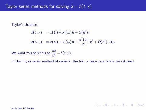
Taylor series methods for solving x = f (t, x)
Taylor’s theorem:
x(tn+1) = x(tn) + x ′(tn) h + O(h2) ,
x(tn+1) = x(tn) + x ′(tn) h +x ′′(tn)
2 !h2 + O(h3) , etc.
We want to apply this todx
dt= f (t, x) .
In the Taylor series method of order k, the first k derivative terms are retained.
xn+1 = xn + hf n ,
xn+1 = xn + hf n +h2
2(f n
t + f nf nx ) ,
where f n = f (tn, xn), f nt =
∂f
∂t(tn, xn), and f n
x =∂f
∂x(tn, xn).
M. B. Patil, IIT Bombay

Taylor series method for solving x = f (t, x)
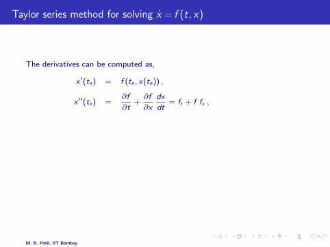
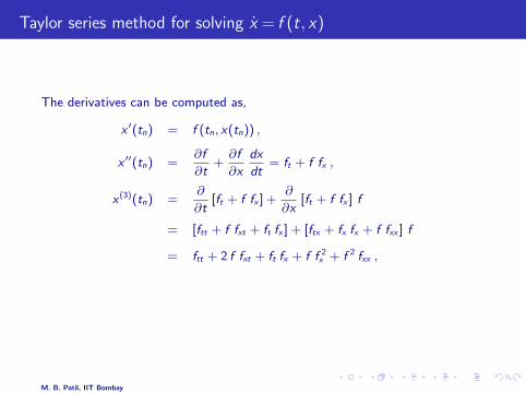
The derivatives can be computed as,
x ′(tn) = f (tn, x(tn)) ,
x ′′(tn) =∂f
∂t+∂f
∂x
dx
dt= ft + f fx ,
x (3)(tn) =∂
∂t[ft + f fx ] +
∂
∂x[ft + f fx ] f
= [ftt + f fxt + ft fx ] + [ftx + fx fx + f fxx ] f
= ftt + 2 f fxt + ft fx + f f 2x + f 2 fxx ,
Note that computation of the derivatives becomes expensive as the order
increases → Runge-Kutta methods.
M. B. Patil, IIT Bombay
Taylor series method for solving x = f (t, x)
The derivatives can be computed as,
x ′(tn) = f (tn, x(tn)) ,
x ′′(tn) =∂f
∂t+∂f
∂x
dx
dt= ft + f fx ,
x (3)(tn) =∂
∂t[ft + f fx ] +
∂
∂x[ft + f fx ] f
= [ftt + f fxt + ft fx ] + [ftx + fx fx + f fxx ] f
= ftt + 2 f fxt + ft fx + f f 2x + f 2 fxx ,
Note that computation of the derivatives becomes expensive as the order
increases → Runge-Kutta methods.
M. B. Patil, IIT Bombay

Outline
* Introduction and problem definition
* Taylor series methods
* Runge-Kutta methods
* Specific multi-step methods
* Generalized multi-step methods
* Predictor-corrector methods
* Numerical results
* Stability of numerical methods
* Regions of stability
* Stiff equations
* Adaptive step size
* Miscellaneous topics
M. B. Patil, IIT Bombay
Runge-Kutta method for solving x = f (t, x)
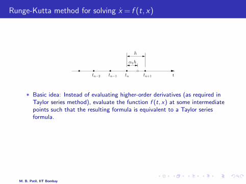
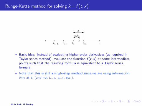
ttn−2 tn−1 tn tn+1
h
α1h
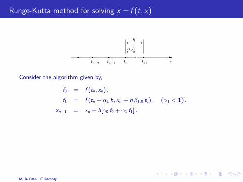
* Basic idea: Instead of evaluating higher-order derivatives (as required inTaylor series method), evaluate the function f (t, x) at some intermediatepoints such that the resulting formula is equivalent to a Taylor seriesformula.
* Note that this is still a single-step method since we are using informationonly at tn (and not tn−1, tn−2, etc.).
M. B. Patil, IIT Bombay
Runge-Kutta method for solving x = f (t, x)
ttn−2 tn−1 tn tn+1
h
α1h
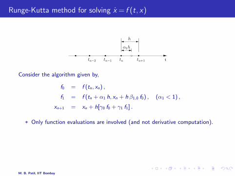
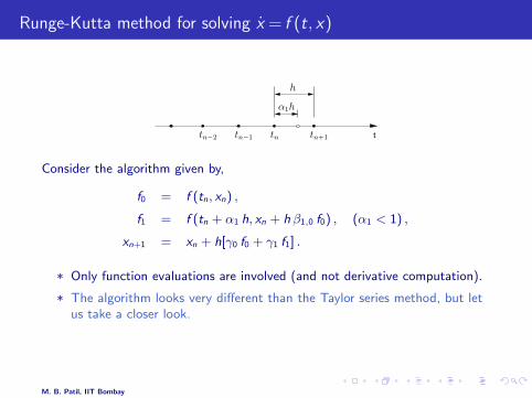
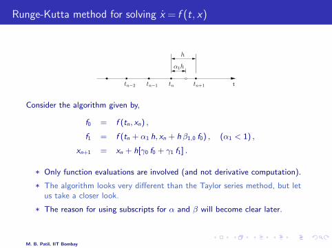
Consider the algorithm given by,
f0 = f (tn, xn) ,
f1 = f (tn + α1 h, xn + h β1,0 f0) , (α1 < 1) ,
xn+1 = xn + h[γ0 f0 + γ1 f1] .
* Only function evaluations are involved (and not derivative computation).
* The algorithm looks very different than the Taylor series method, but letus take a closer look.
* The reason for using subscripts for α and β will become clear later.
M. B. Patil, IIT Bombay
Runge-Kutta method for solving x = f (t, x)
ttn−2 tn−1 tn tn+1
h
α1h
Consider the algorithm given by,
f0 = f (tn, xn) ,
f1 = f (tn + α1 h, xn + h β1,0 f0) , (α1 < 1) ,
xn+1 = xn + h[γ0 f0 + γ1 f1] .
* Only function evaluations are involved (and not derivative computation).
* The algorithm looks very different than the Taylor series method, but letus take a closer look.
* The reason for using subscripts for α and β will become clear later.
M. B. Patil, IIT Bombay
Runge-Kutta method for solving x = f (t, x)
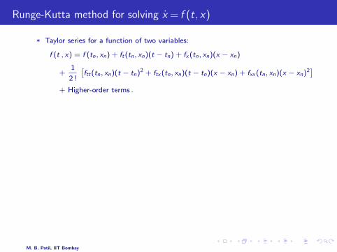
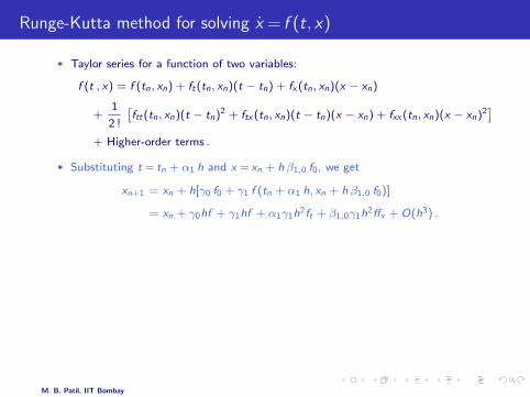
* Taylor series for a function of two variables:
f (t , x) = f (tn, xn) + ft (tn, xn)(t − tn) + fx (tn, xn)(x − xn)
+1
2 !
[ftt (tn, xn)(t − tn)2 + ftx (tn, xn)(t − tn)(x − xn) + fxx (tn, xn)(x − xn)2
]+ Higher-order terms .
* Substituting t = tn + α1 h and x = xn + h β1,0 f0, we get
xn+1 = xn + h[γ0 f0 + γ1 f (tn + α1 h, xn + h β1,0 f0)]
= xn + γ0hf + γ1hf + α1γ1h2ft + β1,0γ1h2ffx + O(h3) .
* Compare with the second-order Taylor series method,
xn+1 = xn + h f +h2
2(ft + f fx ) .
* With the conditions,γ0 + γ1 = 1 ,
α1γ1 = 1/2 ,
β1,0γ1 = 1/2 ,
the two algorithms are the same to O(h2).
M. B. Patil, IIT Bombay
Runge-Kutta method for solving x = f (t, x)
* Taylor series for a function of two variables:
f (t , x) = f (tn, xn) + ft (tn, xn)(t − tn) + fx (tn, xn)(x − xn)
+1
2 !
[ftt (tn, xn)(t − tn)2 + ftx (tn, xn)(t − tn)(x − xn) + fxx (tn, xn)(x − xn)2
]+ Higher-order terms .
* Substituting t = tn + α1 h and x = xn + h β1,0 f0, we get
xn+1 = xn + h[γ0 f0 + γ1 f (tn + α1 h, xn + h β1,0 f0)]
= xn + γ0hf + γ1hf + α1γ1h2ft + β1,0γ1h2ffx + O(h3) .
* Compare with the second-order Taylor series method,
xn+1 = xn + h f +h2
2(ft + f fx ) .
* With the conditions,γ0 + γ1 = 1 ,
α1γ1 = 1/2 ,
β1,0γ1 = 1/2 ,
the two algorithms are the same to O(h2).
M. B. Patil, IIT Bombay
Runge-Kutta method for solving x = f (t, x)
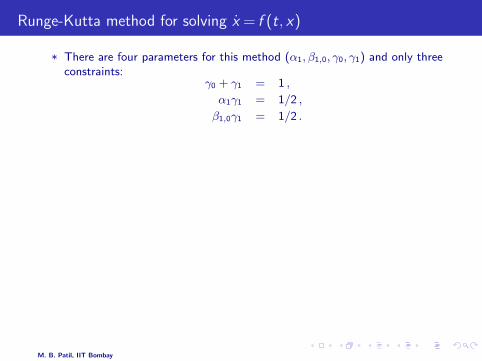
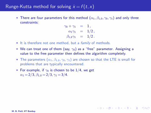
* There are four parameters for this method (α1, β1,0, γ0, γ1) and only threeconstraints:
γ0 + γ1 = 1 ,
α1γ1 = 1/2 ,
β1,0γ1 = 1/2 .
* It is therefore not one method, but a family of methods.
* We can treat one of them (say, γ0) as a “free” parameter. Assigning avalue to the free parameter then defines the algorithm completely.
* The parameters (α1, β1,0, γ0, γ1) are chosen so that the LTE is small forproblems that are typically encountered.
* For example, if γ0 is chosen to be 1/4, we getα1 = 2/3, β1,0 = 2/3, γ1 = 3/4.
* The corresponding algorithm is,
f0 = f (tn, xn) ,
f1 = f (tn + 23h, xn + 2
3hf0) ,
xn+1 = xn + h [ 14f0 + 3
4f1] .
M. B. Patil, IIT Bombay

Runge-Kutta method for solving x = f (t, x)
* There are four parameters for this method (α1, β1,0, γ0, γ1) and only threeconstraints:
γ0 + γ1 = 1 ,
α1γ1 = 1/2 ,
β1,0γ1 = 1/2 .
* It is therefore not one method, but a family of methods.
* We can treat one of them (say, γ0) as a “free” parameter. Assigning avalue to the free parameter then defines the algorithm completely.
* The parameters (α1, β1,0, γ0, γ1) are chosen so that the LTE is small forproblems that are typically encountered.
* For example, if γ0 is chosen to be 1/4, we getα1 = 2/3, β1,0 = 2/3, γ1 = 3/4.
* The corresponding algorithm is,
f0 = f (tn, xn) ,
f1 = f (tn + 23h, xn + 2
3hf0) ,
xn+1 = xn + h [ 14f0 + 3
4f1] .
M. B. Patil, IIT Bombay

Butcher array representation of RK methods [4]
f0 f1 · · · fs−1 fs
α0 β0,0 β0,1 β0,s−1 β0,s X0
α1 β1,0 β1,1 β1,s−1 β1,s X1
......
αs βs,0 βs,1 βs,s−1 βs,s Xs
γ0 γ1 · · · γs−1 γs
Interpretation: For i = 0, 1, · · · , s,
Ti = tn + αi h ,
Xi = xn + hs∑
j=0
βi,j fj ,
fi = f (Ti ,Xi ) .
Finally,
xn+1 = xn + hs∑
i=0
γi fi .
M. B. Patil, IIT Bombay
Explicit RK methods
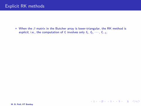
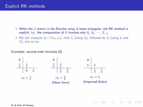
* When the β matrix in the Butcher array is lower-triangular, the RK method isexplicit, i.e., the computation of fi involves only f1, f2, · · · , fi−1.
* We can compute f0 = f (tn, xn), then f1 (using f0), followed by f2 (using f0 andf1), and so on.
Examples: second-order formulas [4]
0
12
12
0 1
α1 = 12
0
23
2314
34
α1 = 23
(Heun form)
0
1 1
12
12
α1 = 1
(Improved Euler)
M. B. Patil, IIT Bombay

Explicit RK methods
* When the β matrix in the Butcher array is lower-triangular, the RK method isexplicit, i.e., the computation of fi involves only f1, f2, · · · , fi−1.
* We can compute f0 = f (tn, xn), then f1 (using f0), followed by f2 (using f0 andf1), and so on.
Examples: second-order formulas [4]
0
12
12
0 1
α1 = 12
0
23
2314
34
α1 = 23
(Heun form)
0
1 1
12
12
α1 = 1
(Improved Euler)
M. B. Patil, IIT Bombay
Explicit RK methods
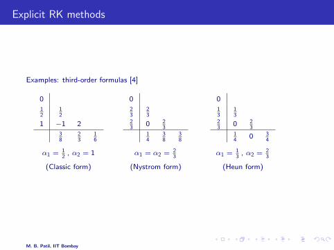
Examples: third-order formulas [4]
0
12
12
1 −1 2
38
23
16
α1 = 12
, α2 = 1
(Classic form)
0
23
23
23
0 23
14
38
38
α1 = α2 = 23
(Nystrom form)
0
13
13
23
0 23
14
0 34
α1 = 13
, α2 = 23
(Heun form)
M. B. Patil, IIT Bombay
Explicit RK methods
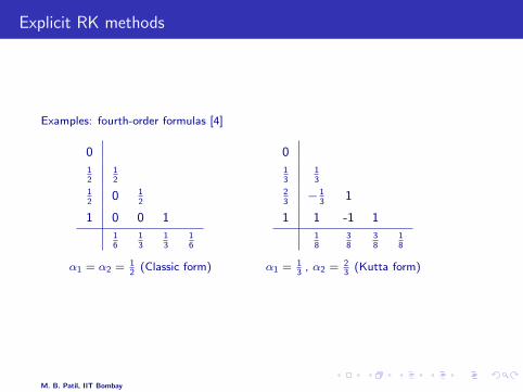
Examples: fourth-order formulas [4]
0
12
12
12
0 12
1 0 0 1
16
13
13
16
α1 = α2 = 12
(Classic form)
0
13
13
23− 1
31
1 1 -1 1
18
38
38
18
α1 = 13
, α2 = 23
(Kutta form)
M. B. Patil, IIT Bombay
Implicit RK methods
* When there are non-zero entries on the diagonal or in the upper triangle of the βmatrix of the Butcher array, the corresponding RK method is an implicitmethod.
* In this case, computation of fi may involve fi , fi+1, etc., thus ruling out a simplesuccessive computation of f0, f1, f2,· · · (which is possible for explicit RKmethods).
* Computation of fi would then require an iterative procedure, which makes itexpensive.
However, implicit methods have some advantages:
* An implicit RK formula may allow a higher order as compared to an explicit RKformula with the same number of stages.
* Implicit formulas generally have better stability properties.
M. B. Patil, IIT Bombay

Implicit RK methods [4]
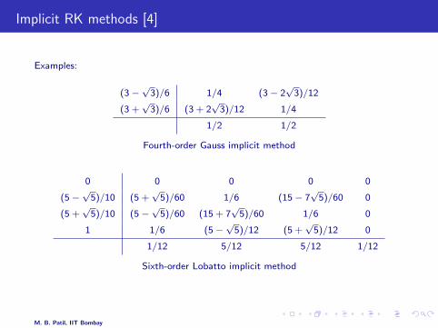
Examples:
(3−√
3)/6 1/4 (3− 2√
3)/12
(3 +√
3)/6 (3 + 2√
3)/12 1/4
1/2 1/2
Fourth-order Gauss implicit method
0 0 0 0 0
(5−√
5)/10 (5 +√
5)/60 1/6 (15− 7√
5)/60 0
(5 +√
5)/10 (5−√
5)/60 (15 + 7√
5)/60 1/6 0
1 1/6 (5−√
5)/12 (5 +√
5)/12 0
1/12 5/12 5/12 1/12
Sixth-order Lobatto implicit method
M. B. Patil, IIT Bombay
Implicit RK methods [4]
Examples:
(3−√
3)/6 1/4 (3− 2√
3)/12
(3 +√
3)/6 (3 + 2√
3)/12 1/4
1/2 1/2
Fourth-order Gauss implicit method
0 0 0 0 0
(5−√
5)/10 (5 +√
5)/60 1/6 (15− 7√
5)/60 0
(5 +√
5)/10 (5−√
5)/60 (15 + 7√
5)/60 1/6 0
1 1/6 (5−√
5)/12 (5 +√
5)/12 0
1/12 5/12 5/12 1/12
Sixth-order Lobatto implicit method
M. B. Patil, IIT Bombay

RK method: system of equations
The RK methods (both explicit and implicit) can be used to solve a system of ODEs,
dx
dt= f(t, x) , x(t0) = x0 .
The computation involves the following:
For i = 0, 1, · · · , s,
Ti = tn + αi h ,
Xi = xn + hs∑
j=0
βi,j fj ,
fj = f (Ti ,Xi) ,
and finally,
xn+1 = xn + hs∑
i=0
γi fi .
M. B. Patil, IIT Bombay

Outline
* Introduction and problem definition
* Taylor series methods
* Runge-Kutta methods
* Specific multi-step methods
* Generalized multi-step methods
* Predictor-corrector methods
* Numerical results
* Stability of numerical methods
* Regions of stability
* Stiff equations
* Adaptive step size
* Miscellaneous topics
M. B. Patil, IIT Bombay
Multi-step methods for solving x = f (t, x)
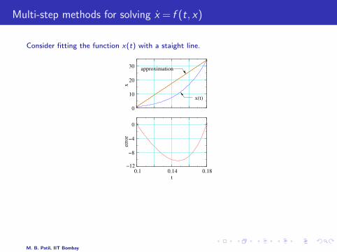
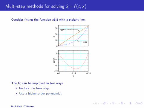
Consider fitting the function x(t) with a staight line.
−8
−4
0
0.1 0.14 0.18t
erro
r
−12
0
10
20
30
x
x(t)
approximation
The fit can be improved in two ways:
* Reduce the time step.
* Use a higher-order polynomial.
M. B. Patil, IIT Bombay

Multi-step methods for solving x = f (t, x)
Consider fitting the function x(t) with a staight line.
−8
−4
0
0.1 0.14 0.18t
erro
r
−12
0
10
20
30
x
x(t)
approximation
The fit can be improved in two ways:
* Reduce the time step.
* Use a higher-order polynomial.
M. B. Patil, IIT Bombay

Multi-step methods for solving x = f (t, x)
Consider fitting the function x(t) with a staight line.
−8
−4
0
0.1 0.14 0.18t
erro
r
−12
0
10
20
30
x
x(t)
approximation
The fit can be improved in two ways:
* Reduce the time step.
* Use a higher-order polynomial.
M. B. Patil, IIT Bombay
Multi-step methods for solving x = f (t, x)
Consider fitting the function x(t) with a staight line.
−8
−4
0
0.1 0.14 0.18t
erro
r
−12
0
10
20
30
x
x(t)
approximation
The fit can be improved in two ways:
* Reduce the time step.
* Use a higher-order polynomial.
M. B. Patil, IIT Bombay

Multi-step methods for solving x = f (t, x)
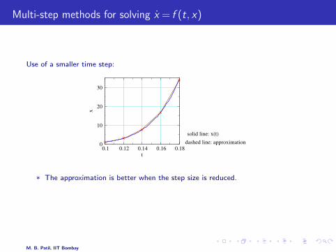
Use of a smaller time step:
0
10
20
30
0.1 0.12 0.14 0.16 0.18
x
t
dashed line: approximation
solid line: x(t)
* The approximation is better when the step size is reduced.
* A larger number of time steps ⇒ slower simulation
M. B. Patil, IIT Bombay
Multi-step methods for solving x = f (t, x)
Use of a smaller time step:
0
10
20
30
0.1 0.12 0.14 0.16 0.18
x
t
dashed line: approximation
solid line: x(t)
* The approximation is better when the step size is reduced.
* A larger number of time steps ⇒ slower simulation
M. B. Patil, IIT Bombay

Multi-step methods for solving x = f (t, x)
Use of a smaller time step:
0
10
20
30
0.1 0.12 0.14 0.16 0.18
x
t
dashed line: approximation
solid line: x(t)
* The approximation is better when the step size is reduced.
* A larger number of time steps ⇒ slower simulation
M. B. Patil, IIT Bombay

Multi-step methods for solving x = f (t, x)
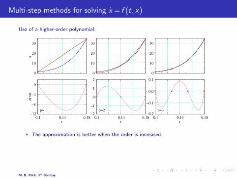
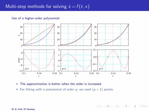
Use of a higher-order polynomial:
p=1 p=2 p=3 −1
0
1
2
−0.1
0.0
0.1
0.1 0.14 0.18
t
0.1 0.14 0.18
t
−8
−4
0
0.1 0.14 0.18
t
erro
r
−12 −2 −0.2
0
10
20
30
x
0
10
20
30
0
10
20
30
* The approximation is better when the order is increased.
* For fitting with a polynomial of order p, we need (p + 1) points.
* The Adams-Bashforth and Adams-Moulton methods are based on approximatingx(t) with a polynomial.
M. B. Patil, IIT Bombay
Multi-step methods for solving x = f (t, x)
Use of a higher-order polynomial:
p=1 p=2 p=3 −1
0
1
2
−0.1
0.0
0.1
0.1 0.14 0.18
t
0.1 0.14 0.18
t
−8
−4
0
0.1 0.14 0.18
t
erro
r
−12 −2 −0.2
0
10
20
30
x
0
10
20
30
0
10
20
30
* The approximation is better when the order is increased.
* For fitting with a polynomial of order p, we need (p + 1) points.
* The Adams-Bashforth and Adams-Moulton methods are based on approximatingx(t) with a polynomial.
M. B. Patil, IIT Bombay
Adams-Bashforth methods for x = f (t, x)
t tt t t tn−2n−3n−4 n−1 n n+1 t
f
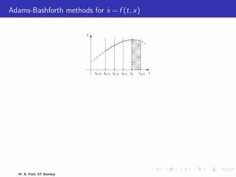
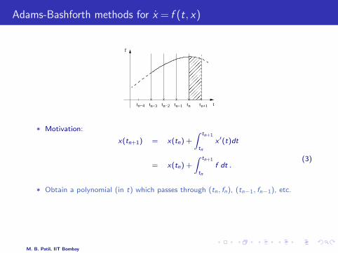
* Motivation:
x(tn+1) = x(tn) +
∫ tn+1
tn
x ′(t)dt
= x(tn) +
∫ tn+1
tn
f dt .(3)
* Obtain a polynomial (in t) which passes through (tn, fn), (tn−1, fn−1), etc.
* Compute
∫ tn+1
tn
f dt in Eq. 3 using the approximation for f ⇒ Adams-Bashforth
formula.
M. B. Patil, IIT Bombay

Adams-Bashforth methods for x = f (t, x)
t tt t t tn−2n−3n−4 n−1 n n+1 t
f
* Motivation:
x(tn+1) = x(tn) +
∫ tn+1
tn
x ′(t)dt
= x(tn) +
∫ tn+1
tn
f dt .(3)
* Obtain a polynomial (in t) which passes through (tn, fn), (tn−1, fn−1), etc.
* Compute
∫ tn+1
tn
f dt in Eq. 3 using the approximation for f ⇒ Adams-Bashforth
formula.
M. B. Patil, IIT Bombay

Adams-Bashforth methods for x = f (t, x)
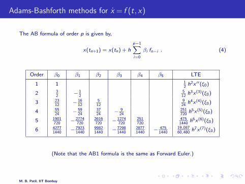
The AB formula of order p is given by,
x(tn+1) = x(tn) + h
p−1∑i=0
βi fn−i . (4)
Order β0 β1 β2 β3 β4 β5 LTE
1 1 12
h2x ′′(ξ0)
2 32
− 12
512
h3x(3)(ξ0)
3 2312
− 1612
512
924
h4x(4)(ξ0)
4 5524
− 5924
3724
− 924
251720
h5x(5)(ξ0)
5 1901720
− 2774720
2616720
− 1274720
251720
4751440
h6x(6)(ξ0)
6 42771440
− 79231440
99821440
− 72981440
28771440
− 4751440
19,08760,480
h7x(7)(ξ0)
(Note that the AB1 formula is the same as Forward Euler.)
M. B. Patil, IIT Bombay
Adams-Bashforth methods for x = f (t, x)
The AB formula of order p is given by,
x(tn+1) = x(tn) + h
p−1∑i=0
βi fn−i . (4)
Order β0 β1 β2 β3 β4 β5 LTE
1 1 12
h2x ′′(ξ0)
2 32
− 12
512
h3x(3)(ξ0)
3 2312
− 1612
512
924
h4x(4)(ξ0)
4 5524
− 5924
3724
− 924
251720
h5x(5)(ξ0)
5 1901720
− 2774720
2616720
− 1274720
251720
4751440
h6x(6)(ξ0)
6 42771440
− 79231440
99821440
− 72981440
28771440
− 4751440
19,08760,480
h7x(7)(ξ0)
(Note that the AB1 formula is the same as Forward Euler.)
M. B. Patil, IIT Bombay
Adams-Moulton methods for x = f (t, x)
t tt t t tn−2n−3n−4 n−1 n n+1
f
t
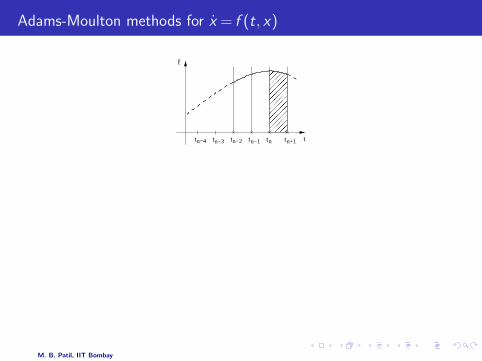
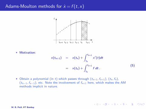
* Motivation:
x(tn+1) = x(tn) +
∫ tn+1
tn
x ′(t)dt
= x(tn) +
∫ tn+1
tn
f dt .(5)
* Obtain a polynomial (in t) which passes through (tn+1, fn+1), (tn, fn),(tn−1, fn−1), etc. Note the involvement of fn+1 here, which makes the AMmethods implicit in nature.
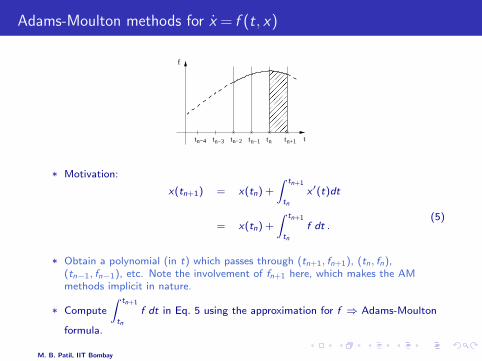
* Compute
∫ tn+1
tn
f dt in Eq. 5 using the approximation for f ⇒ Adams-Moulton
formula.
M. B. Patil, IIT Bombay

Adams-Moulton methods for x = f (t, x)
t tt t t tn−2n−3n−4 n−1 n n+1
f
t
* Motivation:
x(tn+1) = x(tn) +
∫ tn+1
tn
x ′(t)dt
= x(tn) +
∫ tn+1
tn
f dt .(5)
* Obtain a polynomial (in t) which passes through (tn+1, fn+1), (tn, fn),(tn−1, fn−1), etc. Note the involvement of fn+1 here, which makes the AMmethods implicit in nature.
* Compute
∫ tn+1
tn
f dt in Eq. 5 using the approximation for f ⇒ Adams-Moulton
formula.
M. B. Patil, IIT Bombay

Adams-Moulton methods for x = f (t, x)
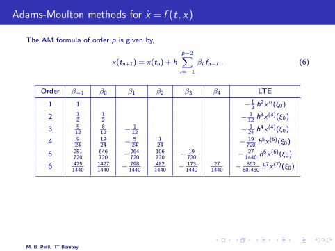
The AM formula of order p is given by,
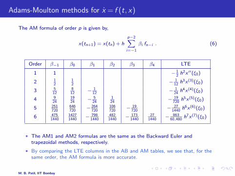
x(tn+1) = x(tn) + h
p−2∑i=−1
βi fn−i . (6)
Order β−1 β0 β1 β2 β3 β4 LTE
1 1 − 12
h2x ′′(ξ0)
2 12
12
− 112
h3x(3)(ξ0)
3 512
812
− 112
− 124
h4x(4)(ξ0)
4 924
1924
− 524
124
− 19720
h5x(5)(ξ0)
5 251720
646720
− 264720
106720
− 19720
− 271440
h6x(6)(ξ0)
6 4751440
14271440
− 7981440
4821440
− 1731440
271440
− 86360,480
h7x(7)(ξ0)
* The AM1 and AM2 formulas are the same as the Backward Euler andtrapezoidal methods, respectively.
* By comparing the LTE columns in the AB and AM tables, we see that, for thesame order, the AM formula is more accurate.
M. B. Patil, IIT Bombay
Adams-Moulton methods for x = f (t, x)
The AM formula of order p is given by,
x(tn+1) = x(tn) + h
p−2∑i=−1
βi fn−i . (6)
Order β−1 β0 β1 β2 β3 β4 LTE
1 1 − 12
h2x ′′(ξ0)
2 12
12
− 112
h3x(3)(ξ0)
3 512
812
− 112
− 124
h4x(4)(ξ0)
4 924
1924
− 524
124
− 19720
h5x(5)(ξ0)
5 251720
646720
− 264720
106720
− 19720
− 271440
h6x(6)(ξ0)
6 4751440
14271440
− 7981440
4821440
− 1731440
271440
− 86360,480
h7x(7)(ξ0)
* The AM1 and AM2 formulas are the same as the Backward Euler andtrapezoidal methods, respectively.
* By comparing the LTE columns in the AB and AM tables, we see that, for thesame order, the AM formula is more accurate.
M. B. Patil, IIT Bombay

Backward Differentiation Formulas (BDF): Gear’s formulas
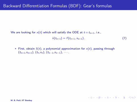
We are looking for x(t) which will satisfy the ODE at t = tn+1, i.e.,
x(tn+1) = f (tn+1, xn+1) . (7)
* First, obtain x(t), a polynomial approximation for x(t), passing through(tn+1,xn+1), (tn,xn), (tn−1,xn−1), · · · .
* Differentiate to get an expression for ˜x(t).
* Replace the LHS of Eq. 7 with ˜x(t) at t = tn+1. ⇒ BDF formula
* BDFs are implicit in nature since f (tn+1, xn+1) appears in the formula.
M. B. Patil, IIT Bombay
Backward Differentiation Formulas (BDF): Gear’s formulas
We are looking for x(t) which will satisfy the ODE at t = tn+1, i.e.,
x(tn+1) = f (tn+1, xn+1) . (7)
* First, obtain x(t), a polynomial approximation for x(t), passing through(tn+1,xn+1), (tn,xn), (tn−1,xn−1), · · · .
* Differentiate to get an expression for ˜x(t).
* Replace the LHS of Eq. 7 with ˜x(t) at t = tn+1. ⇒ BDF formula
* BDFs are implicit in nature since f (tn+1, xn+1) appears in the formula.
M. B. Patil, IIT Bombay
BDFs for x = f (t, x)
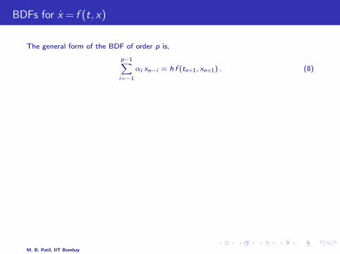
The general form of the BDF of order p is,
p−1∑i=−1
αi xn−i = h f (tn+1, xn+1) . (8)
Order α−1 α0 α1 α2 α3 α4 α5 LTE
1 1 −1 − 12
h2x ′′(ξ)
2 32
−2 12
− 29
h3x ′′′(ξ)
3 116
−3 − 32
− 13
− 322
h4x(4)(ξ)
4 2512
−4 3 − 43
14
− 12125
h5x(5)(ξ)
5 13760
−5 5 − 103
54
− 15
− 10137
h6x(6)(ξ)
6 14760
−6 152
− 203
154
− 65
16
− 601029
h7x(7)(ξ)
(Note that the BDF1 formula is the same as the Backward Euler method.)
M. B. Patil, IIT Bombay

BDFs for x = f (t, x)
The general form of the BDF of order p is,
p−1∑i=−1
αi xn−i = h f (tn+1, xn+1) . (8)
Order α−1 α0 α1 α2 α3 α4 α5 LTE
1 1 −1 − 12
h2x ′′(ξ)
2 32
−2 12
− 29
h3x ′′′(ξ)
3 116
−3 − 32
− 13
− 322
h4x(4)(ξ)
4 2512
−4 3 − 43
14
− 12125
h5x(5)(ξ)
5 13760
−5 5 − 103
54
− 15
− 10137
h6x(6)(ξ)
6 14760
−6 152
− 203
154
− 65
16
− 601029
h7x(7)(ξ)
(Note that the BDF1 formula is the same as the Backward Euler method.)
M. B. Patil, IIT Bombay

Outline
* Introduction and problem definition
* Taylor series methods
* Runge-Kutta methods
* Specific multi-step methods
* Generalized multi-step methods
* Predictor-corrector methods
* Numerical results
* Stability of numerical methods
* Regions of stability
* Stiff equations
* Adaptive step size
* Miscellaneous topics
M. B. Patil, IIT Bombay

Generalized linear multi-step methods
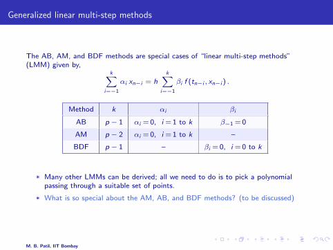
The AB, AM, and BDF methods are special cases of “linear multi-step methods”(LMM) given by,
k∑i=−1
αi xn−i = hk∑
i=−1
βi f (tn−i , xn−i ) .
Method k αi βi
AB p − 1 αi = 0, i = 1 to k β−1 = 0
AM p − 2 αi = 0, i = 1 to k –
BDF p − 1 – βi = 0, i = 0 to k
* Many other LMMs can be derived; all we need to do is to pick a polynomialpassing through a suitable set of points.
* What is so special about the AM, AB, and BDF methods? (to be discussed)
M. B. Patil, IIT Bombay

Generalized linear multi-step methods
The AB, AM, and BDF methods are special cases of “linear multi-step methods”(LMM) given by,
k∑i=−1
αi xn−i = hk∑
i=−1
βi f (tn−i , xn−i ) .
Method k αi βi
AB p − 1 αi = 0, i = 1 to k β−1 = 0
AM p − 2 αi = 0, i = 1 to k –
BDF p − 1 – βi = 0, i = 0 to k
* Many other LMMs can be derived; all we need to do is to pick a polynomialpassing through a suitable set of points.
* What is so special about the AM, AB, and BDF methods? (to be discussed)
M. B. Patil, IIT Bombay

Exactness constraints for LMMs [6] for solving x = f (t, x)
tn+1tntn−1tn−2
h0t−h−2h
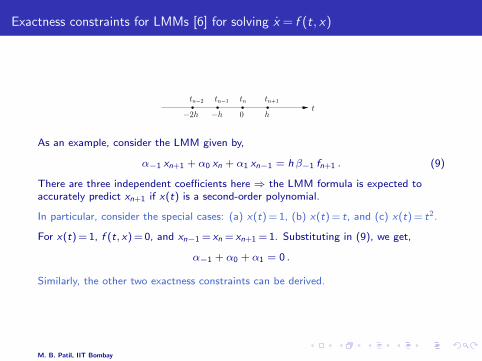
As an example, consider the LMM given by,
α−1 xn+1 + α0 xn + α1 xn−1 = h β−1 fn+1 . (9)
There are three independent coefficients here ⇒ the LMM formula is expected toaccurately predict xn+1 if x(t) is a second-order polynomial.
In particular, consider the special cases: (a) x(t) = 1, (b) x(t) = t, and (c) x(t) = t2.
For x(t) = 1, f (t, x) = 0, and xn−1 = xn = xn+1 = 1. Substituting in (9), we get,
α−1 + α0 + α1 = 0 .
Similarly, the other two exactness constraints can be derived.
M. B. Patil, IIT Bombay

Exactness constraints for LMMs [6] for solving x = f (t, x)
tn+1tntn−1tn−2
h0t−h−2h
As an example, consider the LMM given by,
α−1 xn+1 + α0 xn + α1 xn−1 = h β−1 fn+1 . (9)
There are three independent coefficients here ⇒ the LMM formula is expected toaccurately predict xn+1 if x(t) is a second-order polynomial.
In particular, consider the special cases: (a) x(t) = 1, (b) x(t) = t, and (c) x(t) = t2.
For x(t) = 1, f (t, x) = 0, and xn−1 = xn = xn+1 = 1. Substituting in (9), we get,
α−1 + α0 + α1 = 0 .
Similarly, the other two exactness constraints can be derived.
M. B. Patil, IIT Bombay

Exactness constraints for LMMs for solving x = f (t, x)
x f xn+1 Constraint
1 0 1 α−1 + α0 + α1 = 0
t 1 h α−1 − α1 = β−1
t2 2 t h2 α−1 + α1 = 2β−1
* With β−1 = 1, we get α−1 = 3/2, α0 =−2, and α1 = 1/2.
* The LMM formula is therefore,
3
2xn+1 − 2 xn +
1
2xn−1 = h fn+1 .
* This is the same as the BDF2 formula.
M. B. Patil, IIT Bombay

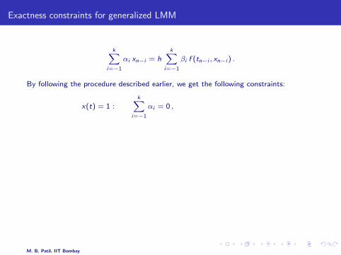
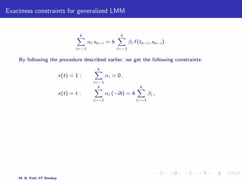
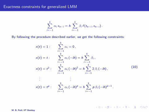
Exactness constraints for generalized LMM
k∑i=−1
αi xn−i = hk∑
i=−1
βi f (tn−i , xn−i ) .
By following the procedure described earlier, we get the following constraints:
x(t) = 1 :k∑
i=−1
αi = 0 ,
x(t) = t :k∑
i=−1
αi (−ih) = hk∑
i=−1
βi ,
x(t) = t2 :k∑
i=−1
αi (−ih)2 = hk∑
i=−1
2βi (−ih) ,
......
x(t) = tp :k∑
i=−1
αi (−ih)p = hk∑
i=−1
p βi (−ih)p−1 .
(10)
M. B. Patil, IIT Bombay

Outline
* Introduction and problem definition
* Taylor series methods
* Runge-Kutta methods
* Specific multi-step methods
* Generalized multi-step methods
* Predictor-corrector methods
* Numerical results
* Stability of numerical methods
* Regions of stability
* Stiff equations
* Adaptive step size
* Miscellaneous topics
M. B. Patil, IIT Bombay

Predictor-corrector methods
* For the same order, AM methods are more accurate than AB methods.
* AB methods are explicit whereas AM methods are implicit.⇒ For the same order, the AB method is faster.
* Can we combine the best of the AB and AM methods?⇒ Predictor-Corrector (PC) methods
* In the PC method, in going from tn to tn+1,
- “Predict” xn+1 using an explicit method (such as AB).- “Correct” xn+1 using an implicit method (such as AM). However, in this
step, use the implicit formula as an “evaluation” formula, i.e., treat xn+1 inthe RHS as a known value (given by the predicted xn+1).
- Repeat to the desired tolerance.
M. B. Patil, IIT Bombay
Predictor-corrector methods
* For the same order, AM methods are more accurate than AB methods.
* AB methods are explicit whereas AM methods are implicit.
⇒ For the same order, the AB method is faster.
* Can we combine the best of the AB and AM methods?⇒ Predictor-Corrector (PC) methods
* In the PC method, in going from tn to tn+1,
- “Predict” xn+1 using an explicit method (such as AB).- “Correct” xn+1 using an implicit method (such as AM). However, in this
step, use the implicit formula as an “evaluation” formula, i.e., treat xn+1 inthe RHS as a known value (given by the predicted xn+1).
- Repeat to the desired tolerance.
M. B. Patil, IIT Bombay
Predictor-corrector methods
* For the same order, AM methods are more accurate than AB methods.
* AB methods are explicit whereas AM methods are implicit.⇒ For the same order, the AB method is faster.
* Can we combine the best of the AB and AM methods?⇒ Predictor-Corrector (PC) methods
* In the PC method, in going from tn to tn+1,
- “Predict” xn+1 using an explicit method (such as AB).- “Correct” xn+1 using an implicit method (such as AM). However, in this
step, use the implicit formula as an “evaluation” formula, i.e., treat xn+1 inthe RHS as a known value (given by the predicted xn+1).
- Repeat to the desired tolerance.
M. B. Patil, IIT Bombay

Predictor-corrector methods
* For the same order, AM methods are more accurate than AB methods.
* AB methods are explicit whereas AM methods are implicit.⇒ For the same order, the AB method is faster.
* Can we combine the best of the AB and AM methods?
⇒ Predictor-Corrector (PC) methods
* In the PC method, in going from tn to tn+1,
- “Predict” xn+1 using an explicit method (such as AB).- “Correct” xn+1 using an implicit method (such as AM). However, in this
step, use the implicit formula as an “evaluation” formula, i.e., treat xn+1 inthe RHS as a known value (given by the predicted xn+1).
- Repeat to the desired tolerance.
M. B. Patil, IIT Bombay

Predictor-corrector methods
* For the same order, AM methods are more accurate than AB methods.
* AB methods are explicit whereas AM methods are implicit.⇒ For the same order, the AB method is faster.
* Can we combine the best of the AB and AM methods?⇒ Predictor-Corrector (PC) methods
* In the PC method, in going from tn to tn+1,
- “Predict” xn+1 using an explicit method (such as AB).- “Correct” xn+1 using an implicit method (such as AM). However, in this
step, use the implicit formula as an “evaluation” formula, i.e., treat xn+1 inthe RHS as a known value (given by the predicted xn+1).
- Repeat to the desired tolerance.
M. B. Patil, IIT Bombay

Predictor-corrector methods
* For the same order, AM methods are more accurate than AB methods.
* AB methods are explicit whereas AM methods are implicit.⇒ For the same order, the AB method is faster.
* Can we combine the best of the AB and AM methods?⇒ Predictor-Corrector (PC) methods
* In the PC method, in going from tn to tn+1,
- “Predict” xn+1 using an explicit method (such as AB).
- “Correct” xn+1 using an implicit method (such as AM). However, in thisstep, use the implicit formula as an “evaluation” formula, i.e., treat xn+1 inthe RHS as a known value (given by the predicted xn+1).
- Repeat to the desired tolerance.
M. B. Patil, IIT Bombay

Predictor-corrector methods
* For the same order, AM methods are more accurate than AB methods.
* AB methods are explicit whereas AM methods are implicit.⇒ For the same order, the AB method is faster.
* Can we combine the best of the AB and AM methods?⇒ Predictor-Corrector (PC) methods
* In the PC method, in going from tn to tn+1,
- “Predict” xn+1 using an explicit method (such as AB).- “Correct” xn+1 using an implicit method (such as AM). However, in this
step, use the implicit formula as an “evaluation” formula, i.e., treat xn+1 inthe RHS as a known value (given by the predicted xn+1).
- Repeat to the desired tolerance.
M. B. Patil, IIT Bombay
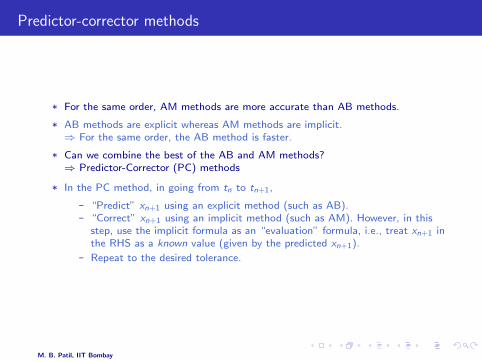
Predictor-corrector methods
* For the same order, AM methods are more accurate than AB methods.
* AB methods are explicit whereas AM methods are implicit.⇒ For the same order, the AB method is faster.
* Can we combine the best of the AB and AM methods?⇒ Predictor-Corrector (PC) methods
* In the PC method, in going from tn to tn+1,
- “Predict” xn+1 using an explicit method (such as AB).- “Correct” xn+1 using an implicit method (such as AM). However, in this
step, use the implicit formula as an “evaluation” formula, i.e., treat xn+1 inthe RHS as a known value (given by the predicted xn+1).
- Repeat to the desired tolerance.
M. B. Patil, IIT Bombay

Predictor-corrector method for solving x = f (t, x)
Example: Use AB1 as predictor and AM2 as corrector.
Prediction (P) x(0)n+1 = xn + h fn (AB1)
Evaluation (E) f(0)
n+1 = f (tn+1, x(0)n+1)
Correction (C) x(1)n+1 = xn +
h
2(fn + f
(0)n+1) (AM2)
Evaluation (E) f(1)
n+1 = f (tn+1, x(1)n+1)
* We can repeat this process, e.g., PECECE, or PE(CE)k .
* If the process is taken to covergence, we could obtain the same result as usingthe implicit (corrector) formula alone, i.e., solving the implicit equation of thecorrector exactly.
* Generally, one or two CE steps give a substantially better accuracy (over thepredicted xn+1).
M. B. Patil, IIT Bombay
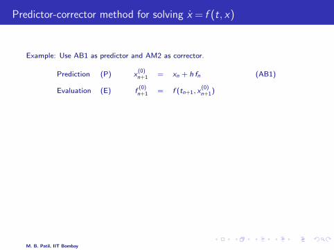
Predictor-corrector method for solving x = f (t, x)
Example: Use AB1 as predictor and AM2 as corrector.
Prediction (P) x(0)n+1 = xn + h fn (AB1)
Evaluation (E) f(0)
n+1 = f (tn+1, x(0)n+1)
Correction (C) x(1)n+1 = xn +
h
2(fn + f
(0)n+1) (AM2)
Evaluation (E) f(1)
n+1 = f (tn+1, x(1)n+1)
* We can repeat this process, e.g., PECECE, or PE(CE)k .
* If the process is taken to covergence, we could obtain the same result as usingthe implicit (corrector) formula alone, i.e., solving the implicit equation of thecorrector exactly.
* Generally, one or two CE steps give a substantially better accuracy (over thepredicted xn+1).
M. B. Patil, IIT Bombay
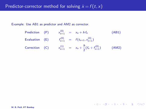
Predictor-corrector method for solving x = f (t, x)
Example: Use AB1 as predictor and AM2 as corrector.
Prediction (P) x(0)n+1 = xn + h fn (AB1)
Evaluation (E) f(0)
n+1 = f (tn+1, x(0)n+1)
Correction (C) x(1)n+1 = xn +
h
2(fn + f
(0)n+1) (AM2)
Evaluation (E) f(1)
n+1 = f (tn+1, x(1)n+1)
* We can repeat this process, e.g., PECECE, or PE(CE)k .
* If the process is taken to covergence, we could obtain the same result as usingthe implicit (corrector) formula alone, i.e., solving the implicit equation of thecorrector exactly.
* Generally, one or two CE steps give a substantially better accuracy (over thepredicted xn+1).
M. B. Patil, IIT Bombay
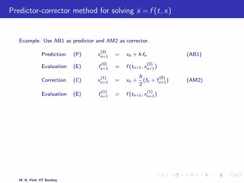
Predictor-corrector method for solving x = f (t, x)
Example: Use AB1 as predictor and AM2 as corrector.
Prediction (P) x(0)n+1 = xn + h fn (AB1)
Evaluation (E) f(0)
n+1 = f (tn+1, x(0)n+1)
Correction (C) x(1)n+1 = xn +
h
2(fn + f
(0)n+1) (AM2)
Evaluation (E) f(1)
n+1 = f (tn+1, x(1)n+1)
* We can repeat this process, e.g., PECECE, or PE(CE)k .
* If the process is taken to covergence, we could obtain the same result as usingthe implicit (corrector) formula alone, i.e., solving the implicit equation of thecorrector exactly.
* Generally, one or two CE steps give a substantially better accuracy (over thepredicted xn+1).
M. B. Patil, IIT Bombay
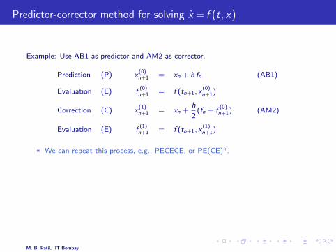
Predictor-corrector method for solving x = f (t, x)
Example: Use AB1 as predictor and AM2 as corrector.
Prediction (P) x(0)n+1 = xn + h fn (AB1)
Evaluation (E) f(0)
n+1 = f (tn+1, x(0)n+1)
Correction (C) x(1)n+1 = xn +
h
2(fn + f
(0)n+1) (AM2)
Evaluation (E) f(1)
n+1 = f (tn+1, x(1)n+1)
* We can repeat this process, e.g., PECECE, or PE(CE)k .
* If the process is taken to covergence, we could obtain the same result as usingthe implicit (corrector) formula alone, i.e., solving the implicit equation of thecorrector exactly.
* Generally, one or two CE steps give a substantially better accuracy (over thepredicted xn+1).
M. B. Patil, IIT Bombay

Predictor-corrector method for solving x = f (t, x)
Example: Use AB1 as predictor and AM2 as corrector for the ODE,
x = 2 x − x2, with x(0) = 1 (analytic solution: x(t) = 2/(1 + exp(−2t)))
step size (h) 0.05 0.1 0.2
predicted x(h) 1.05 1.1 1.2
corrected x(h) (1) 1.04993750 1.09950000 1.19600000
(2) 1.04993766 1.09950499 1.19615840
(3) 1.04993766 1.09950494 1.19615219
(4) 1.04993766 1.09950494 1.19615243
(5) 1.04993766 1.09950494 1.19615242
x(h) (TRZ) 1.04993766 1.09950494 1.19615242
x(h) (exact) 1.04995837 1.09966799 1.19737532
LTE 2.0719×10⁻⁵ 1.6306×10⁻⁴ 1.2229×10⁻³
M. B. Patil, IIT Bombay
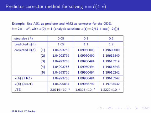
Predictor-corrector method for solving x = f (t, x)
Example: Use AB1 as predictor and AM2 as corrector for the ODE,
x = 2 x − x2, with x(0) = 1 (analytic solution: x(t) = 2/(1 + exp(−2t)))
step size (h) 0.05 0.1 0.2
predicted x(h) 1.05 1.1 1.2
corrected x(h) (1) 1.04993750 1.09950000 1.19600000
(2) 1.04993766 1.09950499 1.19615840
(3) 1.04993766 1.09950494 1.19615219
(4) 1.04993766 1.09950494 1.19615243
(5) 1.04993766 1.09950494 1.19615242
x(h) (TRZ) 1.04993766 1.09950494 1.19615242
x(h) (exact) 1.04995837 1.09966799 1.19737532
LTE 2.0719×10⁻⁵ 1.6306×10⁻⁴ 1.2229×10⁻³
M. B. Patil, IIT Bombay

Outline
* Introduction and problem definition
* Taylor series methods
* Runge-Kutta methods
* Specific multi-step methods
* Generalized multi-step methods
* Predictor-corrector methods
* Numerical results
* Stability of numerical methods
* Regions of stability
* Stiff equations
* Adaptive step size
* Miscellaneous topics
M. B. Patil, IIT Bombay

Numerical examples: local/global error versus h
global
localglobal
local
10 10 10 1010 10 10 10 10
10
10
10
10
−6
−2
(c) Trapezoidal (d) Runge−Kutta (4)
10
10
10
10
−6
−2
−10
−14
−4 −3 −2 −1 0 −3 −2 −1 0
−14
−10
global
local
global
local
10
10
10
10
10
−8
−6
−4
−2
0
10
10
10
10
10
−8
−6
−4
−2
0
10 10 10 10 10 10 10 10 10 10
(a) Forward Euler (b) Backward Euler
−4 −3 −2 −1 0 −4 −3 −2 −1 0
step size (h) step size (h)
Err
or
Err
or
Err
or
Err
or
Local and global errors versus step size h for x = −x , with x(0) = 1, for Forward Euler, Backward
Euler, Trapezoidal, and Runge-Kutta (4th order) methods. The local error has been computed for
the first step, i.e., from t = 0 to t = h. The global error has been computed at t = 1.
M. B. Patil, IIT Bombay
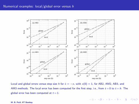
Numerical examples: local/global error versus h
10
10
10
10
−6
−2
−10
−14
100
10−4
10−8
10−12
10 10 10 10 10−4 −3 −2 −1 0
10 10 10 10 10−4 −3 −2 −1 010
10
10
10
−6
−2
−10
−14
10−2
10−6
10−10
10−14
(c) AB3 (d) AM3
globalglobal
locallocal
(a) AB2 (b) AM2
globalglobal
local local
10 10 10 10 10−4 −3 −2 −1 0
10 10 10 10 10−4 −3 −2 −1 0
step size (h) step size (h)
Err
or
Err
or
Err
or
Err
or
Local and global errors versus step size h for x = −x , with x(0) = 1, for AB2, AM2, AB3, and
AM3 methods. The local error has been computed for the first step, i.e., from t = 0 to t = h. The
global error has been computed at t = 1.
M. B. Patil, IIT Bombay

Numerical examples: comparison of methods
(a) (b)
(c) (d)
1.0
1.5
2.0
2.5
3.0x
exact
FE
1.0
1.5
2.0
2.5
3.0
x
exact
BE
1.0
1.5
2.0
2.5
3.0
0 1 2 3 4 5 6
x
t
exact
TRZ
1.0
1.5
2.0
2.5
3.0
0 1 2 3 4 5 6
x
t
exact
RK4
Exact and numerical solutions for x =sin(t), with x(0) = 1. (a) Forward Euler, (b) Backward Euler,
(c) Trapezoidal, and (d) Runge-Kutta (4th order).
M. B. Patil, IIT Bombay

Remarks on numerical examples
* For a method of order p,
- the local error is O(hp+1), i.e., if h is reduced by 10, the local error goesdown by 10p+1.
- the global error is O(hp), i.e., if h is reduced by 10, the global error goes
down by 10p .
* A higher-order method is more accurate and therefore allows larger time steps tobe taken.
* Should we always prefer a high-order method?NO. Need to worry about stability.
M. B. Patil, IIT Bombay
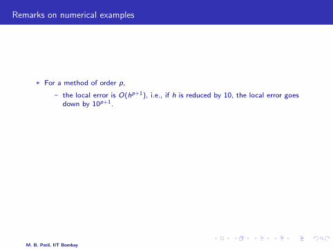
Remarks on numerical examples
* For a method of order p,
- the local error is O(hp+1), i.e., if h is reduced by 10, the local error goesdown by 10p+1.
- the global error is O(hp), i.e., if h is reduced by 10, the global error goes
down by 10p .
* A higher-order method is more accurate and therefore allows larger time steps tobe taken.
* Should we always prefer a high-order method?NO. Need to worry about stability.
M. B. Patil, IIT Bombay
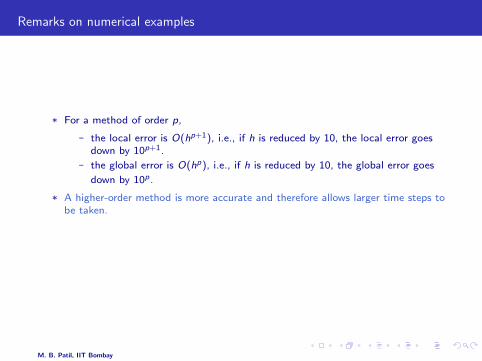
Remarks on numerical examples
* For a method of order p,
- the local error is O(hp+1), i.e., if h is reduced by 10, the local error goesdown by 10p+1.
- the global error is O(hp), i.e., if h is reduced by 10, the global error goes
down by 10p .
* A higher-order method is more accurate and therefore allows larger time steps tobe taken.
* Should we always prefer a high-order method?NO. Need to worry about stability.
M. B. Patil, IIT Bombay
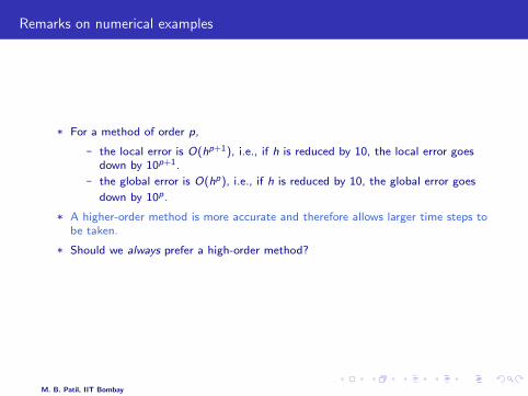
Remarks on numerical examples
* For a method of order p,
- the local error is O(hp+1), i.e., if h is reduced by 10, the local error goesdown by 10p+1.
- the global error is O(hp), i.e., if h is reduced by 10, the global error goes
down by 10p .
* A higher-order method is more accurate and therefore allows larger time steps tobe taken.
* Should we always prefer a high-order method?
NO. Need to worry about stability.
M. B. Patil, IIT Bombay

Remarks on numerical examples
* For a method of order p,
- the local error is O(hp+1), i.e., if h is reduced by 10, the local error goesdown by 10p+1.
- the global error is O(hp), i.e., if h is reduced by 10, the global error goes
down by 10p .
* A higher-order method is more accurate and therefore allows larger time steps tobe taken.
* Should we always prefer a high-order method?NO. Need to worry about stability.
M. B. Patil, IIT Bombay

Outline
* Introduction and problem definition
* Taylor series methods
* Runge-Kutta methods
* Specific multi-step methods
* Generalized multi-step methods
* Predictor-corrector methods
* Numerical results
* Stability of numerical methods
* Regions of stability
* Stiff equations
* Adaptive step size
* Miscellaneous topics
M. B. Patil, IIT Bombay

Stability of numerical methods for x = f (t, x)
* A numerical method generates a sequence of numbers, x1, x2, · · · toapproximate the actual values of the solution x(t1), x(t2), · · ·
* At a given time point tk , there is an error εk associated with the numericalsolution xk due to algorithmic and round-off errors.
* If the numerical method causes this error to get amplified in the subsequent timeintervals, |xn − x(tn)| can become indefinitely large as n→∞, and the methodis said to be unstable.
* Need to consider two cases:
- stability for small h (h→ 0)
- stability for large h
M. B. Patil, IIT Bombay
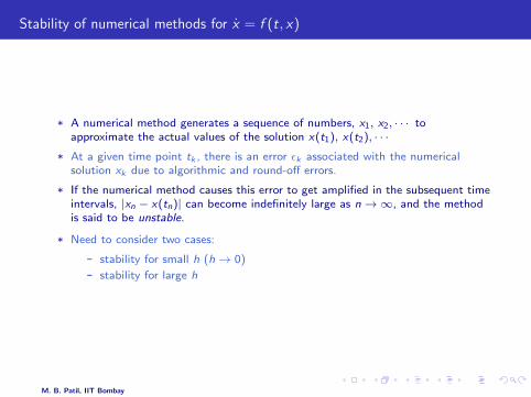
Stability of numerical methods for x = f (t, x)
* A numerical method generates a sequence of numbers, x1, x2, · · · toapproximate the actual values of the solution x(t1), x(t2), · · ·
* At a given time point tk , there is an error εk associated with the numericalsolution xk due to algorithmic and round-off errors.
* If the numerical method causes this error to get amplified in the subsequent timeintervals, |xn − x(tn)| can become indefinitely large as n→∞, and the methodis said to be unstable.
* Need to consider two cases:
- stability for small h (h→ 0)
- stability for large h
M. B. Patil, IIT Bombay
Stability for small h
* If small discrepancies due to a slightly different initial condition, algorithmicerrors, or round-off errors lead to correspondingly small changes in the computedsolution, then the method is said to be stable (for small h).
* A method that is not stable in the above sense is of no practical use becauseerrors are always introduced in solving an ODE numerically, which will cause anunstable method to “blow up” at some point of time.
* Runge-Kutta methods are stable.
* Linear multi-step methods (LMMs) can be unstable.
M. B. Patil, IIT Bombay
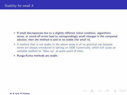
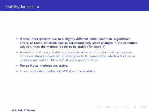
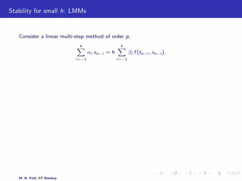
Stability for small h: LMMs
Consider a linear multi-step method of order p,
k∑i=−1
αi xn−i = hk∑
i=−1
βi f (tn−i , xn−i ) .
* Perturb the starting values; let ∆ be the largest perturbation.
* Perturb the recipe for evaluating xn+1 as,
k∑i=−1
αi xn−i = hk∑
i=−1
βi f (tn−i , xn−i ) + δn .
* If the difference between the original numerical solution (xorign ) and the numerical
solution of the perturbed problem (xnewn ) is such that,
max |xorign − xnew
n | ≤ S max(|∆|,max |δn|) ,then the method is called zero-stable or D-stable (after Dahlquist) or simplystable.
M. B. Patil, IIT Bombay
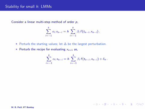
Stability for small h: LMMs
Consider a linear multi-step method of order p,
k∑i=−1
αi xn−i = hk∑
i=−1
βi f (tn−i , xn−i ) .
* Perturb the starting values; let ∆ be the largest perturbation.
* Perturb the recipe for evaluating xn+1 as,
k∑i=−1
αi xn−i = hk∑
i=−1
βi f (tn−i , xn−i ) + δn .
* If the difference between the original numerical solution (xorign ) and the numerical
solution of the perturbed problem (xnewn ) is such that,
max |xorign − xnew
n | ≤ S max(|∆|,max |δn|) ,then the method is called zero-stable or D-stable (after Dahlquist) or simplystable.
M. B. Patil, IIT Bombay
Stability for small h: LMMs
Consider two explicit second-order LMMs [2]:
(a) AB2: xn+1 = xn + h (1.5 fn − 0.5 fn−1)
(b) New2: xn+1 = 2.1 xn − 1.1 xn−1 + h (0.95 fn − 1.05 fn−1)
* Both of these methods satisfy the exactness constraints (discussed earlier).
* Apply the two methods to x =−x , x(0) = 1.
h=0.05
AB2
h=0.05
New2
h=0.01
New2
(c)(a)
numerical
exactexact
(b)
numerical
exactnumerical
3 0 1 2t
3 0 1 2t
0
1
x
0 1 2 3t
* New2 is unstable while AB2 is stable.
* Why are these two methods so different?
M. B. Patil, IIT Bombay
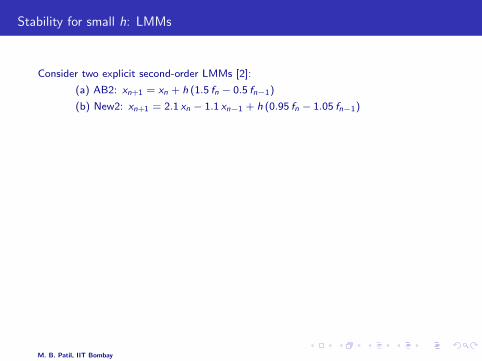
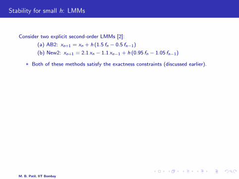
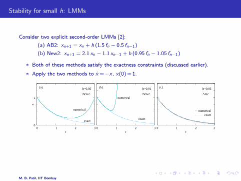
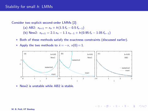
Difference equations: general solution
Consider a linear difference equation with constant (real) coefficients,
ak xm+k + ak−1xm+k−1 + · · ·+ a1xm+1 + a0xm = b . (11)
* The solution has two parts: (a) homogeneous, (b) particular.
* For the homogeneous part (i.e., b = 0), we seek a solution of the form x(h)i = z i ,
substitute it in Eq. 11, and obtain
zm[ak zk + ak−1zk−1 + · · ·+ a1z + a0
]= 0 . (12)
* Eq. 12 has the trivial solution z = 0, or
ak zk + ak−1zk−1 + · · ·+ a1z + a0 = 0 . (13)
* Eq. 13 is called the characteristic equation of the difference equation (Eq. 11).
M. B. Patil, IIT Bombay
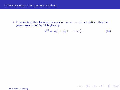
Difference equations: general solution
* If the roots of the characteristic equation, z1, z2, · · · , zk , are distinct, then thegeneral solution of Eq. 12 is given by
x(h)i = c1z i
1 + c2z i2 + · · ·+ ck z i
k . (14)
* If the roots are not distinct, then the general form for x(h)i gets modified. As an
example, if z1, z2, · · · , zl are identical, and the other roots are distinct, then x(h)i
is given by,
x(h)i = (c1 + c2n + · · ·+ cl n
l−1)z i1 + cl+1z i
l+1 + · · ·+ ck z ik . (15)
* The complete solution of Eq. 11 is then given by,
xi = x(h)i + x
(p)i , (16)
where x(p)i is a particular solution. The constants c1, c2, etc. can be determined
from the initial condition(s), i.e., the starting values in the sequence xi.
M. B. Patil, IIT Bombay
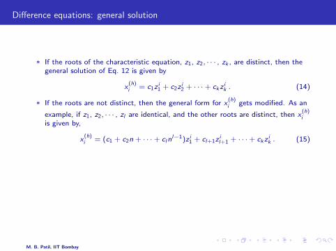
Difference equations: general solution
* If the roots of the characteristic equation, z1, z2, · · · , zk , are distinct, then thegeneral solution of Eq. 12 is given by
x(h)i = c1z i
1 + c2z i2 + · · ·+ ck z i
k . (14)
* If the roots are not distinct, then the general form for x(h)i gets modified. As an
example, if z1, z2, · · · , zl are identical, and the other roots are distinct, then x(h)i
is given by,
x(h)i = (c1 + c2n + · · ·+ cl n
l−1)z i1 + cl+1z i
l+1 + · · ·+ ck z ik . (15)
* The complete solution of Eq. 11 is then given by,
xi = x(h)i + x
(p)i , (16)
where x(p)i is a particular solution. The constants c1, c2, etc. can be determined
from the initial condition(s), i.e., the starting values in the sequence xi.
M. B. Patil, IIT Bombay
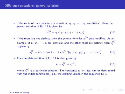
Difference equations: general solution
* If the roots of the characteristic equation, z1, z2, · · · , zk , are distinct, then thegeneral solution of Eq. 12 is given by
x(h)i = c1z i
1 + c2z i2 + · · ·+ ck z i
k . (14)
* If the roots are not distinct, then the general form for x(h)i gets modified. As an
example, if z1, z2, · · · , zl are identical, and the other roots are distinct, then x(h)i
is given by,
x(h)i = (c1 + c2n + · · ·+ cl n
l−1)z i1 + cl+1z i
l+1 + · · ·+ ck z ik . (15)
* The complete solution of Eq. 11 is then given by,
xi = x(h)i + x
(p)i , (16)
where x(p)i is a particular solution. The constants c1, c2, etc. can be determined
from the initial condition(s), i.e., the starting values in the sequence xi.
M. B. Patil, IIT Bombay
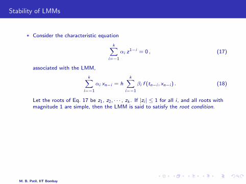
Stability of LMMs
* Consider the characteristic equation
k∑i=−1
αi z1−i = 0 , (17)
associated with the LMM,
k∑i=−1
αi xn−i = hk∑
i=−1
βi f (tn−i , xn−i ) . (18)
Let the roots of Eq. 17 be z1, z2, · · · , zk . If |zi | ≤ 1 for all i , and all roots withmagnitude 1 are simple, then the LMM is said to satisfy the root condition.
* If an LMM satisfies the root condition, and if the only root of the associatedcharacteristic equation with magnitude one is equal to 1, then the LMM is saidto be strongly stable.
* If an LMM satisfies the root condition, and if more than one (distinct) roots ofthe associated characteristic equation have magnitude one, then the LMM issaid to be weakly stable.
* If an LMM does not satisfy the root condition, it is said to be unstable.
M. B. Patil, IIT Bombay
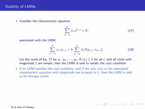
Stability of LMMs
* Consider the characteristic equation
k∑i=−1
αi z1−i = 0 , (17)
associated with the LMM,
k∑i=−1
αi xn−i = hk∑
i=−1
βi f (tn−i , xn−i ) . (18)
Let the roots of Eq. 17 be z1, z2, · · · , zk . If |zi | ≤ 1 for all i , and all roots withmagnitude 1 are simple, then the LMM is said to satisfy the root condition.
* If an LMM satisfies the root condition, and if the only root of the associatedcharacteristic equation with magnitude one is equal to 1, then the LMM is saidto be strongly stable.
* If an LMM satisfies the root condition, and if more than one (distinct) roots ofthe associated characteristic equation have magnitude one, then the LMM issaid to be weakly stable.
* If an LMM does not satisfy the root condition, it is said to be unstable.
M. B. Patil, IIT Bombay
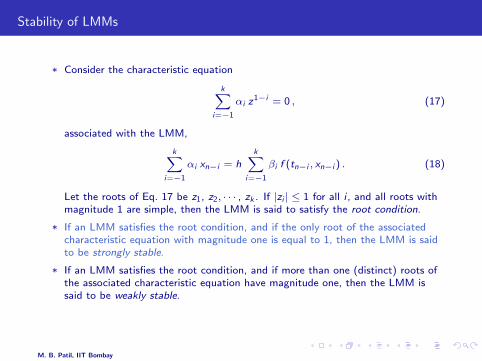
Stability of LMMs
* Consider the characteristic equation
k∑i=−1
αi z1−i = 0 , (17)
associated with the LMM,
k∑i=−1
αi xn−i = hk∑
i=−1
βi f (tn−i , xn−i ) . (18)
Let the roots of Eq. 17 be z1, z2, · · · , zk . If |zi | ≤ 1 for all i , and all roots withmagnitude 1 are simple, then the LMM is said to satisfy the root condition.
* If an LMM satisfies the root condition, and if the only root of the associatedcharacteristic equation with magnitude one is equal to 1, then the LMM is saidto be strongly stable.
* If an LMM satisfies the root condition, and if more than one (distinct) roots ofthe associated characteristic equation have magnitude one, then the LMM issaid to be weakly stable.
* If an LMM does not satisfy the root condition, it is said to be unstable.
M. B. Patil, IIT Bombay
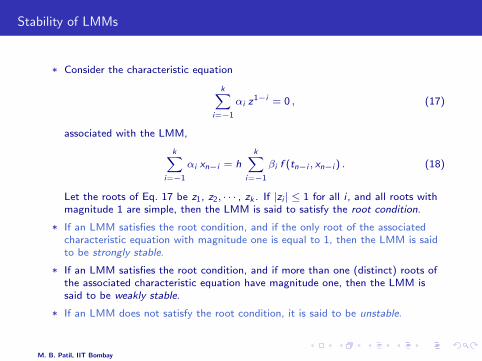
Stability of LMMs
* Consider the characteristic equation
k∑i=−1
αi z1−i = 0 , (17)
associated with the LMM,
k∑i=−1
αi xn−i = hk∑
i=−1
βi f (tn−i , xn−i ) . (18)
Let the roots of Eq. 17 be z1, z2, · · · , zk . If |zi | ≤ 1 for all i , and all roots withmagnitude 1 are simple, then the LMM is said to satisfy the root condition.
* If an LMM satisfies the root condition, and if the only root of the associatedcharacteristic equation with magnitude one is equal to 1, then the LMM is saidto be strongly stable.
* If an LMM satisfies the root condition, and if more than one (distinct) roots ofthe associated characteristic equation have magnitude one, then the LMM issaid to be weakly stable.
* If an LMM does not satisfy the root condition, it is said to be unstable.
M. B. Patil, IIT Bombay
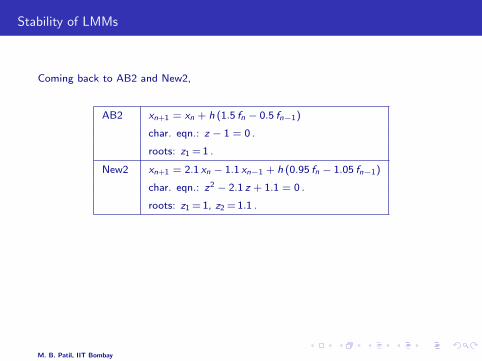
Stability of LMMs
Coming back to AB2 and New2,
AB2 xn+1 = xn + h (1.5 fn − 0.5 fn−1)
char. eqn.: z − 1 = 0 .
roots: z1 = 1 .
New2 xn+1 = 2.1 xn − 1.1 xn−1 + h (0.95 fn − 1.05 fn−1)
char. eqn.: z2 − 2.1 z + 1.1 = 0 .
roots: z1 = 1, z2 = 1.1 .
* AB2 satisfies the root condition; New2 does not.
* For the New2 method, the general solution, c1zn1 + c2zn
2 , can grow indefinitelysince |z2| > 1.
* Even if c2 is forced to be zero because of initial conditions, numerical errors canmake it non-zero.
M. B. Patil, IIT Bombay
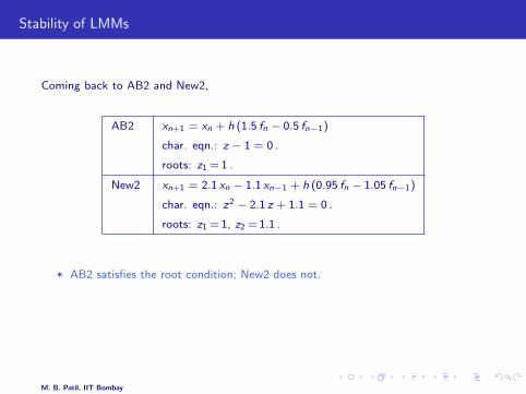
Stability of LMMs
Coming back to AB2 and New2,
AB2 xn+1 = xn + h (1.5 fn − 0.5 fn−1)
char. eqn.: z − 1 = 0 .
roots: z1 = 1 .
New2 xn+1 = 2.1 xn − 1.1 xn−1 + h (0.95 fn − 1.05 fn−1)
char. eqn.: z2 − 2.1 z + 1.1 = 0 .
roots: z1 = 1, z2 = 1.1 .
* AB2 satisfies the root condition; New2 does not.
* For the New2 method, the general solution, c1zn1 + c2zn
2 , can grow indefinitelysince |z2| > 1.
* Even if c2 is forced to be zero because of initial conditions, numerical errors canmake it non-zero.
M. B. Patil, IIT Bombay
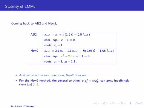
Stability of LMMs
Coming back to AB2 and New2,
AB2 xn+1 = xn + h (1.5 fn − 0.5 fn−1)
char. eqn.: z − 1 = 0 .
roots: z1 = 1 .
New2 xn+1 = 2.1 xn − 1.1 xn−1 + h (0.95 fn − 1.05 fn−1)
char. eqn.: z2 − 2.1 z + 1.1 = 0 .
roots: z1 = 1, z2 = 1.1 .
* AB2 satisfies the root condition; New2 does not.
* For the New2 method, the general solution, c1zn1 + c2zn
2 , can grow indefinitelysince |z2| > 1.
* Even if c2 is forced to be zero because of initial conditions, numerical errors canmake it non-zero.
M. B. Patil, IIT Bombay

Stability for large h
* A numerical method that is unstable even for small values of h (e.g., the “New2”method seen earlier) is practically useless since it is unstable for any problem.
* A method that is stable for small h (e.g., the AB2 method) may still be unstablein a different sense, viz., unstable if h exceeds a certain value, say, hmax.
* hmax would depend on the ODE being solved. Generally, it is determined for thetest equation,
x = λx , x(0) = 1 , (19)
where λ is a constant, a complex number in general. Eq. 19 is representative ofseveral problems of practical importance, such as RC circuits.
M. B. Patil, IIT Bombay
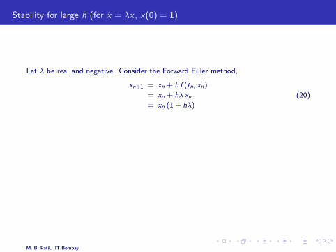
Stability for large h (for x = λx , x(0) = 1)
Let λ be real and negative. Consider the Forward Euler method,
xn+1 = xn + h f (tn, xn)
= xn + hλ xn
= xn (1 + hλ)
(20)
The characteristic equation for this difference equation is,
z − (1 + hλ) = 0 , (21)
for which the general solution is given by,
xi = c1 z i1
= (1 + hλ)i .(22)
(c1 = 1 is required to satisfy the initial condition, x0 = 1.)
M. B. Patil, IIT Bombay
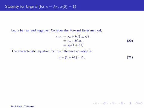
Stability for large h (for x = λx , x(0) = 1)
Let λ be real and negative. Consider the Forward Euler method,
xn+1 = xn + h f (tn, xn)
= xn + hλ xn
= xn (1 + hλ)
(20)
The characteristic equation for this difference equation is,
z − (1 + hλ) = 0 , (21)
for which the general solution is given by,
xi = c1 z i1
= (1 + hλ)i .(22)
(c1 = 1 is required to satisfy the initial condition, x0 = 1.)
M. B. Patil, IIT Bombay
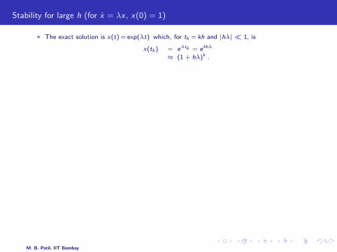
Stability for large h (for x = λx , x(0) = 1)
* The exact solution is x(t) = exp(λt) which, for tk = kh and |hλ| 1, is
x(tk ) = eλtk = ekhλ
≈ (1 + hλ)k .
* Comparing with the numerical solution,
xk = (1 + hλ)k,
we see that the numerical solution will approximate the true solution if hλ is small.
* As h is increased, z1 = 1 + hλ decreases (since λ < 0), and for hλ=−2, z1 becomes equal
to -1 (see figure). Beyond this point, |z1| > 1, and the numerical solution (xk = c1 zk1 )
grows indefinitely with k ⇒ instability.
FE
−1.5
−1.0
−0.5
0.0
0.5
1.0
−2.5 −2.0 −1.5 −1.0 −0.5 0.0
hλ
ehλ
z1
M. B. Patil, IIT Bombay
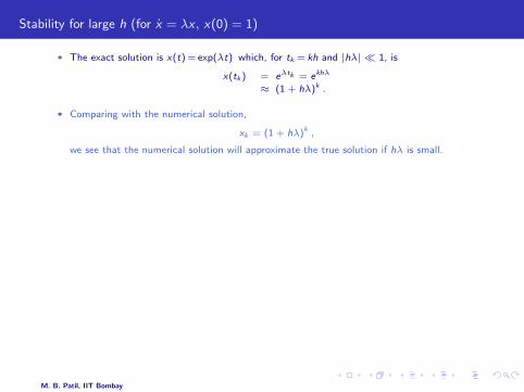
Stability for large h (for x = λx , x(0) = 1)
* The exact solution is x(t) = exp(λt) which, for tk = kh and |hλ| 1, is
x(tk ) = eλtk = ekhλ
≈ (1 + hλ)k .
* Comparing with the numerical solution,
xk = (1 + hλ)k,
we see that the numerical solution will approximate the true solution if hλ is small.
* As h is increased, z1 = 1 + hλ decreases (since λ < 0), and for hλ=−2, z1 becomes equal
to -1 (see figure). Beyond this point, |z1| > 1, and the numerical solution (xk = c1 zk1 )
grows indefinitely with k ⇒ instability.
FE
−1.5
−1.0
−0.5
0.0
0.5
1.0
−2.5 −2.0 −1.5 −1.0 −0.5 0.0
hλ
ehλ
z1
M. B. Patil, IIT Bombay
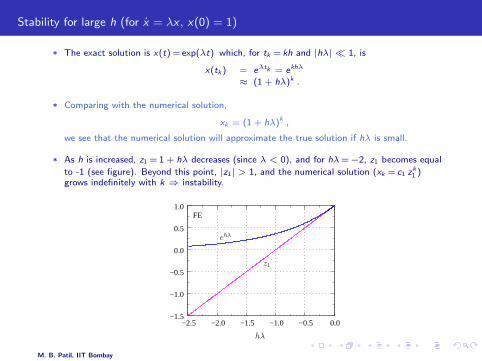
Stability for large h (for x = λx , x(0) = 1)
* The exact solution is x(t) = exp(λt) which, for tk = kh and |hλ| 1, is
x(tk ) = eλtk = ekhλ
≈ (1 + hλ)k .
* Comparing with the numerical solution,
xk = (1 + hλ)k,
we see that the numerical solution will approximate the true solution if hλ is small.
* As h is increased, z1 = 1 + hλ decreases (since λ < 0), and for hλ=−2, z1 becomes equal
to -1 (see figure). Beyond this point, |z1| > 1, and the numerical solution (xk = c1 zk1 )
grows indefinitely with k ⇒ instability.
FE
−1.5
−1.0
−0.5
0.0
0.5
1.0
−2.5 −2.0 −1.5 −1.0 −0.5 0.0
hλ
ehλ
z1
M. B. Patil, IIT Bombay

Stability for large h (for x = λx , x(0) = 1)
Consider the second-order Adams-Bashforth method. The difference equation is,
xn+1 = xn + hλ
[3
2xn −
1
2xn−1
].
The characteristic equation for this case is,
z2 −(
1 +3hλ
2
)z +
(hλ
2
)= 0 ,
with the roots,
z1,2 =1
2
(
1 +3hλ
2
)±
√(1 +
3hλ
2
)2
− 2hλ
,
and the general solution,
xi = c1z i1 + c2z i
2 .
M. B. Patil, IIT Bombay
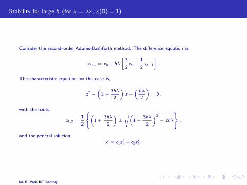
Stability for large h (for x = λx , x(0) = 1)
Consider the second-order Adams-Bashforth method. The difference equation is,
xn+1 = xn + hλ
[3
2xn −
1
2xn−1
].
The characteristic equation for this case is,
z2 −(
1 +3hλ
2
)z +
(hλ
2
)= 0 ,
with the roots,
z1,2 =1
2
(
1 +3hλ
2
)±
√(1 +
3hλ
2
)2
− 2hλ
,
and the general solution,
xi = c1z i1 + c2z i
2 .
M. B. Patil, IIT Bombay

Stability for large h (AB2 method for x = λx , x(0) = 1)
AB2
−1.5
−1.0
−0.5
0.0
0.5
1.0
−2.5 −2.0 −1.5 −1.0 −0.5 0.0
hλ
ehλ
z1
z2
* For small values of hλ, z1 represents ehλ more closely than in the FE method, aswe would expect from a second-order method.
* What is of concern, from the stability angle, is the other root z2 which starts offat zero, but becomes greater than one in magnitude at hλ=−1, thus leading toinstability.
* This root is not required to represent ehλ, and in that sense, it is a parasitic orspurious root. In contrast, the root z1, which approximates ehλ, is called theprincipal root.
M. B. Patil, IIT Bombay

Stability for large h: AB and AM methods for x = λx , λ < 0
(a) (b)Adams−Moulton Adams−Bashforth
p=1
p=2
p=3
p=4
p=5
p=6
p=1
p=2
p=3
p=4
p=5
p=6
−7 −6 −5 −4 −3 −2 −1 0 1 −2.5 −2 −1.5 −1 −0.5 0 0.5
hλhλ
* The AM methods, for the same order, are more stable than the AB methods.
* The AM methods of order 1 and 2 (the BE and TRZ methods) are stable for allvalues of hλ.
* As the order increases, the range of stability becomes smaller for both AB andAM methods. This explains why higher-order methods are not used in circuitsimulation.
M. B. Patil, IIT Bombay
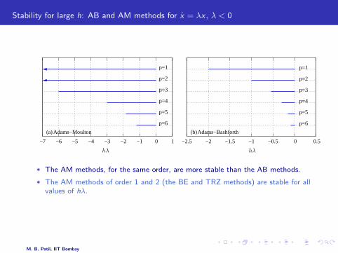
Stability for large h: AB and AM methods for x = λx , λ < 0
(a) (b)Adams−Moulton Adams−Bashforth
p=1
p=2
p=3
p=4
p=5
p=6
p=1
p=2
p=3
p=4
p=5
p=6
−7 −6 −5 −4 −3 −2 −1 0 1 −2.5 −2 −1.5 −1 −0.5 0 0.5
hλhλ
* The AM methods, for the same order, are more stable than the AB methods.
* The AM methods of order 1 and 2 (the BE and TRZ methods) are stable for allvalues of hλ.
* As the order increases, the range of stability becomes smaller for both AB andAM methods. This explains why higher-order methods are not used in circuitsimulation.
M. B. Patil, IIT Bombay
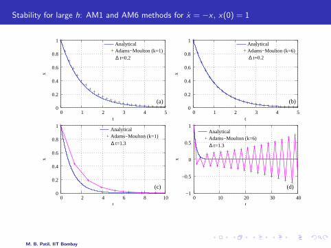
Stability for large h: AM1 and AM6 methods for x = −x , x(0) = 1
t=0.2∆ t=0.2∆
(a) (b)
∆ t=1.3∆ t=1.3
(c) (d)
0
0.2
0.4
0.6
0.8
1
0 1 2 3 4 5
x
t
AnalyticalAdams−Moulton (k=1)
0
0.2
0.4
0.6
0.8
1
0 1 2 3 4 5
x
t
Adams−Moulton (k=6)Analytical
−1
−0.5
0
0.5
1
0 10 20 30 40
x
t
AnalyticalAdams−Moulton (k=6)
0
0.2
0.4
0.6
0.8
1
0 2 4 6 8 10
x
t
AnalyticalAdams−Moulton (k=1)
* AM6 is more accurate than AM1 (upper figures).
* For ∆t = 1.3, AM1 is stable, but AM6 is not (lower figures).
M. B. Patil, IIT Bombay
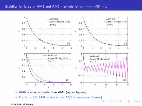
Stability for large h: AM1 and AM6 methods for x = −x , x(0) = 1
t=0.2∆ t=0.2∆
(a) (b)
∆ t=1.3∆ t=1.3
(c) (d)
0
0.2
0.4
0.6
0.8
1
0 1 2 3 4 5
x
t
AnalyticalAdams−Moulton (k=1)
0
0.2
0.4
0.6
0.8
1
0 1 2 3 4 5
x
t
Adams−Moulton (k=6)Analytical
−1
−0.5
0
0.5
1
0 10 20 30 40
x
t
AnalyticalAdams−Moulton (k=6)
0
0.2
0.4
0.6
0.8
1
0 2 4 6 8 10
x
t
AnalyticalAdams−Moulton (k=1)
* AM6 is more accurate than AM1 (upper figures).
* For ∆t = 1.3, AM1 is stable, but AM6 is not (lower figures).
M. B. Patil, IIT Bombay

Stability for large h (x = λ x , complex λ)
Consider the 2× 2 system of ODEs, x=Ax, which may be written in the expandedform,
x1 = a11x1 + a12x2 ,
x2 = a21x1 + a22x2 ,(23)
with x1(0) = x01 and x2(0) = x0
2 .
Let λ1, λ2 be the eigenvalues (assumed to be distinct) of A, and S1, S2 be thecorresponding eigenvectors.
Eq. 23 can be re-written in a diagonalized form,
y1 = λ1y1 ,
y2 = λ2y2 .(24)
The new variables y1 and y2 are given by,[y1
y2
]= [S1 S2]
[x1
x2
]. (25)
Solving the system of ODEs, Eq. 23, is thus equivalent to solving two separate ODEs.Since λ1, λ2 are generally complex, we are interested in solving x = λx when λ iscomplex.
M. B. Patil, IIT Bombay
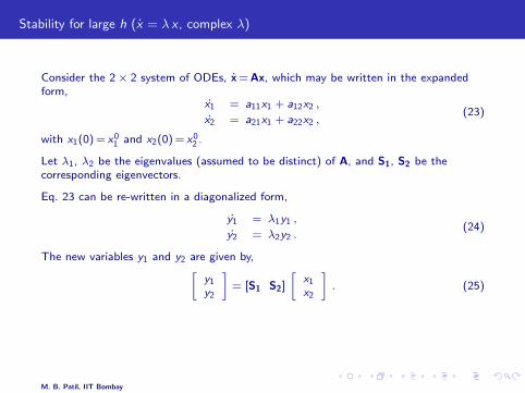
Stability for large h (x = λ x , complex λ)
Consider the 2× 2 system of ODEs, x=Ax, which may be written in the expandedform,
x1 = a11x1 + a12x2 ,
x2 = a21x1 + a22x2 ,(23)
with x1(0) = x01 and x2(0) = x0
2 .
Let λ1, λ2 be the eigenvalues (assumed to be distinct) of A, and S1, S2 be thecorresponding eigenvectors.
Eq. 23 can be re-written in a diagonalized form,
y1 = λ1y1 ,
y2 = λ2y2 .(24)
The new variables y1 and y2 are given by,[y1
y2
]= [S1 S2]
[x1
x2
]. (25)
Solving the system of ODEs, Eq. 23, is thus equivalent to solving two separate ODEs.Since λ1, λ2 are generally complex, we are interested in solving x = λx when λ iscomplex.
M. B. Patil, IIT Bombay
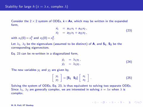
Stability for large h (x = λ x , complex λ)
Consider the 2× 2 system of ODEs, x=Ax, which may be written in the expandedform,
x1 = a11x1 + a12x2 ,
x2 = a21x1 + a22x2 ,(23)
with x1(0) = x01 and x2(0) = x0
2 .
Let λ1, λ2 be the eigenvalues (assumed to be distinct) of A, and S1, S2 be thecorresponding eigenvectors.
Eq. 23 can be re-written in a diagonalized form,
y1 = λ1y1 ,
y2 = λ2y2 .(24)
The new variables y1 and y2 are given by,[y1
y2
]= [S1 S2]
[x1
x2
]. (25)
Solving the system of ODEs, Eq. 23, is thus equivalent to solving two separate ODEs.Since λ1, λ2 are generally complex, we are interested in solving x = λx when λ iscomplex.
M. B. Patil, IIT Bombay

Outline
* Introduction and problem definition
* Taylor series methods
* Runge-Kutta methods
* Specific multi-step methods
* Generalized multi-step methods
* Predictor-corrector methods
* Numerical results
* Stability of numerical methods
* Regions of stability
* Stiff equations
* Adaptive step size
* Miscellaneous topics
M. B. Patil, IIT Bombay
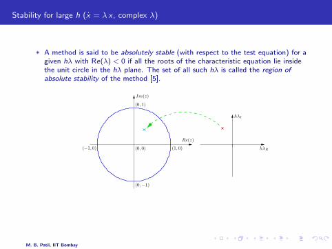
Stability for large h (x = λ x , complex λ)
* A method is said to be absolutely stable (with respect to the test equation) for agiven hλ with Re(λ) < 0 if all the roots of the characteristic equation lie insidethe unit circle in the hλ plane. The set of all such hλ is called the region ofabsolute stability of the method [5].
(−1, 0) (0, 0)
(0,−1)
(1, 0)
Re(z)
(0, 1)
hλR
hλI
Im(z)
* Methods that are stable for all λ with Re(λ) < 0 are called A-stable.
M. B. Patil, IIT Bombay

Region of stability for AB methods
p=2 p=3p=1
p=4 p=5 p=6−1
−1−2 0
1
hλI
hλR
hλI
hλR
hλR hλR
hλR
hλR
hλI
hλI hλI hλI
M. B. Patil, IIT Bombay
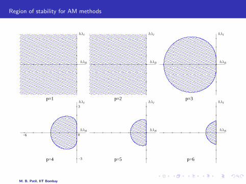
Region of stability for AM methods
p=1
p=4
3
−3
−6 0
p=3p=2
p=5 p=6
hλR
hλR
hλI
hλI
hλR
hλI
hλR
hλI
hλI
hλR
hλI
hλR
M. B. Patil, IIT Bombay
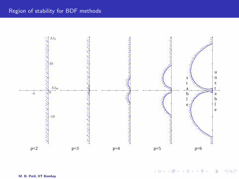
Region of stability for BDF methods
stable
unstable
p=3 p=4 p=5 p=6p=2
-4
hλI
hλR
-10
10
0
M. B. Patil, IIT Bombay

Stability for large h (x = λ x , complex λ)
* The AM1 (Backward Euler), AM2 (Trapezoidal), and second-order BDFmethods are A-stable; other methods are conditionally stable.
* The region of absolute stability for each method shrinks significantly as the orderincreases.
* For purely real values of λ, the BDF methods (up to order six) areunconditionally stable, while the AB and AM (except AM1 and AM2) methodsare conditionally stable.
* Stability conditions impose restrictions on the choice of methods for circuitsimulation.
M. B. Patil, IIT Bombay
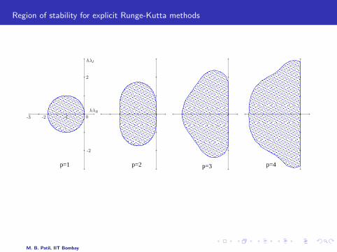
Region of stability for explicit Runge-Kutta methods
p=1 p=2 p=3 p=4
hλI
hλR
-2
-2 0
2
-3 -1
* Explicit Runge-Kutta methods are conditionally stable.
* On the other hand, implicit Runge-Kutta methods are A-stable [4].
M. B. Patil, IIT Bombay
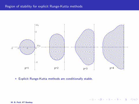
Region of stability for explicit Runge-Kutta methods
p=1 p=2 p=3 p=4
hλI
hλR
-2
-2 0
2
-3 -1
* Explicit Runge-Kutta methods are conditionally stable.
* On the other hand, implicit Runge-Kutta methods are A-stable [4].
M. B. Patil, IIT Bombay
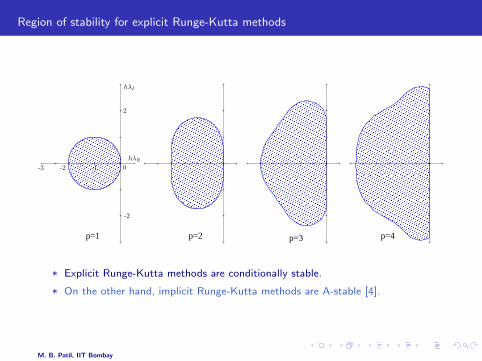
Region of stability for explicit Runge-Kutta methods
p=1 p=2 p=3 p=4
hλI
hλR
-2
-2 0
2
-3 -1
* Explicit Runge-Kutta methods are conditionally stable.
* On the other hand, implicit Runge-Kutta methods are A-stable [4].
M. B. Patil, IIT Bombay

Outline
* Introduction and problem definition
* Taylor series methods
* Runge-Kutta methods
* Specific multi-step methods
* Generalized multi-step methods
* Predictor-corrector methods
* Numerical results
* Stability of numerical methods
* Regions of stability
* Stiff equations
* Adaptive step size
* Miscellaneous topics
M. B. Patil, IIT Bombay

Stiff equations
Consider the 2× 2 system of ODEs,
x1 = a11x1 + a12x2 ,
x2 = a21x1 + a22x2 .(26)
* If the magnitudes of the eigenvalues λ1 and λ2 of the A matrix are significantlydifferent, the system of ODEs is said to be stiff. (The same idea applies to largersystems as well.)
* There are several physical examples of stiff systems, such as motion of massesconnected by springs, chemical reactions involving several reactants, andelectrical circuits.
* Stiff equations present a challenge because they involve vastly different timeconstants. In some cases, it is important for the numerical method to be able toresolve transients on a time scale corresponding to the smallest time constant.
M. B. Patil, IIT Bombay

Stiff equations: RC circuit example
V0C C1 2
R R21
0
V1 V2
dV1
dt=
(−1
C1
)(1
R1+
1
R2
)V1 +
(1
C1R2
)V2 +
(V0
C1R1
),
dV2
dt=
(1
C2R2
)V1 −
(1
C2R2
)V2 .
(27)
* This is a coupled system of ODEs (see Eq. 26).
* For R1 = 0.5 Ω, R2 = 5 Ω, C1 = 0.01 F , C2 = 1 F ,the eigenvalues are, λ1 =−0.182 s−1, λ2 =−220 s−1,and the time constants are τ1 = 5.5 s, τ2 = 0.0045 s.
* Note that τ1 ≈ 1000× τ2.
M. B. Patil, IIT Bombay
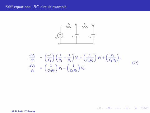
Stiff equations: RC circuit example
V0C C1 2
R R21
0
V1 V2
dV1
dt=
(−1
C1
)(1
R1+
1
R2
)V1 +
(1
C1R2
)V2 +
(V0
C1R1
),
dV2
dt=
(1
C2R2
)V1 −
(1
C2R2
)V2 .
(27)
* This is a coupled system of ODEs (see Eq. 26).
* For R1 = 0.5 Ω, R2 = 5 Ω, C1 = 0.01 F , C2 = 1 F ,the eigenvalues are, λ1 =−0.182 s−1, λ2 =−220 s−1,and the time constants are τ1 = 5.5 s, τ2 = 0.0045 s.
* Note that τ1 ≈ 1000× τ2.
M. B. Patil, IIT Bombay
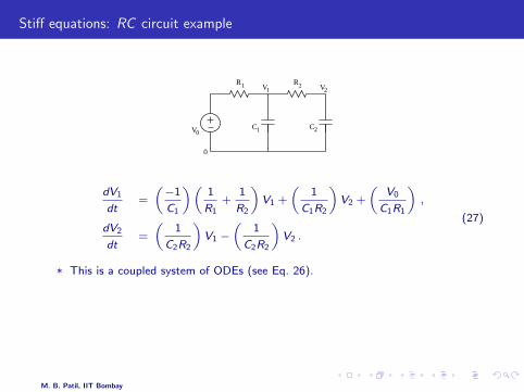
Stiff equations: RC circuit example
V0C C1 2
R R21
0
V1 V2
dV1
dt=
(−1
C1
)(1
R1+
1
R2
)V1 +
(1
C1R2
)V2 +
(V0
C1R1
),
dV2
dt=
(1
C2R2
)V1 −
(1
C2R2
)V2 .
(27)
* This is a coupled system of ODEs (see Eq. 26).
* For R1 = 0.5 Ω, R2 = 5 Ω, C1 = 0.01 F , C2 = 1 F ,the eigenvalues are, λ1 =−0.182 s−1, λ2 =−220 s−1,and the time constants are τ1 = 5.5 s, τ2 = 0.0045 s.
* Note that τ1 ≈ 1000× τ2.
M. B. Patil, IIT Bombay

Stiff equations: RC circuit example
V 1
V 1
time (sec)time (sec)
(a) (b)Analytical Analytical 0
2
4
6
8
10
−5 0 5 10 15 20 25 0
2
4
6
8
10
0 0.02 0.04 0.06 0.08 0.1
* The currents and voltages in the circuit are given by the general form,
x(t) = Ae−t/τ1 + Be−t/τ2 + C . (28)
* Two transients can be seen in (a) – an initial fast transient due to τ2, followedby a slow transient due to τ1.
* An expanded view of the fast transient is shown in (b).
M. B. Patil, IIT Bombay
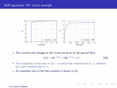
Stiff equations: RC circuit example
V 1
V 1
time (sec)time (sec)
(a) (b)Analytical Analytical 0
2
4
6
8
10
−5 0 5 10 15 20 25 0
2
4
6
8
10
0 0.02 0.04 0.06 0.08 0.1
* The currents and voltages in the circuit are given by the general form,
x(t) = Ae−t/τ1 + Be−t/τ2 + C . (28)
* Two transients can be seen in (a) – an initial fast transient due to τ2, followedby a slow transient due to τ1.
* An expanded view of the fast transient is shown in (b).
M. B. Patil, IIT Bombay
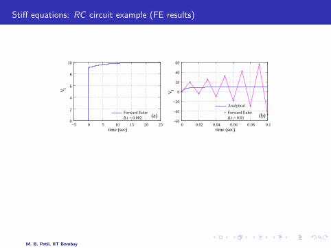
Stiff equations: RC circuit example (FE results)
V 1V 1
∆ t = 0.01∆ t = 0.002
time (sec)time (sec)
(a) (b)Forward Euler
Analytical
Forward Euler
0
2
4
6
8
10
−5 0 5 10 15 20 25 −60
−40
−20
0
20
40
60
0 0.02 0.04 0.06 0.08 0.1
* For ∆t = 0.002 s, Forward Euler results are acceptable.
* For ∆t = 0.01 s, which is large than 2 τ2 but much smaller than τ1, the ForwardEuler method is unstable.
* To prevent the unstable behaviour, a small time step is required throughout, i.e.,even after the fast transient has vanished ⇒ extremely inefficient simulation.
M. B. Patil, IIT Bombay
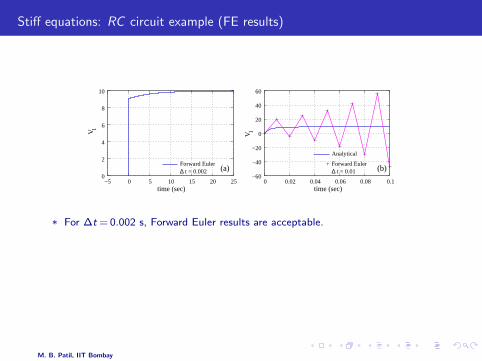
Stiff equations: RC circuit example (FE results)
V 1V 1
∆ t = 0.01∆ t = 0.002
time (sec)time (sec)
(a) (b)Forward Euler
Analytical
Forward Euler
0
2
4
6
8
10
−5 0 5 10 15 20 25 −60
−40
−20
0
20
40
60
0 0.02 0.04 0.06 0.08 0.1
* For ∆t = 0.002 s, Forward Euler results are acceptable.
* For ∆t = 0.01 s, which is large than 2 τ2 but much smaller than τ1, the ForwardEuler method is unstable.
* To prevent the unstable behaviour, a small time step is required throughout, i.e.,even after the fast transient has vanished ⇒ extremely inefficient simulation.
M. B. Patil, IIT Bombay
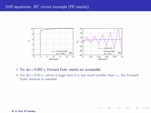
Stiff equations: RC circuit example (FE results)
V 1V 1
∆ t = 0.01∆ t = 0.002
time (sec)time (sec)
(a) (b)Forward Euler
Analytical
Forward Euler
0
2
4
6
8
10
−5 0 5 10 15 20 25 −60
−40
−20
0
20
40
60
0 0.02 0.04 0.06 0.08 0.1
* For ∆t = 0.002 s, Forward Euler results are acceptable.
* For ∆t = 0.01 s, which is large than 2 τ2 but much smaller than τ1, the ForwardEuler method is unstable.
* To prevent the unstable behaviour, a small time step is required throughout, i.e.,even after the fast transient has vanished ⇒ extremely inefficient simulation.
M. B. Patil, IIT Bombay
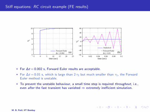
Stiff equations: RC circuit example (FE results)
V 1V 1
∆ t = 0.01∆ t = 0.002
time (sec)time (sec)
(a) (b)Forward Euler
Analytical
Forward Euler
0
2
4
6
8
10
−5 0 5 10 15 20 25 −60
−40
−20
0
20
40
60
0 0.02 0.04 0.06 0.08 0.1
* For ∆t = 0.002 s, Forward Euler results are acceptable.
* For ∆t = 0.01 s, which is large than 2 τ2 but much smaller than τ1, the ForwardEuler method is unstable.
* To prevent the unstable behaviour, a small time step is required throughout, i.e.,even after the fast transient has vanished ⇒ extremely inefficient simulation.
M. B. Patil, IIT Bombay
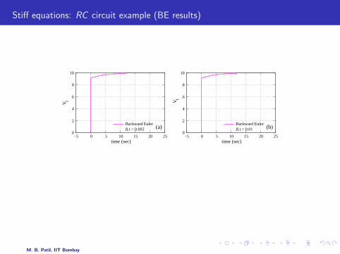
Stiff equations: RC circuit example (BE results)
V 1
V 1
∆ t = 0.01∆ t = 0.002
time (sec)time (sec)
(a) (b)Backward EulerBackward Euler
0
2
4
6
8
10
−5 0 5 10 15 20 25 0
2
4
6
8
10
−5 0 5 10 15 20 25
* The Backward Euler method is stable for For ∆t = 0.01 s as well, which isexpected from an A-stable method.
* The BE method allows much larger time steps than the FE method.
M. B. Patil, IIT Bombay
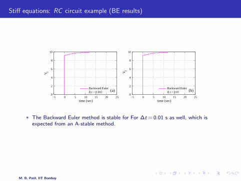
Stiff equations: RC circuit example (BE results)
V 1
V 1
∆ t = 0.01∆ t = 0.002
time (sec)time (sec)
(a) (b)Backward EulerBackward Euler
0
2
4
6
8
10
−5 0 5 10 15 20 25 0
2
4
6
8
10
−5 0 5 10 15 20 25
* The Backward Euler method is stable for For ∆t = 0.01 s as well, which isexpected from an A-stable method.
* The BE method allows much larger time steps than the FE method.
M. B. Patil, IIT Bombay
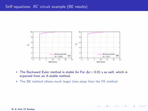
Stiff equations: RC circuit example (BE results)
V 1
V 1
∆ t = 0.01∆ t = 0.002
time (sec)time (sec)
(a) (b)Backward EulerBackward Euler
0
2
4
6
8
10
−5 0 5 10 15 20 25 0
2
4
6
8
10
−5 0 5 10 15 20 25
* The Backward Euler method is stable for For ∆t = 0.01 s as well, which isexpected from an A-stable method.
* The BE method allows much larger time steps than the FE method.
M. B. Patil, IIT Bombay

Stiff equations: RC circuit example (BE results)
V 1∆ t = 0.01Backward Euler
Analytical
time (sec)
0
2
4
6
8
10
0 0.02 0.04 0.06 0.08 0.1
* Although the BE method with ∆t = 0.01 s works well for the slow transient, itdoes not capture the fast transient accurately, as shown in this expanded view.
* In practice, the time step is made small when things are changing rapidly, andlarge otherwise. This strategy makes the simulation faster without compromisingon accuracy.
M. B. Patil, IIT Bombay
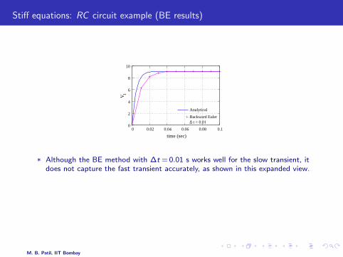
Stiff equations: RC circuit example (BE results)
V 1∆ t = 0.01Backward Euler
Analytical
time (sec)
0
2
4
6
8
10
0 0.02 0.04 0.06 0.08 0.1
* Although the BE method with ∆t = 0.01 s works well for the slow transient, itdoes not capture the fast transient accurately, as shown in this expanded view.
* In practice, the time step is made small when things are changing rapidly, andlarge otherwise. This strategy makes the simulation faster without compromisingon accuracy.
M. B. Patil, IIT Bombay
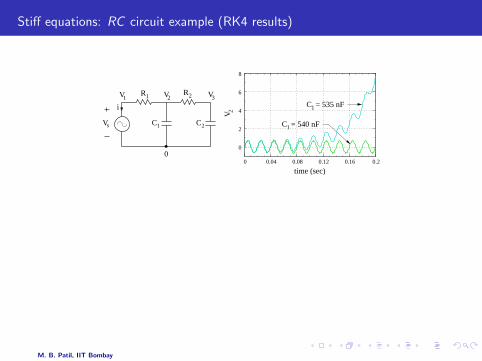
Stiff equations: RC circuit example (RK4 results)
V
C1
1R 2R
C = 535 nF1
C = 540 nF1
time (sec)
Vs
i
C2
V V V
0
2
1 2 3
0
2
4
6
8
0 0.04 0.08 0.12 0.16 0.2
* Parameters: R1 = 1 kΩ, R2 = 2 kΩ, C2 = 1 mF , f = 50 Hz, V (amplitude ofVs )=1 V , and h (step size)=1 ms.
* For f = 50 Hz, XC1 = 295 kΩ, and XC2 = 160 Ω. ⇒ C1 is effectively an opencircuit, and its exact value should have no effect on the results.
* However, for C1 = 540 nF and C1 = 535 nF , the RK4 results are dramaticallydifferent. Why?
* C1 = 535 nF makes one of the time constants in the circuit small enough (withrespect to h = 1 ms) to make the RK4 method unstable.
M. B. Patil, IIT Bombay
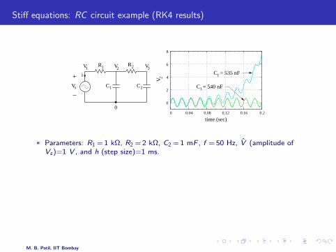
Stiff equations: RC circuit example (RK4 results)
V
C1
1R 2R
C = 535 nF1
C = 540 nF1
time (sec)
Vs
i
C2
V V V
0
2
1 2 3
0
2
4
6
8
0 0.04 0.08 0.12 0.16 0.2
* Parameters: R1 = 1 kΩ, R2 = 2 kΩ, C2 = 1 mF , f = 50 Hz, V (amplitude ofVs )=1 V , and h (step size)=1 ms.
* For f = 50 Hz, XC1 = 295 kΩ, and XC2 = 160 Ω. ⇒ C1 is effectively an opencircuit, and its exact value should have no effect on the results.
* However, for C1 = 540 nF and C1 = 535 nF , the RK4 results are dramaticallydifferent. Why?
* C1 = 535 nF makes one of the time constants in the circuit small enough (withrespect to h = 1 ms) to make the RK4 method unstable.
M. B. Patil, IIT Bombay
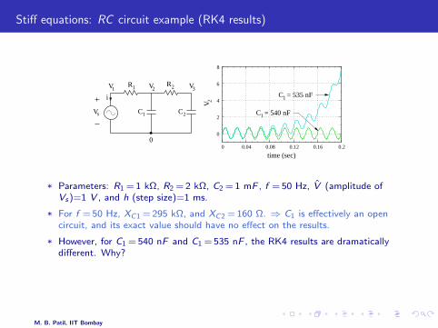
Stiff equations: RC circuit example (RK4 results)
V
C1
1R 2R
C = 535 nF1
C = 540 nF1
time (sec)
Vs
i
C2
V V V
0
2
1 2 3
0
2
4
6
8
0 0.04 0.08 0.12 0.16 0.2
* Parameters: R1 = 1 kΩ, R2 = 2 kΩ, C2 = 1 mF , f = 50 Hz, V (amplitude ofVs )=1 V , and h (step size)=1 ms.
* For f = 50 Hz, XC1 = 295 kΩ, and XC2 = 160 Ω. ⇒ C1 is effectively an opencircuit, and its exact value should have no effect on the results.
* However, for C1 = 540 nF and C1 = 535 nF , the RK4 results are dramaticallydifferent. Why?
* C1 = 535 nF makes one of the time constants in the circuit small enough (withrespect to h = 1 ms) to make the RK4 method unstable.
M. B. Patil, IIT Bombay

Outline
* Introduction and problem definition
* Taylor series methods
* Runge-Kutta methods
* Specific multi-step methods
* Generalized multi-step methods
* Predictor-corrector methods
* Numerical results
* Stability of numerical methods
* Regions of stability
* Stiff equations
* Adaptive step size
* Miscellaneous topics
M. B. Patil, IIT Bombay
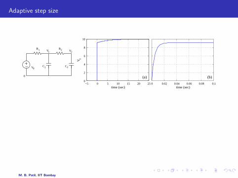
Adaptive step size
V 1
time (sec)
(a)
time (sec)
(b)
V0C C1 2
R R21
0
V1 V2
0
2
4
6
8
10
−5 0 5 10 15 20 25 0 0.02 0.04 0.06 0.08 0.1
* It is desirable to use small time steps when the solution is changing rapidly, andlarge time steps otherwise.
* For automatic time step computation, the next time step can be computed on
the basis of
- an estimate of the local truncation error (LTE)- convergence behaviour of Newton-Raphson algorithm (for nonlinear
problems)
M. B. Patil, IIT Bombay
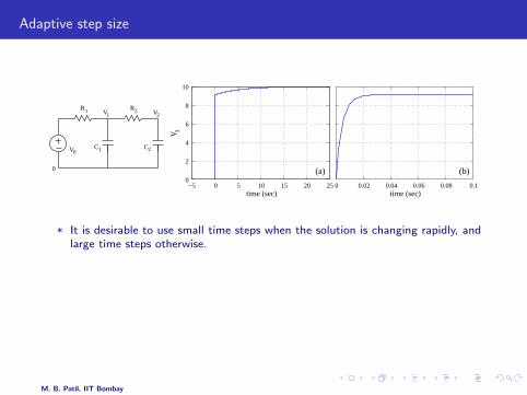
Adaptive step size
V 1
time (sec)
(a)
time (sec)
(b)
V0C C1 2
R R21
0
V1 V2
0
2
4
6
8
10
−5 0 5 10 15 20 25 0 0.02 0.04 0.06 0.08 0.1
* It is desirable to use small time steps when the solution is changing rapidly, andlarge time steps otherwise.
* For automatic time step computation, the next time step can be computed on
the basis of
- an estimate of the local truncation error (LTE)- convergence behaviour of Newton-Raphson algorithm (for nonlinear
problems)
M. B. Patil, IIT Bombay
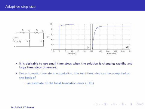
Adaptive step size
V 1
time (sec)
(a)
time (sec)
(b)
V0C C1 2
R R21
0
V1 V2
0
2
4
6
8
10
−5 0 5 10 15 20 25 0 0.02 0.04 0.06 0.08 0.1
* It is desirable to use small time steps when the solution is changing rapidly, andlarge time steps otherwise.
* For automatic time step computation, the next time step can be computed on
the basis of
- an estimate of the local truncation error (LTE)
- convergence behaviour of Newton-Raphson algorithm (for nonlinearproblems)
M. B. Patil, IIT Bombay
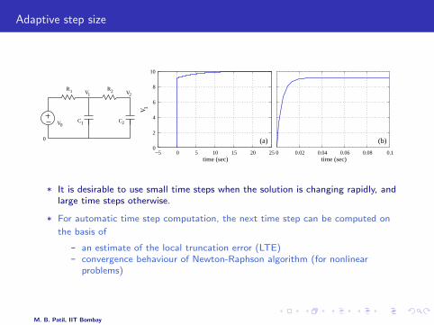
Adaptive step size
V 1
time (sec)
(a)
time (sec)
(b)
V0C C1 2
R R21
0
V1 V2
0
2
4
6
8
10
−5 0 5 10 15 20 25 0 0.02 0.04 0.06 0.08 0.1
* It is desirable to use small time steps when the solution is changing rapidly, andlarge time steps otherwise.
* For automatic time step computation, the next time step can be computed on
the basis of
- an estimate of the local truncation error (LTE)- convergence behaviour of Newton-Raphson algorithm (for nonlinear
problems)
M. B. Patil, IIT Bombay

LTE estimation: use of two time steps
* The local error of a numerical method of order p is given by,
x(tn + h)− xn+1 = hp+1ψ(tn, xn) + O(hp+2) , (29)
where ψ is called the principal error function of the method.
* If, instead of a single step of h, we take two steps of h/2 each, then the localerror would be
x(tn + h)− xn+1 = 2
(h
2
)p+1
ψ(tn, xn) + O(hp+2) , (30)
where xn+1 denotes the computed solution after the second step.
* By subtracting Eq. 29 from Eq. 30, we get an estimate for the LTE,
LTEest =
(2p
2p − 1
)|xn+1 − xn+1| . (31)
M. B. Patil, IIT Bombay
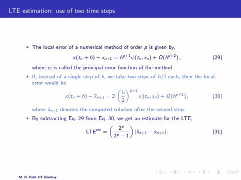
LTE estimation: use of two time steps
* The local error of a numerical method of order p is given by,
x(tn + h)− xn+1 = hp+1ψ(tn, xn) + O(hp+2) , (29)
where ψ is called the principal error function of the method.
* If, instead of a single step of h, we take two steps of h/2 each, then the localerror would be
x(tn + h)− xn+1 = 2
(h
2
)p+1
ψ(tn, xn) + O(hp+2) , (30)
where xn+1 denotes the computed solution after the second step.
* By subtracting Eq. 29 from Eq. 30, we get an estimate for the LTE,
LTEest =
(2p
2p − 1
)|xn+1 − xn+1| . (31)
M. B. Patil, IIT Bombay

LTE estimation: use of two time steps
* Suppose τ has been specified as the maximum allowed LTE.
* If LTEest < τ , the current step is accepted, and the next step is allowed toincrease (since a larger step may continue to fulfill the the constraint on theLTE).
* If LTEest > τ , the current step is rejected, and a new trial step h′n is computedsuch that it would result in an LTE equal to τ .
h′n = hn
( τ
LTEest
)1/p+1. (32)
* LTEest may also be used to improve the accuracy of the solution.
M. B. Patil, IIT Bombay

LTE estimation: use of methods of different orders
Consider two methods of orders p and (p + 1). If xn = x(tn) is assumed, we get
LTE(p) = x(tn+1)− xn+1 , (33)
LTE(p+1) = x(tn+1)− xn+1 , (34)
where the superscript on LTE indicates the order of the method, and xn+1, xn+1
denote the numerical solutions corresponding to the two methods.
Subtracting Eq. 34 from Eq. 33 yields,
LTE(p) − LTE(p+1) = xn+1 − xn+1 . (35)
Assuming that LTE(p+1) can be neglected in comparison with LTE(p) (since LTE(p+1)
is for a higher-order method), we get an estimate for LTE(p).
Note that an additional cost of computing xn+1 with a higher-order method is involvedhere. In practice, the low- and high-order methods are chosen so that some of thecomputation of the low-order method can be used for the high-order method.
M. B. Patil, IIT Bombay
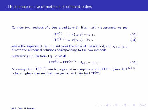
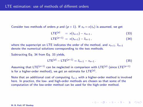
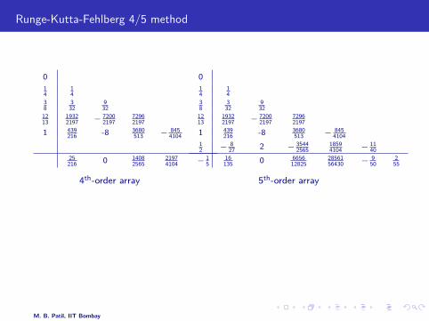
Runge-Kutta-Fehlberg 4/5 method
0
14
14
38
332
932
1213
19322197 − 7200
219772962197
1 439216 -8 3680
513 − 8454104
25216 0 1408
256521974104 − 1
5
4th-order array
0
14
14
38
332
932
1213
19322197 − 7200
219772962197
1 439216 -8 3680
513 − 8454104
12 − 8
27 2 − 35442565
18594104 − 11
40
16135 0 6656
128252856156430 − 9
502
55
5th-order array
* Since the function values, f0, f1, · · · , f4 are the same in the two methods, only sixfunction evaluations are required in each time step.
* The estimated LTE of the fourth-order formula is given by,
LTEest = h
[1
360f0 −
128
4275f2 −
2197
25740f3 +
1
50f4 +
2
55f5
]. (36)
M. B. Patil, IIT Bombay
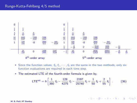
Runge-Kutta-Fehlberg 4/5 method
0
14
14
38
332
932
1213
19322197 − 7200
219772962197
1 439216 -8 3680
513 − 8454104
25216 0 1408
256521974104 − 1
5
4th-order array
0
14
14
38
332
932
1213
19322197 − 7200
219772962197
1 439216 -8 3680
513 − 8454104
12 − 8
27 2 − 35442565
18594104 − 11
40
16135 0 6656
128252856156430 − 9
502
55
5th-order array
* Since the function values, f0, f1, · · · , f4 are the same in the two methods, only sixfunction evaluations are required in each time step.
* The estimated LTE of the fourth-order formula is given by,
LTEest = h
[1
360f0 −
128
4275f2 −
2197
25740f3 +
1
50f4 +
2
55f5
]. (36)
M. B. Patil, IIT Bombay
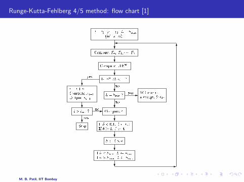
Runge-Kutta-Fehlberg 4/5 method: flow chart [1]
t = t0; x = x0; h = hmax(initialize)Compute LTEest
t = t+ hCompute xn+1Output xn+1 h = hmin ? Write errormessage. Stop.
If h > hmax; h hmaxIf h < hmin; h hminStop If Æ < 0:1; Æ 0:1If Æ > 4; Æ 4
Compute F0; F1; ; F5LTEest=h < ?
t > tend ? Compute Æyes no yesnoyes no
h Æ hM. B. Patil, IIT Bombay

Runge-Kutta-Fehlberg 4/5 method: example
1V
V2
RV1
12 Vs
0
V2
C
h (m
sec)
−1
0
1
2
3
4
5
6
0 5 10 15
V ,
V (
Vol
ts)
time (msec)
0
0.4
0.8
1.2
0 5 10 15time (msec)
* Parameters: R = 1 kΩ, C = 1 µF , hmin = 1 ns, hmax = 1 ms,ε (tolerance)=10 mV .
* When the solution is changing rapidly, the time step is made small in order tomeet the tolerance requirement.
* When the solution is changing slowly, the time step is made large (capped by auser-specified hmax).
M. B. Patil, IIT Bombay
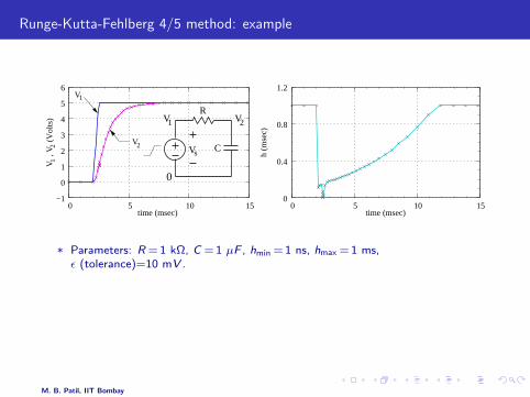
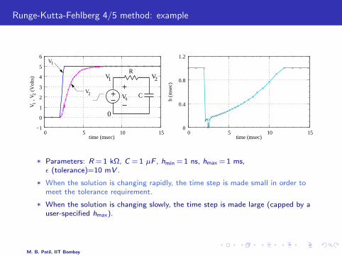
Adaptive step size: convergence of N-R iterations
* The Newton-Raphson process is more likely to converge (in a given number ofiterations) if the starting point, i.e., the “initial guess”, is close to the solution.
* In transient analysis, xn serves as the starting point, and xn+1 is the solutionbeing sought.
* If the time step, (tn+1 − tn), is made smaller, the initial guess xn is expected tobe closer to the solution xn+1, and the N-R process is more likely to converge.
* The above observation is commonly used in circuit simulation for controlling thetime step. (It works only for non-linear problems.)
M. B. Patil, IIT Bombay
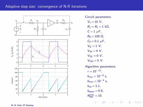
Adaptive step size: convergence of N-R iterations
V2
V4
42
µ
V1
Vs
V2
R2
0
C
R1 R
C
0
0
VV4
3
0
1
2
3
4
5
2 3 4 5 6
V ,
V (
Vol
ts)
0
20
40
60
80
100
120
2 3 4 5 6time (msec)
h (
sec
)
Circuit parameters:
Vs = 10 V ,
R1 = R2 = 1 kΩ,
C = 1 µF ,
R0 = 100 Ω,
C0 = 0.1 µF ,
VIL = 1 V ,
VIH = 4 V ,
VOL = 0 V ,
VOH = 5 V .
Algorithm parameters:
τ = 10−12,
hmin = 10−9 s,
hmax = 10−4 s,
kup = 1.1,
kdown = 0.8,
NmaxNR = 10.
M. B. Patil, IIT Bombay

Transient analysis in circuit simulation
* The method must be zero-stable (i.e., stable for small h).
* There are small time constants involved in many circuits. Methods which areconditionally stable are not practical since they will require unacceptably smalltime steps. ⇒ The method must be A-stable.
* The above considerations severely restrict the choice of methods available: OnlyAM1 (BE), AM2 (TRZ), BDF2, and implicit Runge-Kutta methods may beused.
* Application of the MNA method to circuits would generally yield a set ofequations of the following type [7]:
F(x′, x, y, t) = 0 , (37)
G(x, y, t) = 0 . (38)
Equations in the above form are called “Differential-algebraic equations(DAEs).”
* Runge-Kutta methods are not suitable for DAEs. ⇒ The choice is furtherreduced to BE, TRZ, BDF2.
M. B. Patil, IIT Bombay

Outline
* Introduction and problem definition
* Taylor series methods
* Runge-Kutta methods
* Specific multi-step methods
* Generalized multi-step methods
* Predictor-corrector methods
* Numerical results
* Stability of numerical methods
* Regions of stability
* Stiff equations
* Adaptive step size
* Miscellaneous topics
M. B. Patil, IIT Bombay
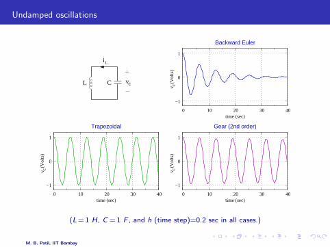
Undamped oscillations
CL v
i
c
c c
c
L
v (
Vol
ts)
v (
Vol
ts)
v (
Vol
ts)
−1
0
1
0 10 20 30 40time (sec)
−1
0
1
0 10 20 30 40time (sec)
−1
0
1
0 10 20 30 40time (sec)
Trapezoidal
Backward Euler
Gear (2nd order)
(L = 1 H, C = 1 F , and h (time step)=0.2 sec in all cases.)
M. B. Patil, IIT Bombay
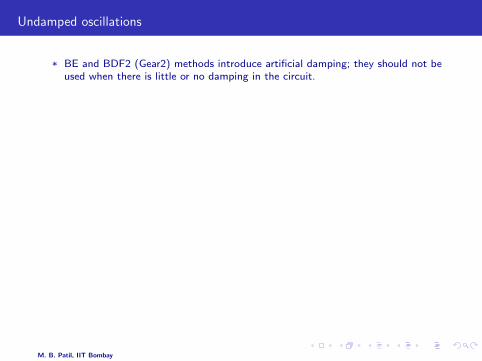
Undamped oscillations
* BE and BDF2 (Gear2) methods introduce artificial damping; they should not beused when there is little or no damping in the circuit.
* TRZ method does not introduce artificial damping.
* However, even the TRZ method is not perfect for purely oscillator problemssince it does introduce some phase error. ⇒ need to select a small time step.
TRZExact
c
−1
−0.5
0
0.5
1
40 50 60 70 80time (sec)
v (
Vol
ts)
M. B. Patil, IIT Bombay
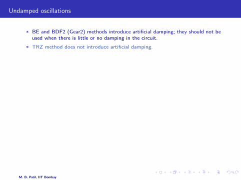
Undamped oscillations
* BE and BDF2 (Gear2) methods introduce artificial damping; they should not beused when there is little or no damping in the circuit.
* TRZ method does not introduce artificial damping.
* However, even the TRZ method is not perfect for purely oscillator problemssince it does introduce some phase error. ⇒ need to select a small time step.
TRZExact
c
−1
−0.5
0
0.5
1
40 50 60 70 80time (sec)
v (
Vol
ts)
M. B. Patil, IIT Bombay
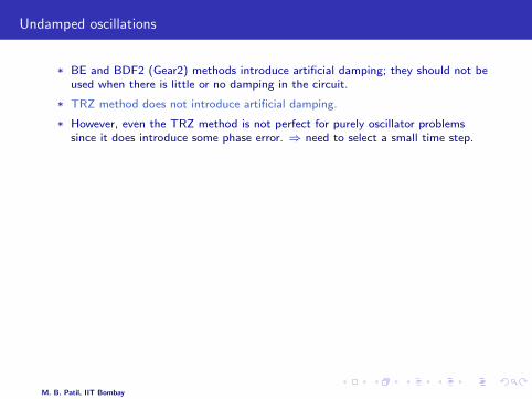
Undamped oscillations
* BE and BDF2 (Gear2) methods introduce artificial damping; they should not beused when there is little or no damping in the circuit.
* TRZ method does not introduce artificial damping.
* However, even the TRZ method is not perfect for purely oscillator problemssince it does introduce some phase error. ⇒ need to select a small time step.
TRZExact
c
−1
−0.5
0
0.5
1
40 50 60 70 80time (sec)
v (
Vol
ts)
M. B. Patil, IIT Bombay
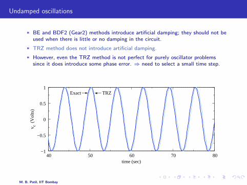
Undamped oscillations
* BE and BDF2 (Gear2) methods introduce artificial damping; they should not beused when there is little or no damping in the circuit.
* TRZ method does not introduce artificial damping.
* However, even the TRZ method is not perfect for purely oscillator problemssince it does introduce some phase error. ⇒ need to select a small time step.
TRZExact
c
−1
−0.5
0
0.5
1
40 50 60 70 80time (sec)
v (
Vol
ts)
M. B. Patil, IIT Bombay

Ringing
Vs
V1V2
R
(b)
(c)
1
(a)
C
0
−10
0
10
20
30expected
BE
−10
0
10
20
30
0 50 100
expectedTRZ
curr
ent (
mA
)cu
rren
t (m
A)
time (msec)time (msec) 0 50 100
0
0.2
0.4
0.6
0.8
1
1.2
V (
Vol
ts)
(Parameters: R = 1 Ω, C = 1 mF , and h (time step) = 5 msec.)
* If h is large, TRZ results in ringing.
* Ringing can be reduced by using a smaller time step.
M. B. Patil, IIT Bombay
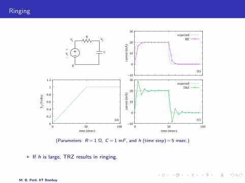
Ringing
Vs
V1V2
R
(b)
(c)
1
(a)
C
0
−10
0
10
20
30expected
BE
−10
0
10
20
30
0 50 100
expectedTRZ
curr
ent (
mA
)cu
rren
t (m
A)
time (msec)time (msec) 0 50 100
0
0.2
0.4
0.6
0.8
1
1.2
V (
Vol
ts)
(Parameters: R = 1 Ω, C = 1 mF , and h (time step) = 5 msec.)
* If h is large, TRZ results in ringing.
* Ringing can be reduced by using a smaller time step.
M. B. Patil, IIT Bombay

References
[1] R. L. Burden and J. D. Faires, Numerical Analysis, Singapore: Thomson, 2001.
[2] M. B. Patil, V. Ramanarayanan, and V. T. Ranganathan, Simulation of Power ElectronicCircuits, to be published.
[3] C. F. Gerald and P. O. Whitley, Applied Numerical Analysis, Delhi: Pearson Education India,1999.
[4] L. Lapidus and J. H. Seinfeld, Numerical solution of ordinary differential, New York:Academic Press, 1971.
[5] L. F. Shampine, Numerical solution of ordinary differential equations, New York: Chapmanand Hall, 1994.
[6] L. O. Chua and P. M. Lin, Computer-Aided Analysis of Electronic Circuits, Englewood Cliffs:Prentice-Hall, 1976.
[7] K. E. Brenan, S. L. Campbell, and L. R. Petzold, Numerical Solution of Initial-ValueProblems in Differential-Algebraic Equations, New York: North-Holland, 1989.
M. B. Patil, IIT Bombay