chemistry of vibronic coupling, part 4: off-diagonal vibronic
TRANSCRIPT

Chemistry of Vibronic Coupling, Part 4: Off-DiagonalVibronic Coupling Constants Across the Periodic Table
by W. Grochala and R. Hoffmann*
Department of Chemistry and Chemical Biology, Cornell University, Ithaca NY, 14853-1301 USA
(Received April 27th, 2001)
Vibronic coupling for inter–valence charge–transfer states in linear symmetric ABAmolecules (A, B = s–, p– or d–block element) is investigated computationally. In particu-lar we examine vibronic coupling as a function of the s, p, d – block nature of the A and Bconstituent elements. Based on density-functional theory computations for 395 triatomicmolecules, we construct a map of a vibronic stability parameter G (defined as the ratio ofasymmetric to symmetric stretching force constants) across the periodic table. Correla-tions of G versus the sum and difference of electronegativities of A and B elements aretested, and also vs. a useful parameter f, the ratio of the sum of electronegativities to anAB separation. Usually, the larger the sum of electronegativities, and the shorter the ABbond, the larger the vibronic instability. The largest vibronic instability thus occurs forinterhalogen compounds. Molecules containing d-block elements exhibit trends similarto those of molecules built of p-block elements with similar electronegativities, althoughthe latter are usually more unstable.A molecular orbital model is developed to explain the trends obtained in our computa-tions, as well as to build a framework for systematic manipulation of vibronic couplingconstants in molecular systems. From the model we argue that vibronic coupling is usu-ally strongest in systems built of hard Lewis acids and bases. We also show that s–p mix-ing and “ionic/covalent curve crossing” increase the vibronic instability of a molecule.To attain high vibronic instability, one should build a molecule of light, highly electro-negative p–block elements. These findings may be of use in the experimental search fornew superconducting materials.
Key words: triatomic radicals, quantum mechanical calculations, vibronic coupling,hardness, avoided crossing
There are many theories of solid-state superconductivity (SC), the best known be-ing the BCS theory [1]. The electron-phonon coupling constant (EPCC) and the den-sity of states at the Fermi level (DOSF) are the most important parameters in the BCStheory. The theory predicts that the critical superconducting temperature (Tc) is highwhen both DOSF and EPCC are large. Although the BCS theory cannot quantitativelyexplain high-temperature superconductivity, there is strong evidence of the impor-tance of vibronic effects for the latter as well [2]. This is where our interest in vibronic
Polish J. Chem., 75, 1603–1659 (2001)
*Author to whom correspondence should be addressed, e-mail:[email protected]

coupling constants (VCCs, the molecular analogue of the EPCCs), detailed in severalpreceding papers, originates. We investigate simple AB and A2B
� molecular systems,aiming to find the relationships between the chemical nature of the elements consti-tuting these systems and their propensity to vibronic instability. Our eventual goal isto develop a chemical strategy for tuning VCCs and EPCCs.
In our first paper we studied the behavior of VCC� egi [eV] within a broad space of
three parameters: force constant (k), displacement along symmetry-breaking normalcoordinate (�Q) and reduced oscillator mass (m) [3].
� egi = (� eg
i )v = h egi x <ug|Qi|ve> [eV] (1a) h eg
i (Qi) = <g|�H/�Qi|e> [eV/Å] (1b)
where g and e are the diabatic electronic wavefunctions of two vibronically coupledelectronic states, ug and ve are vibrational wavefunctions for normal mode i, in g and estates respectively, and �H/�Qi is the derivative of Hamiltonian along the normal co-ordinate Qi through which coupling occurs.
We concluded that maximizing� egi requires precise control of the nuclear geome-
try appropriate for a given (k, m) pair. Subsequently we concentrated on diagonal andoff-diagonal linear dynamic VCCs. In a second paper we investigated the diagonalVCC (h ee
i ) for T1 states of AB molecules where A, B = alkali metal, H or halide [4]. Aparameter f, defined as a sum of Pauling electronegativities of the A and B elementsdivided by AB bond length:
f = fAB = (ENA + ENB)/ RAB (2)
was found to be very useful in correlating h eei for three distinct classes of molecules:
intermetallics (M1M2), interhalogens (X1X2) and “salts” (MX), including metal hy-drides (MH) and hydrogen halides (HX).
Subsequently we looked at the off-diagonal VCC (h egi ) for triatomic linear ABA
molecules where A, B = alkali metal, H or halide [5]. We found that the same parame-ter f is of value in a qualitative description of h eg
i : large values of f usually indicatelarge h eg
i . We noted the utility of f for qualitative studies of vibronic coupling in threefamilies of ABA molecules: intermetallic species M2M�, interhalogen species X2X�and “salts” (M2X and X2M).
This paper is the fourth part in the series “Chemistry of Vibronic Coupling”. Wenow broaden the range of molecules for which VCC’s are studied [6]: we study h eg
i forABA� molecules where A, B = s, p, d block element. We try to see which type of or-bital (s, p, or d) helps to maximize off-diagonal VCC’s in A2B
� systems. We alsoexplain the trends observed using a molecular orbital (MO) model.
In our next pape [7] we will try to show how the considerations of vibronic cou-pling constants for simple molecules may be extended to solid state systems withhigh-symmetry lattices.
1604 W. Grochala and R. Hoffmann

METHODS OF CALCULATIONS
A description of the vibronic coupling model used here may be found in the Methods of Calculations
section of [3]. Numerical data (shown in Supplement, Tables S1 and S2) have been obtained from densityfunctional theory (DFT) B3LYP computations with a 6-311++G** basis set for light elements andLANL2DZ core potentials for heavier s- and p-block elements (for details see [4]) and for all d-block ele-ments. An equilibrium AB bond length has been computed while constraining the ABA species to be lin-ear. Force constants for the symmetric and antisymmetric stretching modes have been subsequentlycomputed.
We have used the following computational packages: Gaussian’94 [8] and HyperChem 5.0 [9] forSCF and DFT calculations, YAEHMOP [10] and CACAO [11] for EH calculations.
Tables S1 and S2 may be found in the Supplementary Material to this paper.
RESULTS AND DISCUSSION
1. DFT Computations of the Off-Diagonal Vibronic Coupling Constant.
1.1. hegi for Inter Valence Charge Transfer States of ABA Molecules where
A, B = s, p – block Element.
In this section we concentrate on linear triatomic radicals of the general formulaABA�. Such molecules are ideal for studying the off-diagonal VCC h eg
i for theantisymmetric stretching mode. This parameter is often studied with relevance to sys-tems exhibiting a second order Jahn-Teller effect [12]. Previously we had investi-gated 100 linear symmetric ABA� molecules [13] for A, B = H, alkali metal or halide[5]. Now we broaden this study to all s– and p–blocks of elements, investigating anadditional 240 ABA� molecules [14]. Numerical data for all 340 molecules are shownin Table S1 in the Supplement.
Our focus in this study is on a parameter G. We introduced G while studyingvibronic coupling for ABA� radicals where A, B = alkali metal, halide or H [5]; G isdefined as ratio of force constants for the asymmetric and symmetric stretchingmode:
G = ku/kg (3)
This dimensionless parameter is very useful as a quantitative description of the“asymmetric mode softening” which follows from vibronic coupling. Large positivevalues of G imply vibronic stability of a linear molecule along the asymmetricstretching coordinate (Qas). Small positive values of G correspond to asymmetricmode softening, i.e. substantial vibronic coupling along Qas. Negative G impliesstrong vibronic coupling and instability of the molecule along Qas.
The electronegativity, as problematic as its definition is [15], is an obvious“chemical” parameter with which one might correlate G. Since the 1930’s electro-negativity differences have been identified with bond polarity [16], and subsequentlyused in diverse chemical problems (heats of formation [17], X-ray absorption edgeshifts [18], XPES [19], IR [20]). Occasionally, a difference of ionization potentialshas also been used [21]. On the other hand, the sum of electronegativities (which we
Chemistry of vibronic coupling... 1605

will use later in the paper) has been successfully applied to describe qualitativelybonding between chemical elements in solid state in the Arkel-Ketlaar diagrams [22],and to evaluate the total inductive effect of the substituents on a carbon or tin atom[23]. Parr and Pearson, using density functional theory, first introduced hardness, aparameter closely related to electronegativity [24]. Differences of hardnesses havebeen successfully used to derive bond energies [25], and to classify binary octet com-pounds [26]. On the other hand, the sum of hardnesses has been applied to constructphase diagrams in solid state [27]. Our contribution is the recognition of the utility ofthe parameter f (the sum of electronegativities divided by distance) for quantitativecorrelations [28]. As far as we know, a similar approach has been used only once incorrelation between the experimental values of force constants and forces in diatomicH-containing molecules [29].
Why ABA radicals? The reason is that the asymmetrization process in such linearspecies contains the essential electron transport component that characterizes con-ductivity: A+–B– + A0 � A–B–A � A0 + B––A+.
We discuss in this paper the motion of symmetric linear ABA molecules exclu-sively along an asymmetric stretching coordinate. Why do we constrain ABA mole-cules to a linear geometry, which may not necessarily correspond to the ground stateof a molecule? The reason for that is that in the linear geometry there is a particularlyeffective and simple way to analyze coupling of the antisymmetric stretching modewith the charge-transfer process between A centers.
We need to emphasize here that, as important as some of these molecules are intheir own right, we are interested neither in computing the lowest energy geometry fora given system [30], nor in providing a description of the whole potential energy sur-face determining dynamics of, for instance, the “SN2” A–B–A � A0 + B––A+ reaction[31]. Both tasks would require geometry optimization of a triatomic in a full space ofnuclear coordinates. Our goal is something different, namely a comparison ofvibronic stabilities within a certain class of species (linear symmetric radicals [32]),in the search for chemical trends and useful correlations.
In seeking such trends and correlations, we plot G versus the difference ofPauling electronegativities of B and A elements (� EN) constituting ABA� molecule.Two kinds of such plots will be of particular importance: one emphasizes the affilia-tion of B to a given group of the periodic table, another to a given period. In Figs. 1 and2 we show such plots (for periods II and V). In Figs. 3 and 4 we plot G versus �EN (forgroups 1 and 13). To highlight the regularities, in each case some lines are sketchedwhich connect in a schematic way (these are not fits) the points for a given element.
It appears that there are three kinds of shapes of G vs �EN plot, dependingwhether B is a typical nonmetal or a typical metal, or is intermediate between the two.
i) For B a typical nonmetal, such as F or O, the plot seems to peak at a certain � EN(we will call it hereafter � ENpeak). G decreases steeply from � ENpeak towardmore negative and more positive values of � EN. The formal borderline of � EN= 0 (for � EN < 0, B serves as the anion in an A2B
� molecule, for � EN > 0, Bserves as the cation) appears to play no important role for G. The position of the
1606 W. Grochala and R. Hoffmann

Chemistry of vibronic coupling... 1607
Figure 1. G for triatomic A2B linear symmetric molecules, plotted vs difference of Pauling electro-negativities of B and A elements; � EN = ENB – ENA. A belongs to IInd period (data for H arealso shown). Schematic lines for A= fluorine, boron, lithium (not a fit in any way) have beenintroduced to guide the eye.

1608 W. Grochala and R. Hoffmann
Figure 2. G for triatomic A2B linear symmetric molecules, plotted vs difference of Pauling electro-negativities of B and A elements; � EN = ENB – ENA. A belongs to Vth period of the periodictable. Schematic lines for A= rubidium, iodine have been introduced to guide the eye.

Chemistry of vibronic coupling... 1609
Figure 3. G for triatomic A2B linear symmetric molecules, plotted vs difference of Pauling electro-negativities of B and A elements; � EN = ENB – ENA. A belongs to Ist main group of the peri-odic table. Schematic lines for two branches of points for A= sodium have been introduced as aguide.

1610 W. Grochala and R. Hoffmann
Figure 4. G for triatomic A2B linear symmetric molecules, plotted vs difference of Pauling electro-negativities of B and A elements; � EN = ENB – ENA. A belongs to IIIrd main group of the peri-odic table. Schematic lines for A= thallium, boron have been introduced as a guide.

� ENpeak usually occurs for � EN < 0, but is characteristic for a particular ele-ment B.
ii) The second type of plot is for B a typical metal such as Li or K. Its shape is com-plicated. It is composed of two branches of points: one for intermetallic A2Bmolecules (near � EN = 0) and another one for “salts” (at large positive valuesof � EN). G usually increases as a function of � EN within the second branch. Itseems difficult to define a transition between the two branches.
iii) The third type of plot is found for B a semimetal (such as Sb) or a poor metal(such as Tl). It is characterized by a less steep decrease of G vs � EN depend-ence than for nonmetals. The shape of the G vs � EN plot seems to be intermedi-ate between the metal- and nonmetal-type plots. It is exemplified by the rightpart of the plot for I, and by the left part for Rb (Fig. 2). As may be seen from Fig. 4,the transition between a metal- to semimetal- and nonmetal-type dependence issmooth, as exemplified by triatomics containing group IIIA elements.
We have observed similar features studying plots (not presented here) for ele-ments from all other groups and periods of periodic table.
In an attempt to visualize better the dependence of the vibronic stability parame-ter G on the chemical nature of A and B elements, we construct a map of G within theperiodic table. This is a complicated map, so in Fig. 5 we show first a “guide” to thismap; it is useful in defining some of the regions. The ordinate is the difference ofPauling electronegativities of A and B elements constituting the A2B molecule (�EN). The abscissa is the sum of Pauling electronegativities of B and A elements (ENA
+ ENB). “Ionic” molecules may be found at left and right of the diagram. “Covalent”molecules are found in the middle of the diagram. Cs3, F3, Cs2F and CsF2 moleculesdetermine the corners of the diagram. The plot is divided roughly into four areas:“intermetallic” (s,s,s) molecules, “salt-like” (s,p,s) and (p,s,p) molecules and (p,p,p)molecules built of nonmetals. The black dot represents a homonuclear A3 molecule.Orange solid lines indicate the position of possible A2B and AB2 molecules where Aformally serves as anion. A2B and AB2 molecules, where A formally serves as cation,are found along the orange dotted lines. The labels “ionic” and “covalent” refer not tomolecules in a given square, but to a rough region where |� EN| is large and small, re-spectively.
G behaves in a very interesting way, as Fig. 6, the actual map, shows. Salt-like andintermetallic molecules are vibronically stable (G � 2). Molecules built of nonmetalsare vibronically unstable (G < 0). There is a formal borderline between vibronic sta-bility and instability (the isoline G = 0). The isoline for G = 1 (indication of substan-tial asymmetric mode softening) is readily visible in Fig. 6. The transition between G
= 1 and G = 0 regions is relatively steep, indicating that tuning of G might be a prob-lem in practice.
A slight left-right asymmetry of the map presented in Fig. 6 is its interesting fea-ture. The vibronic stability of ABA and BAB molecules is, of course, not the same.This is especially clear for molecules containing nonmetals (upper part of map in Fig. 6).Typically, the instability of BAB molecules, where B is the more electronegative ele-
Chemistry of vibronic coupling... 1611

1612 W. Grochala and R. Hoffmann
Figure 5. Schematic guide-plot for Fig.3. The ordinate is the difference of Pauling electronegativities ofA and B elements constituting the A2B molecule (� EN). The abscissa is the sum of Paulingelectronegativities of B and A elements (ENA + ENB). “Ionic” molecules may be found at leftand right of the diagram. “Covalent” molecules are found in the middle of the diagram. The la-bels “ionic” and “covalent” refer not to molecules in a given square, but to a rough region where|� EN| is large and small, respectively. Cs3, F3, Cs2F and CsF2 molecules determine the cornersof the diagram. The plot is divided roughly into four areas: “intermetallic” (s,s,s) molecules,“salt-like” (s,p,s) and (p,s,p) molecules and (p,p,p) molecules built of nonmetals. The black dotrepresents a homonuclear A3 molecule. Orange solid lines indicate the position of possible A2Band AB2 molecules, where A formally serves as anion. A2B and AB2 molecules, where A for-mally serves as cation, are found along the orange dotted lines.

Chemistry of vibronic coupling... 1613
Figure 6. Map of vibronic stability parameter (G) in the periodic table of elements. The ordinate is � EN,the abscissa is (ENA + ENB). For a more detailed description see text. Fig. 5 is a guide to thisplot.
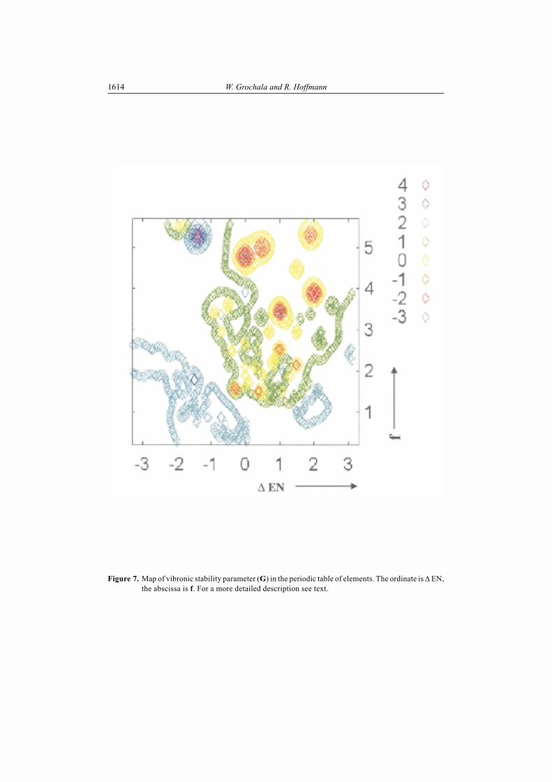
1614 W. Grochala and R. Hoffmann
Figure 7. Map of vibronic stability parameter (G) in the periodic table of elements. The ordinate is � EN,the abscissa is f. For a more detailed description see text.

ment, (such as F2H with G = –0.31) is smaller than that of ABA molecules (such asH2F with G = –1.33) [33].
Previously we found that parameter f (see Eq. 2 above, f is the sum of theelectronegativities divided by the equilibrium bond length) is of use in describingvibronic effects in AB and A2B molecules [4,5]. Let us try then to correlate G with f (fsubstitutes (ENA + ENB) as a variable in Fig. 6). This new map is presented in Fig. 7.
Fig. 7 resembles Fig. 6 in its general shape. Molecules with large values of f arethe most vibronically unstable species. The left-right asymmetry of the plot presentedin Fig. 7 is even more evident than in Fig. 6. It is remarkable that this simple empiricalparameter, f, again proves useful for a qualitative description of the vibronic couplingphenomenon.
The primary conclusions of this section are:i) In looking for large vibronic instability in A2B molecules one should search
among molecules with large f [34]. Such species are usually built of nonmetalswith short AB bonds.
ii) ABA molecules (where B is more electronegative than A) are usually morevibronically unstable than the corresponding BAB molecules.
Let us now examine vibronic coupling in triatomic linear symmetric moleculescontaining d-block elements as well.
1.2. hegi for IVCT States of ABA Molecules where A = s, p – block Element, B = d –
block Element.
The p- (C [35], Bi [36]) and especially the d-block elements (Cu [37], recently Hf[38]) are at the heart of real breakthroughs in solid-state superconductivity. We willnow examine vibronic coupling in molecules containing d-block elements.
Studying molecules containing d-block elements requires assuming a certainmultiplicity. For consistency, and to compare molecules containing s-, p- and d-blockelements, we will limit our mixed-valence A2B
� radicals to doublet states. Such statesmay or may not be the ground state of the molecule in question.
We have investigated molecules containing two distinct sets of d-block metals.One group contains Ti, Zr and Hf – the most electropositive elements in the d-block(ENHf = 1.3, compare to ENMg = 1.2). Another set contains noble and semi-noble met-als (group VIIIB and IXB) – the most electronegative elements in the d-block (ENAu =2.5, compare to ENI = 2.5). Molecules containing d-block elements would occupy abroad space in our Fig. 5.
Is there a bridge between vibronic coupling in molecules containing s- andp-block elements and those with d-block elements? May such a connection be de-scribed using such simple empirical parameters as EN or f? How might one distin-guish between Cu, Hg, Bi, Fe, Re, whose electronegativity is nearly equal? We do not
expect that electronegativity – although useful in so many areas of chemistry – willdescribe well the whole richness of so many features of different elements. Let us,however, make a try. If we used the map presented in Fig. 6 as a guide for molecules
Chemistry of vibronic coupling... 1615

containing d-block elements, we would conclude that most such A2B moleculesshould be vibronically unstable (especially these containing noble metals). Some ofthese molecules might be subject only to significant asymmetric mode softening.
Let us now confront these expectations with the result of DFT computations. Fig. 8plots the vibronic stability parameter G for chosen linear symmetric A2B molecules[39] vs. the difference of Pauling electronegativities of A and B elements (A is a givend-block element, B is a s- or p-block element).
It is clear from Fig.8 that triatomics containing d-block elements do not behave aspredicted based on trends for s- and p-block elements. All the molecules investigatedare vibronically stable, contrary to our expectations [40]. There is substantial vibro-nic coupling (G < 1.5) in seven molecules: four Au-containing ones, one Ru-contai-ning one, and two Os-containing ones. Absolute values of G for triatomics containingd-block elements are, however, larger than for the respective p-block elements con-taining molecules of similar EN.
Are not there any similarities in vibronic stability in p-block- and d-block-containing molecules? We think there are. The shape of G vs. � EN dependence forAu is very similar to that observed before for I (iodine) – it is typical of nonmetals orpoor metals. On other hand, the general shape of the G vs. � EN dependence for Cu ismore similar to that observed before for metallic s- and p-block elements. This docu-ments that vibronic stability in molecules containing d-block elements exhibitstrends similar to ones observed for molecules containing s- and p-block elements.
2. Model of Vibronic Coupling Along Qas in Symmetric Linear ABA� systems – MO
Picture.
How to understand and predict in a qualitative way vibronic stability or instabilityin a large family of linear symmetric triatomics? We will try to answer this questionusing first a simple molecular orbital model. Two levels of theory are explored: ex-tended Hückel theory (EH) and DFT. EH will help us establish a framework of discus-sion for vibronic effects. DFT will enable us to add more subtle quantitative effects tothe qualitative backbone introduced by EH.
2.1. Vibronic Coupling in the Extended Hückel Model.
Simplistic thinking within EH helped us build a qualitative framework forvibronic coupling [41]. Let us use now a similar approach. We choose a linear sym-metric H3 molecule as a general model for A3 molecules. Let us follow the normal co-ordinate for antisymmetric stretching (Q = Qas) in this system and observe whathappens to the MOs.
Fig. 9 shows the molecular orbitals for H3 molecule during distortion along Qas.The starting geometry has an H–H bond length of 0.931 Å (the result of a DFT optimi-zation for a linear H3 constrained to be symmetric). Schematic drawings illustrate thecontribution of the atomic orbitals to the MOs of H3.
1616 W. Grochala and R. Hoffmann

Chemistry of vibronic coupling... 1617
Figure 8a. Plot of vibronic stability parameter G for linear symmetric A2B molecules vs. difference ofPauling electronegativities of B and A elements. a) A belongs to group 10 or 4. B = alkalimetal, H or halogen. Arbitrarily drawn lines have been introduced to guide the eye to trendsfor A= Cu, Au.

1618 W. Grochala and R. Hoffmann
Figure 8b. Plot of vibronic stability parameter G for linear symmetric A2B molecules vs. difference ofPauling electronegativities of B and A elements. b) A belongs to “noble metals”. B = alkalimetal, H or halogen.

The evolution of the MOs of H3 during distortion is easily described. There arethree � MOs. In order of increasing energy these are the �g (SOMO-1), �u (SOMO)and � g
* (SOMO+1) of the undistorted i.e. symmetric molecule (SOMO is a singly oc-cupied molecular orbital). The �g is nearest neighbor H–H bonding, �u is nonbondingand� g
* is antibonding. In Dh these canonical orbitals do not mix. However, as the Dh
symmetry is broken in a deformation along Qas, all � orbitals may mix with one an-other. There is a decrease in energy connected with this distortion (for 3 electrons inthe system). In the discussion that follows we use the �g, �u and � g
* notation for thethree MO’s even when the symmetry is lowered to Cv along Qas.
Chemistry of vibronic coupling... 1619
Figure 9. Following the normal coordinate for an antisymmetric stretch Qas in a linear symmetric H3
molecule (the EH computation). The sizes of the circles are a schematic indication of the AOcontribution in the MO; the actual percentages are given.

The orbitals of a significantly asymmetric molecule are substantially different.For (exaggerated) Qas = 0.45 Å the SOMO and SOMO + 1 resemble bonding andantibonding � and �* orbitals of an H2 molecule and the SOMO has its main contribu-tion from an “isolated” H atom. The result is expected; an excursion along Qas bringsabout localization to a single strongly bound H–H molecule and an H atom.
Let us trace the perturbation of this MO scheme as we change the extendedHückel Coulomb parameter Hii for the middle H atom. In this way we can simulate thesubstitution of the central atom by more electronegative/electropositive elements,which is what the G or ku plots study. We have varied the Hückel Hii for the middle Hatom over broad limits (keeping the H–H separation of R0 = 0.931 Å = const., as opti-mized for a symmetric linear H3 molecule at the B3LYP/6-311++G** level).
The resulting energy levels and schematic MO pictures are presented in Fig. 10.We show three extreme cases: the difference of Hückel parameters between cen-
tral and side H atoms (� Hii defined as Hii (H�) – Hii (H) in an HH�H molecule; � Hii isused as a variable in Figs. 12, 13 and 14) being a) –15 eV, b) 0 eV and c) +15 eV. Thestarting point is the standard hydrogen Hii of –13.6 eV. The Hii’s of the terminal atomsare kept constant, only that of the central atom is varied. Cases a) and c) simulate (inexaggerated manner) the electronegativity effect of substitution in H2F and H2Csmolecules, respectively [42]. We will therefore denote these cases as H2X and H2M,respectively.
What are the basic similarities and differences between the three cases presentedin Fig. 10? First, we immediately notice no change in the shape and energy of theSOMO (�u). This is obvious, considering that the perturbation is in the nodal plane ofthe �u. In a self-consistent calculation, the energy of the �u will actually change as theelectronegativity of the perturbed ligands makes the end atoms more or less positive.Second, the � Hii = –15 eV and � Hii = +15 eV cases are rough “mirror images” of eachother. We mean here that contributions from atomic orbitals to �g for � Hii = –15 eVare close to contributions from the same atomic orbitals to � g
* for � Hii = +15 eV (ex-cept for the different H-H bonding/antibonding character of both MOs). The same istrue for � g
* at � Hii = –15 eV and �g at � Hii = +15 eV. Third, and as expected, pairedorbitals (SOMO±1, i.e. �g and � g
* ) localize, so that in the bonding MO the density islarger on the more electronegative atom, while the reverse is true in the antibondingMO [43]. As a consequence of that localization the charge distribution in “H2X” and“H2M” is, respectively, closer to (H2
+�)X– and (H2�)M+, rather than H2(X
�) andH2(M
�). Fourth, as may be seen in Fig. 6b, the energy of �g strongly increases in direc-tion H2X � H3 � H2M while the energy of � g
* strongly decreases in the same direc-tion.
Let us take now a vibronic coupling perspective on the three cases analyzed.Using perturbation theory, one may write the expression for the perturbed wave-function of a given i-th MO as:
1620 W. Grochala and R. Hoffmann

� � �i i
ij
i j
j
i j
H
E E
' 0� �
�'
0 0
0 (4)
where� i' is the perturbed wavefunction of the i-th MO, � i
0 is the initial wavefunctionof the i-th MO, � j
0 is the initial wavefunction of an admixing MO, � i0 is the energy of
the initial given MO, � j0 is the energy of the initial admixing MO, �ij
' is theoff-diagonal mixing element. The summation is over all MOs different than the i-th.
Chemistry of vibronic coupling... 1621
Figure 10. MO scheme for a linear symmetric AHA molecule with extended Hückel Hii for central Hatom varied. We show three cases (H2X, H3, H2M) described in text.

The geometry change (asymmetrization of a molecule) is the perturbation in question[44].
Given that, one would reason that the vibronic mixing along Qas will be large if:i) the energy gap between mixing orbitals (� i
0 – � j0 ) is small, and
ii) the atomic contributions to given MOs are such as to maximize mixing oforbitals along Qas.
For H2M, the computed �g/�u and �u/� g* energy gaps are about 3.8 eV and 5.4 eV,
respectively. For H2X, the respective computed gaps are about 18.6 eV and 29.8 eV.Thus, following the reasoning of i) above, one might conclude that vibronic stabilitywould increase in the order: H2M, H3, H2X. This is contrary to our DFT computations(section 1.1).
We turn then to criterion ii). To make the following discussion clearer, we will callhereafter the three hydrogen atoms in the H–H–H molecule of Figs. 9 and 10 Hleft,Hcenter and Hright, respectively. Let us look again at Figs. 9 and 10. The energy differ-ence between �g and �u is always smaller than the energy difference between �u and� g
* . This is a consequence of the inclusion of overlap in the calculation. Usingperturbation theoretic reasoning (the energy denominator in Eq. 4) we expect that con-tribution from �g/�u mixing to total vibronic stabilization will be larger than the con-tribution from �u/� g
* mixing. The latter is not negligible, however, because the �u/� g*
gap is only 3 times larger than the �g/�u in case of the H3 molecule (Fig. 9). And theAO coefficients in the � g
* are larger than in �g. Thus, we have to consider all threeorbitals of H3 in a qualitative picture of vibronic coupling.
Why and how do the atomic orbitals contributions in MOs of H3 change as wemove along Qas? Let us trace the evolution of these orbitals step-by-step, usingperturbational reasoning. In a first step we will move the AOs together with nucleialong Qas. In a second step we interact the MOs so obtained (which are no longer solu-tions of the eigenvalue problem for the asymmetric system) to get new “true” MOs ofasymmetric H3. The two-step procedure described here is illustrated in Figs. 11a and11b.
Consider first the mixing of �u into �g. As indicated schematically in Fig.11a, thegeometrical perturbation increases bonding overlap between 1s (Hcenter) in �g and 1s(Hright) of �u (see arrows, 1s (Hcenter) in �g is closer to 1s (Hright) of �u). Therefore, (seebottom of Fig. 11b), �g mixes into itself �u with a positive sign (in a bonding way).The result (in �g) is to have the coefficient of Hright increase and that of Hleft diminish.
Along Qas, �u interacts with both �g and� g* . �u mixes into itself �g with a negative
sign (in an antibonding way, since it is the higher energy member of an interactingpair), and � g
* with a positive sign (in a bonding way, since �u is below � g* ) [43]. The
net result is to have the Hleft coefficient in �u grow, and that of Hright diminish.Let us imagine now substitution of Hcenter by a more electronegative element (see
Fig. 10). In this case, the contribution of 1s AO of Hcenter to �g is larger than for theunsubstituted H3 molecule. Note that contributions of Hleft and Hright to �u (very im-portant for vibronic coupling) do not change upon substitution of Hcenter. Since the Hii
term in the perturbation expression depends on the coefficient products, in course of
1622 W. Grochala and R. Hoffmann

Chemistry of vibronic coupling... 1623
Fig
ure
11
a.
Illu
stra
tion
ofa
two
step
appr
oach
tovi
bron
icco
upli
ngde
scri
bed
inte
xt:
step
1:m
ove
nucl
ei,
step
2:m
ixM
Os.

1624 W. Grochala and R. Hoffmann
Fig
ure
11
b.
Illu
stra
tion
ofM
Os
mix
ing
atQ
as=
0.45
Å(p
ertu
rbat
iona
ltr
eatm
ent
ofst
ep2)
.

molecular distortion along Qas the overlap changes between 1s of Hcenter in �g and 1sof Hright and Hleft in �u will be more pronounced in an H2X than in an H3 molecule. Inthis way, the vibronic coupling should be then stronger in H2X molecules than in H3.Applying the same line of thinking to H2M molecules (Hcenter substituted by a moreelectropositive element) we can deduce that condition ii) will favor stronger vibroniccoupling in “normal” H3 over H2M molecules.
As one can see from the above discussion, conditions i) and ii) have an opposite
influence on vibronic stability, when Hcenter in H3 is substituted by another element.What will be the net effect? It is difficult to answer this question without detailedcomputation. Hence, we have performed a series of EH calculations for an H3 mole-cule varying the extended Hückel Hii for the central H atom. In addition we havevaried the H–H distance (preserving a symmetric linear arrangement of nuclei). In Fig. 12we show a plot of ku (force constant for the asymmetric stretching mode) versus thedifference of Hii between central and side H atom (� Hii). Negative � Hii in Fig. 12 im-plies that we are dealing with the “H2M” case (center more electropositive), positive� Hii with H2X. The force constant has been computed here as square root of the stabi-lization energy. A formal negative sign has been introduced for the force constant ifthe corresponding computed frequency was imaginary.
We need to emphasize that ku and not G = ku/kg is plotted in Fig. 12. The reason forthat is that the EH cannot reliably compute kg (the force constant for the symmetricstretching mode), and so rather than deal with errors in kg influencing G, we have cho-sen to focus on ku directly.
The influence of Hcenter substitution by another element, which differs in electro-negativity which is predicted by EH (presented in Fig. 12), may be summarized as fol-lows:
i) Substitution of Hcenter by a more electronegative element (� Hii > 0) strongly de-creases the vibronic stability of the molecule.
ii) On the other hand, substitution of Hcenter by a more electropositive element (�Hii < 0) increases the vibronic stability of the molecule.
iii) Vibronic stability always decreases with bond length decrease, but the effect isnot great. Although this feature agrees with the observation that molecules withlarge f (and thus with short bonds) are usually vibronically unstable, it might bealso an artifact of the EHT [45].
Let us confront these predictions of EH (Fig. 12) with the results of actual quan-tum mechanical computations for triatomics. For this purpose we plot in Fig. 13 ku
(computed by DFT for a series of molecules) versus the difference of extendedHückel Hii of the valence orbitals of elements constituting a given molecule. The dif-ference in EH Hii should be related to an electronegativity difference; we are reachinghere for a relationship between the ku or G vs. � EN plots shown earlier and an EH ana-logue.
Chemistry of vibronic coupling... 1625

There are some differences between EH predictions (Fig. 12) and results of theDFT computations (Fig. 13). This is not unexpected, since extended Hückel calcula-tions are particularly poor for distances. Indeed, EH does not predict correctly the ab-solute values of ku (ku is always negative in EH, contrary to DFT computations).Might one at least trust the trends predicted by EH for ku vs. � EN dependence and ra-tionalize them?
1626 W. Grochala and R. Hoffmann
-0.18
-0.16
-0.14
-0.12
-0.10
-0.08
-0.06
-0.04
-0.02
0.00
-15 -10 -5 0 5 10 15
diff. Hii / eV
ku
/a
rb.
u.
0.98A
0.93A
0.88A
� Hii /eV
Figure 12. Plot of ku (force constant for the asymmetric stretching mode) plotted versus the difference ofHückel parameters between central and side H atom (� Hii /eV) in H�HH� molecule; � Hii = Hii
(H) – Hii (H�). A standard value of Hii (H�) = – 13.6 eV has been used. Hii (H) has been variedin the – 13.6 eV ± 15.0 eV limits. Three cases are shown: R0 = 0.98 Å, R0 = 0.93 Å, R0 = 0.88 Å
Å
Å
Å

Chemistry of vibronic coupling... 1627
Figure 13. Plot of ku for a series of A2B linear symmetric molecules plotted versus the difference of ex-tended Hückel Hii parameters for valence orbitals of the central and side atom (�Hii). The seriesare labeled by the element A in the A2B molecule. For a more detailed description see text. Ar-bitrarily drawn lines have been introduced to guide an eye to trends for A = F, H, B, Cs.

1628 W. Grochala and R. Hoffmann
Figure 14. Plot of G for a series of A2B linear symmetric molecules plotted versus the difference of ex-tended Hückel Hii parameters for valence orbitals of the central and side atom (�Hii). The se-ries is labeled by the element A in the A2B molecule. For a more detailed description see text.Arbitrarily drawn lines have been introduced to guide an eye to trends for A = C, Li.

We think most of the trends are there in the EH model. A typical ku vs. � Hii de-pendence has usually a maximum at certain � Hii (ku here has been computed byDFT). This is similar to the G vs. � EN dependence, which we have discussed in a pre-vious section (see Fig. 1). It is also similar to the G vs. � Hii dependence (Fig. 14).Finally, this might also correspond to a small maximum observed at � Hii � –12 eV inthe ku vs. � Hii dependence as calculated by EH (Fig. 12).
The most vibronically unstable species usually occur for the most positive valuesof � Hii available for a given element A in an A2B molecule (DFT result, Fig. 13). Thisis again very similar to the EH prediction (Fig. 12). The only exception from this ruleis found for molecules containing typical metals such as alkalis. It is exemplified inFig. 13 by the ku vs. � Hii dependence for Cs-containing species. The largest vibroniccoupling (although not yet instability) is observed for Cs-containing intermetallics.How can we explain this discrepancy between DFT results and EH results in a simplequalitative way? We have to note that intermetallics have usually very small �g/�u and�u/� g
* gaps, in contrast to Cs-containing “salts”. It seems that EH does not properlyaccount for this class.
EH predicts a larger instability of ABA molecules relative to BAB molecules,where B is the more electronegative element. This is in good agreement with DFT re-sults. EH also indicates a greater instability of molecules with shorter bonds. Indeed,DFT results show that molecules with large f (hence, often with short bonds, see Eq. 2)are the most vibronically unstable.
Summarizing this section, we think that on balance the extended Hückel � Hii isof value in understanding qualitatively vibronic effects.
2.2. Vibronic Coupling and Molecular Hardness.
So far we have been studying quantitatively ABA molecules at a B3LYP/6-311++G** level of density functional theory. However, our qualitative explanatoryapproach was based on the EH method. It is interesting next to look qualitatively atvibronic coupling in triatomics within the DFT formalism. We will investigate partic-ularly the relationship between the molecular hardness � and the vibronic stability pa-rameter G.
In the very useful conception of Parr and Pearson, the hardness � [46,47] is de-fined in a consistent quantum mechanical way within density functional theoryframework. Can we relate the results of our DFT calculations for particular moleculeswith �?
We have chosen H2E and E3 molecules as a subject of this study (E = F, Cl, Br, I,Li, Na, K, Rb, Cs). These 18 molecules range from highly unstable species, such as F3
or H2F, to very stable ones, such as Cs3 or Li2F. The approximate molecular hardnessof E3 and H2E molecules has been calculated here as the weighted average of atomichardnesses. Atomic hardness values were taken from [47].
Figure 15 plots the vibronic stability parameter G as a function of molecular hard-ness � for H2E and E3 families of triatomics.
Chemistry of vibronic coupling... 1629

A relationship between G and � seems to exist within each of the two families ofmolecules examined. Usually, the larger the �, the more negative the G, and the moreunstable the molecule. The most negative values of G are always computed for themolecule with the largest � within a given family [48].
Thus our simple theoretical studies point to a strategy for increasing vibronic in-stability:
1630 W. Grochala and R. Hoffmann
-4
-3
-2
-1
0
1
2
3
0 2 4 6 8
hardness /eV
G/1
E3
H2E
� /eV
Figure 15. Plot of vibronic stability parameter G /1 versus the molecular hardness � /eV for two familiesof linear symmetric molecules: E3 and H2E (E = F, Cl, Br, I, Li, Na, K, Rb, Cs). The molecularhardness of E3 and H2E species has approximated here by a weighted average of atomichardnesses. Dotted lines show linear regressions for E3 and H2E families.

i) Molecular systems built of the hard Lewis acids and Lewis bases will usually ex-hibit large vibronic instability.
ii) Small molecules with low-lying contracted orbitals will usually exhibit sub-stantial vibronic instability.
Of course, these are necessary, but not sufficient conditions for strong vibroniccoupling (for example LiF2 is vibronically stable, although it is built of pretty hardLewis acids and bases). As we have learned elsewhere, substantial covalency (at bestsuch orbitals matching, which provides a covalent-to-ionic curve crossing – see sec-tion 2.5) is also necessary for strong vibronic instability to occur.
We notice that conclusions i) and ii) agree well with computational (DFT) datapresented in section 1.1. Interesting complementary results, buttressing our conclu-sions on the influence of softness and hardness, have been also obtained from study-ing the influence of a basis set choice on the vibronic stability (see Appendix B). Thisleaves us hope that vibronic effects, of a complex quantum-mechanical nature, maybe relatively easily translated into chemical concepts. The parameter f used by us inthis paper may be linked to chemical hardness, and such attempts are in progress [49].
Let us now turn to the relation of vibronic stability of A2B molecules to the phe-nomenon of electron–rich bonding or hypervalence.
2.3. Vibronic Coupling and Hypervalence.
From a formal point of view, linear symmetric ABA� molecules show three-center three-electron bonding. This feature locates them half way between the elec-tron-poor A2B
+ molecules and electron-rich A2B– ones (of the I3
type). The latter arecharacterized by four-electron three-center bonding and are typical hypervalent spe-cies [50]. In sections 2.1–2.2 we have tried to understand the factors governing thevibronic stability of ABA� species. Now we would like to explore the hypervalencemotif a little deeper.
A typical problem that we face dealing with a “fully” hypervalent system (e.g. I 3 )
is: will the system preserve symmetry (I--I--I–), or will it become unsymmetrical(I–������I–I) [51]? This problem is very similar to one we studied for ABA� species (e.g.such as I3
0 ). And our previous experiences with vibronic stability – although initiallyinspired by the relevance of vibronic effects to superconductivity, might help us un-derstand the factors influencing tendencies of “fully” hypervalent or electron–richspecies towards asymmetrization.
We will use again the linear symmetric H3 system as a simple model, concentrat-ing on three species: H3
, H30 and H3
. These serve us as models for electron-rich, neu-tral and electron-deficient molecules. Fig. 16 shows the energy levels in H3
, H30 and
H3 molecules as calculated at the B3LYP/6-311++G** level of theory [52].
As may be seen from Fig. 16, the vibronic stability of H3 , H3
0 and H3 molecules
differs substantially. Instability increases in the order: H3 � H3
0 � H3 ; H3
is stablealong Qas [53]. What are the most important reasons for these differences?
Chemistry of vibronic coupling... 1631
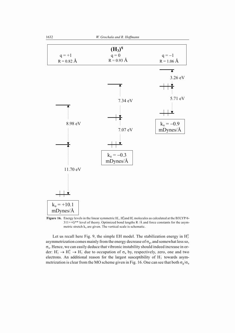
Let us recall here Fig. 9, the simple EH model. The stabilization energy in H30
asymmetrization comes mainly from the energy decrease of �g, and somewhat less so,�u. Hence, we can easily deduce that vibronic instability should indeed increase in or-der: H3
� H30 � H�
due to occupation of �u by, respectively, zero, one and twoelectrons. An additional reason for the largest susceptibility of H3
towards asym-metrization is clear from the MO scheme given in Fig. 16. One can see that both �g/�u
1632 W. Grochala and R. Hoffmann
8.98 eV
11.70 eV
7.07 eV
7.34 eV
ku = +10.1mDynes/Å
ku = 0.3mDynes/Å
ku = 0.9mDynes/Å
3.26 eV
5.71 eV
(H3)q
q = +1 q = 0 q = 1R=0.82 Å R=0.93 Å R=1.06 Å
Figure 16. Energy levels in the linear symmetric H3 , H3
0and H3 molecules as calculated at the B3LYP/6-
311++G** level of theory. Optimized bond lengths R /Å and force constants for the asym-metric stretch ku are given. The vertical scale is schematic.
R = 0.82 Å R = 0.93 Å R = 1.06 Å

and �u/� g* gaps decrease strongly with increase of negative charge on H3 skeleton.
This means – as a perturbation theoretic approach tells us – that vibronic second ordereffects will be strongest in the H3
case.The instability order H3
+ < H30 < H3
we have obtained and understood for H3 spe-cies might be transformed into a more general proposition: electron rich moleculeswill be more unstable towards asymmetrization than the corresponding electron-deficient molecules. Unfortunately, this simple rule is not generally valid. Considerfor example the F3
+ � F30 � F3
series. F30 is unsymmetrical, while there is strong theo-
retical and experimental evidence that a linear F3 molecule is symmetric [54]. How
could one explain this?We tend to think about relative stability of linear symmetric F3
molecule in termsof s-p mixing. Although s-p mixing will be the subject of the next section, let usshortly explain its role here (see Figs. 17 and 18 for details). For F3
s-p mixing showsup through a nonzero contribution of a 2s orbital to SOMO. This makes SOMOantibonding with respect to neighboring F atoms. Subsequently, symmetric elonga-tion of the F–F bonds will be driven by a greater force in F3
as compared to F30 . Having
in mind the general rule that G is more negative for shorter bonds, we might qualita-tively understand the stability trend in the F3 series. The more diffuse character of F3
orbitals (as compared to F30 ) and the larger polarizability also contribute to the
symmetrization of the F3 molecule.
2.4. Hybridization, s-p Mixing and Vibronic Coupling.
To understand the interplay of hybridization and s-p mixing in vibronic effects wewill use again a simple model based on EH considerations. We analyze the vibronicstability of a linear symmetric F3 molecule, varying the extended Hückel Hii of the 2sorbital of the central F atom (the Hii of the 2p orbital remains constant). This way wewill “steer” the s-orbital contribution to the three center bond orbitals and pass contin-uously from a 3 AO scheme (three 2p orbitals [55]) to a 4 AO one (one 2s and three 2porbitals). Fig. 17 shows the calculated plot of ku versus the difference of Hii betweenthe 2s and 2p orbital of the central F atom (� Hii (sp)). Negative � Hii (sp) means that2s orbital is below the 2p one.
The shape of the ku versus � Hii (sp) dependence is very interesting. Apparently,there is a huge vibronic stability decrease in the region of strong s-p mixing. Interest-ingly, the largest instability is observed for � Hii (sp) � 2 and not for � Hii (sp) = 0. Ofcourse, the region of positive � Hii (sp) corresponds to a very unphysical situation (sorbital above p) and we do not pay much attention to it. We are doing these numericalexperiments not to model a real molecule, but as a kind of laboratory to turn on s,pmixing, spanning the range from little mixing to much.
In the reasonable range of negative � Hii (sp), the important results is that thesmaller the s-p gap, the larger the vibronic instability.
Chemistry of vibronic coupling... 1633

We will now use a MO picture to explain the trend observed in Fig. 17.The three-center system built of p orbitals at each atom (and interacting s orbitals)
is a little different than the previously studied three s orbital system, so some intro-duction is needed. Fig. 18 shows the relevant orbitals before s-p mixing [56].
1634 W. Grochala and R. Hoffmann
-0.6
-0.5
-0.4
-0.3
-0.2
-0.1
0
0.1
0.2
-30 -20 -10 0 10 20
diff. Hii (sp) /eV
ku
/arb
.u.
� Hii (sp) / eV
Figure 17. Plot of the force constant for the antisymmetric stretch (ku) versus the difference of extendedHückel Hii parameter between the 2s and 2p orbital of the central F atom (� Hii (sp)), in thelinear symmetric F3 molecule. The theoretical results derive from an EH calculation.

Note that the SOMO is now �g in symmetry (and not �u as in the three s orbitalcase we studied earlier). The s orbital at the central atom has the same �g symmetry.The MO diagram is instructive for it tells us that the two �g orbitals (the low lying sand the SOMO) must interact, as long as there is any overlap between them. The netresult will be a “repulsion” of the orbitals, the lower one will be Fcenter/ Fright and Fcenter/ Fleft
bonding, the upper antibonding. This is why we label them even here as �g and � g* .
Chemistry of vibronic coupling... 1635
-14.4 eV
-18.1 eV
-19.7 eV
-25.1 eV
�u*
�g*
�u
�g
Figure 18. The MOs scheme of the linear symmetric F3 system before turning on the s-p mixing for Fcenter.The case shown is for a 2s–2p gap of –7 eV. Two different shades of gray represent oppositephases of wavefunction.

Fig. 19 shows the evolution of the �-block of MOs in the vicinity of the SOMO forthe linear symmetric F3 molecule, as the extended Hückel Hii for the 2s orbital of thecentral F atom is varied.
Analyzing Fig.19, we find the reasons for a strong dependence of the vibronic sta-bility on the s-p mixing. Our analysis takes into account only the four � orbitals in thevicinity of SOMO contributing substantially to the vibronic coupling along Qas: �g,�u, � g
* , � u* (see Fig. 18). The �-block of MOs does not mix with the s orbital of Fcenter
due to symmetry [57]. Moreover, the contribution from the � orbitals (mixing them-selves within � block) to the total vibronic coupling along Qas is much smaller thanthat from �.
It is clear from Fig. 19 that sp-hybridization plays important role in the vibroniccoupling: admixture of the s orbital of Fcenter into� g
* increases significantly the energychanges associated with asymmetrization. The reasons for this in the case of F3 are thefollowing:
i) the 2s orbital of Fcenter mixes into SOMO (� g* ) in an antibonding way;
ii) following such mixing, the energy gap between� g* and� u
* decreases, and thecontribution of the s orbital of Fcenter to � g
* increases. This, in turn, enablesmore efficient� g
* /� u* mixing after symmetry breaking (recall that such mixing
is turned on for Qas � 0);iii) asymmetrization effectively creates sp hybrids at Fcenter.Hence, the sp-mixing increases strongly the vibronic coupling in the � Hii (sp) < 0
region. The more distant (in energy) the lower-lying (occupied) 2s orbitals from the �2p orbitals, the larger the vibronic stability. This finding is in general agreement withwhat is known of the influence of s-p mixing on vibronic stability in many extendedstructures [58].
Let us now investigate the relationship of the s-p mixing to “ionic/covalent”curve crossing, and analyze the importance of the latter for vibronic coupling.
2.5. Avoided “Ionic/Covalent” Curve Crossing and the Vibronic Coupling.
The results presented in the previous section may also be interpreted using a lan-guage of ionic/covalent curve crossing.
It is clear from Fig. 19 that a “repulsion” of the �g orbitals occurs in the pseudo–F3
molecule as the extended Hückel Hii of the 2s orbital of the central F atom is varied(Hii of the 2p orbital remains constant). This is emphasized by dotted curves in Fig.19a. Both �g orbitals significantly change their character as a result. The lower energy�g orbital is dominated by a 2s contribution of the central F atom for � Hii (sp) = –7 eV,and by a 2p contribution of the side F atoms for � Hii (sp) = +7 eV. The reverse is truefor the higher energy � g
* orbital. Clearly, a kind of curve crossing has taken place inthis system.
We emphasize again that the region with 2s close to and especially above 2p isunphysical. Nevertheless, variation of the 2s-2p energy difference over a large range
1636 W. Grochala and R. Hoffmann

Chemistry of vibronic coupling... 1637
Figure 19b. Evolution of the MOs of the linear symmetric F3 system upon varying the extended HückelHii parameter for the 2s orbital of the central F atom. The cases shown are for a 2s–2p gap(� Hii (sp)) of –7 eV, 0 eV and +7 eV.
-24.8
-16.9
-19.7
-14.4 eV�u*
�u
�g
7 eV 2 eV 0 eV +2 eV +7eV
� Hii (sp) =
-20.6
-19.7
-16.3
-14.4
-19.7
-19.5
-15.5
-14.4
-19.7-19.7
-14.4
-14.2
-18.8-18.3
-14.4
-9.9
�g*
� Hii (sp) =
7 eV 0 eV +7 eV
Figure 19a. Evolution of the MOs scheme of the linear symmetric F3 system upon varying the extendedHückel Hii parameter for the 2s orbital of the central F atom. The cases shown are for a 2s–2pgap (� Hii (sp)) of –7 eV, –2 eV, 0 eV, +2 eV and +7 eV. For more details see text. “Repulsion”of the �g levels is illustrated schematically with dotted lines. Energy in eV.
�g*
�g
�u
�u*
�g*
�g
�u
�u*
E/eV
SOMO
eV

is a useful way to tune s,p mixing. And this is what different elements in the periodictable do – vary the ns-np energy difference, even if ns is never above np.
Let us elaborate our argument for saying a curve crossing has taken place. Varia-tion of the extended Hückel Hii of the 2s orbital of the central F atom influences theelectronegativity of the central F atom. The computed Mulliken charge on the centralF atom is +0.30 e for � Hii (sp) = –7 eV, and as much as +1.51e for � Hii (sp) = +7 eV. Itis a typical feature of the 4-electron hypervalent AAA systems that the central atom ispositively charged relative to the end atoms [59]. A chemist is likely to assign elec-tron occupation in the F–F–F system as:
s2p5, s2p5, s2p5 or F0–F0–F0 for � Hii (sp) = –7 eV (5)
and
s2p6, s0p3, s2p6 or F–1–F+2–F–1 for � Hii (sp) = +7 eV (6)
In other words, the “forbidden curve crossing” has the character of a “cova-lent–to–ionic transition“! And it enormously influences the vibronic stability of amolecule, as we have seen.
At this point two interesting and important theoretical contributions to the litera-ture come to mind. In these the authors link the superconductivity phenomenon in thesolid state either to “sudden polarization as a result of small geometrical distortion”(hypothetical organic superconductors, Salem 1966) [60], or directly to “ionic/cova-lent curve crossing” (oxocuprate materials, Burdett 1993) [2s].
In particular, Burdett discussed in some detail the possible influence of the“ionic/covalent curve crossing” on the “magic electronic state” in oxocuprate super-conductors. He postulated that there are huge variations of the wavefunction withCu–O distance in the “ionic/covalent curve crossing” region:
Cu3+ + O2– � Cu2+� + O–� (7)
We feel that Burdett’s hypothesis is of a particular importance for theoreticalstudies of the electronic structure of superconducting materials. The existence of acurve crossing region might lead to large variations in the nature of the computedwavefunction for the system, which might be forced towards either “ionic” or “cova-lent” configurations.
We have computed the vibronic stability of a symmetric linear [Cu3+–O2––Cu2+]�
species along an antisymmetric stretching coordinate, using EH. We have varied Hii
for the p orbital of the central O atom in a broad energy range so to model avoidedcrossing with Cu(d) orbitals; the procedure (and purpose) is analogous then to thatapplied for a pseudo-F3 model. Varying O(p) orbital energy allows us tune Cu(d)/O(p)orbital mixing. Such mixing is known to occur in oxocuprate materials, and certainly
1638 W. Grochala and R. Hoffmann

depends on the oxidation state of Cu. Strong increase in vibronic instability has beencomputed in the vicinity of the crossing region, as compared to the region whereCu(d)/O(p) mixing is small. While the increase was not as steep a function of Hii as forthe pseudo-F3 molecule, yet the essence of the phenomenon was preserved.
Burdett’s and Salem ideas can be transferred to the BCS theory of superconduc-tivity [61]. States below and above the Fermi level, which are coupled in pairsthrough an optical phonon, are now in the “forbidden curve crossing region”, andtheir coupling increases significantly. In this paper we have argued that “ionic/cova-lent curve crossing” dramatically influences the vibronic stability of a molecule [62].An analogue of Burdett’s idea thus is found for triatomic molecules, even at the ex-tended Hückel level [63].
2.6. Vibronic Coupling and Resonance Structures.
Consider another approach to vibronic coupling. Let us think in terms of reso-nance structures, an archetypical concept in chemical language. Lines in resonancestructures symbolize spin–coupled electron pairs localized in bonds or in lone pairs.Resonance structures are a classic tool that chemists use to describe qualitatively theelectron distribution of molecules. Valence bond theory, in which the “resonancestructures” terminology originates, also is the basis of a curve–crossing model [64].Resonance structures and valence bond configurational thinking has been very suc-cessfully applied by Shaik and coworkers to studies of dynamics of the chemical reac-tions and properties of transition states. The quantitative approach presented in [64]allows a beautiful connection to be made between a singlet-triplet gap in A2 diatomicsand the gap between “repulsive” potential energy curves of symmetric A3 triatomics.Inclusion of a low lying ligand-to-metal charge-transfer state increases the stabilityof a symmetric (“ionic”) transition state and lowers the energy barrier for an A + BA� AB + A reaction.
We think that the studies of Shaik and coworkers are very much relevant to the de-scription of systems exhibiting large vibronic coupling. It also becomes clear nowwhy large vibronic coupling in T1 states of interhalogen AB molecules [4] is likely toimply strong vibronic instabilities in interhalogen ABA open-shell systems [5].
CONCLUSIONS
We have concentrated our attention on the off-diagonal vibronic coupling. Wehave examined off-diagonal vibronic coupling in symmetric linear triatomic A2Bopen-shell molecules, for the antisymmetric stretching mode. The triatomic A2Bmolecules are usually classified into two groups: mixed-valence (MV) and interme-diate-valence (IV) (using criteria of static/dynamic nonequal/equal charge distribu-tion on two centers A), and they are ideal for studying vibronic coupling.
The vibronic stability of ABA molecules (as measured by the force constant ofthe antisymmetric stretching mode, ku, as well as the “antisymmetric mode softening
Chemistry of vibronic coupling... 1639

parameter” G) has been studied. G is defined as the ratio of antisymmetric to symmet-ric stretching force constant; it is a very sensitive indicator of vibronic coupling. Inthis paper the range of A, B is very wide – element B originated from s, p, and A froms, p and d-blocks of the periodic table.
We have constructed maps of G in a space of two parameters: the difference of thePauling electronegativity of A and B elements constituting A2B molecule and the sumof the Pauling electronegativity for A and B. Alternatively, we have used the parame-ter f (f is defined as sum of electronegativities divided by AB bond length) instead ofthe sum of electronegativities. Our maps show that there exists a region of strongvibronic instability of A2B molecules. This is observed for large values of f which arecharacteristic for small ABA molecules built of two nonmetallic p-block elements.ABA molecules containing a d-block element A are usually more vibronically stablethan analogous molecules containing a p-block A element of same electronegativity.
Another interesting result of relevance to the vibrational spectra of A2B mole-cules (see Appendix A) has been obtained: it appears that f correlates with the forceconstant for the symmetric stretching mode in certain families of linear symmetrictriatomics.
Trying to rationalize the trends observed for h egi in the space of certain “chemical”
parameters, we constructed simple MO models, based on EH and DFT computations.We discuss h eg
i in A2B molecules in relevance to hypervalence, s-p mixing, “ionic/co-valent curve crossing”, and the hardness/softness of Lewis acids/bases. The most im-portant general conclusions are the following:
i) Molecular systems built of hard Lewis acids/bases should be vibronicallymore unstable than systems built of soft Lewis acids/bases [65].
ii) The more pronounced s-p mixing, the larger the vibronic instability.iii) An “ionic/covalent curve crossing” significantly increases the vibronic insta-
bility of a molecule.Vibronic instability may be significant (i.e. may lead to geometrical instability of
symmetrical molecular systems, with consequences for various observables) even formolecules with large energy gaps of about 10–15 eV (as in the case of the ammonia in-version [18]). The vibronic effects are most significant when states mixed (which arenot necessarily nearest in energy) involve strongly bonding or antibonding orbitals
(bonds are strongly weakened and/or strengthened during the molecular vibration). Itis also known that vibronic effects are extremely important in both “classical” BCS[1] and high-temperature superconductivity [2]. In this paper we tried to show whatmight be the conditions for large vibronic instability [66].
Our theoretical findings may be important in the experimental search for newsuperconducting materials in solid state. It is still a long way from simple physicalmodels and quantum mechanical computations for small molecules to the complexbehavior of solids due to their collective electronic / magnetic phenomena. We willtry to come part of this way in our next paper [5].
1640 W. Grochala and R. Hoffmann

Acknowledgments
This research was conducted using the resources of the Cornell Theory Center, which receives fundingfrom Cornell University, New York State, the National Center for Research Resources at the National Insti-tutes of Health, the National Science Foundation, the Defense Department Modernization Program, theUnited States Department of Agriculture, and corporate partners. We were supported by the Cornell Centerfor Materials Research (CCMR), a Materials Research Science and Engineering Center of the National Sci-ence Foundation (DMR-9632275) and by NSF Research Grant (CHE 99-70089). Authors acknowledge Nor-man Goldberg and Mihaela Bojin for helpful comments.
Appendix A
Utility of f for Predicting kg.The qualitative correlation of parameter f with the force constant for the symmetric stretching mode
(kg) was discovered by us previously, for three families of ABA� triatomics: intermetallics, interhalogensand salts [5,67]. We may elaborate a quantitative approach, based on the extensive calculations of this pa-per. Fig. 20 presents the plot of �kg versus parameter f for about 100 previously studied AB2
� molecules [5].There is a good monotonic correlation between �kg and f. The least square linear relationship found
is: �kg = 0.344 f + 0.166, with correlation coefficient R2 = 0.909. Thus f correlates sufficiently well with
Chemistry of vibronic coupling... 1641
0
0.5
1
1.5
2
0 1 2 3 4 5 6
f / arb. u.
kg
1/2
k(g) vs fkg1/2
vs f
Figure 20. Linear least – squares correlation between �kg and parameter f for a broad family of about 100linear symmetric triatomic radicals (AB2
�). The least-squares fitted linear curve is shown withdotted line.

the square root of the second derivative of the potential energy (i.e. force constant) [28]. We obtained alsoa good �kg vs f correlation for all 460 molecules studied in this paper (including those containing transi-tion metal atoms). Note that f also correlates well with the first derivative of the potential energy (i.e.force) in certain families of diatomics [4]. It is impressive to us that a simple empirical parameter corre-lates so well with the results of complex quantum mechanical computations [68]. We think that f willprove useful for analyzing other molecular features as well.
Appendix B
Basis Set Effects in Vibronic Coupling – a DFT Picture.There is another, indirect way to look at the role of softness and hardness in affecting vibronic stabil-
ity. Let’s look at the influence of the basis set on the vibronic stability parameter G. We have chosen H2Clas a subject of this study.
Adding polarization and diffuse function to the basis set on one hand is just an applied mathematicalprocedure to get a more accurate solution of the wave equation. But, we think that there is something phys-ical and chemical to be learned from the effects of polarization and diffusion functions. Such basis setfunctions are especially important for systems with diffuse or low lying unoccupied orbitals. Electrons insuch systems are usually easily polarizable and weakly bound. We think that one way to judge that a sys-tem is “hard” is if little addition of polarization and diffuse function to the basis set is necessary to de-scribe it properly.
In Table 1 we list optimized bond length R0, force constants for symmetric (kg) and antisymmetric(ku) stretching modes and vibronic stability parameter G for H2Cl as computed at B3LYP level with differ-ent basis sets.
Table 1. Influence of the basis set choice on the optimized bond length R0, force constants for symmetric (kg)and antisymmetric (ku) stretching modes and vibronic stability parameter G for H2Cl as computed atDFT/B3LYP level.
basis set R0/Å ku/mdyne Å–1 kg/mdyne Å–1G/1
6-311++G** 1.50 –0.90 1.99 –0.45
6-31++G** 1.50 –0.91 1.99 –0.46
6-31+G** 1.50 –0.92 1.99 –0.47
6-31G** 1.50 –0.91 2.00 –0.45
6-31G* 1.51 –1.01 1.87 –0.54
6-31G 1.56 –0.96 1.64 –0.59
6-21G* 1.51 –1.05 1.82 –0.58
6-21G 1.57 –0.98 1.56 –0.63
4-31G* 1.52 –1.15 1.76 –0.65
4-31G 1.57 –0.98 1.58 –0.62
3-21G* 1.51 –1.08 1.76 –0.62
3-21G 1.57 –1.00 1.52 –0.66
It may be immediately seen from Table 1 that basis set choice has a small effect on the optimizedbond length, but a substantial one on the parameter G for the symmetric linear H2Cl molecule. We ob-tained the largest vibronic instability (G = –0.66) with the smallest basis set (3-21G), and the smallestvibronic instability (G = –0.45) with the largest basis set (6-311++G**). G increases upon inclusion ofpolarization functions (6-31G � 6-31G* � 6-31G**). The same is true for other families of basis sets.Apparently, progressive addition of polarization functions results in a decrease of the vibronic instability.
1642 W. Grochala and R. Hoffmann

How G varies upon addition of diffuse functions is not very clear, nor as significant in the case ofH2Cl as for polarization functions. For basis sets: 6-31G**, 6-31+G**, and 6-31++G** we obtain G equalto –0.45, –0.47, and –0.46, respectively. The vibronic stability (G) changes only slightly upon progressiveaddition of diffuse functions.
The influence of the basis on computed G is substantial; the ratio of the smallest and the largest com-puted G value is large (~150%). Of course, linear H2Cl is strongly vibronically unstable, so even a basisset that is too small does not result in a qualitative error (for all basis sets G << 0). However, one may eas-ily imagine cases for G � 0, when an improper choice of basis might be the source of serious qualitative(stability or instability?) error.
We suggest that vibronic coupling is likely to be large in systems built of atoms for which addition ofpolarization and diffuse function to the basis set only slightly influences the computed vibronic stabilityparameters (i.e. of small, weakly polarizable atoms). Results of the above study may be thus nicely relatedto conclusions from section 2.2.
REFERENCES
1. Bardeen J., Cooper L.N. and Schrieffer J.R., Phys. Rev., 108, 175 (1957).2. On the importance of vibronic effects (and generally: lattice–electron coupling) for superconductivity
see: (I) oxocuprates: (a) Alexandrov A.S. and Edwards P.P., Physica C, 331, 97 (2000), and referencestherein. (b) Burdett J.K. and Kulkarni G.V., Phys. Rev. B, 40, 8908 (1989). (c) Jarlborg T., Solid State
Commun., 67, 297 (1988). (II) oxobismuthates: (d) Meregalli V. and Savrasov S.Y., Phys. Rev. B, 57,14453 (1998). (e) Navarro O. and Chavira E., Physica C, 282–287, 1825 (1997). (f) Shirai M., Suzuki N.and Motizuki K., J. Phys.: Condens. Matter., 2, 3553 (1990). (III) fullerides: (g) Schluter M., Lanoo M.,Needels M., Baraff G.A. and Tomanek D., Phys. Rev. Lett., 68, 526 (1992). (h) Jishi R.A. andDresselhaus M.S., Phys. Rev. B, 45, 2579 (1992). (i) Novikov D.L., Gubanov V.A. and Freeman A.J.,Physica C, 191, 399 (1992). (j) Kresin V.Z., Phys. Rev. B, 46, 14883 (1992). (k) Asai Y. and KawaguchiY., Phys. Rev. B, 46, 1265 (1992). (l) Rai R., Z. Phys. B, 99, 327 (1996). (IV) silicide clathrates: (m)Yoshizawa K., Kato T. and Yamabe T., J. Chem. Phys., 108, 7637 (1998). (n) Yoshizawa K., Kato T.,Tachibana M. and Yamabe T, J. Phys. Chem. A, 102, 10113 (1998). (V) borocarbides: (o) Gompf F.,Reichardt W., Schober H., Renker B. and Buchgeister M., Phys. Rev. B: Condens. Matter., 55, 90581997). (VI) mercury fluoroarsenates: (p) Slot J.J.M., Boon M. and Weger M., Solid State Commun., 56,645 (1985). On accuracy of BCS predictions for different classes of superconductors see: (r) B.Chakraverty, Ramakrishnan T., Physica C, 282–287, 290 (1997). On the “magic electronic state” inoxocuprates and its connection to Cu-O bond stretching see: (s) Burdett J.K., Inorg. Chem., 32, 3915(1993).
3. Part 1, Grochala W., Konecny R. and Hoffmann R., Chem. Phys., 265, 153 (2001).4. Part 2, Grochala W. and Hoffmann R., New J. Chem., 25, 108 (2001).5. Part 3, Grochala W. and Hoffmann R., J. Phys. Chem. A, 104, 9740 (2000).6. In some sense our paper is analogous to the review on periodicity in 120 first- and second-row diatomic
molecules, by Boldyrev A.I., Gonzales N. and Simons J., J. Phys. Chem., 98, 9931 (1994).7. Part 5, Grochala W., Hoffmann R. and Edwards P.P., manuscript in preparation.8. Gaussian 94, Revision D.3, Frisch M.J., Trucks G.W., Schlegel H.B., Gill P.M.W., Johnson B.G., Robb
M.A., Cheeseman J.R., Keith T., Petersson G.A., Montgomery J.A., Raghavachari K., Al-Laham M.A.,Zakrzewski V.G., Ortiz J.V., Foresman J.B., Cioslowski J., Stefanov B.B., Nanayakkara A.,Challacombe M., Peng C.Y., Ayala P.Y., Chen W., Wong M.W., Andres J.L., Replogle E.S. , GompertsR., Martin R.L., Fox D.J., Binkley J.S., Defrees D.J., Baker J., Stewart J.P., Head-Gordon M., GonzalezC. and Pople J.A., Gaussian, Inc., Pittsburgh PA, 1995.
9. HyperChem 5.0, Hypercube, Inc. Ltd.10. Landrum G.A.,”YAEHMOP: Yet Another extended Hückel Molecular Orbital Package.” A package for
performing EH calculations on molecules and extended systems and visualizing the results. (1995)YAeHMOP is freely available for both Unix workstations and Power Macintosh systems on the WWWat URL http://overlap.chem.cornell.edu:8080/yaehmop.html.
Chemistry of vibronic coupling... 1643

11. C.A.C.A.O. (Computer Aided Composition of Atomic Orbitals), A Package of Programs for MolecularOrbital Analysis [PC Beta-Version 5.0 , 1998], Mealli C. and Proserpio D.M., with a major contributionby Ienco A., J. Chem. Educ., 67, 399 (1990).
12. The reader is referred to several classical texts on vibronic coupling in triatomic and multiatomic mole-cules, whose importance was brought to our attention by a reviewer: (a) Öpik U. and Pryce M.H.L., Proc.
Roy. Soc. A, 238, 425 (1957); (b) Bader R.F.W., Mol. Phys., 3, 137 (1960); (c) Bader R.F.W., Canad. J.
Chem., 40, 1164 (1962); (d) Köppel H., Domcke W., and Cederbaum L.S., Adv. Chem. Phys., 57, 59(1984); (e) Bersuker I.B. and Polinger V.Z., Vibronic Interactions in Molecules and Crystals, Springer-Verlag: Berlin, 1989; (f) Wong K.Y. and Schatz P.N., A Dynamic Model for Mixed-Valence Compounds.Progress in Inorganic Chemistry, vol. 28; Lippard S.J. Ed.; John Wiley and Sons: NY 1981; p.369; (g)Bersuker I.B., The Jahn-Teller Effect and Vibronic Interactions in Modern Chemistry, Plenum Press: NY1984. Theoretical models accompanied by calculations of vibronic stability for some “real” organic andinorganic molecules are presented in these papers.
13. As shown in Table S2 in Supplement, we could not compute 8 of 100 molecules in this family. The rea-sons for failure varied: problems with convergence, failures of Coulomb series, and density matrixbreaking symmetry problems.
14. As shown in Table S2 in Supplement, we also could not compute 29 of the additional 240 molecules inthis family. The reasons, as mentioned in Ref. 13, varied.
15. (a) Murphy L.R., Meek T.L., Allred A.L. and Allen L.C., J. Phys. Chem. A, 104, 5867 (2000). (b) CaoC.Z., Li Z.L. and Allen L.C., Chin. J. Inorg. Chem., 15, 218 (2000). On configuration energies, a modernconcept related to electronegativity, see for example: (c) Mann J.B., Meek T.L. and Allen L.C., J. Am.
Chem. Soc., 122, 2780 (2000). (d) Mann J.B., Meek T.L., Knight E.T., Capitani J.F. and Allen L.C., J.
Am. Chem. Soc., 122, 5132 (2000).16. Pauling L., J. Am. Chem. Soc., 54, 3570 (1932).17. Luo Y.-R. and Benson S.W., J. Phys. Chem., 94, 914 (1990).18. Khadikar P.V. and Pandharkar S., Japan. J. Appl. Phys., 27, 2183 (1988).19. Thomas T.D., J. Am. Chem. Soc., 92, 4184 (1970).20. Prasad P.L. and Singh S., J. Chem. Phys., 66, 162 (1977).21. Han W.-P. and Ai M., J. Catalysis, 78, 281 (1982).22. (a) Van Arkel A.E., Molecules and Crystals in Inorganic Chemistry; Interscience: NY, 1956.
(b) Ketlaar J.A.A., Chemical Constitution, An Introduction to the Theory of the Chemical Bond, 2nd ed.,Elsevier: NY, 1958.
23. (a) Timoten R.S., Seetula J.A., Niiranen J. and Gutman D., J. Phys. Chem., 95, 4009 (1991). (b) SchaeferT. and Hutton H.M., Canad. J. Chem., 45, 3153 (1967). (c) Davies A.G., Smith L. and Smith P.J., J.
Organomet. Chem., 23, 135 (1970).24. (a) Parr R.G. and Pearson R.G., J. Am. Chem. Soc., 150, 7512 (1983). For the maximum hardness princi-
ple, see, for example: (b) Pearson R.G., J. Chem. Educ., 76, 267 (1999).25. (a) Gázquez J.L, J. Phys. Chem. A, 101, 9464 (1997). (b) Pearson R.G., J. Am. Chem. Soc., 110, 7684
(1988).26. Mooser E. and Pearson W., Acta Crystallogr., 12, 1015 (1959).27. Shankar S. and Parr R.G., Proc. Natl. Acad. Sci. USA, 82, 264 (1985).28. The Pauling electronegativity (PEN) has been used in this paper to compute f. Since PEN has formally
units of square root of energy, f has units of square root of energy per distance. This might explain why acorrelation of f with square root of the force constant (see Fig. 12) is almost linear (square root of forceconstant also has square root of energy per distance units). There is another electronegativity definition,the Mulliken electronegativity (MEN, expressed in energy units). MEN correlates quite well with PENfor most of elements. f would formally have energy per distance, i.e. force units if one defined f usingMEN. Note that we obtained a strongly nonlinear correlation between f and force in Ref. 4.
29. Pearson R.G., J. Molec. Struct., 300, 519 (1993).30. As far as we know, there is no experimental data available for the symmetric linear radicals investigated
in this paper. Such radicals are often not bound, and dissociate to a diatomic and an isolated atom. Thespecies studied here might also be intermediates or transition states between two asymmetric linear, ortwo symmetric bent minima (these minima would correspond to “real” ground state molecules). Ourstudy is not intended to predict the geometry of molecular radicals, but to discern trends in vibronic cou-pling.
1644 W. Grochala and R. Hoffmann

31. Dissociation of symmetric linear triatomic proceeds along a combination of antisymmetric and symmet-ric stretching coordinates. In this paper we study the potential energy surface of a triatomic along anantisymmetric stretching coordinate, with symmetric stretching coordinate optimized and then frozen.
32. This study does not include closed–shell linear symmetric triatomics, such as e.g. CO2. The presence ofan unpaired electron in the species studied here usually results in strong vibronic coupling in these sys-tems, in contrast to the closed–shell ones.
33. An unequal distribution of points in the ABA and BAB regions contributes partially to the left-rightasymmetry of Fig. 3, but is not its main cause.
34. It has to be mentioned that kg for all triatomics investigated in this paper also correlates very well with f.35. Haddon R.C., Acc. Chem. Res., 25, 127 (1992).36. (a) Mattheiss L.F. and Hamann D.R., Phys. Rev. Lett., 60, 2681 (1988). (b) Cava R.J., Batlogg B.,
Krajewski J.J., Farrow R., Rupp L.W., White A.E., Short K., Peck W.F. and Kometani T., Nature, 332,814 (1988).
37. Bednorz J.G. and Müller K.A., Z. Phys. B, 64, 189 (1986).38. Yamanaka S., Hotehama K. and Kawaji H., Nature, 392, 580 (1998).39. As Table S2 details, we could not compute properly 24 among 120 molecules in this group.40. The only exception is Ir2Li, which surprisingly is computed to be vibronically unstable.41. Bally T. and Borden W.T., Calculations on Open-Shell Molecules: A Beginner’s Guide, Rev. Comput.
Chem., vol. 13, Lipkowitz K.B., Boyd D.B., Eds.; John Wiley and Sons: NY, 1999, p.1.42. The difference of extended Hückel Hii between 5s of Cs and 2p of F is about 15 eV, except F bonding is
mainly through 2p.43. Hoffmann R., Acc. Chem. Res., 4, 1 (1971).44. A general perturbation theory for a one–electron LCAO-MO method, including change of the overlap
integrals, has been developed by Imamura (Imamura A., Mol. Phys., 15, 225 (1968)).45. We will discuss this point further in Ref. 7.46. Parr R.G. and Pearson R.G., J. Am. Chem. Soc., 105, 1503 (1983).47. Pearson R.G., Inorg. Chem., 27, 734 (1988).48. We note that our results agree well with recent data on vibronic stability of planar triangular closed-shell
AX3 molecules (A = N to Bi, X = H, F to I): (a) Atanasov M. and Reinen D., J. Phys. Chem. A, 105, 5450(2001); (b) 15th International Jahn-Teller Symposium “Vibronic Interactions in Crystals and Molecules”,Boston, 2000, Atanasov M. and Reinen D., Chem. Eur. J., submitted. The authors conclude that the hard-est molecules are the most susceptible to vibronic coupling (hardness is used by them in the chemicalsense of Pearson’s hardness �).
49. Ayers P.W. and Parr R.G., personal communication, 2000.50. Some people see red when “hypervalence” is mentioned. We find this term to be heuristically useful and
use it interchangeably with three–center four–electron bonding.51. (a) Feretti V., Gilli P., Bertolasi V. and Gilli G., Crystallogr. Rev., 5, 3 (1996); (b) Bürgi H.-B. and Dunitz J.D.,
Eds. Structure Correlation, vol. 1; VCH: Weinheim, 1994; (c) Akiba K., Chemistry of Hypervalent Com-
pounds; Wiley – VCH: NY, 1999, Chapter 1; (d) Musher J.I., Angew. Chem. Int. Ed. Engl., 8, 54 (1969).52. A formal negative sign has been introduced for the force constant if the corresponding computed fre-
quency is imaginary.53. Of course, H3
+ wants to be triangular. But in the spirit of our studies we keep it linear here.54. (a) Cahill P.A., Dykstra C.E. and Martin J.C., J. Am. Chem. Soc., 107, 6359 (1985). (b) Novoa J.J., Mota
F. and Alvarez S., J. Phys. Chem., 92, 6561 (1988). (c) Ault B.S., Andrews L., Inorg. Chem., 16, 2024(1977). (d) Landrum G.A., Goldberg N. and Hoffmann R., J. Chem. Soc., Dalton Trans., 3605 (1997).
55. We use here an approximate (three p orbitals) instead of a more correct picture (three p orbitals + two sorbitals at Fleft and Fright), since the s–p mixing at Fleft and Fright is relatively small, and not relevant to ourdiscussion.
56. There is some s-p mixing at the terminal F’s, which “shapes” these orbitals a little.57. The s orbital of central F atom does contribute to the vibronic coupling along the normal coordinate for
bending, however.58. (a) Papoian G. and Hoffmann R., Angew. Chem. Int. Ed., 39, 2408 (2000); (b) Ienco A, Hoffmann R. and
Papoian G., J. Am. Chem. Soc., submitted.59. This might be the reason why the “negative peak” in Fig. 13 does not occur for �Hii (sp) = 0, but for some
positive value of �Hii (sp).
Chemistry of vibronic coupling... 1645

60. Salem L., Molec. Phys., 11, 499 (1966).61. It is significant that avoided crossing seems to be important for such different superconducting materials
as samarium sulphide, SmS (Varma C.M., Rev. Mod. Phys., 48, 218 (1976)) and oxocuprates (Ref. 2s).Independent calculations confirm the hypothesis of dual character of the wavefunction for oxobis-muthates, as well (Pyper N.C. and Edwards P.P., in: Polarons and Bipolarons in High-TC Superconduc-tors and Related Materials, ed. by Salje E.K.H, Alexandrov A.S. and Liang W.Y., Cambridge UniversityPress, Cambridge 1995).
62. One should consider in a more rigorous approach also nonadiabatic corrections, which are important inthe vicinity of curve–crossing region.
63. Of course, the model used by us to simulate “ionic/covalent curve crossing” may be substituted by otherapproaches. A rigorous model for an ABA triatomic should show how the “ionic/covalent curve cross-ing” along the symmetric stretching coordinate influences the vibronic stability along the antisymmetricstretching coordinate.
64. (a) Shaik S.S. and Shurki A., Angew. Chem. Int. Ed., 38, 586 (1999). (b) Maitre P., Hiberty P.C.,Ohanessian G. and Shaik S.S., J. Phys. Chem., 94, 4089 (1990).
65. Large vibronic instability for systems with deep lying, contracted orbitals suggests the potential utility ofa Hamilton population analysis (HP) for analysis of vibronic coupling (see for example HP vs Hii de-pendence in: Glassey W.V. and Hoffmann R., J. Chem. Phys., 113, 1698 (2000).
66. From both computations and theoretical models we know how to reach the goal of large vibronic cou-pling. However, there is a limit to the extent and significance of large vibronic coupling. This limit is de-termined by the thermodynamic stability of a molecule toward asymmetric dissociation. If the couplingis so large that it leads to an ABA molecule’s dissociation (such dissociation proceeds along a combina-tion of antisymmetric and symmetric stretching coordinates), then that coupling in a way has no realphysical importance. A linear symmetric structure (the point at which G is determined) is then too faraway from any real equilibrium geometry. Hence, “prodissociative”, enormously large coupling con-stants might not be useful in pointing to molecules which may have interesting properties.
67. The increase of the experimental force constants in the order I2 < Br2 < Cl2 < F2, Rb2 < K2 < Na2 < Li2, andHI < HBr < HCl < HF, has been noted, and an interesting correlation of the force constants with dissocia-tion energies has been introduced (Nakamoto K., Infrared and Raman Spectra of Inorganic and Coordi-nation Compounds, 3rd Ed., John Wiley and Sons: NY, Chichester, Brisbane, Toronto, 1978).
68. We have made some progress toward a physical justification of the use of f; this work will be publishedelsewhere.
Supplement – Tables
Table S1. Calculated geometric, vibrational and vibronic parameters for linear ABA� molecules where A, B= s, p – block element: optimized A–B bond length (R0/Å), force constant for the symmetric(kg/mDyne Å–1) and antisymmetric stretching (ku/mDyne Å–1), and vibronic stability parameter(G/1). Sum and difference of electronegativities between A and B (ENA + ENB, and � EN, respec-tively), parameter f [arb.u.], difference of Hückel parameters for A and B valence orbitals (�EHückel/eV), and �kg (arb.u.) are also shown. Molecules are grouped following main groups of theperiodic table. Negative values of ku and G indicate imaginary frequency for antisymmetric stretch.
molecule � EN ENA + ENB R0/Åkg/mDyne
Å–1ku/mDyne
Å–1 G/1f/
arb.u.�EHückel/
eV�kg/
arb.u
Group 1
H2F 1.9 6.1 1.149 2.562 –3.354 –1.31 5.31 4.5 1.60
H2Cl 0.9 5.1 1.500 1.991 –0.901 –0.45 3.40 0.6 1.41
H2Br 0.7 4.9 1.664 1.582 –0.747 –0.47 2.94 –0.5 1.26
H2l 0.4 4.6 1.809 1.410 –0.291 –0.26 2.54 –0.9 1.19
1646 W. Grochala and R. Hoffmann

Table S1 (continuation)
H3 0.0 4.2 0.931 2.510 –0.322 –0.13 4.51 0.0 1.58
H2Li –1.1 3.1 1.763 0.479 0.501 1.05 1.76 –8.2 0.69
H2Na –1.2 3.0 2.012 0.450 0.452 1.00 1.49 –8.5 0.67
H2K –1.2 3.0 2.434 0.298 0.313 1.05 1.23 –9.26 0.55
H2Rb –1.3 2.9 2.608 0.275 0.282 1.03 1.11 –9.42 0.52
H2Cs –1.4 2.8 2.799 0.245 0.259 1.06 1.00 –9.72 0.49
Li2F 3.0 5.0 1.682 1.366 2.714 1.99 2.97 12.7 1.17
Li2Cl 2.0 4.0 2.158 0.792 1.134 1.43 1.85 8.8 0.89
Li2Br 1.8 3.8 2.338 0.646 0.680 1.05 1.63 7.7 0.80
Li2I 1.5 3.5 2.562 0.512 0.455 0.89 1.37 7.3 0.72
Li2H 1.1 3.1 1.574 0.932 2.242 2.41 1.97 8.2 0.97
Li3 0.0 2.0 2.885 0.159 0.367 2.31 0.69 0.0 0.40
Li2Na –0.1 1.9 3.090 0.131 0.199 1.52 0.61 –0.3 0.36
Li2K –0.1 1.9 3.571 0.092 0.118 1.28 0.53 –1.06 0.30
Li2Rb –0.2 1.8 3.740 0.084 0.085 1.01 0.48 –1.22 0.29
Li2Cs –0.3 1.7 3.995 0.072 0.069 0.96 0.43 –1.52 0.27
Na2F 3.1 4.9 2.034 1.093 2.885 2.64 2.41 13.0 1.05
Na2Cl 2.1 3.9 2.524 0.575 1.289 2.24 1.55 9.1 0.76
Na2Br 1.9 3.7 2.690 0.502 0.822 1.64 1.38 8.0 0.71
Na2I 1.6 3.4 2.908 0.400 0.496 1.24 1.17 7.6 0.63
Na2H 1.2 3.0 2.01* *** 1.50 8.5
Na2Li 0.1 1.9 3.069 0.134 0.261 1.95 0.62 0.3 0.37
Na3 0.0 1.8 3.256 0.112 0.236 2.11 0.55 0.0 0.33
Na2K 0.0 1.8 3.723 0.081 0.168 2.07 0.48 –0.76 0.28
Na2Rb –0.1 1.7 3.884 0.074 0.111 1.50 0.44 –0.92 0.27
Na2Cs –0.2 1.6 4.138 0.066 0.087 1.32 0.39 –1.22 0.26
K2F 3.1 4.9 13.86
K2Cl 2.1 3.9 2.949 0.424 1.159 2.73 1.32 9.86 0.65
K2Br 1.9 3.7 3.096 0.385 0.921 2.39 1.20 8.76 0.62
K2I 1.6 3.4 3.348 0.299 0.578 1.93 1.02 8.36 0.55
K2H 1.2 3.0 2.46* 1.22 9.26
K2Li 0.1 1.9 3.552 0.089 0.161 1.81 0.53 1.06 0.30
K2Na 0.0 1.8 3.721 0.078 0.153 1.96 0.48 0.76 0.28
K3 0.0 1.8 4.223 0.055 0.115 2.09 0.43 0 0.23
Chemistry of vibronic coupling... 1647

Table S1 (continuation)
K2Rb –0.1 1.7 4.360 0.055 0.098 1.78 0.39 –0.16 0.23
K2Cs –0.2 1.6 4.613 0.046 0.069 1.50 0.35 –0.46 0.21
Rb2F 3.2 4.8 13.92
Rb2Cl 2.2 3.8 3.140 0.365 0.892 2.44 1.21 10.02 0.60
Rb2Br 2.0 3.6 3.281 0.347 0.929 2.68 1.10 8.92 0.59
Rb2I 1.7 3.3 3.533 0.271 0.685 2.53 0.93 8.52 0.52
Rb2H 1.3 2.9 2.652 0.290 0.468 1.61 1.09 9.42 0.54
Rb2Li 0.2 1.8 3.718 0.085 0.142 1.67 0.48 1.22 0.29
Rb2Na 0.1 1.7 3.876 0.071 0.121 1.70 0.44 0.92 0.27
Rb2K 0.1 1.7 4.359 0.055 0.101 1.84 0.39 0 0.23
Rb3 0.0 1.6 4.500 0.050 0.103 2.06 0.36 0.16 0.22
Rb2Cs –0.1 1.5 4.761 0.042 0.084 2.00 0.32 –0.3 0.20
Cs2F 3.3 4.7 2.76* 1.70 14.22
Cs2Cl 2.3 3.7 3.349 0.324 0.728 2.25 1.10 10.32 0.57
Cs2Br 2.1 3.5 3.485 0.317 0.827 2.61 1.00 9.22 0.56
Cs2I 1.8 3.2 3.748 0.244 0.663 2.72 0.85 8.82 0.49
Cs2H 1.4 2.8 2.89* 9.72
Cs2Li 0.3 1.7 3.985 0.071 0.112 1.58 0.43 1.52 0.27
Cs2Na 0.2 1.6 4.145 0.062 0.098 1.58 0.39 1.22 0.25
Cs2K 0.2 1.6 4.622 0.046 0.072 1.56 0.35 0.46 0.21
Cs2Rb 0.1 1.5 4.764 0.041 0.078 1.90 0.31 0.3 0.20
Cs3 0.0 1.4 5.026 0.039 0.079 2.03 0.28 0 0.20
Group 2
Be2F 2.5 5.5 1.529 2.320 2.743 1.18 3.60 12.1 1.52
Be2Cl 1.5 4.5 2.101 0.955 –1.215 –1.27 2.14 8.2 0.98
Be2Br 1.3 4.3 2.298 0.792 –0.749 –0.95 1.87 7.1 0.89
Be2I 1.0 4.0 2.511 0.692 –0.557 –0.81 1.59 6.7 0.83
Be2H 0.6 3.6 1.578 0.937 –0.112 –0.12 2.28 7.6 0.97
Be2Li –0.5 2.5 2.619 0.234 0.636 2.72 0.95 –0.6 0.48
Be2Na –0.6 2.4 2.936 0.168 0.367 2.18 0.82 –0.9 0.41
Be2K –0.6 2.4 3.485 0.098 0.173 1.77 0.69 –1.66 0.31
Be2Rb –0.7 2.3 3.707 0.076 0.099 1.30 0.62 –1.92 0.28
Be2Cs –0.8 2.2 3.974 0.064 0.073 1.14 0.55 –2.12 0.25
1648 W. Grochala and R. Hoffmann

Table S1 (continuation)
Mg2F 2.8 5.2 9.1
Mg2Cl 1.8 4.2 2.488 0.657 0.364 0.55 1.69 5.2 0.81
Mg2Br 1.6 4.0 2.688 0.558 0.206 0.37 1.49 4.1 0.75
Mg2I 1.3 3.7 2.920 0.446 0.056 0.13 1.27 3.7 0.67
Mg2H 0.9 3.3 4.6
Mg2Li –0.2 2.2 3.111 0.113 0.268 2.37 0.71 –3.6 0.34
Mg2Na –0.3 2.1 3.456 0.069 0.192 2.78 0.61 –3.9 0.26
Mg2K –0.3 2.1 4.108 0.033 0.090 2.73 0.51 –4.66 0.18
Mg2Rb –0.4 2.0 4.367 0.024 0.049 2.04 0.46 –4.92 0.15
Mg2Cs –0.5 1.9 4.729 0.014 0.025 1.79 0.40 –5.12 0.12
Ca2F 3.0 0.05 11.99
Ca2Cl 2.0 4.0 2.826 0.571 1.17 2.05 1.42 8.09 0.76
Ca2Br 1.8 3.8 3.012 0.466 0.941 2.02 1.26 6.99 0.68
Ca2I 1.5 3.5 3.301 0.346 0.491 1.42 1.06 6.59 0.59
Ca2H 1.1 3.1 7.49
Ca2Li 0.0 2.0 3.195 0.187 0.352 1.88 0.63 –0.71 0.43
Ca2Na –0.1 1.9 3.838 0.072 0.174 2.42 0.50 –1.01 0.27
Ca2K –0.1 1.9 4.475 0.037 0.107 2.89 0.42 –1.77 0.19
Ca2Rb –0.2 1.8 4.695 0.033 0.082 2.48 0.38 –2.03 0.18
Ca2Cs –0.3 1.7 5.001 0.026 0.054 2.08 0.34 –2.23 0.16
Sr2F 3.0 5.0 11.48
Sr2Cl 2.0 4.0 2.983 0.52 1.044 2.01 1.34 7.58 0.72
Sr2Br 1.8 3.8 3.154 0.433 1.114 2.57 1.20 6.48 0.66
Sr2I 1.5 3.5 3.448 0.315 0.717 2.28 1.02 6.08 0.56
Sr2H 1.1 3.1 6.98
Sr2Li 0.0 2.0 3.361 0.167 0.296 1.77 0.60 –1.22 0.41
Sr2Na –0.1 1.9 4.083 0.056 0.115 2.05 0.47 –1.52 0.24
Sr2K –0.1 1.9 4.783 0.027 0.071 2.63 0.40 –2.28 0.16
Sr2Rb –0.2 1.8 4.975 0.025 0.071 2.84 0.36 –2.54 0.16
Sr2Cs –0.3 1.7 5.317 0.019 0.054 2.84 0.32 –2.74 0.14
Ba2F 3.1 4.9 n.d.**
Ba2Cl 2.1 3.9 3.157 0.45 0.892 1.98 1.24 n.d. 0.67
Ba2Br 1.9 3.7 3.308 0.415 1.117 2.69 1.12 n.d. 0.64
Ba2I 1.6 3.4 3.607 0.302 0.814 2.70 0.94 n.d. 0.55
Chemistry of vibronic coupling... 1649

Table S1 (continuation)
Ba2H 1.2 3.0 n.d.
Ba2Li 0.1 1.9 4.083 0.061 0.101 1.66 9.47 n.d. 0.25
Ba2Na 0.0 1.8 4.317 0.051 0.093 1.82 0.42 n.d. 0.23
Ba2K 0.0 1.8 5.019 0.029 0.067 2.31 0.36 n.d. 0.17
Ba2Rb –0. 1.7 5.210 0.022 0.059 2.68 0.33 n.d. 0.15
Ba2Cs –0.2 1.6 5.580 0.017 0.048 2.82 0.29 n.d. 0.13
Group 13
B2F 2.0 6.0 1.546 1.799 –5.32 –2.96 3.88 9.6 1.34
B2Cl 1.0 5.0 1.981 1.232 –1.852 –1.50 2.52 5.7 1.11
B2Br 0.8 4.8 2.189 0.954 –1.274 –1.34 2.19 4.6 0.98
B2I 0.5 4.5 2.367 0.854 –0.832 –0.97 1.90 4.2 0.92
B2H 0.1 4.1 1.366 1.737 1.578 0.91 3.00 5.1 1.32
B2Li –1.0 3.0 2.025 0.599 1.937 3.23 1.48 –3.1 0.77
B2Na –1.1 2.9 2.690 0.28 0.721 2.58 1.08 –3.4 0.53
B2K –1.1 2.9 3.330 0.16 0.299 1.87 0.87 –4.16 0.40
B2Rb –1.2 2.8 3.556 0.135 0.186 1.38 0.79 –4.32 0.37
B2Cs –1.3 2.7 –4.62
Al2F 2.5 5.5 1.897 1.553 0.573 0.37 2.90 11.6 1.25
Al2Cl 1.5 4.5 2.432 0.748 0.025 0.03 1.85 7.7 0.86
Al2Br 1.3 4.3 2.654 0.628 0.102 0.16 1.62 6.6 0.79
Al2I 1.0 4.0 2.848 0.516 0.105 0.20 1.40 6.2 0.72
Al2H 0.6 3.6 7.1
Al2Li –0.5 2.5 2.814 0.233 0.631 2.71 0.89 –1.1 0.48
Al2Na –0.6 2.4 3.106 0.190 0.616 3.24 0.77 –1.4 0.44
Al2K –0.6 2.4 3.845 0.114 0.289 2.54 0.62 –2.16 0.34
Al2Rb –0.7 2.3 4.065 0.103 0.190 1.85 0.57 –2.32 0.32
Al2Cs –0.8 2.2 4.012 0.079 0.128 1.62 0.55 –2.62 0.28
Ga2F 2.4 5.6 1.991 1.231 0.475 0.39 2.81 11.35 1.11
Ga2Cl 1.4 4.6 2.539 0.648 0.215 0.33 1.81 7.45 0.80
Ga2Br 1.2 4.4 2.730 0.604 0.460 0.76 1.61 6.35 0.78
Ga2I 0.9 4.1 2.947 0.488 0.334 0.68 1.39 5.95 0.70
Ga2H 0.5 3.7 8.85
Ga2Li –0.6 2.6 2.817 0.212 0.529 2.50 0.92 –1.35 0.46
Ga2Na –0.7 2.5 3.107 0.179 0.512 2.86 0.81 –1.65 0.42
1650 W. Grochala and R. Hoffmann

Table S1 (continuation)
Ga2K –0.7 2.5 3.858 0.111 0.267 2.41 0.65 –2.41 0.33
Ga2Rb –0.8 2.4 4.058 0.098 0.205 2.09 0.59 –2.57 0.31
Ga2Cs –0.9 2.3 –2.87
In2F 2.3 5.7 11.9
In2Cl 1.3 4.7 2.687 0.599 0.395 0.66 1.75 8.01 0.77
In2Br 1.1 4.5 2.949 0.488 –0.193 –0.40 1.53 6.91 0.70
In2I 0.8 4.2 3.101 0.444 0.441 0.99 1.35 6.51 0.66
In2H 0.4 3.8 1.977 0.782 1.025 1.31 1.92 7.41 0.88
In2Li –0.7 2.7 3.112 0.197 0.355 1.80 0.87 –0.79 0.44
In2Na –0.8 2.6 3.237 0.162 0.430 2.65 0.80 –1.09 0.40
In2K –0.9 2.5 3.993 0.105 0.227 2.16 0.63 –1.85 0.32
In2Rb –0.9 2.5 4.196 0.092 0.106 1.15 0.60 –2.11 0.30
In2Cs –1.0 2.4 4.223 0.090 0.282 3.13 0.57 –2.31 0.30
Tl2F 2.2 5.8 2.393 0.887 0.549 0.62 2.42 12.3 0.94
Tl2Cl 1.2 4.8 2.841 0.559 0.621 1.11 1.69 8.4 0.75
Tl2Br 1.0 4.6 3.019 0.518 0.722 1.39 1.52 7.3 0.72
Tl2I 0.7 4.3 3.235 0.405 0.594 1.47 1.33 6.9 0.64
Tl2H 0.3 3.9 2.136 0.638 0.919 1.44 1.83 7.8 0.80
Tl2Li –0.8 2.8 2.989 0.178 0.365 2.05 0.94 –0.4 0.42
Tl2Na –0.9 2.7 3.263 0.159 0.399 2.51 0.83 –0.7 0.40
Tl2K –1.0 2.6 3.894 0.095 0.246 2.59 0.67 –1.46 0.31
Tl2Rb –1.0 2.6 4.083 0.085 0.244 2.87 0.64 –1.62 0.29
Tl2Cs –1.1 2.5 4.340 0.077 0.239 3.10 0.58 –1.92 0.28
Group 14
C2F 1.5 6.5 1.453 2.666 –0.980 –0.37 4.47 6.7 1.63
C2Cl 0.5 5.5 1.671 3.147 4.393 1.40 3.29 2.8 1.77
C2Br 0.3 5.3 1.913 2.020 3.519 1.74 2.77 1.7 1.42
C2I 0.0 5.0 2.061 1.946 3.924 2.02 2.43 1.3 1.39
C2H –0.4 4.6 1.121 3.769 6.341 1.68 4.11 2.2 1.94
C2Li –1.5 3.5 1.961 0.787 2.476 3.15 1.79 –6 0.89
C2Na –1.6 3.4 2.430 0.416 1.140 2.74 1.40 –6.3 0.64
C2K –1.6 3.4 2.835 0.299 0.730 2.44 1.20 –7.06 0.55
C2Rb –1.7 3.3 3.188 0.230 0.349 1.52 1.04 –7.22 0.48
C2Cs –1.8 3.2 3.523 0.213 0.195 0.92 0.91 –7.52 0.46
Chemistry of vibronic coupling... 1651

Table S1 (continuation)
Si2F 2.2 5.8 1.875 1.742 –0.025 –0.014 3.04 8.9 1.32
Si2Cl 1.2 4.8 2.209 1.338 3.150 2.354 2.13 5 1.16
Si2Br 1.0 4.6 2.420 1.069 1.694 1.585 1.86 3.9 1.03
Si2I 0.7 4.3 2.719 0.728 0.121 1.166 1.55 3.5 0.85
Si2H 0.3 3.9 4.4
Si2Li –0.8 2.8 2.441 0.431 1.252 2.905 1.15 –3.8 0.66
Si2Na –0.9 2.7 2.917 0.264 0.758 2.871 0.93 –4.1 0.51
Si2K –0.9 2.7 3.579 0.202 0.484 2.391 0.75 –4.86 0.45
Si2Rb –1.0 2.6 3.806 0.175 0.298 1.703 0.68 –5.02 0.42
Si2Cs –1.1 2.5 4.091 0.147 0.201 1.367 0.61 –5.32 0.38
Ge2F 2.2 5.8 1.973 1.752 2.069 1.181 2.94 9.1 1.32
Ge2Cl 1.2 4.8 2.452 0.992 0.672 0.677 1.96 5.2 1.00
Ge2Br 1.0 4.6 2.577 0.965 2.248 2.330 1.79 4.1 0.98
Ge2I 0.7 4.3 2.869 0.652 0.454 0.696 1.50 3.7 0.81
Ge2H 0.3 3.9 1.595 1.852 3.486 1.882 2.45 4.6 1.37
Ge2Li –0.8 2.8 2.531 0.365 0.973 2.666 1.11 –3.6 0.61
Ge2Na –0.9 2.7 2.931 0.92 –3.9
Ge2K –0.9 2.7 3.642 0.196 0.452 2.306 0.74 –4.66 0.44
Ge2Rb –1.0 2.6 3.849 0.175 0.396 2.263 0.68 –4.82 0.42
Ge2Cs –1.1 2.5 4.130 0.147 0.314 2.136 0.61 –5.12 0.38
Sn2F 2.25 5.75 2.117 1.401 1.492 1.065 2.72 9.78 1.18
Sn2Cl 1.25 4.75 2.640 0.775 0.596 0.769 1.80 5.88 0.88
Sn2Br 1.05 4.55 2.752 0.836 1.866 2.232 1.65 4.78 0.91
Sn2I 0.70 4.25 2.936 0.705 1.719 2.438 1.45 4.38 0.84
Sn2H 0.35 3.85 1.774 1.518 2.812 1.852 2.17 5.28 1.23
Sn2Li –0.75 2.75 2.684 0.323 0.873 2.703 1.02 –2.92 0.57
Sn2Na –0.85 2.65 3.095 0.230 0.582 2.530 0.86 –3.22 0.48
Sn2K –0.95 2.55 3.600 0.154 0.414 2.688 0.71 –3.98 0.39
Sn2Rb –0.95 2.55 3.947 0.117 0.246 2.103 0.65 –4.24 0.34
Sn2Cs –1.05 2.45 4.314 0.132 0.301 2.280 0.57 –4.44 0.36
Pb2F 2.2 5.8 2.200 1.319 1.260 0.955 2.64 10.1 1.15
Pb2Cl 1.2 4.8 2.30* 6.2
Pb2Br 1.0 4.6 2.873 0.688 0.789 1.147 1.60 5.1 0.83
Pb2I 0.7 4.3 2.971 0.687 1.649 2.400 1.45 4.7 0.83
1652 W. Grochala and R. Hoffmann

Table S1 (continuation)
Pb2H 0.3 3.9 1.816 1.400 2.630 1.879 1.31 5.6 1.18
Pb2Li –0.8 2.8 2.961 0.95 –2.6
Pb2Na –0.9 2.7 3.121 0.87 –2.9
Pb2K –1.0 2.6 3.625 0.144 0.361 2.507 0.72 –3.66 0.38
Pb2Rb –1.0 2.6 4.004 0.108 0.206 1.907 0.65 –3.82 0.33
Pb2Cs –1.1 2.5 4.225 0.100 0.203 2.030 0.59 –4.12 0.32
Group 15
N2F 1.0 7.0 1.433 3.482 1.856 0.533 4.88 4.7 1.87
N2Cl 0.0 6.0 1.533 4.905 10.061 2.051 3.91 0.8 2.21
N2Br –0.2 5.8 1.836 2.728 3.642 1.335 3.16 –0.3 1.65
N2I –0.5 5.5 1.943 2.768 2.540 0.918 2.83 –0.7 1.66
N2H –0.9 5.1 1.046 5.257 10.337 1.966 4.88 0.2 2.29
N2Li –2.0 4.0 1.881 0.948 2.814 2.968 2.13 –8 0.97
N2Na –2.1 3.9 2.238 0.505 1.198 2.372 1.74 –8.3 0.71
N2K –2.1 3.9 2.839 0.361 0.697 1.931 1.37 –9.06 0.60
N2Rb –2.2 3.8 3.054 0.301 0.404 1.342 1.24 –9.22 0.55
N2Cs –2.3 3.7 3.148 0.257 0.371 1.444 1.18 –9.52 0.51
P2F 1.9 6.1 1.805 2.304 2.533 1.100 3.38 4.1 1.52
P2Cl 0.9 5.1 2.174 1.595 –0.827 –0.518 2.35 0.2 1.26
P2Br 0.7 4.9 2.337 2.10 –0.9
P2I 0.4 4.6 2.519 1.83 –1.3
P2H 0.0 4.2 –0.4
P2Li –1.1 3.1 2.318 0.581 1.719 2.959 1.34 –8.6 0.76
P2Na –1.2 3.0 2.787 0.377 0.951 2.522 1.08 –8.9 0.61
P2K –1.2 3.0 3.367 0.247 0.585 2.368 0.89 –9.66 0.50
P2Rb –1.3 2.9 3.488 0.83 –9.82
P2Cs –1.4 2.8 3.715 0.18 0.324 1.800 0.75 –10.12 0.42
As2F 2.0 6.0 1.979 1.873 1.702 0.909 3.03 5.94 1.37
As2Cl 1.0 5.0 2.311 1.348 2.909 2.158 2.16 2.04 1.16
As2Br 0.8 4.8 2.529 1.90 0.94
As2I 0.5 4.5 2.940 0.694 –0.512 –0.738 1.53 0.54 0.83
As2H 0.1 4.1 1.534 2.367 4.471 1.889 2.67 1.44 1.54
As2Li –1.0 3.0 2.559 0.482 1.005 2.085 1.17 –6.76 0.69
As2Na –1.1 2.9 2.890 0.344 0.74 2.151 1.00 –7.06 0.59
Chemistry of vibronic coupling... 1653

Table S1 (continuation)
As2K –1.1 2.9 3.454 0.238 0.555 2.332 0.84 –7.82 0.49
As2Rb –1.2 2.8 3.653 0.217 0.514 2.369 0.77 –7.98 0.47
As2Cs –1.3 2.7 3.755 0.195 0.519 2.662 0.72 –8.28 0.44
Sb2F 2.1 5.9 2.127 1.656 1.82 1.099 2.77 6.4 1.29
Sb2Cl 1.1 4.9 2.5
Sb2Br 0.9 4.7 2.719 1.73 1.4
Sb2I 0.6 4.4 3.124 0.605 –0.329 –0.544 1.41 1 0.78
Sb2H 0.2 4.0 1.723 1.878 3.471 1.848 2.32 1.9 1.37
Sb2Li –0.9 2.9 2.757 0.412 0.832 2.019 1.05 –6.3 0.64
Sb2Na –1.0 2.8 3.078 0.296 0.581 1.963 0.91 –6.6 0.54
Sb2K –1.1 2.8 3.660 0.21 0.445 2.119 0.77 –7.36 0.46
Sb2Rb –1.1 2.7 3.862 0.19 0.436 2.295 0.70 –7.62 0.44
Sb2Cs –1.2 2.6 4.130 0.155 0.369 2.381 0.63 –7.82 0.39
Bi2F 2.2 5.8 2.180 1.636 1.903 1.163 2.66 10.31 1.28
Bi2Cl 1.2 4.8 6.41
Bi2Br 1.0 4.6 2.757 0.97 2.176 2.243 1.67 5.31 0.98
Bi2I 0.7 4.3 3.157 0.593 –0.229 –0.386 1.36 4.91 0.77
Bi2H 0.3 3.9 5.81
Bi2Li –0.8 2.8 2.808 0.388 0.767 1.977 1.00 –2.39 0.62
Bi2Na –0.9 2.7 3.126 0.28 0.513 1.832 0.86 –2.69
Bi2K –1.0 2.6 3.656 0.15 0.261 1.740 0.71 –3.45 0.39
Bi2Rb –1.0 2.6 3.820 0.165 0.387 2.345 0.68 –3.61 0.41
Bi2Cs –1.1 2.5 4.183 0.152 0.347 2.283 0.60 –3.91 0.39
Group 16
O2F 0.5 7.5 1.500 3.281 –6.615 –2.016 5.00 3.3 1.81
O2Cl –0.5 6.5 1.807 2.347 –1.234 –0.526 3.60 –0.6 1.53
O2Br –0.7 6.3 1.857 2.881 2.939 1.020 3.39 –1.7 1.70
O2I –1.0 6.0 1.950 2.977 3.909 1.313 3.08 –2.1 1.73
O2H –1.4 5.6 1.063 5.111 23.187 4.537 5.27 –1.2 2.26
O2Li –2.5 4.5 1.843 1.018 2.211 2.172 2.44 –9.4 1.01
O2Na –2.6 4.4 2.105 0.595 1.491 2.506 2.09 –9.7 0.77
O2K –2.6 4.4 2.667 0.438 0.869 1.984 1.65 –10.46 0.66
O2Rb –2.7 4.3 2.874 0.366 0.505 1.380 1.50 –10.62 0.60
O2Cs –2.8 4.2 3.090 0.304 0.334 1.099 1.36 –10.92 0.55
1654 W. Grochala and R. Hoffmann

Table S1 (continuation)
S2F 1.5 6.5 1.817 2.298 1.102 0.480 3.58 7.1 1.52
S2Cl 0.5 5.5 2.217 1.672 0.134 0.080 2.48 3.2 1.29
S2Br 0.3 5.3 2.515 1.068 –1.51 –1.414 2.11 2.1 1.03
S2I 0.0 5.0 2.641 1.136 –2.292 –0.257 1.89 1.7 1.07
S2H –0.4 4.6 1.440 2.643 3.407 1.289 3.19 2.6 1.63
S2Li –1.5 3.5 2.244 0.708 1.837 2.581 1.56 –5.6 0.84
S2Na –1.6 3.4 2.645 0.392 0.803 2.048 1.29 –5.9 0.63
S2K –1.6 3.4 3.189 0.285 0.67 2.351 1.07 –6.66 0.53
S2Rb –1.7 3.3 3.397 0.248 0.472 1.903 0.97 –6.82 0.50
S2Cs –1.8 3.2 3.649 0.209 0.318 1.522 0.88 –7.12 0.46
Se2F 1.6 6.4 1.965 2.119 2.302 1.086 3.26 3.7 1.46
Se2Cl 0.6 5.4 2.435 2.22 –0.2
Se2Br 0.4 5.2 2.590 1.072 1.287 1.201 2.01 –1.3 1.04
Se2I 0.1 4.9 2.865 0.962 –0.671 –0.698 1.71 –1.7 0.98
Se2H –0.3 4.5 1.577 2.233 2.749 1.231 2.85 –0.8 1.49
Se2Li –1.4 3.4 2.241 0.576 1.105 1.918 1.39 –9.0 0.76
Se2Na –1.5 3.3 2.809 0.439 0.894 2.036 1.17 –9.3 0.66
Se2K –1.5 3.3 3.235 0.259 0.667 2.575 1.02 –10.06 0.51
Se2Rb –1.6 3.2 3.408 0.245 0.698 2.849 0.94 –10.22 0.49
Se2Cs –1.7 3.1 3.755 0.207 0.468 2.261 0.83 –10.52 0.45
Te2F 1.9 6.1 2.116 1.743 1.411 0.810 2.88 3.3 1.32
Te2Cl 0.9 5.1 2.556 1.073 1.141 1.063 2.00 –0.6 1.04
Te2Br 0.7 4.9 2.765 0.923 1.317 1.427 1.77 –1.7 0.96
Te2I 0.4 4.6 3.070 0.792 –1.226 –1.548 1.50 –2.1 0.89
Te2H 0.0 4.2 2.649 0.482 0.912 1.892 1.59 –1.2 0.69
Te2Li –1.1 3.1 2.937 0.375 0.815 2.173 1.06 –9.4 0.61
Te2Na –1.2 3.0 3.546 0.231 0.482 2.087 0.85 –9.7 0.48
Te2K –1.2 3.0 3.745 0.204 0.469 2.299 0.80 –10.46 0.45
Te2Rb –1.3 2.9 3.878 0.166 0.489 2.946 0.75 –10.62 0.41
Te2Cs –1.4 2.8 –10.92
Group 17
F3 0.0 8.0 1.680 1.480 –5.16 –3.490 4.76 0.0 1.22
F2Cl –1.0 7.0 1.773 3.95 –3.9 1.72
F2Br –1.2 6.8 –5.0
F2I –1.5 6.5 –5.4
Chemistry of vibronic coupling... 1655

Table S1 (continuation)
F2H –1.9 6.1 1.096 4.642 –1.441 –0.310 5.57 –4.5 2.15
F2Li –3.0 5.0 1.737 1.187 2.36 1.990 2.88 –12.7 1.09
F2Na –3.1 4.9 2.065 0.787 2.122 2.700 2.37 –13 0.89
F2K –3.1 4.9 2.407 0.517 1.52 2.940 2.04 –13.76 0.72
F2Rb –3.2 4.8 2.716 0.431 0.658 1.53 1.77 –13.92 0.66
F2Cs –3.3 4.7 2.914 0.362 0.445 1.23 1.61 –14.22 0.60
Cl2F 1.0 7.0 2.036 1.067 –3.924 –3.68 3.44 3.9 1.03
Cl3 0.0 6.0 2.259 1.605 –1.053 –0.66 2.66 0 1.27
Cl2Br –0.2 5.8 2.445 1.403 0.247 0.18 2.37 –1.1 1.18
Cl2I –0.5 5.5 2.574 1.328 1.176 0.89 2.14 –1.5 1.15
Cl2H –0.9 5.1 1.499 2.522 –1.215 –0.48 3.40 –0.6 1.59
Cl2Li –2.0 4.0 2.184 0.753 1.435 1.91 1.83 –8.8 0.87
Cl2Na –2.1 3.9 2.526 0.504 1.213 2.41 1.54 –9.1 0.71
Cl2K –2.1 3.9 3.049 0.326 0.775 2.38 1.28 –9.86 0.57
Cl2Rb –2.2 3.8 3.251 0.289 0.574 1.99 1.17 –10.02 0.54
Cl2Cs –2.3 3.7 3.486 0.238 0.380 1.6 1.06 –10.32 0.49
Br2F 1.2 6.8 2.089 1.679 –1.343 –0.8 3.25 5 1.30
Br2Cl 0.2 5.8 2.487 1.234 –2.030 –1.65 2.33 1.1 1.11
Br3 0.0 5.6 2.671 1.200 –0.195 –2.38 2.10 0 1.10
Br2I –0.3 5.3 3.371 0.181 –0.430 –2.38 1.57 –0.4 0.43
Br2H –0.7 4.9 1.662 1.995 –0.553 –0.28 2.95 0.5 1.41
Br2Li –1.8 3.8 2.404 0.540 0.612 1.13 1.58 –7.7 0.73
Br2Na –1.9 3.7 2.690 0.453 0.917 2.02 1.38 –8 0.67
Br2K –1.9 3.7 3.130 0.283 0.744 2.63 1.18 –8.76 0.53
Br2Rb –2.0 3.6 3.300 0.262 0.774 2.95 1.09 –8.92 0.51
Br2Cs –2.1 3.5 3.631 0.229 0.516 2.25 0.96 –9.22 0.48
I2F 1.5 6.5 2.211 1.546 –0.655 –0.42 2.94 5.4 1.24
I2Cl 0.5 5.5 2.750 2.00 1.5 0.96
I2Br 0.3 5.3 2.880 0.782 –0.235 –0.3 1.84 0.4 0.88
I3 0.0 5.0 3.076 0.639 –0.316 –0.49 1.63 0 0.80
I2H –0.4 4.6 1.849 1.626 –0.426 –0.26 2.49 0.9 1.28
I2Li –1.5 3.5 2.560 0.544 0.967 1.78 1.37 –7.3 0.74
I2Na –1.6 3.4 2.967 0.328 0.403 1.23 1.15 –7.6 0.57
I2K –1.6 3.4 3.451 0.241 0.499 2.07 0.99 –8.36 0.49
1656 W. Grochala and R. Hoffmann

Table S1 (continuation)
I2Rb –1.7 3.3 3.648 0.218 0.508 2.33 0.90 –8.52 0.47
I2Cs –1.8 3.2 3.770 0.179 0.546 3.05 0.85 –8.82 0.42
* R0 has been evaluated performing energy scan along symmetric stretching coordinate.** n.d. = not determined.*** blank places – for these molecules we met computational problems, as described in the Methods of
Calculations section.
Table S2. Calculated geometric, vibrational and vibronic parameters for linear ABA� molecules where A =alkali metal, H or halogen, B = selected d-block element: optimized A–B bond length (R0/Å), forceconstant for the symmetric (kg/mDyne Å–1) and antisymmetric stretching (ku/mDyne Å–1), andvibronic stability parameter (G/1). Sum and difference of electronegativities between A and B(ENA + ENB, and � EN, respectively) and parameter f [arb.u.] are also shown. Molecules aregrouped by affiliation of A to a given group or period of the periodic table. Negative values of ku
and G indicate imaginary frequency for antisymmetric stretch.
molecule � EN ENA + ENB R0/Å kg/mDyne Å–1 ku/mDyneÅ–1G/1 f/arb.u.
Group 10
Au2F 1.6 6.4 2.147 1.510 1.374 0.91 2.98
Au2Cl 0.6 5.4 2.475 1.102 1.102 1.00 2.18
Au2Br 0.4 5.2 2.652 0.864 0.941 1.09 1.96
Au2I 0.1 4.9 2.782 0.825 0.987 1.20 1.76
Au2H –0.3 4.5 *
Au2Li –1.4 3.4 2.447 0.480 0.770 1.60 1.39
Au2Na –1.5 3.3 2.764 0.391 0.726 1.86 1.19
Au2K –1.6 3.2 3.213 0.276 0.587 2.13 1.00
Au2Rb –1.6 3.2 3.400 0.231 0.579 2.51 0.94
Au2Cs –1.7 3.1 3.585 0.206 0.595 2.89 0.86
Ag2F 2.1 5.9 2.175 1.205 1.957 1.62 2.71
Ag2Cl 1.1 4.9 2.528 0.833 1.272 1.53 1.94
Ag2Br 0.9 4.7 2.679 0.757 1.293 1.71 1.75
Ag2I 0.6 4.4 2.830 0.643 0.988 1.54 1.55
Ag2H 0.2 4.0
Ag2Li –0.9 2.9 2.545 0.319 0.538 1.69 1.14
Ag2Na –1.0 2.8 2.826 0.280 0.550 1.97 0.99
Ag2K –1.1 2.7 3.267 0.193 0.416 2.16 0.83
Ag2Rb –1.1 2.7 3.453 0.172 0.440 2.56 0.78
Ag2Cs –1.2 2.6 3.856 0.116 0.176 1.52 0.67
Cu2F 2.1 5.9 1.907 1.688 3.132 1.86 3.09
Cu2Cl 1.1 4.9 2.267 1.066 1.997 1.87 2.16
Cu2Br 0.9 4.7 2.427 0.923 1.727 1.87 1.94
Cu2I 0.6 4.4 2.593 0.789 1.225 1.55 1.70
Cu2H 0.2 4.0 1.563 1.203 1.902 1.58 2.56
Cu2Li –0.9 2.9 2.492 0.305 0.360 1.18 1.16
Cu2Na –1.0 2.8 2.699 0.275 0.597 2.17 1.04
Cu2K –1.1 2.7 3.172 0.176 0.401 2.28 0.85
Cu2Rb –1.1 2.7 3.354 0.153 0.380 2.48 0.81
Cu2Cs –1.2 2.6 3.564 0.122 0.286 2.34 0.73
Chemistry of vibronic coupling... 1657

Table S2 (continuation)
Group 4
Hf2F 2.7 5.3 2.087 1.910 0.880 0.46 2.54
Hf2Cl 1.7 4.3
Hf2Br 1.5 4.1 2.658 0.910 1.376 1.51 1.54
Hf2I 1.2 3.8 2.803 0.834 1.831 2.20 1.36
Hf2H 0.8 3.4
Hf2Li –0.3 2.3 2.721 0.85
Hf2Na –0.4 2.2 3.447 0.142 0.270 1.90 0.64
Hf2K –0.5 2.1 4.030 0.074 0.172 2.32 0.52
Hf2Rb –0.5 2.1 4.220 0.090 0.268 2.98 0.50
Hf2Cs –0.6 2.0 4.047 0.126 0.258 2.06 0.45
Zr2F 2.6 5.4 2.176 1.606 2.537 1.58 2.48
Zr2Cl 1.6 4.4
Zr2Br 1.4 4.2 2.681 0.955 2.323 2.43 1.57
Zr2I 1.1 3.9 2.780 1.008 2.670 2.65 1.40
Zr2H 0.7 3.5
Zr2Li –0.4 2.4 2.997 0.267 0.598 2.24 0.80
Zr2Na –0.5 2.3 3.220 0.71
Zr2K –0.6 2.2 3.774 0.125 0.252 2.02 0.58
Zr2Rb –0.6 2.2 3.988 0.105 0.247 2.35 0.55
Zr2Cs –0.7 2.1 4.314 0.098 0.187 1.90 0.49
Ti2F 2.5 5.5
Ti2Cl 1.5 4.5 2.206 1.612 4.639 2.88 2.04
Ti2Br 1.3 4.3 2.666 0.736 1.091 1.48 1.61
Ti2I 1.0 4.0 2.764 0.678 1.353 2.00 1.45
Ti2H 0.6 3.6
Ti2Li –0.5 2.5 3.013 0.240 0.457 1.91 0.83
Ti2Na –0.6 2.4
Ti2K –0.7 2.3 3.599 0.154 0.308 2.01 0.64
Ti2Rb –0.7 2.3 3.801 0.135 0.254 1.88 0.61
Ti2Cs –0.8 2.2
Period VI
Pt2F 1.8 6.2 2.063 1.732 2.321 1.34 3.01
Pt2Cl 0.8 5.2 2.298
Pt2Br 0.6 5.0 2.570 0.944 1.905 2.02 1.95
Pt2I 0.3 4.7 2.750 0.958 1.335 1.39 1.71
Pt2H –0.1 4.3
Pt2Li –1.2 3.2 2.418 0.523 0.926 1.77 1.32
Pt2Na –1.3 3.1 2.774 0.391 0.724 1.85 1.12
Pt2K –1.4 3.0 3.207 0.270 0.595 2.20 0.94
Pt2Rb –1.4 3.0 3.386 0.227 0.603 2.66 0.89
Pt2Cs –1.5 2.9 3.559 0.211 0.659 3.13 0.81
Ir2F 1.8 6.2
Ir2Cl 0.8 5.2
Ir2Br 0.6 5.0 2.518 1.331 3.190 2.40 1.99
Ir2I 0.3 4.7 2.763 1.70
Ir2H –0.1 4.3
1658 W. Grochala and R. Hoffmann

Table S2 (continuation)
Ir2Li –1.2 3.2 2.529 –0.488 –0.750 –1.54 1.27
Ir2Na –1.3 3.1 2.842 1.09
Ir2K –1.4 3.0 3.270 0.243 0.486 2.00 0.92
Ir2Rb –1.4 3.0 3.461 0.210 0.491 2.33 0.87
Ir2Cs –1.5 2.9 3.652 0.167 0.444 2.66 0.79
Os2F 1.8 6.2
Os2Cl 0.8 5.2
Os2Br 0.6 5.0 2.578 1.94
Os2I 0.3 4.7 2.802 0.882 0.114 0.13 1.68
Os2H –0.1 4.3
Os2Li –1.2 3.2 2.629 0.422 0.555 1.32 1.22
Os2Na –1.3 3.1 2.922 0.343 0.562 1.64 1.06
Os2K –1.4 3.0 3.288 0.91
Os2Rb –1.4 3.0 3.470 0.210 0.541 2.57 0.86
Os2Cs –1.5 2.9 3.799 0.155 0.332 2.15 0.76
Period V
Pd2F 1.8 6.2 2.103 1.422 2.477 1.74 2.95
Pd2Cl 0.8 5.2
Pd2Br 0.6 5.0 2.564 0.931 2.376 2.55 2.42
Pd2I 0.3 4.7 2.693 0.861 2.334 2.71 1.75
Pd2H –0.1 4.3
Pd2Li –1.2 3.2 2.345 0.458 0.834 1.82 1.36
Pd2Na –1.3 3.1 2.697 0.361 0.819 2.27 1.15
Pd2K –1.4 3.0 3.054 0.213 0.519 2.44 0.98
Pd2Rb –1.4 3.0 3.210 0.208 0.642 3.08 0.93
Pd2Cs –1.5 2.9 3.331 0.181 0.578 3.20 0.87
Rh2F 1.8 6.2 2.092 1.449 2.688 1.86 2.96
Rh2Cl 0.8 5.2
Rh2Br 0.6 5.0 2.568 0.960 2.554 2.66 1.95
Rh2I 0.3 4.7 2.645 1.78
Rh2H –0.1 4.3
Rh2Li –1.2 3.2 2.359 1.36
Rh2Na –1.3 3.1 2.738 0.332 0.787 2.37 1.13
Rh2K –1.4 3.0 3.134 0.165 0.368 2.23 0.96
Rh2Rb –1.4 3.0 3.244 0.175 0.572 3.27 0.92
Rh2Cs –1.5 2.9 3.683 0.127 0.241 1.89 0.79
Ru2F 1.8 6.2
Ru2Cl 0.8 5.2
Ru2Br 0.6 5.0 2.607 0.740 2.263 3.06 1.92
Ru2I 0.3 4.7 2.735 0.621 2.304 3.71 1.72
Ru2H –0.1 4.3
Ru2Li –1.2 3.2 2.550 0.342 0.409 1.20 1.25
Ru2Na –1.3 3.1 2.834 0.297 0.662 2.23 1.09
Ru2K –1.4 3.0 3.257 0.199 0.504 2.53 0.92
Ru2Rb –1.4 3.0 3.446 0.171 0.511 2.99 0.87
Ru2Cs –1.5 2.9 3.680 0.125 0.372 2.98 0.79
*blank places – for these molecules we met computational problems, as described in the Methods ofCalculations section.
Chemistry of vibronic coupling... 1659