chaubey seminarslides2017

Kernel Density Estimation: Bernstein Polynomials andCircular Data

Yogendra P. Chaubey

Concordia University, Montreal (Quebec), CanadaE-mail: [email protected]

February 10, 2017

Departmental Research SeminarDepartment of Mathematics and Statistics

Yogendra P. Chaubey (Concordia) Kernel Density Estimation: Bernstein Polynomials and Circular DataFebruary 10, 2017 1 / 75

Abstract

In this talk I will give a brief preview of the kernel density estimator alongwith some new developments. Specifically, the approximation lemma dueto Feller (see Lemma 1, §VII.1, Feller 1966) is used to motivate theBernstein polynomial density estimator. Further, its generalization tomultivariate density estimation and adaptation to circular densityestimation will be presented. The talk will conclude with a resultconnecting the circular kernel density estimation with orthogonalpolynomials on a unit circle and some illustrations.


Outline1 1. Introduction/Motivation

1.1 Kernel density Estimator1.2 Empirical Distribution Function

2 2. An Approximation Lemma2.1 Some Examples2.2. Bernstein Polynomials

3 3. Nonparametric Density Estimation3.1 Smooth Estimation of a Distribution Function3.2 Distributions on [0, 1]3.3 Distributions on (−∞,∞)

4 4. Extensions and Adaptation to Other Situations

5 5. Density Estimation for Circular Data5.1 Linear KDE for Circular Data5.2 A Transformation Based Kernel Density Estimator5.3 Circular Density Estimation by Bernstein Polynomials

6 6. Circular Kernel Density Estimator

7 7. Circular Kernel Density Estimator and the Orthogonal Series7.1 Some Preliminary Results from Complex Analysis7.2 Orthogonal Series on Circle

8 8. Examples8.1 Example 1 - Turtle Directions8.2 Example 2 - Movements of Ants

9 References


1. Introduction/Motivation

1.1 Kernel density Estimator

Consider X ∈ R as a random variable with density f(x) anddistribution function

F (x) =

∫ x

−∞f(t)dt for x > 0. (1.1)

How can one estimate f(x) given a sequence of i.i.d. randomvariables (X1, X2, ..., Xn, ...), with common probability densityfunction f(x)?

The use of estimator of f(x) may be motivated by considering theestimation of the hazard rate f(x)/(1− F (x)) and other functionalsof f(x).


1.2 Empirical Distribution Function

If the problem of estimating the distribution function F (x) ispresented, an estimate is readily available, namely the empiricaldistribution function (edf) that is defined as

Fn(x) =1

n

n∑i=1

I(Xi ≤ x). (1.2)

It has interesting asymptotic properties:

Fn(x) is unbiased for F (x) and asymptotically, as n→∞.

√n(Fn(x)− F (x))→ N(0, F (x)(1− F (x)).


1.2 Empirical Distribution Function

There is strong convergence result known as Glivenko-Cantellitheorem that states that

supx∈R|Fn(x)− F (x)| a.s.→ 0

as n→∞A demonstration:

Convergence of EDF


http://www.youtube.com/watch?v=hUdPlTH6O6g

Kernel Density Estimator

However edf is not smooth enough to provide an estimator of f(x).

Various methods (viz., kernel smoothing, histogram methods, spline,orthogonal functionals)

The most popular is the Kernel method (Rosenblatt, 1956).

fn(x) =1

nh

n∑i=1

k

(x−Xi

h

)) (1.3)

where the function k(.) called the Kernel function has the followingproperties;

(i)k(−v) = k(v)

(ii)

∫ ∞−∞

k(v)dv = 1



h is known as bandwidth and is made to depend on n, i.e. h ≡ hn,such that hn → 0 and nhn →∞ as n→∞.Rosenblatt (1956) proved that there does not exist an unbiaseddensity estimator, that is symmetric in the observations (x1, ..., xn).

He investigated the mean square error properties of the differencequotient estimator (histogram estimator)

fn(x) =Fn(x+ h)− Fn(x− h)

2h. (1.4)

He showed that the optimal choice of α and c for h = cn−α, α > 0are given by

α =1

5, c =

[9

2

f(x)

(f ′′(x))2

]1/5



Rosenblatt (1956) considered also determining h by minimizing theintegrated squared error [that is a measure of global error] forh = cn−α, α > 0.:

ISE(fn, f) =

∫ ∞−∞

E(fn(x)− f(x))2dx

He showed that the optimal choice of α and c are given by

α =1

5, c =

[9

2∫∞−∞(f ′′(x))2dx

]1/5



Rosenblatt (1956) recognized the histogram estimator as

fn(x) =

∫ ∞−∞

kh(x− y)dFn(y) =1

n

n∑i=1

kh(x−Xi) (1.5)

where

kh(y) =1

hk(yh

), and k(v) =

{12 if |v| < 1

20 otherwise.

He further showed that

E(fn(x))− f(x) = hf ′(x)

∫vk(v)du

+1

2h2f ′′(x)

∫v2k(v)du+O(h3).


Parzen’s Result form Bochner

He concluded that it would be advantageous that∫vk(v)dv = 0.

Parzen (1962) considered this estimator motivated by the a theoremfrom Bochner (1955) that implies asymptotic unbiasedness of thekernel estimator.

Parzen (1962) investigated the asymptotic normality and consistencyof this estimator that has now resulted into a rich literature onnonparametric curve estimation. [See the text NonparametricFunctional Estimation by Prakasa Rao (1983) for a theoreticaltreatment of the subject orDensity Estimation for Statistics and DataAnalysis by Silverman (1986)].


Parzen’s Result form Bochner

Theorem 1:

Suppose that k(y) is a Borel function satisfying the conditions:

(i) sup−∞<y<∞

|k(y)| <∞, (ii)∫ ∞−∞|k(y)|dy <∞, (iii) lim

y→∞|yk(y)| = 0.

Then for∫∞−∞ |g(y)|dy <∞,

gn(x) =1

h(n)

∫ ∞−∞

k

(y

h(n)

)g(x− y)dy → g(x)

at all points of continuity x under the conditions

(i)hn → 0 (ii)

∫ ∞−∞

k(y)dy = 1.


Alternative Justification of Kernel Estimator

Let Z = X + Y, X ⊥ Y, then we have

fZ(x) =

∫ ∞−∞

fX(y)fY (x− y)dy = E(fY (x− Y )) (1.6)

Note that an unbiased symmetric estimator of the RHS based on arandom sample X1, ..., Xn from fX(.) is given by

fZ(x) =1

n

n∑i=1

fY (x−Xi).


Alternative Justification of Kernel Estimator

Assuming that fY (x− y) is concentrated around x then

fZ(x) ≈ fX(x).

Choosing

fY (x− y) =1

hk

(x− yh

),

where k(.) has mean zero and variance 1 makes fY (x− y)concentrated around x as h→ 0 and we obtain the kernel estimatorintroduced earlier.

Parzen’s result basically formalizes this without referring to theconvolution.

Note also that Parzen did not consider k(y) to be symmetric asRosenblatt (1956) did; however he gave the examples of symmetricfunctions only.


Smooth Estimation of densities on R+

This estimator suffers from spill-over effect at the boundaries whenthe support has a finite end point.

For example when the support of f(x) is [0,∞), fn(x) might takepositive values even for x ∈ (−∞, 0].

See the figure on the next slide for estimating the density of treatmentspells of 86 control patients. The data was collected in order toestimate the risk of suicide as a function of mental illness [Silverman(1986)]. The data x here is the number of days in hospital.


Kernel Density Estimators for Suicide Data

0 200 400 600

0.00

00.

002

0.00

40.

006

x

DefaultSJUCVBCV

Figure 1. Kernel Density Estimators for Suicide Study Data

Silverman (1986)


Silverman (1986) mentions some adaptations of the existing methodswhen the support of the density to be estimated is not the whole realline, through transformation and other methods.

However, another approximation result similar to Parzen’s result givenin Feller (1966) motivates new nonparametric density and distributionfunction estimators that are applicable to different situations that Iwould describe next.


2. An approximation Lemma

Feller (1966, Chapter VII, pp.219) shows how certain famous anddeep results of analysis are obtained using probabilistic arguments.

Lemma 1:

Let u be any bounded and continuous function and Gx,n, n = 1, 2, ... be afamily of distributions with mean x and variance h2n(x) such thathn(x)→ 0. Then

u(x) =

∫ ∞−∞

u(t)dGx,n(t)→ u(x). (2.1)

The convergence is uniform in every subinterval in which hn(x)→ 0uniformly and u is uniformly continuous.


Proof:

Proof of this theorem is extremely simple. Note that

|u(x)− u(x)| ≤∫ ∞−∞|u(t)− u(x)|dGx,n(t) (2.2)

Now because of continuity, there exists a neighborhood of t,Nx(δ) = {t : |t− x| < δ} such that |u(t)− u(x)| < ε for any ε > 0. Outside Nx(δ), the integral is bounded by some constant C. Hence, we havefrom Eq. (1.2)

|u(x)− u(x)| ≤∫Nx(δ)

|u(t)− u(x)|dGx,n(t)

+

∫NC

x (δ)|u(x)− u(t)|dGx,n(t)

≤ εPG(Nx(δ)) + CPG(NCx (δ)) (2.3)


Using the Chebyshev’s inequality, we have for X ∼ G

PG(NCt (δ)) = PG(|X − t| > δ) ≤ h2n(x)

δ2

Therefore, we find that the right hand side of Eq (2.2) is bounded byε+ Ch2n/δ

2, which can be made sufficiently small since hn → 0.

Petrone and Veronese (2002) extended this for a wider application:

Lemma 2:

Let g(·) be a bounded and right continuous function on R for each t. LetZn(x) be a sequence of random variables for each x such thatµn(x) ≡ E[Zn(x)]→ x and h2n(x) ≡ V ar[Zn(x)]→ 0 as n→∞. Then

E[g(Zn(x))]→ g(x) ∀x.


2.1 Some Examples

(a). Let u be defined on the interval [0, 1] and Gx,n be the binomialdistribution concentrated on j/n(j = 0, 1, 2, ..., n) with probability ofsuccess = x. The variance of G is h2n(x) = x(1− x)/n→ 0, hence

n∑j=0

u

(j

n

)(n

k

)xj(1− x)n−j → u(x) (2.4)

uniformly in 0 ≤ x ≤ 1.This result has implication in approximating a continuous function byBernstein polynomials (to be explained later.)(b). Let u be defined on the interval [0,∞) and Gx,n be a Poissondistribution defined on j/n(j = 0, 1, 2, ...) with mean = nx. Thevariance of G is h2n(x) = x/n→ 0, hence

e−nx∞∑j=0

u

(j

n

)(nx)j

j!→ u(x) (2.5)

uniformly in every finite x− interval.Yogendra P. Chaubey (Concordia) Kernel Density Estimation: Bernstein Polynomials and Circular DataFebruary 10, 2017 21 / 75

2.2 Bernstein Polynomials

Bernstein polynomials are explicit demonstration of the Weirstrassapproximation theorem.Definition. Let f ∈ C[a, b]. Then the uniform norm of f is‖f‖ = supx∈[a,b] |f(x)|. For A ⊆ C[a; b], we say f can be uniformlyapproximated by functions in A if for any ε > 0, there is some g ∈ Asuch that ‖f − g‖ < ε. Equivalently, there is a sequence gn ∈ A whichconverges uniformly to f : ‖f − gn‖ → 0. (we then write gn → f).

Theorem 1:

(Weierstrass Approximation Theorem). Let f ∈ C[a, b]. Then f can beuniformly approximated by polynomials.


2.2. Bernstein Polynomials

For a given function u, the Bernstein polynomial of degree n isdefined by

Bn,u(x) =

n∑j=0

u(j/n)

(n

k

)xj(1− x)n−j . (2.6)

Then the result in Example (a) may be restated as

Theorem 2.

[Bernstein, 1912] If u is continuous in the closed interval [0, 1] theBernstein polynomial Bn,u(x) converges uniformly to u(x).

The Weirstrass (1885) approximation theorem asserts the possibilityof uniform approximation by some polynomials whereas the abovetheorem is sharper in the fact that it provides the approximatingpolynomials.


3.1 Smooth Estimation of a Distribution Function

Despite important properties of the edf, its step function is notappropriate for estimating the corresponding density function(assuming that the distribution function is absolutely continuous).

Even otherwise it is of independent interest to find a smooth versionof Fn(x) in many fields such as reliability analysis and actuarialscience.

Consider

Fn(x) =

∫ ∞−∞

Fn(t)dGx,n(t). (3.1)

Note that Fn(x) is not a continuous function as required in Lemma 1,its adaptation for smoothing Fn may be considered its stochasticversion as the mathematical convergence is transformed intostochastic convergence as stated in the following theorem.


3.1 Smooth Estimation of a Distribution Function

Theorem 3: Let hn(x) be the variance of Gx,n as in Lemma 1 suchthat hn(x)→ 0 as n→∞ for every fixed x as n→∞, then we have

supx|Fn(x)− F (x)| a.s.→ 0 (3.2)

as n→∞.

Technically, Gx,n can have any support but it may be prudent tochoose it so that it has the same support as the random variableunder consideration; because this will get rid of the problem of theestimator assigning positive mass to undesired region.


3.2 Distributions on [0, 1]

For a distribution F (x) concentrated on [0,1], the Bernsteinpolynomial estimator is given by

Fn,m(x) =

m∑j=0

Fn(j/m)bj(m,x), x ∈ [0, 1], (3.3)

,where

bj(m,x) =

(m

j

)xj(1− x)m−j , j = 0, . . . ,m. (3.4)

Note that Fn,m is a polynomial in x, and hence has all the derivatives.


We now demonstrate that Fn,m is a proper distribution function, andhence it qualifies as an estimator of F . Clearly Fn,m is continuous,0 ≤ Fn,m(x) ≤ 1 for x ∈ [0, 1], and

Fn,m(x) =

m∑j=0

fn(j/m)Bj(m,x), (3.5)

where

fn(0) = 0, fn(j/m) = Fn(j/m)− Fn((j − 1)/m), j = 1, . . . ,m,(3.6)

and

Bj(m,x) =

m∑i=j

bi(m,x) = m

(m− 1

j − 1

)∫ x

0tj−1(1− t)m−jdt. (3.7)


For all j, fn(j/m) is non-negative by (3.6), and Bj(m,x) isnon-decreasing in x by (3.7). Thus Fn,m is non-decreasing in x.

For all j, fn(j/m) is non-negative by (3.6), and Bj(m,x) isnon-decreasing in x by (3.7). Thus Fn,m is non-decreasing in x.Furthermore, the representation (3.5) leads to a smooth estimator fordensity f of F :

fn,m(x) =

m∑j=1

fn(j/m)d

dxBj(m,x)

= m

m−1∑j=0

fn((j + 1)/m)bj(m− 1, x)

= m

m−1∑j=0

(Fn((j + 1)/m)− Fn(j/m))bj(m− 1, x).

(3.8)


The asymptotic properties of Fn,m and fn,m are examined in a paperby Babu, Canty and C. (2002,JSPI). [see also Vitale, R.A. (1975)]

Theorem 4:

Let F be a continuous probability distribution function on the interval[0, 1]. If m,n→∞, then ‖Fn,m − F‖ → 0 a.s.

Theorem 5:

Let F be continuous and differentiable on the interval [0, 1] with density f .If f is Lipschitz of order 1, then for n2/3 ≤ m ≤ (n/ log n)2, we have a.s.as n→∞ ,

‖Fn,m − Fn‖ = O(

(n−1 log n)1/2(m−1 logm)1/4). (3.9)

Thus for m = n, we have

‖Fn,n − Fn‖ = O(n−3/4(log n)3/4) a.s.. (3.10)


0.0 0.2 0.4 0.6 0.8 1.0

0.0

0.2

0.4

0.6

0.8

1.0

x

cdf

Beta(2,4); n=30; m=8

0.0 0.2 0.4 0.6 0.8 1.0

0.0

0.2

0.4

0.6

0.8

1.0

x

cdf

Beta(2,4); n=125; m=25

0 1 2 3 4 5

0.0

0.2

0.4

0.6

0.8

1.0

x

cdf

Exp(1); n=30; m=8

0 1 2 3 4 5

0.0

0.2

0.4

0.6

0.8

1.0

x

cdf

Exp(1); n=125; m=25

−4 −2 0 2 4

0.0

0.2

0.4

0.6

0.8

1.0

x

cdf

N(0,1); n=30; m=8

−4 −2 0 2 4

0.0

0.2

0.4

0.6

0.8

1.0

x

cdf

N(0,1); n=125; m=25

Figure: 2. Bernstein Polynomial Estimator for Distribution Functions for SeveralDistributions


3.3 Distributions on (−∞,∞)

We generally consider a distribution Gx,n in this case to be given by asymmetric density kx,n(u) around x with variance h2n, for example,

kx,n(u) =1

hn√

2πexp(− 1

2h2n(u− x)2).

More generally, we can take

Gx,n(u) = K

(u− xh

), (3.11)

where K(.) is a distribution function with mean zero and variance 1.

This gives the well known kernel density estimator

fn(x) =1

nh

n∑i=1

k

(x−Xi

h

). (3.12)


4. Extensions and Adaptation to Other Situations

Poisson based smoothing was first considered in Chaubey and Sen(1996, Statist. Dec.) for estimating smooth survival functions.

The use of Gamma distribution in place of Gx,n was investigated byC., Li, Sen, A. and Sen, P.K. (2012)[J. Ind. Stat. Assoc. ]

This procedure has been further adapted to estimation of otherfunctionals:

1. C. and Sen (1999, JSPI), Mean Residual Life;

2. C. and Sen (1998, Persp. Stat., Narosa Pub.), Hazard andCumulative Hazard Functions;

3. C. and Kochar (2000, J. Ind. Stat. Assoc, 2006, Jour. Combinatorics,Information and System Sciences), Chaubey and Xu (2007, JSPI)consider smooth density estimation under some order constraints.


4. Extensions and Adaptations to Other Situations

4. C. and Sen, A.(2008), Mean Residual Life for Censored Data;

5. C. and Sen (2002b, JSPI), Multivariate case

6. C. and Sen, 2002a); Smooth isotonic estimation

7. C., Sen and Zhou, X. (2002), Considered the generalization of thePoisson smoothing to construct nonparametric regression estimator inthe context of non-negative data from finite samples; C., Sen, P. K.and Zhou, X. (2002). A nonparametric regression smoother fornonnegative data, Proceedings of ICRASS (International Conferenceon Recent Advances in Survey Sampling, Carleton University, Ottawa,ONT, July 10-13, 2002.),

8. Babu, G. J. and C., (2006). Statistics and Probability Letters, 76(2006) no. 9, 959-969. [Multivariate Extension of BernsteinPolynomial Estimator]



9. Babu, G. J., Boyarsky, A., and C. (2002). International Journal ofBifurcation and Chaos, 14 (2004) no. 11, 3989-3994. This paper wasused in estimating the regression function m(x) = E(Y |X = x),where (X,Y ) ∈ [0, 1]2, and applied to reconstruct the chaotic map τbased on the data generated by xn+1 = τ(xn) + εn and the metricentropy of the map τ given by

h(τ) =

∫[0,1]

log |τ ′(x)|fτ (x)dx.

10. C., Sen, Arusharka and Sen, P.K. (2007). Smoothed functionestimation for censored data. In Encyclopedia of Statistics in Qualityand Reliability, John Wiley and Sons, Chichester, UK.



11. C. and A. Sen (2008) studied smooth estimation of mean residual lifebased on censored data. see C., and Sen, A. (2008). Smoothestimation of mean residual life under random censoring. In BeyondParametrics in Interdisciplinary Research: Festschrift in Honor ofProfessor Pranab K. Sen.IMS Collections, Volume 1, Eds.: N.Balakrishnan, Edsel Pena and Mervyn J Silvapulle, (Beachwood,Ohio, USA: Institute of Mathematical Statistics), 35-49.

12. C. and Dewan (2010, Stat. Prob. Lett.), investigate its adaptation todependent sequences of random variables

13. C., Laıb and Sen (2010) and C., Laıb and Li (2012) used thisapproach for time series and regression problems.

14. Chaubey, Y.P. and Li, J. (2012). Asymmetric Kernel DensityEstimator for Length Biased Data. Length Biased Data

15. C., and Sen, P.K. (2013). On Nonparametric Estimators of theDensity of a Non-negative Function of Observations, Cal. Stat. Bull(2013)U-Statistics Paper


http://spectrum.library.concordia.ca/973586/



15. C., and Sen, P.K. (2013). On Nonparametric Estimators of theDensity of a Non-negative Function of Observations, Cal. Stat. Bull(2013)U-Statistics Paper

16. Leblanc(2012) Ann Inst Stat Math (2012) 64:919943 DOI10.1007/s10463-011-0339-4 – Considered further properties ofBernstein polynomial DF estimator.

17. Mohamed Belalia: Statistics and Probability Letters 110 (2016)249–256 On the asymptotic properties of the Bernstein estimator ofthe multivariate distribution function.



5. Density Estimation for Circular Data

In what follows we consider estimation of the density for circular data,i.e. f(θ), θ ∈ [−π, π], i.e f(θ) is 2π−periodic,

f(θ) ≥ 0 for θ ∈ R and

∫ π

−πf(θ)dθ = 1. (5.1)

Given a random sample {θ1, ...θn}for the above density, the kerneldensity estimator may be written as

f(θ;h) =1

nh

n∑i=1

k

(θ − θih

). (5.2)


5.1 Linear KDE for Circular Data

Fisher (1989) proposed non-parametric density estimation for circulardata by adapting the linear kernel density estimator (1.3) with aquartic kernel [see also Fisher (1993), §2.2 (iv) where an improvementis suggested], defined on [−1, 1], that is given by

k(θ) =

{.9375(1− θ2)2 for − 1 ≤ θ ≤ 1;

0 otherwise.(5.3)

The factor .9375 insures that k(θ) is a density function. The datamust be transformed to the interval [−1, 1]. The values of thesmoothing constant h are proposed to be explored in the interval(.25h0, 1.5h0), h0 being given by

h0 = 712 ζ

n15, where ζ = 1/κ,



κ being the modified maximum Likelihood estimate of theconcentration coefficient of the von Mises circular distribution

kvM (θ;µ, κ) =1

2πI0(κ)exp{κ cos θ}, − π ≤ θ ≤ π, (5.4)

[ See Eqs. (4.40) and (4.41) of Fisher (1993).]

Assuming that the sample values of θ are in the interval [0, 2π), thosevalues of θi will only contribute to the sum in (5.2) such that| θi−θh | < 1. We may remark here that in the algorithm described inFisher (1993), it is explicitly assumed that the data lies in the interval[−1, 1].



Further, in general this method of smoothing does not produce aperiodic estimator, a property that is essential for a circulardistribution. Fisher (1993) suggested to perform the smoothing byreplicating the data to 3 to 4 cycles and consider the part in theinterval [−π, π].

This problem is easily circumvented by using circular kernels as will bedemonstrated later. First we discuss a transformation based estimatorand Bernstein polynomial based estimator.


5.2 Transformation Based Kernel Density Estimator

An alternative approach of adapting the linear kernel densityestimator (1.3) to circular data is to transform the interval [−π, π] to(−∞,∞). This may be achieved the stereographic projection, atechnique that has been used in the literature to introduce newfamilies of circular distributions (see e.g. Abe et. al. (2010)), that isgiven by the transformation θ 7→ x = tan( θ2) ∈ (−∞,∞). Let thekernel density estimator given by the data on x be denoted by g(x;h),then the corresponding f(θ) is given by

f(θ;h) =1

1 + cos(θ)g

(sin θ

1 + cos θ;h

). (5.5)

An attractive feature of the above procedure in contrast to Fisher’sadaptation of the linear method is that the latter method gives aperiodic estimator, however the former does not.


5.3 Circular Density Estimation by Bernstein Polynomials

It has been suggested in the literature to transform the interval [0, 2π]to [0, 1], to get the density estimator of Θ/(2π) and transformingback to get the density estimator of f(θ).

Carnicero et al. (2010) note that this does not provide a periodicestimator of the density and propose a modification that requires indefining the distribution function from an origin ν, denoted by F (ν)

such that

F (ν)n (θ)

(2π

m

)= 1− F (ν)

n (θ)

(2π(m− 1)

m

).


5.3 Circular Density Estimation by Bernstein Polynomials

In practice this requires estimating ν from the data; maximumlikelihood is recommended, however, this does not guarantee that theequation will be satisfied. In this case it is recommended to averagethe two values on both sides of the above and replace the first andthe last weight of the beta function by this value.

Below we discuss the circular density estimator, that naturallyprovides a periodic density.


6. Circular Kernel Density Estimator

The circular kernel density estimator may be motivated using thefollowing approximation theorem (see [12]) that is similar to Feller’slemma adapted to the context of circular data. Before giving thetheorem we will need the following definition:

Definition

Let {kn} ⊂ C∗ where C∗ denotes the set of periodic analytic functionswith a period 2π. We say that {kn} is an approximate identity if

A. kn(θ) ≥ 0 ∀ θ ∈ [−π, π];

B.∫ π−π kn(θ) = 1;

C. limn→∞max|θ|≥δ kn(θ) = 0 for every δ > 0.



The definition above is motivated from the following theorem which issimilar to Feller’s approximation lemma.

Theorem

Let f ∈ C∗, {kn} be approximate identity and for n = 1, 2, ... set

f∗(θ) =

∫ π

−πf(η)kn(η − θ)dη. (6.1)

Then we havelimn→∞

supx∈[−π,π]

|f∗(θ)− f(θ)| = 0. (6.2)


6.1 Some Candidates for kn

von Mises Kernel has been introduced earlier

kvM (θ;µ, κ) =1

2πI0(κ)exp{κ cos(θ − µ)}, − π ≤ θ ≤ π, (6.3)

It becomes degenerate at θ = µ as κ→∞.Wrapped Cauchy kernel It is obtained by wrapping the Cauchydistribution

f(x) =γ

π(γ2 + (x− µ)2)

around the circle, i.e.

fWC(θ) =

∞∑j=−∞

f(θ + 2jπ)


Some Candidates for kn

This gives after some re-parametrization

kWC(θ;µ, ρ) =1

2π

1− ρ2

1 + ρ2 − 2ρ cos(θ − µ),−π ≤ θ < π, (6.4)

that becomes degenerate at θ = µ as ρ→ 1.

This kernel may be preferable to the von Mises kernel due to itscomputational simplicity. It also occurs naturally due to its connectionwith orthogonal series estimation as I will demonstrate later.



Note that taking the sequence of concentration coefficients ρ ≡ ρnsuch that ρn → 1, the density function of the Wrapped Cauchy willsatisfy the conditions in the definition in place of kn. In general kn,appearing in the above theorem may be replaced by a sequence ofperiodic densities on [−π, π], that converge to a degeneratedistribution at θ = 0.

For a given random sample of θ1, ..., θN from the circular density f,the Monte-Carlo estimate of f∗ is given by

f(θ) =1

n

n∑i=1

kn(θi − θ). (6.5)



Circular kernels for nonparametric density estimation for circular dataare proposed Marzio, et al. (2009). However, their developmentrequires further stringent conditions,such as∫ π

−πsinj(θ)kn(θ)dθ = 0 for j = 0, 1, 2.

The circular kernel density estimator based on the wrapped Cauchy isgiven by

fWC(θ) =1

n

n∑i=1

kWC(θi; θ, ρ). (6.6)

that may be considered more convenient as mentioned before.



Marzio et al. (2009) point out the applicability of the uniform kernelon [− π

κ+1 ,πκ+1), Dirichlet and Fejer’s kernels given by

Dκ(θ) =sin{(κ+ 1

2)θ}2π sin(θ/2)

, Fκ(θ) =1

2π(κ+ 1)

[sin({κ+ 1}θ/2)

sin(θ/2)

]2,

(6.7)κ ∈ N.


7.1 Some Preliminary Results from Complex Analysis

Let D be the open unit disk, {z | |z| < 1}, in Z and let µ be acontinuous measure defined on the boundary ∂D, i.e. the circle{z | |z| = 1}. The point z ∈ D will be represented by z = reiθ forr ∈ [0, 1), θ ∈ [0, 2π) and i =

√−1.

A standard result in complex analysis involves the Poissonrepresentation that involves the real and complex Poisson kernels thatare defined as

Pr(θ, ϕ) =1− r2

1 + r2 − 2r cos(θ − ϕ)(7.1)

for θ, ϕ ∈ [0, 2π) and r ∈ [0, 1) and by

C(z, ω) =ω + z

ω − z(7.2)

for ω ∈ ∂D and z ∈ D.



The connection between these kernels is given by the fact that

Pr(θ, ϕ) = Re C(reiθ, eiϕ) = (2π)fWC(θ;ϕ, ρ). (7.3)

The Poisson representation says that if g is analytic in aneighborhood of D with g(0) real, then for z ∈ D,

g(z) =

∫ (eiθ + z

eiθ − z

)Re(g(eiθ))

dθ

2π(7.4)

(see [18, p. 27]).

This representation leads to the result (see (ii) in §5 of [18]) that forLebesgue a.e. θ,

limr↑1

W (reiθ) ≡W (eiθ) (7.5)

exists and if dµ = w(θ) dθ2π + dµs with dµs singular,



Thenw(θ) = ReW (eiθ), (7.6)

where

W (z) =

∫ (eiθ + z

eiθ − z

)dµ(θ). (7.7)

Our strategy for smooth estimation is the fact that for dµs = 0 wehave

f(θ) =1

2πlimr↑1

Re W (reiθ), (7.8)

where, now W (z) is defined as

W (z) =

∫ (eiθ + z

eiθ − z

)f(θ)dθ. (7.9)



We define the estimator of f(θ) motivated by considering anestimator of W (z), the identity (7.6) and (7.8), i.e.

fr(θ) =1

2πRe Wn(reiθ) (7.10)

where

Wn(reiθ) =1

n

n∑j=1

(eiθj + reiθ

eiθj − reiθ

), (7.11)

where r has to be chosen appropriately. Recognize that

Wn(reiθ) =1

n

n∑j=1

C(z, ωj), (7.12)

where ωj = eiθj .



Then using (7.4), we have

Re Wn(reiθ) =1

n

n∑j=1

Pr(θ, θj), (7.13)

and therefore

fr(θ) =1

(2π)n

n∑j=1

Pr(θ, θj)

=1

n

n∑j=1

fWC(θ; θj , r), (7.14)

that is of the same form as in (6.6).


7.2 Orthogonal Series on a Circle

We get the Fourier expansion of W (z) with respect to the basis{1, z, z2, ...} as

W (z) = 1 + 2

∞∑j=1

cjzj (7.15)

where

cj =

∫e−ijθf(θ)dθ,

is the jth trigonometric moment.

The series is truncated at some term N∗ so that the the error isnegligible.

However, we show below that estimating the trigonometric momentcn, n = 1, 2, ... as

cj =1

n

n∑k=1

e−ijθk ,

the estimator of W (z) is the same as given in the previous section.


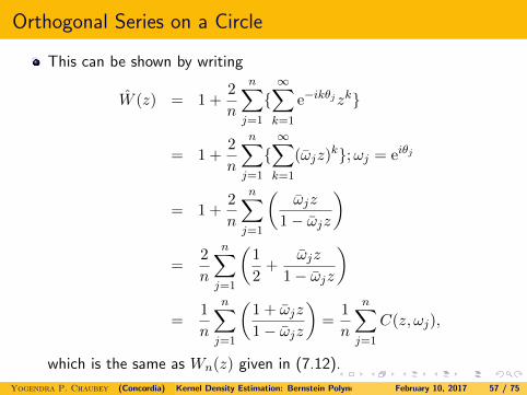
Orthogonal Series on a Circle

This can be shown by writing

W (z) = 1 +2

n

n∑j=1

{∞∑k=1

e−ikθjzk}

= 1 +2

n

n∑j=1

{∞∑k=1

(ωjz)k};ωj = eiθj

= 1 +2

n

n∑j=1

(ωjz

1− ωjz

)

=2

n

n∑j=1

(1

2+

ωjz

1− ωjz

)

=1

n

n∑j=1

(1 + ωjz

1− ωjz

)=

1

n

n∑j=1

C(z, ωj),

which is the same as Wn(z) given in (7.12).


6.2 Orthogonal Series on a Circle

Remark:

This ensures that the orthogonal series estimator of the densitycoincides with the circular kernel estimator.

The determination of the smoothing constant may be handled basedon the cross validation method outlined in [20]

Note that the simplification used in the above formulae does not workfor r = 1. Even though, the limiting form of (7.15) is used to definean orthogonal series estimator as given by

fS(θ) =1

2π+

1

πn

n∑j=1

n∗∑k=1

cos k(θ − θj), (7.16)

where n∗ is chosen according to some criterion, for example tominimize the integrated squared error.


Orthogonal Series on a Circle

Thus the above discussion presents two contrasting situations: in onewe have to determine the number of terms in the series and in theother number of terms in the series is allowed to be infinite, however,we choose to evaluate Re W (eiθ) for some r close to 1 as anapproximation to Re W (eiθ).

Considering above discussions, we provide below some examples usingthe von Mises and wrapped Cauchy kernels and contrast them withusing the inverse stereographic kernels using the normal and logisticdistributions.

It is seen that wrapped Cauchy may provide estimators that are notas smooth as those provided by other methods. Further investigationof these methods is in progress.


Turtle Data

The following Table gives the measurements of the directions taken by76 turtles after treatment from Appendix B.3 in Fisher (1993). Thisdata has been analysed in Fisher (1989) and Prakasa Rao (1986.)8,38,50,64,83,98,204,257, 9,38,53,65,88,100,215,268,13,40,56,65,88,103,223,285, 13,44,57,68,88,106,226,319,14,45,58,70,90,113,237,343, 18,47,58,73,92,118,238,350,22,48,61,78,92,138,243, 27,48,63,78,93,153,244,30,48,64,78,95,153,250, 34,48,64,83,96,155,251


Turtle Data - WC Kernel:

Histogram and Circular Kernel Density

Turtle Data, Stefens(1969)Theta

Dens

ity

0 1 2 3 4 5 6 7

0.00.1

0.20.3

0.4 Rho=.6Rho=.7Rho=.8

Figure: 1. Histogram and Circular Kernel Density with wrapped Cauchy;ρ = .6, .7, .8.


Turtle Data - VM Kernel:

Histogram and Circular Kernel VM Density

Turtle Data, Stefens(1969)Theta

Dens

ity

0 1 2 3 4 5 6 7

0.00.1

0.20.3

0.4 Kappa=3Kappa=4Kappa=5

Figure: 2. Histogram and Circular Kernel Density with von Mises; κ = 3, 4, 5.


Turtle Data - ISC Normal Kernel:

Histogram and Circular Kernel ISCNorm Density

Turtle DataTheta

Dens

ity

0 1 2 3 4 5 6 7

0.00.1

0.20.3

0.4 sigma=.25sigma=.3sigma=.35

Figure: 3. Histogram and Circular Kernel Density with ISCNorm Kernel;σ = .25, .3, .35.


Turtle Data - ISC Logistic Kernel:

Histogram and Circular Kernel ISCLogistic Density

Turtle DataTheta

Dens

ity

0 1 2 3 4 5 6 7

0.00.1

0.20.3

0.4 sigma=.15sigma=.25sigma=.35

Figure: 4. Histogram and Circular Kernel Density with ISCLogistic Kernel;σ = .15, .25, .35.


Turtle Data

The following Table gives the measurements of the directions chosenby 100 ants in response to an evenly illuminated black target fromAppendix B.7 in Fisher (1993).330,180,160,200,180,190,10,160,110,140,290,160,200,180,160,210,220,180,270,40,60,280,190,120,210,220,180,120,180,300,200,180,250,200,190,200,210,150,200,80,200,170,180,210,180,60,170,300,180,210,180,190,30,130,230,260,90,190,140,200,280,180,200,30,50,110,160,220,360,170,220,140,180,210,150,180,180,160,150,200,190,150,200,200,210,220,170,70,160,210,180,150,350,230,180,170,200,190,170,190


Ants Data - WC Kernel:

Histogram and Circular Kernel WC Density

Ants DataTheta

Dens

ity

0 1 2 3 4 5 6 7

0.00.1

0.20.3

0.40.5 Rho=.81

Rho=.82Rho=.83

Figure: 5. Histogram and Circular Kernel Density with wrapped Cauchy;ρ = .81, .84, .86.


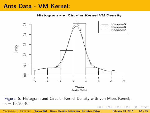
Ants Data - VM Kernel:

Histogram and Circular Kernel VM Density

Ants DataTheta

Dens

ity

0 1 2 3 4 5 6 7

0.00.1

0.20.3

0.40.5 Kappa=5

Kappa=6Kappa=7

Figure: 6. Histogram and Circular Kernel Density with von Mises Kernel;κ = 10, 20, 40.


Ants Data - ISC Normal Kernel:

Histogram and Circular Kernel ISCNorm Density

Ants DataTheta

Dens

ity

0 1 2 3 4 5 6 7

0.00.1

0.20.3

0.40.5 sigma=.2

sigma=.25sigma=.3

Figure: 7. Histogram and Circular Kernel Density with ISCNorm kernel;σ = .2, .25, .3.


Turtle Data - ISC Logistic Kernel:

Histogram and Circular Kernel ISCLogistic Density

Ants DataTheta

Dens

ity

0 1 2 3 4 5 6 7

0.00.1

0.20.3

0.40.5 sigma=.15

sigma=.25sigma=.35

Figure: 8. Histogram and Circular Kernel Density with ISCNorm kernel;σ = .15, .25, .35.


Conclusion:

The von Mises kernel seems to provide smoother plots as compared to WCbut they are qualitatively similar. The estimators obtained by IStransformation also produce similar results as to those given by the circularkernel estimators. Smoothing parameter may be selected using theproposal described in Taylor (2008). An enhanced strategy is toinvestigate a range of values around the value given by cross-validation.


References1 Abe, T. and Pewsey, A. (2011). Symmetric Circular Models Through

Duplication and Cosine Perturbation. Computational Statistics &Data Analysis, 55(12), 3271–3282.

2 Babu, G. J.; Canty, A.; Chaubey, Y. (2002). Application of Bernsteinpolynomials for smooth estimation of a distribution and densityfunction. J. Statist. Plann. Inference , 105, 377-392.

3 Babu, G. Jogesh, and Chaubey, Yogendra P. (2006). Smoothestimation of a distribution and density function on hypercube usingBernstein polynomials for dependent random vectors. Statistics andProbability Letters, 76, 959-969.

4 Bernstein, S. N. (1912). Demonstration du Theorme de Weierstrassfondee sur le calcul des Probabilites. Comm. Soc. Math. Kharkov 2Series XIII No.1, 1-2.

5 Carnicero, J.A., Wiper, M.P. and Ausın, M.C. (2010). CircularBernstein polynomial distributions. Working Paper 10-25, Statisticsand Econometrics Series 11, Departamento de Estadstica UniversidadCarlos III de Madrid. e-archivo.uc3m.es/bitstream/handle/

10016/8318/ws102511.pdf?sequence=1


e-archivo.uc3m.es/bitstream/handle/10016/8318/ws102511.pdf?sequence=1

e-archivo.uc3m.es/bitstream/handle/10016/8318/ws102511.pdf?sequence=1

References6 Chaubey, Yogendra P. (2016). Smooth Kernel Estimation of a

Circular Density Function: A Connection to Orthogonal Polynomialson the Unit Circle. Preprint, https://arxiv.org/abs/1601.05053

7 Chaubey, Yogendra P.; Li, J.; Sen, A. and Sen, P.K. (2012). A newsmooth density estimator for non-negative random variables. Journalof the Indian Statistical Association, 50, 83-104.

8 Di Marzio, M., Panzera, A., Taylor, C.C. (2009). Local PolynomialRegression for Circular Predictors. Statistics & Probability Letters,79(19), 2066–2075.

9 Feller, W. (1966). An Introduction to Probability Theory and itsApplications, Vol. II. New York: Wiley.

10 Fisher, N.I. (1989). Smoothing a sample of circular data, J.Structural Geology, 11, 775–778.

11 Fisher, N.I. (1993). Statistical Analysis of Circular Data. CambridgeUniversity Press, Cambridge.


https://arxiv.org/abs/1601.05053

References

12 Mhaskar, H.N. and Pai, D.V. (2000). Fundamentals of approximationTheory. Narosa Publishing House, New Delhi, India.

13 Parzen, E. (1962). On Estimation of a Probability Density Functionand Mode. Ann. Math. Statist, 33:3, 1065-1076.

14 Petrone, S. and Veronese, P. (2010). Feller Operators and MixturePriors in Bayesian Nonparametrics. Statistica Sinica 20, 379-404

15 Prakasa Rao, B.L.S. (1983). Non Parametric Functional Estimation.Academic Press, Orlando, Florida.

16 Rudin, W. (1987). Real and Complex Analysis- Third Edition.McGraw Hill: New York.

17 Rosenblatt, M. (1956). Remarks on some nonparametric estimates ofa density function. Ann. Math. Stat., 27:56, 832837


References

18 Simon, B. (2005). Orthogonal Polynomials on the Unit Circle, Part 1:Classical Theory. American Mathematical Society, Providence, RhodeIsland.

19 Silverman B. W. (1986). Density Estimation for Statistics and DataAnalysis. London: Chapman & Hall.

20 Taylor, C.C. (2008). Automatic Bandwidth Selection for CircularDensity Estimation. Computational Statistics & Data Analysis, 52(7),3493–3500.

21 Vitale, R.A. (1973). A Bernstein polynomial approach to densityestimation. Commun Stat, 2, 493-506.

22 Weierstrass, K. (1885). Uber die analytische Darstellbarkeitsogenannter willkrlicher Functionen einer reellen Vernderlichen.Sitzungsberichte der Akademie zu Berlin 633-639 and 789-805.


And the story continues....Thanks!

Talk slides will be available onSlideShare:http://www.slideshare.net/ychaubey/talk-slides-imsct2016-70230405www.slideshare.net/ychaubey/talk-slides-imsct2016-70230405

THANKS!!


www.slideshare.net/ychaubey/talk-slides-imsct2016-70230405

chaubey seminarslides2017

Education