characterization of sae 52100 bearing steel for …etd.lib.metu.edu.tr/upload/12617985/index.pdf ·...

CHARACTERIZATION OF SAE 52100 BEARING STEEL FOR

FINITE ELEMENT SIMULATION OF THROUGH-HARDENING PROCESS

A THESIS SUBMITTED TO

THE GRADUATE SCHOOL OF NATURAL AND APPLIED SCIENCES

OF

MIDDLE EAST TECHNICAL UNIVERSITY

BY

OZAN MÜŞTAK

IN PARTIAL FULFILLMENT OF THE REQUIREMENTS

FOR

THE DEGREE OF MASTER OF SCIENCE

IN

METALLURGICAL AND MATERIALS ENGINEERING

SEPTEMBER 2014

Approval of the thesis:


THROUGH HARDENING FINITE ELEMENT SIMULATION

submitted by OZAN MÜŞTAK in partial fulfillment of the requirements for the

degree of Master of Science in Metallurgical and Materials Engineering

Department, Middle East Technical University by,

Prof. Dr. Canan ÖZGEN _________

Dean, Graduate School of Natural and Applied Sciences

Prof. Dr. C. Hakan GÜR _________

Head of Department, Metallurgical and Materials Engineering

Prof. Dr. C. Hakan GÜR _________

Supervisor, Metallurgical and Materials Engineering Dept., METU

Asst. Prof. Dr. Caner ŞİMŞİR _________

Co-Supervisor, Manufacturing Engineering Dept., Atılım University

Examining Committee Members:

Prof. Dr. Rıza GÜRBÜZ _____________________

Metallurgical and Materials Eng. Dept., METU

Prof. Dr. C. Hakan GÜR _____________________


Prof. Dr. Bilgehan ÖGEL _____________________


Asst. Prof. Dr. Eren KALAY _____________________


Dr.-Ing Feridun ÖZHAN _____________________

Technical General Manager, ORS BEARINGS INC.

Date: 09.09.2014

iv

I hereby declare that all information in this document has been obtained and

presented in accordance with academic rules and ethical conduct. I also declare

that, as required by these rules and conduct, I have fully cited and referenced

all material and results that are not original to this work.

Name, Last name : Ozan MÜŞTAK

Signature :

v

ABSTRACT


FINITE ELEMENT SIMULATION OF THROUGH-HARDENING PROCESS

Müştak, Ozan

M.S., Department of Metallurgical and Materials Engineering

Supervisor : Prof. Dr. C. Hakan Gür

Co-Supervisor : Asst. Prof. Dr. Caner Şimşir

September 2014, 116 pages

Through hardening is probably the most important heat treatment process for

bearings as final geometrical and material characteristics of the final component are

mainly determined in this step. Finite element simulation of heat treatment processes

is stand out as a qualified solution for prediction of final properties of component

due to advantages e.g. cost and time savings, over real-time furnace experiments.

Heat treatment simulation needs accurately extracted material property database

including thermo-physical and thermo-mechanical properties of the all phases as a

function of temperature. However, only a fraction of these data are available for

100Cr6 (SAE 52100). The present study aimed to the determination of thermo-

mechanical and thermo-metallurgical properties of 100Cr6 bearing steel, which are

necessary for through hardening simulation, by using a combination of experimental

and computational methods. Briefly, the study includes experimental determination

of temperature dependent physical properties (e.g. thermal expansion coefficient),

temperature dependent mechanical properties (e.g. flow curves, yield strengths,

transformation strains, thermal strains), phase transformation kinetics, (e.g.

TTT/CCT diagrams), critical temperatures (Ms, Mf, Bs, Ac1 and Ac3) and

vi

investigating the effect of stress on phase transformation. Thermal conductivity, heat

capacity, elastic modulus, Poisson’s ratio, enthalpy and density values were

calculated using physically based computational methods.

Keywords: Material Characterization, Dilatometry, Finite Element Simulation,

Through Hardening.

vii

ÖZ

SERTLEŞTİRME ISIL İŞLEMİNİN SONLU ELEMANLAR YÖNTEMİ İLE

BENZETİMİ İÇİN SAE 52100 RULMAN ÇELİĞİNİN

KARAKTERİZASYONU

Müştak, Ozan

Yüksek Lisans, Metalurji ve Malzeme Mühendisliği Bölümü

Tez Yöneticisi : Prof. Dr. C. Hakan Gür

Ortak Tez Yöneticisi : Yrd. Doç. Dr. Caner Şimşir

Eylül 2014, 116 sayfa

Sertleştirme, rulman bileziklerinin nihai geometrilerinin ve malzeme

karakteristiklerinin belirlendiği başlıca üretim basamaklardan biri olması açısından

belki de en önemli ısıl işlem prosesidir. Isıl işlem için sonlu elemanlar benzetimi,

bileşenin ısıl işlem sonrası özelliklerinin tahmin edilmesi istendiğinde fırınlarda

yapılacak gerçek zamanlı deneylere göre maliyet ve zaman tasarrufu sağlaması

açısından ön plana çıkmaktadır. Isıl işlem benzetimi, tüm fazların sıcaklığa bağlı

olarak termo-fiziksel ve termo-mekanik özelliklerini içeren hassas bir şekilde

oluşturulmuş malzeme veri setine ihtiyaç duymaktadır. Bununla birlikte, bu verilerin

sadece bir kısmı 100Cr6 (SAE 52100) için kullanılabilir durumdadır. Bu çalışmada,

sertleştirme ısıl işlemi benzetimi için gerekli olan, 100Cr6 rulman çeliğinin termo-

mekanik ve termo-metalurjik özelliklerinin, deneysel ve hesaplamalı yöntemler

kullanılarak oluşturulması amaçlanmıştır. Deneysel yöntemler kullanılarak; sıcaklığa

bağlı olarak fiziksel özellikler; termal genleşme katsayısı belirlenmiş, sıcaklığa bağlı

olarak mekanik özellikler; kuvvet-akma eğrileri, dönüşüm gerinmesi, termal

gerinmeler, faz dönüşüm kinetiği; TTT/CCT diyagramları, kritik sıcaklıklar (Ms,

viii

Mf, Bs, Ac1, Ac3) hesaplanmış ve gerilimin faz dönüşümüne etkisi incelenmiştir.

Termal iletkenlik, ısı sığası, elastik modülü, Poisson katsayısı, entalpi ve yoğunluk

gibi değerler fiziksel tabanlı hesaplamalı yöntemler kullanılarak hesaplanmıştır.

Anahtar Kelimeler: Malzeme Karakterizasyonu, Dilatometri, Sonlu Elemanlar

Simülasyonu, Sertleştirme Isıl İşlemi.

ix

To My Family…

xi

ACKNOWLEDGEMENTS

The author would like to express sincere gratitude to his supervisor, Prof. Dr. C.

Hakan GÜR for giving opportunity to work with him on this research, and also thank

for his encouragement, guidance, and support during the research.

The author would like to express his deepest and special appreciation to his co-

supervisor Asst. Prof. Dr. Caner ŞİMŞİR. This work would not be possible without

his encouragement, knowledge, guidance, patience, help, and support throughout the

research.

The author would like to express gratitude to his managers, Dr.-Ing Feridun

ÖZHAN, Turhan SAVAŞ and Dr.-Ing Hamdullah MERDANE at ORS Bearings Inc.

for their encouragement, guidance and support. The author also would like to express

his gratitude to his colleagues, Halil Onat TUĞRUL, Nazmi SAYDEMİR, Mustafa

HORTAÇ, Nedim Özgür ENGİN and Zeren TAŞKAYA on behalf of all ORS

Bearings Inc. members, for their encourage, interest, help, support and technical

assistance.

The author would like to express his thank to Dr. Kemal DAVUT, Tuba

DEMİRTAŞ, Deniz DURAN, Nezih MUMCU, Elif EVCİL and all other members

of Metal Forming Center of Excellence for their valuable technical assistance, help

and support during this research.

The author owes his deepest gratitude to his parents, Nazmiye MÜŞTAK, Mehmet

MÜŞTAK and his brother Hamit Kaan MÜŞTAK for their gentle love, inspiration,

support and guidance throughout his life.

The author would like to thank heartily to Gül YÜCEL for her love, friendship and

support since they met in 2008.

xii

Special thanks go to Ümit AKÇAOĞLU, Murat KAMBEROĞLU, Onur DEMİREL,

Erdem MERMER, Sadık YETKİN, Emre AKBAŞ and Murat ÇETİNKIRAN for

their friendship, help and support.

This research was financially supported by a SANTEZ project. The author would

like to acknowledge Ministry of Science, Industry and Technology of Republic of

Turkey and ORS Bearings Inc. for their financial support.

The author would like to acknowledge ONATUS Company for their permission to

use of SYSWELD® software in this thesis.

Finally, the author would like to offer his regards and blessings to all of those who

supported him in any respect during this research.

xiii

TABLE OF CONTENTS

ABSTRACT ................................................................................................................. v

ÖZ .............................................................................................................................. vii

ACKNOWLEDGEMENTS ........................................................................................ xi

TABLE OF CONTENTS ......................................................................................... xiii

LIST OF TABLES ................................................................................................... xvii

LIST OF FIGURES ............................................................................................... xviii

LIST OF SYMBOLS AND ABBREVIATIONS .................................................... xxv

CHAPTERS

1. INTRODUCTION ................................................................................................ 1

2. THEORY AND LITERATURE SURVEY .......................................................... 7

2.1. Quenching ........................................................................................................... 7

2.2. Heat Treatment Simulation and Simulation of Quenching ................................ 9

2.3. Phase Transformations in Steels ....................................................................... 10

2.3.1. Diffusional Phase Transformations ........................................................... 10

2.3.2. Displacive Phase Transformations ............................................................ 10

2.4. Kinetics of Phase Transformations ................................................................... 11

2.4.1. Kinetics of Diffusional Phase Transformations ........................................ 11

2.4.2. Kinetics of Displacive Phase Transformations .......................................... 13

2.5. Effect of Stress on Phase Transformations and Transformation Plasticity ...... 14

2.6. Thermo-physical Properties .............................................................................. 16

2.6.1. Coefficient of Thermal Expansion, Thermal and Transformation Strains 16

2.6.2. Density ....................................................................................................... 17

2.6.3. Thermal Conductivity, Specific Heat Capacity and Enthalpy ................... 19

2.7. Mechanical Properties ...................................................................................... 19

xiv

2.7.1. Material Models for Mechanical Interactions ........................................... 19

2.7.2. Strain Constituents .................................................................................... 20

2.8. Experimental Determination of Material Properties by Dilatometry ............... 21

2.8.1. Alpha and Sub-Zero Dilatometry .............................................................. 22

2.8.2. Quenching Dilatometry ............................................................................. 22

2.8.3. Deformation Dilatometry .......................................................................... 23

2.8.4. Stressed Dilatometry ................................................................................. 23

3. EXPERIMENTAL DETERMINATION OF MATERIAL PROPERTIES ....... 25

3.1. Experimental Setup and Procedure .................................................................. 25

3.1.1. Dilatometer ................................................................................................ 25

Dilatometer Samples ............................................................................. 27

Preparation of Dilatometer Samples ..................................................... 28

Temperature Programs used in Dilatometry Experiments ................... 29

Temperature Programs used for CCT Tests..................................... 30

Temperature Programs used for TTT Tests ..................................... 32

Temperature Programs for Mechanical Tests of Austenite ............. 33

Temperature Programs for Mechanical Tests of Martensite and

Bainite 35

Temperature Programs used in TRIP Tests for Bainitic

Transformation ................................................................................................. 36

Temperature Program used in TRIP Tests for Martensitic

Transformation ................................................................................................. 37

Temperature Programs used for Sub-Zero Tests ............................. 39

3.1.2. XRD........................................................................................................... 39

3.1.3. SEM ........................................................................................................... 40

3.2. Evaluation Procedures and Results .................................................................. 41

xv

3.2.1. Evaluation of a Dilatometric Curve ........................................................... 41

3.2.2. Determination of Time-Temperature-Transformation (TTT) Diagram .... 42

Evaluation Procedure of TTT Tests ...................................................... 43

Results of TTT Tests ............................................................................. 45

3.2.3. Determination of Continuous Cooling Transformation (CCT) Diagram .. 49

Evaluation Procedure of CCT Tests ..................................................... 49

Results of CCT Tests ............................................................................ 50

3.2.4. Determination of Critical Temperatures (Ms, Mf, Bs, Ac1 and Ac3) ....... 55

Evaluation and Calculation Procedure for Critical Temperatures ........ 55

Results of Calculations for Critical Temperatures ................................ 56

3.2.5. Determination of Thermal Expansion Coefficient .................................... 58

Evaluation Procedure for Thermal Expansion Coefficient ................... 59

Results for Calculations of Thermal Expansion Coefficient ................ 60

3.2.6. Determination of Densities for Spheroidite, Austenite and Martensite..... 60

Evaluation Procedure for Densities of Phases ...................................... 61

Results of Density Calculations ............................................................ 62

3.2.7. Determination of Thermal and Transformation Strains ............................ 63

Evaluation Procedure for Thermal and Transformation Strains ........... 63

Results of Calculations for Thermal and Transformation Strains ........ 64

3.2.8. Determination of Mechanical Properties of Austenite, Martensite and

Bainite Phases ........................................................................................................ 65

Evaluation Procedure for Mechanical Tests ......................................... 66

Results of Mechanical Tests ................................................................. 67

3.2.9. Determination of the Effect of Stress on Phase Transformations ............. 73

Evaluation Procedure for TRIP Tests ................................................... 73

Results of TRIP Tests ........................................................................... 75

xvi

4. COMPUTATIONAL DETERMINATION OF MATERIAL PROPERTIES.... 79

4.1. General ............................................................................................................. 79

4.2. Theory............................................................................................................... 79

4.2.1. Calculation of TTT and CCT diagrams ..................................................... 82

4.3. Calculation and Evaluation Procedure ............................................................. 82

4.4. Results .............................................................................................................. 83

5. JUSTIFICATION AND EVALUATION OF MATERIAL DATA SET ........... 91

5.1. Implementation of the Material Data Set into SYSWELD® ........................... 91

5.1.1. Implementation of Thermo-Physical Properties ........................................ 91

5.1.2. Implementation of Thermo-Metallurgical Properties ................................ 92

5.1.3. Implementation of Thermo-Mechanical Properties .................................. 92

5.2. Through-Hardening Simulation for Conical Bearing Ring .............................. 93

5.2.1. Details of Simulation ................................................................................. 94

5.2.2. Results ....................................................................................................... 95

Cooling Curves ..................................................................................... 95

Phase Proportions ................................................................................. 97

Dimensional Changes ........................................................................... 99

Evolution of Stresses during Quenching ............................................ 100

6. CONCLUSION AND OUTLOOK ................................................................... 107

REFERENCES ........................................................................................................ 111

xvii

LIST OF TABLES

TABLES

Table 1: Standard chemical composition of SAE 52100. ............................................ 1

Table 2: Chemical Composition of 100Cr6 used in the study. Composition was given

as Wt. (%)................................................................................................................... 28

Table 3: Details of dilatometer temperature programs used in tests. ......................... 30

Table 4: List of specimens used in CCT tests with t8/5 times. .................................... 31

Table 5: List of specimens used in TTT tests. ........................................................... 33

Table 6: Parameters used in temperature programs of mechanical tests of meta-stable

austenite...................................................................................................................... 34

Table 7: Parameters used in temperature program of mechanical tests of bainite. .... 35

Table 8: Parameters used in temperature program of mechanical tests of martensite.

.................................................................................................................................... 35

Table 9: Loads applied on specimens at TRIP tests of bainitic phase transformation.

.................................................................................................................................... 37

Table 10: Loads applied on specimens at TRIP tests of martensite phase................. 38

Table 11: Number of experiments evaluated in this study. ........................................ 41

Table 12: Thermal Strains calculated at 0 °C and 1000 °C. ...................................... 65

Table 13: Transformation Strains calculated at 20 °C and 850 °C. ........................... 65

Table 14: Results for calculations of transformation plasticity constants of bainitic

and martensitic phases at 350 °C. .............................................................................. 78

Table 15: Compositions used for computational part of the study. ........................... 84

Table 16: Summary for calculated and determined Thermo-Physical Properties. ..... 89

Table 17: Summary for calculated and determined Thermo-Mechanical Properties. 89

Table 18: Summary for calculated and determined Thermo-Metallurgical Properties.

.................................................................................................................................... 90

xviii

LIST OF FIGURES

FIGURES

Figure 1: Physical fields and couplings during quenching. ......................................... 8

Figure 2: Representative S-shape curve for an isothermal transformation. ............... 12

Figure 3: Schematic representation of Scheil’s additivity principle. ......................... 13

Figure 4: Relative change in length vs. temperature of 100Cr6 with an initial

spheroidite microstructure showing complete transformation of initial phase to

austenite. Temperature interval of 720-860 °C was plotted. ..................................... 21

Figure 5: (a) Chamber of Baehr-Thermoanalysis GmbH, DIL 805 A/D dilatometer

and (b) induction coil used in DIL 805 A/D. ............................................................. 25

Figure 6: Schematic representation of DIL 805 A/D in quenching mode. ①

Pt90Rh10–Pt (S-Type) thermocouple, ② LVDT, ③ Induction Coil, ④ Push rods, ⑤

Separation wall and ⑥ Specimen. ............................................................................. 26

Figure 7: Dilatometer specimens; Ø5x10mm specimen for mechanical tests of

bainite and austenite (a), Ø4x8mm specimen for mechanical tests of martensite (b),

Ø4x10mm, bore diameter of Ø2mm specimen for CCT and TTT tests (c),

Ø4x10mm, bore diameter of Ø3.96mm specimen for sub-zero tests (d). .................. 28

Figure 8: Position of the specimens extracted from sliced rod. ................................. 29

Figure 9: Representative Temperature Program for CCT Tests. ............................... 32

Figure 10: Representative temperature program for TTT tests. ................................ 33

Figure 11: Representative temperature program for mechanical tests of meta-stable

austenite. .................................................................................................................... 34

Figure 12: Representative temperature program for mechanical test of bainitic and

martensitic phases. ..................................................................................................... 36

Figure 13: Representative temperature program for TRIP tests of bainitic phase

transformation. ........................................................................................................... 37

Figure 14: Representative temperature program for TRIP test of martensite phase.. 38

Figure 15: Representative temperature program for sub-zero tests. .......................... 39

xix

Figure 16: X-Ray Diffractometer (XRD), Seifert 3003 PTS. (a) X-Ray Generator

Tube, (b) 5-Axis Goniometer and (c) Position Sensitive Detector (PSD). ................ 40

Figure 17: Relative change in length vs. temperature plot. “A-B” is heating segment,

“B-C” is spheroidite to austenite phase transformation, “C-D” refers to thermal

expansion of push rods, “D-E” is the cooling segment. ............................................. 42

Figure 18: Relative change in length vs. time plot. Point “A” refers to %1 of

transformation and point “B” refers to %99 of transformation.................................. 44

Figure 19: JMA fitted, % Phase transformed vs. time plot of some experiments...... 45

Figure 20: TTT Diagram of Steel 100Cr6. Austenitized at 850 °C for 30 minutes.

Computed TTT Diagram with JMatPro and TTT Diagram given in Atlas [65]

(Austenitization 860°C – 15 min.) also plotted for comparison. ............................... 46

Figure 21: SEM Images of TTT specimens after experiments performed at various

temperatures, x15000 magnification, and pearlitic microstructure with spheroidized

carbides (bright). ........................................................................................................ 47


temperatures, x15000 magnification, and bainitic microstructure with spheroidized

carbides (bright). ........................................................................................................ 48

Figure 23: Relative change in length vs. temperature plot for CCT test No6-026.

Point “A” represents beginning of austenite to bainite transformation, point "B"

represents completion of austenite to bainite transformation and point "C"

commented as the beginning of austenite to martensite transformation. ................... 50

Figure 24: CCT diagram of steel 100Cr6. Diagram computed via JMatPro® and

diagram found in Atlas [65] (Austenitization 860°C – 15 min.) also plotted for

comparison. Cooling curves and hardness values are also indicated. ........................ 51

Figure 25: SEM Image of test No1 with t8/5: 14 s. 10K X magnification. Martensitic

microstructure with some spheroidized carbides (bright). ......................................... 52

Figure 26: SEM Image of test No2 with t8/5: 16 s. 10K X magnification. Martensitic

and bainitic microstructure with spheroidized carbides (bright). .............................. 52

Figure 27: SEM Image of set No3 with t8/5: 20 s. 10K X magnification. Martensitic

and bainitic microstructure. ........................................................................................ 53

xx

Figure 28: SEM Image set No3.4 with t8/5: 23 s. 10K X magnification. Martensitic

and bainitic microstructure. ....................................................................................... 53

Figure 29: SEM Image of set No3.7 with t8/5: 27 s. 10K X magnification. Martensitic


Figure 30: SEM Image set No4 with t8/5: 30 s. 10K X magnification. Martensitic and

bainitic microstructure. .............................................................................................. 53

Figure 31: SEM Image of set No4.4 with t8/5: 36 s. 10K X magnification. Martensitic


Figure 32: SEM Image of set No4.7 with t8/5: 40 s. 10K X magnification. Pearlitic


Figure 33: SEM Image of set No5 with t8/5: 44 s. 10K X magnification. Pearlitic and

bainitic microstructure. .............................................................................................. 54

Figure 34: SEM Image of set No6 with t8/5: 50.4 s. 10K X magnification. Pearlitic


Figure 35: SEM Image of experiment from set No7 with t8/5: 62.8 s. 10K X

magnification. Pearlitic microstructure with spheroidized carbides (bright). ............ 54

Figure 36: SEM Image of experiment from set No8 with t8/5: 87 s. 10K X




Figure 38: Sub-zero experiment No111 interval of (-)130 °C – (+)300 °C. .............. 57

Figure 39: Phase transformed [%] vs temperature [°C] plot of sub-zero test and

kinetic model fittings of Koistinen-Marburger and modified Koistinen-Marburger. 58

Figure 40: Relative change in length [%] vs. temperature [°C] representative plot for

CCT tests. Slope of “A” refers to thermal expansion coefficient of spheroidite. Slope

of “B” refers to thermal expansion coefficient of austenite. ...................................... 59

Figure 41: Densities of Spheroidite, Austenite and Martensite with respect to

temperature. JMatPro® and literature [12, 13] values for densities are also shown. 63

Figure 42: Thermal strains of martensite, spheroidite and austenite phases for steel

100Cr6. Transformation strains 𝜀𝐴 → 𝑀 𝑡𝑟, 𝜀𝑆 → 𝐴𝑡𝑟 and 𝜀𝑆 → 𝑀𝑡𝑟 also indicated

on the figure. .............................................................................................................. 64

xxi

Figure 43: Ramberg-Osgood Model fitting for mechanical test of austenite at 850°C.

.................................................................................................................................... 67

Figure 44: Results of calculations for mechanical tests of austenite and regression

line fitted for material parameter 𝐾𝑅𝑂 w.r.t. temperature. ........................................ 69

Figure 45: Temperature dependency of hardening exponent 𝑛𝑅𝑂 and regression line

fitted onto calculated values of mechanical tests of austenite.................................... 69

Figure 46: Results of calculations for mechanical tests of bainite and regression line

fitted for material parameter 𝐾𝑅𝑂 w.r.t. temperature. ............................................... 69


fitted onto calculated values of mechanical tests of bainite. ...................................... 69

Figure 48: Results of calculations for mechanical tests of martensite and regression

line fitted for material parameter 𝐾𝑅𝑂 w.r.t. temperature. ........................................ 69


fitted onto calculated values of mechanical tests of martensite. ................................ 69

Figure 50: True stress vs. true plastic strain plots for meta-stable austenite for a

temperature range 300°C-850°C. Flow curves from the literature [12] are also

indicated. .................................................................................................................... 70

Figure 51: True stress vs. true plastic strain plots for bainitic phase for a temperature

range 100°C-600°C. ................................................................................................... 71

Figure 52: True stress vs. true plastic strain plots for martensitic phase for a

temperature range 100°C-450°C. Flow curves found in literature [12] are also

indicated. .................................................................................................................... 71

Figure 53: Yield strengths of meta-stable austenite as a function of temperature.

Yield strengths found in literature and computed via JMatPro® are also indicated. 72

Figure 54: Yield strength of bainitic phase with respect to temperature. .................. 73

Figure 55: Yield strength of martensitic phase as a function of temperature. ........... 73

Figure 56: The effect of stress on bainitic phase transformation. .............................. 74

Figure 57: Modified Koistinen-Marburger fitted dilatometric curves of TRIP tests of

martensitic transformation. Extrapolated regions are indicated as dashed lines. ....... 75

Figure 58: Transformation plasticity strain vs. applied load plot for bainitic phase

transformation. ........................................................................................................... 76

xxii

Figure 59: Transformation plasticity strain vs. applied load plot for martensitic phase

transformation. ........................................................................................................... 76

Figure 60: Theoretically calculated transformation plasticity parameter vs.

temperature plot for martensitic phase transformation. ............................................. 78

Figure 61: Calculation procedure for material property and methods used for each

calculation step........................................................................................................... 80

Figure 62: Comparison of phase amounts between diminutive differences in

chemical composition of steel 100Cr6. “Composition 1” is the composition used in

this study and “Composition 2” is standard composition for 100Cr6. ...................... 84

Figure 63: Comparison of density values computed (solid) and found in the literature

(dashed) for martensitic and austenitic phases as a function of temperature. ............ 85

Figure 64: Specific heat for each phase of 100Cr6 with respect to temperature. ...... 86

Figure 65: Thermal conductivity for each phase of 100Cr6 with respect to

temperature. ............................................................................................................... 86

Figure 66: Enthalpy for each phase of 100Cr6 with respect to temperature. ............ 87

Figure 67: Young's modulus for each phase of 100Cr6 with respect to temperature.87

Figure 68: Poisson’s ratio for each phase of 100Cr6 with respect to temperature. ... 88

Figure 69: Conical bearing ring used in through-hardening simulation. ................... 93

Figure 70: The mesh used in simulations. Boundary conditions (arrows) and

important nodes (+) are also indicated. #1 bottom side, #2 core, #3 inner side, #4

outer side, #5 group of nodes represented as line and #6 top side. ............................ 95

Figure 71: Comparison of cooling curves obtained from simulations with literature.

.................................................................................................................................... 96

Figure 72: Detailed view of cooling curves given in Figure 71. ............................... 96

Figure 73: Phase fraction of martensite during quenching. Comparison of martensitic

transformations results with the literature.................................................................. 98

Figure 74: Detailed view of the red box indicated in the Figure 73. ......................... 98

Figure 75: Changes in outer radius of conical bearing ring. ...................................... 99

Figure 76: Changes in bottom face of the conical bearing ring. ................................ 99

xxiii

Figure 77: Representative tilting of the rings. Nominal shape (gray) and deformed

shapes for both literature (orange) and simulations performed (blue) are also given.

Measurement results found in the literature indicated as red line. ........................... 100

Figure 78: Final shape of conical ring for the literature data [13] (green). Shape of

the ring before the simulation is indicated as the red box. ....................................... 100

Figure 79: Final shape of conical ring for data set created for this study (green).

TRIP constant taken as 1.06x10-5 [MPa]. ................................................................ 100

Figure 80: Variation of axial and tangential components of internal stresses at core

and surface during quenching with temperature difference between core and surface

of the conical ring..................................................................................................... 101

Figure 81: Distribution of axial component of the internal stresses observed on the

conical ring at 7th seconds. ....................................................................................... 102

Figure 82: Distribution of tangential component of the internal stresses observed on

the conical ring at 7th seconds. ................................................................................. 102


and surface during quenching with fraction of martensite calculated at core and

surface of the conical ring. ....................................................................................... 103

Figure 84: Distribution of axial component of internal stresses observed on the

conical ring at 40th seconds. ..................................................................................... 103

Figure 85: Distribution of tangential component of internal stresses observed on the

conical ring at 40th seconds. ..................................................................................... 103

Figure 86: Von Mises Stresses calculated for conical ring at the core and surface.

Yield strength of austenite is also indicated. ............................................................ 104

Figure 87: Distribution of axial component of residual stresses observed on the

conical ring at 250th seconds. ................................................................................... 105

Figure 88: Distribution of tangential component of residual stresses observed on the

conical ring at 250th seconds. ................................................................................... 105

Figure 89: Variation of axial components of residual stresses along the cross-section

of conical ring for a group of nodes of #5 for both simulations and literature. ....... 106

xxiv

Figure 90: Variation of tangential components of residual stresses along the cross-

section of conical ring for a group of nodes of #5 for both simulations and literature.

.................................................................................................................................. 106

xxv

LIST OF SYMBOLS AND ABBREVIATIONS

Abbreviations

FEM Finite Element Method

FDM Finite Difference Method

BEM Boundary Element Method

FEA Finite Element Analysis

EDM Electrical Discharge Machining

SEM Scanning Electron Microscopy

TRIP Transformation Induced Plasticity

FCC Face Centered Cubic

BCC Body Centered Cubic

CCT Continuous Cooling Transformation

TTT Time-Temperature-Transformation

DCCT Continuous Cooling Transformation after Deformation

DTTT Time-Temperature-Transformation after Deformation

CTE Coefficient of Thermal Expansion

JMA Johnson-Mehl-Avrami

XRD X-Ray Diffractometer

PSD Position Sensitive Detector

GCL Guarded-Comparative-Longitudinal

DSC Differential Scanning Calorimetry

DTA Differential Thermal Analysis

LVDT Linear Variable Differential Transformer

RMS Root Mean Square

CALPHAD Computer Coupling of Phase Diagrams and Thermochemistry

HTC Heat Transfer Coefficient

xxvi

Roman Symbols

P Volume fraction

Pi Volume fraction of phase i

Pi Property of phase i

P0 Property of phase in pure element

Pmix Property of the mixture

P(T) Material property at a given temperature

Xi Mole fraction for phase i

P(t) Amount of new phase transformed in time t Johnson-Mehl-Avrami equation

n(T) Temperature dependent time exponent for Johnson-Mehl-Avrami equation

k(T) Temperature dependent isothermal rate constant for JMA equation

H Enthalpy

H0 Standard enthalpy

G0 Gibbs Free Energy of pure components

q Heat flux

q Exponent dependent on the effective diffusion mechanism

KRO Material parameter for Ramberg-Osgood equation

Ktp Transformation plasticity parameter

K Hardening constant

N ASTM grain size

D Effective diffusion coefficient

E Elastic modulus

𝑛𝑅𝑂 Strain hardening exponent for Ramberg-Osgood equation

n Hardening exponent

n Exponent for modified Koistinen Marburger equation

f(z) Progress of transformation plasticity function

ck Multiplier for equation used for calculation of TRIP strain

Ms Martensite start temperature

xxvii

Mf Martensite finish temperature

Bs Bainite start temperature

Ac1 Ac1 temperature

Ac3 Ac3 temperature

Cp Specific heat

T Temperature

Ti Initial temperature

Tf Final temperature

Tref Reference temperature

V Volume

Vi Initial volume

Vf Final volume

l Length

l0 Initial length

lf Final length

t Time

t8/5 Characteristic time

Greek Symbols

α Thermal expansion coefficient

True coefficient of thermal expansion

𝛼𝑣 Volumetric thermal expansion coefficient

𝛼𝑙 Linear thermal expansion coefficient

Ω Transformation rate constant in the Koistinen-Marburger equation

𝜀 Strain

𝜀𝑡𝑜𝑡 Total strain

𝜀𝑡𝑝 Transformation plasticity strain

𝜀𝑒𝑙 Elastic strain

xxviii

𝜀𝑝𝑙 Plastic strain

𝜀𝑡ℎ Thermal strain

𝜀𝑡𝑟 Transformation strain

𝜀𝑖→𝑗𝑡𝑟 Transformation strain of phase i to phase j transformation

𝜌 Density

𝜌𝑡𝑜𝑡 Total density

𝜌𝑖 Density of phase i

𝜅 Thermal conductivity

𝜑𝑣 Interaction parameter

𝜔𝑖𝑗𝑣 Binary interaction parameter between phase i and phase j

β Empirical coefficient for modified Kirkaldy model

𝜏 Shear stress

𝜏𝑚𝑎𝑥 Maximum shear stress

𝜎𝑡𝑟𝑢𝑒 True stress

𝜎𝑦 Yield strength

𝜎𝑦𝑖 Yield strength of phase i

Operators

∆𝑥 Change in x

∇𝑥 Gradient of x

• Scalar product

1

CHAPTER 1

INTRODUCTION

1. INTRODUCTION

Ball bearings are widely used in critical structural components utilized in assemblies

of industrial sectors such as automotive and transportation, machine tools, food,

chemical, energy, aircraft and aerospace. Main duty of ball bearings is to deliver the

motion with high speeds and carry remarkable loads with ease and high efficiency.

Generally, a ball bearing consists of four main parts which are inner and outer rings,

balls and a cage.

The material used for most of the bearing applications is SAE 52100 (DIN-EN

100Cr6, Material No: 1.3505) alloy steel, which has the basic alloying content such

as Cr (1.35–1.60 wt. %), Mn (0.25–0.45 wt. %) and Si (0.15–0.35 wt. %) [1] (Table

1). 100Cr6 is also known as the bearing steel, because it has good dimensional

stability, high machinability and high hardenability, which are the required

properties for most of the bearing applications [2].

Table 1: Standard chemical composition of SAE 52100.

Wt% C Si Mn P S Cr Mo Al Cu O

Min. 0.93 0.15 0.25 - - 1.35 - - - -

Max. 1.05 0.35 0.45 0.025 0.015 1.60 0.10 0.050 0.30 0.0015

In general, there are three methods used for manufacturing of bearing rings in the

industry. In the first method, steel rods are used as a raw material and the rods are

drilled and turned for giving the bearing ring shape. In the second method, as-

spheroidized seamless steel tubes are used as a raw material instead of rods, the

bearing ring form is given to the tubes by turning operations. In the third method,

steel rods are used as a raw material and in order to give a bearing ring shape, hot

2

forging operation is used as a first operation. After the production of inner and outer

rings with hot forging, final shape is given with spheroidization heat treatment, cold-

ring rolling, turning, through-hardening heat treatment and grinding processes

respectively.

The essential properties of bearing applications such as fatigue strength, wear

resistance, hardenability and dimensional stability, directly dependent on phases

involved and their distribution in the microstructure of the component. Final

microstructure and mechanical properties, except final residual stresses, are given by

through-hardening heat treatment to the bearing rings. Through residual stresses and

surface residual stresses are determined by tempering and grinding processes

respectively for the bearing rings. That is why, through-hardening is probably the

one of the most important process, among other manufacturing steps, for improving

mechanical properties of the bearing rings.

Final microstructure and the resultant physical properties can vary for through-

hardening process with changing parameters of heating rate, austenitization

temperature, isothermal dwell time, quenching rate and quench temperature [3]. In a

metallurgical point of view, final microstructure that is desired for bearing rings

consist of both martensite and some amount of retained austenite phases [4].

Determination of the optimum through-hardening process parameters is the key in

order to eliminate or minimize production losses and to get desired final geometrical

shape, mechanical properties and microstructure. This determination can be done via

experimental trials or numerical simulation methods. There are several software

codes and tools available, which are based on FEM, FDM and BEM, for simulation

of heat treatment process. Each experimental setup generally takes enormous amount

of time and can be very costly because trial & error approach with physical

experiments must be used in order to determine the optimum process parameters.

Due to high cost of experimental heat treatment trials upon prior forming operations

of bearing ring, heat treatment simulation stands out as a fast and feasible solution

for prediction of final properties of heat treated products.

3

Heat treatment simulation can be used for optimization of product performance,

understanding of heat treatment process and design of innovative heat treatment

processes. One can predict internal stresses, distortion, final properties of component

both during and at the end of heat treatment process. With the aid of heat treatment

simulations, it becomes easier and possible to understand nature of the heat treatment

process and changes in material properties during quenching. Without heat treatment

simulation, experimental trials must be done in order to investigate the behavior of

component during quenching/heat treatment which needs advanced technology

instruments and apparatus. It helps to improve residual stress distribution and

microstructure of the final component. Simulations can also be used for designing

innovative heat treatment processes such as, gas/fluid-jet quenching, intensive

quenching or interrupted quenching.

Finite element simulations gained importance due to further development in

hardware and associated simulation software. Simulations were become easier to

compute, less time consuming and so, feasible for prediction of final properties of

heat treated product with the aid of developments in computer hardware and

software packages. Despite all the improvements in computer hardware and software

packages at last decades, one of the main difficulties is the availability of reliable

material input data for heat treatment simulations. The significance of these input

data is increasing greatly with increasing demands for predicting quantitative final

properties of components at a higher accuracy.

Accurate determination of material properties is important for success in the heat

treatment simulation. Forecasting almost-real microstructure, mechanical properties,

final geometrical shape and distortion in microns using heat treatment simulations is

not possible without appropriate material data set [5-9].

Input data for heat treatment simulation can be determined experimentally,

calculated with thermodynamics based computational methods or can be found in the

literature. In the literature, there are several works that can be used as an input data

for simulation purposes but data available in the literature either insufficient or

unreliable [10]. Finding this rare data for similar material or simulation scenario is

4

almost impossible from the literature. Experimental methods are obviously another

solution, however it is a time consuming and costly option, especially when all the

material properties are demanded. It needs advanced technology instruments and

adequate knowledge in order to conduct experiments and analyze results of the

experiments. As a third option, computational methods need reliable software that is

based on thermodynamic laws and models for calculation of material properties

more accurately as in addition of expertise in computation and analyzing of the

results. Consequently, a combination of experimental and computational methods

can be the best choice when time, cost and reliability issues are taken into account.

Experimental material characterization needs advanced equipments such as thermo-

mechanical simulation systems (Deformation Dilatometer), X-Ray diffractometer

(XRD), differential scanning calorimeter (DSC), optical microscopy, electron

microscopy techniques, laser flash analyzer and technical experience about these

methods [11]. A study about experimentally determined material data set for heat

treatment simulations has been conducted by Acht et al. [12, 13]. Furthermore,

Ahrens and friends investigated problems about the theoretical, technical and

application of material data extraction for heat treatment simulation at their works

[14].

Besides the experimental methods used for acquisition of material properties, there

have been recent developments that might be used for calculation of material

properties by multi-scale computational material property determination methods

which are based on thermodynamic kinetics laws and physical behavior models.

Sente®’s commercial software package JMatPro® was released less than a decade

ago and the code is able to calculate and construct a data set for typical heat

treatment simulations [15]. There are several works which can be found in the

literature about calculation of material properties by JMatPro® and verification of

the produced data set with corresponding experiments [15-21].

In this work, both experimental and computational methods were used in order to

compile an accurate material data set for through-hardening simulation.

Experimental and computational data were compared with each other and also

5

compared with the literature. In the second chapter, theory about heat treatment

simulation, physics underlying and models available for the quenching, results that

had been expected to outcome and literature works in same field were discussed. In

the third chapter, experimental results were given with their experimental setup

including temperature programs and analysis procedures of experiments. In the

fourth chapter, computational results can be found with the theory that was used by

JMatPro® for calculation of material properties. Fifth chapter is related with

evaluation and justification of experimentally and computationally determined

material data set, which was first converted into an input data for SYSWELD®

commercial heat treatment simulation software. Verification of material data set,

finite element problem setup and detailed comparison of simulation results with the

literature were also given in the fifth chapter. In the last chapter, conclusion about

the work and outlook were presented.

7

CHAPTER 2

THEORY AND LITERATURE SURVEY

2. THEORY AND LITERATURE SURVEY

2.1. Quenching

Quenching might be defined as rapid cooling of material from elevated temperature

to the lower temperatures for getting the desired microstructure and phase

distribution in order to improve mechanical properties of the material. Cooling rate is

so high that thermodynamically least favorable displacive phase transformation can

take place, instead of diffusional phase transformation.

Quenching is mostly applied for the metallic alloys and components such as steel,

aluminum, titanium and superalloys. In the industry, quenching is widely used for

hardening of steel components in order to obtain high hardness in addition to

uniform hardness distribution throughout material with minimum size change and

deformation with introducing martensite phase into final microstructure.

In through-hardening process, steel component heated above the austenitization

temperature (Ac3) at first for complete (except carbides) phase transformation of

austenite takes place, then rapidly cooled to desired temperature by the help of

quenching media which might be water, oils, polymer solutions or gases.

During quenching, heat transfer, phase transformations and mechanical interactions

take place simultaneously. Thus, quenching is a physically very complex process

that is taking into account a large number of phenomena resulting from the coupling

of thermal, mechanical and metallurgical effects [21]. This phenomena was basically

summarized in Figure 1. The main driving force for quenching is the heat transfer

and it depends on quenching technique and the interaction between quenching media

and the component surface.

8

Figure 1: Physical fields and couplings during quenching.

During quenching, temperature gradient is generated due to temperature difference

between surface and core of the component which depends on geometry and

quenching conditions. Thermal and transformation stresses are generated during

quenching process due to this temperature gradient. Volumetric decrease in terms of

thermal contraction is observed while austenitized material cools down until phase

transformation starts. Different contraction levels might be obtained throughout the

component due to the temperature gradient and these contraction levels must be

compensated internally with thermal stresses. On the other hand, volumetric increase

in the transforming region might be investigated due to difference in crystal structure

between the parent and product phases during complete phase transformation of

9

austenite into pearlite, bainite or martensite. Transformation strain due to phase

transformation also must be compensated internally with transformation stresses.

2.2. Heat Treatment Simulation and Simulation of Quenching

The process of heat treatment involves controlled heating and cooling of the metal or

alloy in the solid state in order to modify their physical and mechanical properties.

Since heat treatment is an energy-consuming process and demanding usually long

processing time, every effort made to optimize it and to reduce the costs is

welcomed. In this sense, one can find the modern FEM-based analysis tools as great

solution. One of the key problems in the numerical simulation of thermo-mechanical

processes is material modeling [22]. Material characterization and introducing

gathered material data on simulation model for specific application is important for

heat treatment simulations.

Quenching simulation is needed in order to understand the nature of the quenching

process and changes in material properties during quenching with ease. Furthermore,

final mechanical properties and geometry of the component can be optimized using

quenching simulations with changing process parameters. However, all the complex

mechanisms of the process have to be known and appropriate models and methods

have to be used in order to achieve success in quenching simulation. For instance,

phase transformations and mechanisms of stress and strain generation due to both

transformation and thermal strains during quenching are essential material

characteristics for quenching simulation of steel component.

Briefly, history of heat treatment simulations and its applications in the field can be

given as follows. At the beginning of 80’s and late 70’s, FEM-based simulation

models for heat treatment and quenching process for steels had been started by Inoue

and others in Japan [23-25]. Shortly after this work, Sjöström from Sweden has been

contributed with his work on simulation model for quenching process of steel [26].

At the second half of 80’s large-scale projects carried out by Mining Faculty of

Nancy University at France and Paris Technical University about developing

simulation and material models for quenching of steels and these models are still

used widely [27-30]. In the 90’s, simulation and modeling for thermal surface

10

hardening processes has started such as carburizing, induction-laser-flame hardening

[31-33]. SYSWELD® software had been released in this time period while Gür and

Tekkaya have developed a software code for heat treatment [34, 35]. First decade of

2000’s is revolutionary in terms of widespread use of simulations of heat treatment.

High-budget and large-scale projects carried out in industrialized countries such as

Germany, USA, France, Sweden and Japan about the heat treatment simulations [5].

Experimental determination of material properties is one of the keys for achieving

success in heat treatment simulations. For each time interval of the process, physical

and mechanical properties of each microstructural constituents (martensite, bainite,

pearlite, etc.) should be known as a function of temperature. From this point of

view, detailed material characterization for extraction of thermo-physical and

thermo-mechanical properties is essential [5-9].

2.3. Phase Transformations in Steels

All the material properties are mainly affected by phase transformations and depend

on microstructure of the material so, phase transformations are important phenomena

for thermal treatments of steels.

Phase transformations might be divided in two main subcategories in terms of their

mechanisms which are diffusional phase transformations and diffusionless

(displacive) phase transformations.

2.3.1. Diffusional Phase Transformations

Main mechanism used in the diffusional phase transformation is mass exchange

between transforming phases where, one phase shrinks while the another one

extends. Atomic re-arrangement occurs in crystal structure through lattice by the

long-range diffusion mechanism for diffusional phase transformations. Austenite to

pearlite transformation might be given as an example for diffusional phase

transformations.

2.3.2. Displacive Phase Transformations

Displacive phase transformation refers to spontaneous and small change in position

of atoms at a certain temperature instead of long-range diffusion mechanism.

11

Distance that co-operatively travelled by atoms less than an interatomic distance of

crystal structure [4].

Most common phase generated with displacive phase transformation is martensite.

Bainite is also given as an example for displacive phase transformation however only

a part of change in crystal structure of FCC to BCC can be defined with same

manner. Growing of bainite lamellas is driven by diffusion.

2.4. Kinetics of Phase Transformations

Solid-state phase transformations of steel at quenching process directly related with

thermodynamic stability and solubility of carbon atoms inside the austenite phase.

Solubility of carbon atom and due to alloying elements inside austenite phase

decreases during quenching as temperature decreases. These rejected alloying

elements and carbon atoms from mother phase of austenite aggregates and forms

distinct phases or mixtures on microstructure. This transformation process can be

explained with three mechanisms, which are nucleation, growth and impingement of

small growing particles.

2.4.1. Kinetics of Diffusional Phase Transformations

There are several models and mathematical approaches available in the literature for

diffusional phase transformations. Transformation models of Austin-Rickett,

Johnson-Mehl-Avrami and Leblond for diffusional phase transformations can be

given as examples. Modelling of nucleation and growth of particles that reach

critical radius is the main concern for diffusional case. At nucleation stage, new

phase formation begins with formation of nuclei during cooling. At the growth stage,

transformation rate increases due to growth of nuclei which have reached the critical

radius. Finally, transformation rate decreases due to increase in impingement of

growing particles till the transformation stops. Volume needed for nucleation and

probability of finding untransformed regions at parent phase decrease at which

transformation rate starts to slow down. S-shape curve for an isothermal

transformation, which were represented in Figure 2, shows the tendency of

transformation rate with respect to time.

12

Figure 2: Representative S-shape curve for an isothermal transformation.

The most frequently used isothermal model for diffusional phase transformations

was developed by Johnson, Mehl and Avrami [36, 37] and it is given in Equation

(1):

𝑃(𝑡) = 1 − 𝑒𝑥𝑝[−(𝑘(𝑇) ∙ 𝑡)𝑛(𝑇)] (1)

where, P(t) is amount of new phase transformed, t is time, n(T) is temperature

dependent time exponent and k(T) represents temperature dependent isothermal rate

constant. However, in case of quenching, temperature is not constant and hence

anisothermal transformation models are needed. Luckily, isothermal transformation

models can be extended to the anisothermal cases by some modification.

One of the most used method for extending isothermal transformation kinetics to

anisothermal one consists of additivity hypothesis proposed by Scheil [38] combined

with a fictitious time phenomena. This concept has been applied to solid state

transformations by Cahn [39] and generalized by Christian [40].

Heating or cooling path can be divided into equal isothermal steps. For each

isothermal step (i+1), fraction of newly formed phase can be computed using

isothermal kinetics (2):

𝑃𝑖+1 = 𝑃𝑖+1𝑚𝑎𝑥 ∙ [1 − 𝑒𝑥𝑝[−(𝑘𝑖+1 ∙ (𝑡𝑖+1 + 𝑑𝑡))

𝑛𝑖+1]] (2)

0

50

100

0 5 10 15 20 25

Ph

ase

Tra

nsf

orm

ed [

% ]

Time [ s ]

t50%

13

Figure 3: Schematic representation of Scheil’s additivity principle.

Another way for extending isothermal transformation kinetics to anisothermal

transformation kinetics is the integration of the isothermal kinetic law. This second

type of prediction model requires an inherently “additive” kinetic equation which is

also generated from JMA equation [41].

2.4.2. Kinetics of Displacive Phase Transformations

The displacive transformation that is extensively studied in metals is the martensitic

transformation. Displacive transformation is usually so fast that time dependency can

be simply neglected. Kinetics of displacive phase transformations cannot be

described with Avrami type equations. Generally, Koistinen-Marburger Equation (3)

is often used for calculation of the proportion of athermal martensite formed as a

function of temperature [42]:

𝑃(𝑇) = 1 − 𝑒𝑥𝑝[−Ω ∙ (𝑀𝑠 − 𝑇𝑓)] ; T ≤ Ms (3)

where, P(T) is proportion of martensite transformed at a given temperature, Ms is the

martensite start temperature, Ω is transformation rate constant and often considered

to be approximately 0.011 and Tf represents the temperature that is desired to

14

proportion of martensite calculated. Later Magee [43] and Lusk et al. [44] developed

alternative approaches to the martensitic transformations.

Ms temperature can vary sharply with prior diffusional phase transformations

because of the change in carbon concentration in austenite phase. Moreover it is also

known that, stress and prior plastic deformations are also affect the Ms temperature

significantly.

2.5. Effect of Stress on Phase Transformations and Transformation Plasticity

The effect of stresses on phase transformation can be summarized and divided into

two major effects, firstly, it changes transformation kinetics and secondly it causes

generation of irreversible permanent strain, namely, transformation plasticity even

the material exposed to stresses which are smaller than the yield strength of soft

phase at a given temperature [45-48].

During thermal treatments, material is subjected to fluctuating thermal and

transformation stresses due to temperature gradient and phase transformations

respectively. These fluctuating stresses may affect the phase transformation with

changing critical transformation temperatures or phase transformation kinetics. They

may accelerate or retard the transformation of austenite into the product phases.

The effect of stress on transformation kinetics of martensite has been investigated in

many studies [4, 48-52]. Critical temperature for martensitic transformation, Ms, may

vary with type of stress applied on the material. Stress state applied on material can

be decomposed into two parts as deviatoric stress and hydrostatic pressure. It is

known that positive hydrostatic pressure may alter Ms temperature to the lower

temperatures while uniaxial stresses increase Ms temperature contrarily. Hydrostatic

pressure confronts to the transformation dilation of martensite, so Ms might be

expected to decrease to lower temperatures. However, increase in Ms by deviatoric

stresses can be explained with interaction of shear components of global stress state

with displacive transformation strains [21, 48, 49].

Hydrostatic pressure also retards diffusional transformation by confronting the

volumetric expansion generated by phase transformation. On the contrary,

15

transformation rate accelerated by uniaxial stresses applied on material, which

increases nucleation sites with increasing internal defects and increases free volume

needed for diffusional transformations [48, 51, 53, 54].

Transformation plasticity is a deformation mechanism known that causes a

permanent irreversible deformation during phase transformation. Greenwood and

Johnson [55], Magee [43] and later Leblond [29] have developed models for

transformation plasticity. In uniaxial loading, transformation plasticity (𝜀𝑡𝑝) is often

described by the Equation (4):

𝜀𝑡𝑝 = 𝐾𝑡𝑝 ∙ 𝜎 ∙ 𝑓(𝑧) (4)

where, 𝐾𝑡𝑝 is the transformation plasticity parameter, σ is the applied stress and f(z)

is progress of transformation plasticity function expressing the dependency of

transformation plasticity strain on the fraction transformed.

Progress of transformation plasticity function f(z) must satisfy f(0) = 0 and f(1) = 1.

The transformation plasticity strain is referred as the “extent of transformation

plasticity”, when z=1. Different expressions for f(z) can be found in the work of

Fischer et al. [56].

There are several models published in the literature about calculation of

transformation plasticity parameter, 𝐾𝑡𝑝, which can be generalized in the form of

Equation (5) [29, 55, 57, 58]:

𝐾𝑡𝑝 = 𝑐𝑘 ∙∆𝑉

𝜎𝑦𝑎 ∙ 𝑉

(5)

where, ck is the multiplier for equation, ∆𝑉

𝑉 represents the volume change during

transformation and 𝜎𝑦𝑎 is the yield strength of austenite at that specific temperature.

Different models can be obtained by changing multiplier ck between 0.66 and 0.83,

given in Equation (5).

16

2.6. Thermo-physical Properties

2.6.1. Coefficient of Thermal Expansion, Thermal and Transformation Strains

Thermal expansion coefficient, which is generally denoted as α or CTE, can be

defined as a material property that is related with a change in volume with respect to

change in temperature. There are two exact definition often mentioned which are

true coefficient of thermal expansion, denoted by , or mean coefficient of thermal

expansion, denoted by α [59]. True coefficient of thermal expansion takes slope of

line between two precise points on the length change versus temperature plot into

account, while mean coefficient of thermal expansion related with the slope of the

tangent of data series over a range between strain versus temperature plot. Thermal

expansion coefficient can be calculated with the general form in Equation (6):

𝛼𝑎𝑣𝑔 =1

(𝑇𝑓 − 𝑇𝑖)∙ ∫ 𝛼(𝑥)𝑑𝑥

𝑇𝑓

𝑇𝑖

(6)

It is also described with the following form for calculation of volumetric coefficient,

𝛼𝑣 (7):

𝛼𝑣 =∆𝑉

𝑉0∙

1

∆𝑇 (7)

where, ∆𝑉 is volume change (𝑉𝑓 − 𝑉0), 𝑉0 is initial volume and ∆𝑇 is the

temperature change. Volume coefficient of thermal expansion, 𝛼𝑣 might be assumed

approximately equal to 3𝛼𝑙, when thermal expansion of the material is isotropic.

Linear coefficient of thermal expansion, 𝛼𝑙, can be calculated with following

Equation (8):

𝛼𝑙 =∆𝑙

𝑙0∙

1

∆𝑇 (8)

where, ∆𝑙 is length change (𝑙𝑓 − 𝑙0), 𝑙0 is initial length and ∆𝑇 represents the

temperature change.

17

Thermal strain generated by thermal expansion/contraction during heating/cooling

for phase i can be defined by Equation (9),

𝜀𝑖𝑡ℎ = 𝜀𝑖

𝑡𝑟 + ∫ 𝛼𝑖𝑑𝑇

𝑇

𝑇0

(9)

taking the integral of Equation (9), thermal strain for phase i takes the following

form (10):

𝜀𝑖𝑡ℎ = 𝜀𝑖

𝑡𝑟 + 𝛼𝑖 ∙ (𝑇 − 𝑇0) (10)

where, 𝑇0 is initial temperature (20 °C), 𝜀𝑖𝑡ℎ is thermal strain, 𝜀𝑖

𝑡𝑟 is transformation

strain at temperature 𝑇0, 𝛼𝑖 is coefficient of thermal expansion and T is temperature.

Transformation strain, phase i to j due to phase transformation can be described as

following form (11):

𝜀𝑖→𝑗𝑡𝑟 (𝑇) = 𝜀𝑗

𝑡ℎ(𝑇) − 𝜀𝑖𝑡ℎ(𝑇) (11)

where, 𝜀𝑗𝑡ℎ(𝑇) is thermal strain of phase j at temperature T and 𝜀𝑖

𝑡ℎ(𝑇) is thermal

strain of phase i at temperature T.

Transformation strain can also be described as a form of densities of phases i and j

with following Equation (12) [60]:

𝜀𝑖→𝑗𝑡𝑟 (𝑇) = −1 + √

𝜌𝑖(𝑇)

𝜌𝑗(𝑇)

3

(12)

where, 𝜌𝑖(𝑇) is density of phase i at temperature T and 𝜌𝑗(𝑇) is density of phase j at

temperature T.

2.6.2. Density

Density of a steel component is dependent on the phases included in its

microstructure. Crystal structure of phase mainly determines the density of the

phase. Density of the steel component can be calculated with the Equation (13) by

18

summing the densities of each phases included at a given temperature according to

their proportions assuming linear mixing rule is applicable:

𝜌𝑡𝑜𝑡 = ∑ 𝜌𝑛 ∙ 𝑃𝑛

𝑛

(13)

where, 𝜌 represents density, P is the volume fraction of phases and n is the number

of phases included. Density of a steel component changes with changing temperature

which can be explained by volumetric expansion/contraction of material and

solubility of carbon atom in the microstructure. The temperature dependency of

density is important for through-hardening case in which it must be given as a

function of temperature.

There are several methods used in order to measure the density of a steel component.

Buoyancy method, which uses Archimedean principle, can be used for density

measurements at room temperature. However, Buoyancy method is useless at high

temperatures. On the other hand, it might be supported with dilatometric experiments

in order to calculate density of steel at high temperatures. A combination of room

temperature measurement via Buoyancy method and high temperature measurements

with a dilatometer might be the solution for determining densities of phases

experimentally as a function of temperature. XRD might also be used for

determination of densities of each distinct phases [60], however XRD is not feasible

when compared with dilatometry for a density measurement [10].

Density of phase i can be calculated with following relation (14), if the values of

density at reference temperature and the thermal expansion coefficient of phase i are

known:

𝜌𝑖(𝑇) = 𝜌𝑖(𝑇𝑟𝑒𝑓) ∙1

[1 + 𝛼𝑖 ∙ (𝑇 − 𝑇𝑟𝑒𝑓)]3 (14)

where, 𝜌𝑖(𝑇𝑟𝑒𝑓) is density at reference temperature, 𝛼𝑖 is coefficient of thermal

expansion and 𝑇𝑟𝑒𝑓 is the reference temperature.

19

2.6.3. Thermal Conductivity, Specific Heat Capacity and Enthalpy

Thermal conductivity, 𝜅, can be described as a property of material related with the

ability to conduct heat. Heat flux, 𝑞, can be expressed with following Equation (15)

by Fourier’s law which includes thermal conductivity:

𝑞 = −𝜅 ∙ ∇𝑇 (15)

where, ∇𝑇 is the temperature gradient. In order to determine thermal conductivity

value, heat flow meter apparatus or GCL heat flow technique might be used and

detailed information about these methods can be found in ASTM C518-10 [61] and

E1225-13 [62] respectively.

Specific heat capacity or thermal capacity, often denoted by Cp, is a measurable

quantity and can be defined as an energy or heat required for changing temperature

of material for a given amount. Higher the specific heat capacity means less

temperature change when compared with lower Cp in terms of same heat given or

extracted from the material. Specific heat capacity is known as a temperature and

phase dependent material property. From the heat capacity, enthalpy for phase i can

be calculated as follows (16):

𝐻𝑖(𝑇) = ∫ 𝐶𝑝𝑖(𝑇) ∙ 𝑑𝑇

𝑇

𝑇0

+ 𝐻𝑖0 (16)

where, i is element index and 𝐻𝑖0 is the standard enthalpy for phase i.

Specific heat capacity is often determined with calorimetry techniques such as DSC

and DTA. Moreover, the enthalpy might also be obtained with DSC by calculating

area under the DSC curve.

2.7. Mechanical Properties

2.7.1. Material Models for Mechanical Interactions

There are several constitutive models that are available, such as elasto-plastic, elasto-

visco-plastic, and visco-plastic models. Rate independent elasto-plastic models

generally used for quenching purposes. Yield function, hardening rule and flow rule

20

components of elasto-plastic material models must be defined in order to predict the

behavior of material.

Yield function determines the boundary between fully elastic and elasto-plastic

behavior. The two relations, Tresca (17) and von Mises (18) criteria are generally

used as yield functions which are given respectively as followings:

𝜏𝑚𝑎𝑥 ≥𝜎𝑦

2⁄ (17)

𝜎𝑦 =1

2[(𝜎1 − 𝜎2)2 + (𝜎2 − 𝜎3)2 + (𝜎1 − 𝜎3)2 + 6(𝜎12

2 + 𝜎232 + 𝜎13

2 )] (18)

where, 𝜏𝑚𝑎𝑥 is maximum shear stress, 𝜎𝑦 is yield stress and 𝜎1, 𝜎2, 𝜎3 are principal

stresses.

Hardening rule related with interaction between effective plastic strain and the yield

strength. The power-law hardening Equation (19) [63] might be used in order to

describe the strain hardening with plastic deformation:

𝜎 = 𝐾 ∙ (𝜀𝑇)𝑛 (19)

where, 𝐾 is hardening constant, 𝜀𝑇 is total strain and 𝑛 is the hardening exponent.

Isotropic hardening and kinematic hardening concepts are available and generally

used for representation of hardening behavior of material. In isotropic hardening,

yield surface expands while shape of yield surface remains same. In kinematic

hardening, yield surface translates in stress space while preserving its shape.

2.7.2. Strain Constituents

Total strain generated during heat treatment might be given various individual strain

constituents as following (20) [64];

𝜀𝑡𝑜𝑡 = 𝜀𝑒𝑙 + 𝜀𝑝𝑙 + 𝜀𝑡ℎ + 𝜀𝑡𝑟 + 𝜀𝑡𝑝 (20)

where, 𝜀𝑒𝑙 is elastic strain, 𝜀𝑝𝑙 is plastic strain, 𝜀𝑡ℎ is thermal strain, 𝜀𝑡𝑟 is

transformation strain and 𝜀𝑡𝑝 is the transformation plasticity strain.

21

2.8. Experimental Determination of Material Properties by Dilatometry

Dilatometry is a thermo-theoretical technique for the measurement of dimension

change of a material as functions of both temperature and time when subjected to

pre-defined temperature-time-deformation cycles. Obtained data can be converted

into strain as functions of both time and temperature which can later be used for

determination of material properties such as the beginning and completion of phase

transformations during the thermal cycle.

Dilatometer is an instrument that above mentioned thermal simulations can be

performed in order to record any dimension change on the sample during for pre-

defined time-temperature program with the help of its high-sensitive displacement

measuring system, heating and cooling systems. As an output of the dilatometer

experiment, relative change in length-and/or-diameter versus temperature plot is

known as dilatometric curve (Figure 4).

Figure 4: Relative change in length vs. temperature of 100Cr6 with an initial

spheroidite microstructure showing complete transformation of initial phase to

austenite. Temperature interval of 720-860 °C was plotted.

0,8

0,85

0,9

0,95

1

1,05

1,1

720 740 760 780 800 820 840 860

Rel

ati

ve

Ch

an

ge

in L

ength

[ %

]

Temperature [ °C ]

Ac1 767.7 °C

Ac3 831.3 °C

22

In this work, four different dilatometry techniques were used at the experimental

side, which were alpha & sub-zero dilatometry, quenching dilatometry, deformation

dilatometry and stressed dilatometry.

2.8.1. Alpha and Sub-Zero Dilatometry

Alpha dilatometry is often used in order to determine the thermal expansion

coefficient of steels. Change in dimension with respect to temperature must be

measured in order to determine thermal expansion coefficient at a given heating or

cooling thermal path. Low-expansion fused silica measuring components are used in

conjunction with a displacement measuring system for high-precision measurement

of dimension change. ASTM publications are available about measuring coefficient

of thermal expansion, namely, E228 and E831.

Sub-zero dilatometry is used for investigating the thermal expansion coefficient,

thermal strain and transformation strains below room temperature. It is known that

the martensite finish (Mf) temperature for 100Cr6 is less than -90 °C. Therefore,

sample must be cooled down to approximately -130 °C in order to reach Mf

temperature and investigate the behavior of martensitic phase during this cooling

path.

In Sub-Zero dilatometry, cooling system includes liquid nitrogen with an exchanger

that is used for cooling down of helium or nitrogen gases from room temperature (20

°C) to -130 °C. These gases used for gas-nozzle-quenching of specimen in order to

reduce its temperature approximately -130 °C. High cooling rates like 2000 °C/s

might be achieved via this mode, however thin walled hollow samples must be used

in order to achieve these high cooling rates.

2.8.2. Quenching Dilatometry

Quenching dilatometry is used for determination of critical temperatures of phase

transformation, construction of time-temperature-transformation (TTT) diagram and

continuous-cooling-transformation (CCT) diagram. Hollow samples might be cooled

via linear, exponential or t8/5 cooling rates. Phase transformation occurring at this

continuous heating and cooling paths or in the isothermal dwell stage can be

23

accurately observed via displacement measuring system as a relative length changes

of the sample material. Critical points on dilatometric curve can be constructed one

by one according to expected phase transformation behavior (expansion or

contraction) for sample material. After conducting a series of experiments at

different cooling rates or isothermal dwell times, determined critical points of phase

transformations can be used for constructing a CCT or TTT diagrams.

There is an ASTM publication with a designation of “A1033-10” available for

quantitative measurement of phase transformations. In this study, this ASTM

procedure was partially compiled in order to determine critical temperatures (Ac1,

Ac3) and construct CCT and TTT diagrams.

2.8.3. Deformation Dilatometry

Deformation dilatometry is generally used for deforming the sample during thermal

cycle and investigate the effects of deformation on the material properties. It can also

be used for construction of time-temperature-transformation diagram after

deformation and continuous-cooling-transformation diagram. However, in this study,

deformation dilatometry was used as a mechanical property characterization tool as a

function of temperature. Traditional principle of measuring length change with

respect to temperature extended to include controlled deformation process with the

help of a hydraulic press, close-loop servo, load cell and sensitive displacement

measuring system. Solid steel samples can be compressed using various

deformation-time-temperature programs in order to obtain flow-curves of material.

2.8.4. Stressed Dilatometry

Stressed dilatometry is used in order to observe the relation between stress and phase

transformations. Critical temperatures for phase transformations can be affected from

applied stresses when the stress is applied before initialization of decomposition of

austenite into product phases. The same sample and dilatometer set-up as in the

deformation dilatometry is used, however, the stress applied on the sample must be

in the elastic region of the austenite phase at that temperature. Effect of stress on

phase transformation varies with the changing magnitude and direction of force

applied on sample.

25

CHAPTER 3

EXPERIMENTAL DETERMINATION OF MATERIAL PROPERTIES

3. EXPERIMENTAL DETERMINATION OF MATERIAL PROPERTIES

3.1. Experimental Setup and Procedure

Experimental part of this study consists of dilatometry techniques, microstructural

analysis for investigating the distribution and relative amount of phases for samples

in CCT/TTT tests and retained austenite measurements by XRD.

3.1.1. Dilatometer

In this study, a dilatometer, DIL-805 A/D Baehr-Thermoanalysis GmbH (Figure 5)

was used. It employs inductive heating, He/N2 gas nozzle quenching and it is also

capable of applying a uniaxial force simultaneously up to 20 kN in order to measure

the dilation of steels as a function of temperature during thermal cycles. Dilatometer

is located in Metal Forming Center of Excellence at Atılım University.

Figure 5: (a) Chamber of Baehr-Thermoanalysis GmbH, DIL 805 A/D dilatometer

and (b) induction coil used in DIL 805 A/D.

(a) (b)

26

The dilatometer uses water cooled copper coil (Figure 5 and Figure 6), which

generates high frequency current in order to heat the specimens by induction. The

coil consists of an additional perforated copper coil nested inside the induction coil

as a part of cooling system for gas quenching. Cooling system uses Air, Ar, He or N2

gases for gas nozzle quenching. Additionally, the cooling system might be supported

with heat exchanger which is letting the inert gas passes through liquid N2, and

blown to the specimen in order to reach 2500 K/s cooling rate (only with thin-walled

hollow sample).

Figure 6: Schematic representation of DIL 805 A/D in quenching mode. ① Pt90Rh10–

Pt (S-Type) thermocouple, ② LVDT, ③ Induction Coil, ④ Push rods, ⑤ Separation

wall and ⑥ Specimen.

Length change is measured with linear variable differential transformer (LVDT)

which is placed in the measuring head (Figure 6). The strain was measured

longitudinally by LVDT. Push-rods, which might be made from fused silica SiO2 or

alumina Al2O3 (Figure 6), are used between specimen and LVDT in order to transmit

dilation of specimen to the LVDT and hold the specimen inside the induction coil.

Deformation punches, which might be made from fused silica SiO2, alumina Al2O3

or silicon nitride Si3N4, are used together with push-rods in deformation dilatometry.

LVDT and the specimen are separated and isolated from each other with a wall

inside the chamber (Figure 6). Therefore, LVDT is not affected by heat radiation and

27

heat conduction generated from specimen (Figure 6). Resolution of the LVDT used

in this dilatometer is 0.05 µm, which increases the sensitivity of the measurement.

PtRh10-Pt (Type-S, 20 °C up to 1550 °C) or NiCr-Ni (Type-K, -200°C up to 1100°C)

thermocouples can be used for temperature measurements. Thermocouples are spot

welded on the specimen surface (Figure 6) before performing an experiment.

Large amount of heat loss might be expected during heating and also during

isothermal dwell time by heat conduction and heat radiation over pushrods or

deformation punches since they are in contact with the specimen. The heat loss is

compensated with more heat input generated by induction coil in accordance with

thermocouple readings.

Maximum allowed heating rate is 100 K/s and maximum cooling rate is 200 K/s for

solid specimens. Both heating and cooling rates might be reach 4000 K/s and 2500

K/s respectively when thin-walled hollow specimen is used.

Specimen can be heated under the vacuum or inert gas atmosphere to prevent

oxidation and decarburization of specimen. In this study, experiments performed

under a vacuum of 5x10-5 mbar in order to avoid oxidation during thermal cycles.

Dilatometer Samples

Each dilatometry techniques uses their own specimen and they may vary in both

length and diameter. In this study, there were four different types of dilatometry

specimens used in the experiments:

1. Solid specimen with length of 10 mm and diameter of 5 mm (Figure 7.a) for

deformation tests of austenitic and bainitic samples,

2. Solid specimen with length of 8 mm and diameter of 4 mm (Figure 7.b) for

deformation tests of martensite,

3. Hollow specimen with length of 10 mm, diameter of 4 mm and bore diameter

of 2 mm (Figure 7.c) for CCT/TTT tests,

4. Hollow specimen with length of 10 mm, diameter of 4 mm and bore diameter

of 3.6 mm (Figure 7.d) for sub-zero tests,

28

Figure 7: Dilatometer specimens; Ø5x10mm specimen for mechanical tests of

bainite and austenite (a), Ø4x8mm specimen for mechanical tests of martensite (b),

Ø4x10mm, bore diameter of Ø2mm specimen for CCT and TTT tests (c),

Ø4x10mm, bore diameter of Ø3.96mm specimen for sub-zero tests (d).

Preparation of Dilatometer Samples

Specimens were extracted from length of 6000 mm and diameter of 37 mm as-cast

and rolled 100Cr6 steel rods. Chemical composition of 100Cr6 bearing steel used in

this study was given in Table 2. At first, 100Cr6 steel rod was sliced down to the

length of 10 mm and then each slice was spheroidized in an atmosphere controlled

spheroidization furnace at 790 °C for 14 hours in order to obtain same and

homogenous microstructure in each specimen.

Table 2: Chemical Composition of 100Cr6 used in the study. Composition was given

as Wt. (%).

C Cr Si Mn Al Cu Mo Ni O P

Wt. (%) 0.99 1.43 0.24 0.36 0.017 0.1 0.02 0.06 5e-5 0.016

29

The specimens used for mechanical tests of bainitic and martensitic phases had been

heat treated as in sliced form. Bainitic samples were obtained by austenitizing at

850°C for 30 minutes, then quenching to salt bath at 230°C and holding at that

temperature for 4 hours. Same austenitization procedure applied for martensitic

specimens, however specimens were oil quenched to 50 °C before liquid nitrogen

treatment at -150 °C for 2 hours. After the heat treatment process of slices,

dilatometer specimens were extracted from r/2 of sliced rods in order to eliminate the

effect of core segregation Figure 8 by EDM.

Figure 8: Position of the specimens extracted from sliced rod.

In this study, total 247 specimens were prepared for dilatometry experiments.

Temperature Programs used in Dilatometry Experiments

Dilatometry specimens are inductively heated and then cooled in accordance with

the defined temperature programs. In this study, different temperature programs were

used for each set of experiments. However, same austenitization procedure was used

for entire set. Specimens used for mechanical tests of martensitic and bainitic phases

had been prepared before performing the related tests as-martensitic and as-bainitic

samples in order to reduce total duration of experiments by eliminating the standard

austenitization segment in the temperature programs.

30

The standard austenitization segment used in each temperature program was

determined according to bearing through-hardening process. Dilatometry samples

were through-hardened in continuous heat treatment furnace and charged at different

positions of conveyor belt of the continuous furnace.

Amount of retained austenite present in the microstructure of specimens after the

through-hardening process were determined via XRD. The retained austenite amount

of heat treated samples in furnace were approximately %13 ± 1.5 regardless to their

position on conveyor belt. Verification tests were conducted in dilatometer with

different heating rates and dwell times in order to reach the retained austenite value

of heat treated samples at the continuous furnace.

After a series of verification tests, retained austenite value of the heat treated samples

had been reached with an austenitization segment of heating rate with 4.7 °C/s, and a

dwell time of 30 minutes at 850 °C for dilatometry samples. Temperature programs

including austenitization segment at 850 °C briefly listed on Table 3.

Table 3: Details of dilatometer temperature programs used in tests.

Experiment Heating Rate Dwell Time Cooling Rate Stress Applied

Type [ °C/s ] [min.] [ °C/s ] [ Yes or No ]

CCT 4.7 30 Various t8/5 No

TTT 4.7 30 100 No

Mech. Aust. 4.7 30 100 Yes

Mech. M. & B. 100 - 100 Yes

TRIP Martensite 4.7 30 100 Yes

TRIP Bainite 4.7 30 100 Yes

Sub-Zero 4.7 30 300 No

Temperature Programs used for CCT Tests

In CCT tests, t8/5 characteristic times were used as cooling rates and specimens were

cooled immediately after the standard austenitization segment. Characteristic time

t8/5 is often referred to the time interval that elapses during cooling of specimen from

800°C to 500°C.

31

Total 14 different characteristic times t8/5 were used in CCT tests and are shown in

Table 4. These t8/5 times were selected for investigation of the bainitic and pearlitic

phase transformation boundaries on CCT curve. First one (M) is applied for

determination of martensite start temperature. Second series (B) was selected for

investigating the critical points for bainitic transformation. Third one (B+P) is

involving both pearlitic and bainitic transformations. Fourth and last one (P) includes

only pearlitic transformation. A representative temperature program for CCT tests

was given in Figure 9.

Experiments that are in the boundaries of each series were performed more than one.

It is observed that the results of the repeated experiments were in good agreement

and overlap each other smoothly. Therefore, experiment that is not in the critical

range, was not repeated and its result assumed representative for each related set.

Table 4: List of specimens used in CCT tests with t8/5 times.

Experiment Set Series Sample ID Characteristic Time t8/5 [ s ]

No0 M 029 2.00

No1

B

012, 013 14.00

No2 014 16.00

No3 015 20.00

No3.4 028 23.00

No3.7 025 27.00

No4 016, 022 30.00

No4.4 027, 103 36.00

No4.7

B+P

024, 102 40.00

No5 017, 023, 101 44.00

No6 018, 026, 100, 106 50.40

No7

P

019, 104 62.80

No8 020, 105 87.00

No9 021 150.00

32

Figure 9: Representative Temperature Program for CCT Tests.

Temperature Programs used for TTT Tests

In TTT tests, subsequent to the standard austenitization segment, 100 °C/s cooling

rate was applied to the specimens in order to cool it down to the isothermal hold

temperature, at which phase transformation would like to be investigated. The

temperature of the specimens were maintained at ±1 °C of isothermal hold

temperature, while dilation of the samples were recorded. Specimen was kept at

isothermal hold temperature until the completion of related phase transformation.

Isothermal hold temperatures and dwell times for each TTT test were listed in Table

5. Furthermore, a representative temperature program for TTT tests was shown in

Figure 10.

Experiments that are in the boundaries of each series were performed more than one.

It is observed that the results of the repeated experiments were in good agreement

and overlap each other smoothly. Therefore, experiments that are not in the critical

range, were not repeated and its result assumed representative for each related set.

0

100

200

300

400

500

600

700

800

900

1000

0 3 6 9 12 15 18 21 24 27 30 33 36 39 42 45

Tem

per

atu

re [

°C

]

Time [ min. ]

Austenitization

(30 min. at 850°C)

Cooling

with t8/5

Heating

(4.7°C/s)

33

Table 5: List of specimens used in TTT tests.

Experiment Set Sample ID Isothermal Temp.

[ °C ]

Dwell Time

[ s ]

No300 052 300 4000

No350 051 350 1000

No400 046 400 400

No450 050 450 800

No475 049 475 6000

No500 048 500 2000

No550 047 550 800

No600 030, 043, 045 600 100

No650 044 650 100

No700 053 700 400

Figure 10: Representative temperature program for TTT tests.

Temperature Programs for Mechanical Tests of Austenite

In this set of experiments mechanical properties of meta-stable austenite wanted to

be investigated. At first samples austenitized with standard austenitization segment,

then immediately quenched to target temperature with 100 °C/s cooling rate. After

the specimen reached the target temperature, compressive load was subsequently

0

100

200

300

400

500

600

700

800

900

1000

0 3 6 9 12 15 18 21 24 27 30 33 36 39 42 45

Tem

per

atu

re [

°C

]

Time [ min. ]

Austenitization

(30 min. at 850°C)

Quenching

(100°C/s)

Heating

(4.7°C/s)

Dwell

Time

34

applied to specimen with a strain rate of 0.01 s-1 at %2 strain. The temperature of the

specimen was maintained at ±1 °C of hold temperature while both stress and strain

of specimen were recorded. Specimen was kept at the hold temperature until %2

strain was given to specimen or until the applied load achieved to 2 kN. Parameters

used in temperature programs of mechanical tests of austenite were given in Table 6.

Moreover, representative temperature program for mechanical test of meta-stable

austenite was given in Figure 11.

Table 6: Parameters used in temperature programs of mechanical tests of meta-stable

austenite.

Experiment Set Sample ID Temperature

[ °C ]

Strain

[ % ]

Strain Rate

[ s-1 ]

A850 009, 018, 905 850 2 0.01

A700 008, 017, 057 700 2 0.01

A600 007, 016, 052, 056 600 2 0.01

A500 006, 015, 050, 055 500 2 0.01

A400 005, 010, 014, 051 400 2 0.01

A300 012, 013 300 2 0.01

Figure 11: Representative temperature program for mechanical tests of meta-stable

austenite.

0

100

200

300

400

500

600

700

800

900

1000

0 3 6 9 12 15 18 21 24 27 30 33 36 39 42 45

Tem

per

atu

re [

°C

]

Time [ min. ]

Austenitization

(30 min. at 850°C)

Quenching

(100°C/s)

Heating

(4.7°C/s)

Load Applied

35

Temperature Programs for Mechanical Tests of Martensite and

Bainite

In mechanical tests of martensitic and bainitic phases, specimens had been already

transformed to martensitic and bainitic phases. Therefore, it is only required to

increase temperature of specimen up to hold temperature with a 100 °C/s heating rate

at which the load would be applied. Compressive load was applied to the specimens

at a given temperature, same as the mechanical tests of meta-stable austenite with a

strain rate of 0.01 s-1 at %2 strain. Specimen was kept at ±1 °C of hold temperature

until %2 strain was given to specimen or until the applied load achieved to 2 kN.

Details of temperatures and parameters used in mechanical tests of bainitic and

martensitic phases were given in Table 7 and Table 8 respectively. Furthermore,

representative temperature program for mechanical tests of bainitic and martensitic

phases was given in Figure 12.

Table 7: Parameters used in temperature program of mechanical tests of bainite.


[ °C ]

Strain

[ % ]

Strain Rate

[ s-1 ]

B600 021, 031, 037, 150, 151 600 2 0.01

B500 022, 032, 038, 152, 153 500 2 0.01

B400 033, 039, 154, 155, 156 400 2 0.01

B300 029, 034, 040, 157 300 2 0.01

B200 029, 035, 041, 158 200 2 0.01

B100 030, 036, 042 100 2 0.01

Table 8: Parameters used in temperature program of mechanical tests of martensite.


[ °C ]

Strain

[ % ]

Strain Rate

[ s-1 ]

M450 102, 131, 140 450 2 0.01

M400 107, 108, 133, 141 400 2 0.01

M300 110, 123, 132, 134, 138 300 2 0.01

M200 111, 112, 135, 136, 137 200 2 0.01

M100 113, 114, 125, 130, 139 100 2 0.01

36

Figure 12: Representative temperature program for mechanical test of bainitic and

martensitic phases.

Temperature Programs used in TRIP Tests for Bainitic

Transformation

In TRIP tests of bainitic phase transformation, the effect of stress on phase

transformation of austenite to bainite was investigated. Specimen, at first

austenitized with the standard austenitization segment, and subsequently cooled

down from 850 °C to 350 °C with 100 °C/s cooling rate. Temperature of the

specimen was stabilized in the third step of temperature program for 1.5 seconds.

After the temperature stabilization step, specimen was loaded immediately with

various compressive forces which were given in Table 9. The load on specimen was

held constant until the end of isothermal dwell time for letting to complete phase

transformation of austenite to bainite took place. The loads applied to the specimens

were always below the yield strength of austenite at a temperature of 350 °C, which

was calculated as 178 MPa in mechanical tests of meta-stable austenite.

Representative temperature program for TRIP tests of bainitic transformation was

given in Figure 13.

0

100

200

300

400

500

600

700

0 5 10 15 20 25 30 35

Tem

per

atu

re [

°C

]

Time [ s ]

Cooling

Heating

(100°C/s)

Load Applied Zone

37

Table 9: Loads applied on specimens at TRIP tests of bainitic phase transformation.

Experiment Set Sample ID Applied Stress [ MPa ]

No0 604 0

No5 651, 654 5

No20 652, 655 20

No40 656, 657 40

No50 650, 653 50

No100 600, 602 100

Figure 13: Representative temperature program for TRIP tests of bainitic phase

transformation.

Temperature Program used in TRIP Tests for Martensitic

Transformation

In TRIP tests of martensitic phase transformation, the effect of stress on displacive

austenite to martensite phase transformation was investigated. Temperature program

is same as in temperature program of TRIP tests of bainitic phase transformation.

Same austenitization segment was applied and after the austenitization, specimen

was cooled down to temperature of 350 °C as in TRIP tests of bainitic

transformation. However, austenite to martensite phase transformation is known as

displacive phase transformation. Hence, in order to investigate the stress effect,

0

100

200

300

400

500

600

700

800

900

1000

0 3 6 9 12 15 18 21 24 27 30 33 36 39 42 45

Tem

per

atu

re [

°C

]

Time [ min. ]

Austenitization

(30 min. at 850°C)

Quenching

(100°C/s)

Heating

(4.7°C/s)

Dwell

Time

Load Applied Point

38

various compressive forces were applied on the specimens immediately after target

temperature of 350 °C was achieved. In the next step, specimen was cooled down to

the room temperature (25 °C) with 10 °C/s cooling rate, while load on the specimen

was held constant during cooling. The loads applied to the specimens were always

below the yield strength of austenite at temperature of 350 °C. Detailed information

about the parameters used in TRIP test of martensitic phase transformation can be

found in Table 10. Furthermore, representative temperature program for TRIP test of

martensitic phase transformation was shown in Figure 14.

Table 10: Loads applied on specimens at TRIP tests of martensite phase.

Experiment Set Sample ID Applied Stress [ MPa ]

No0 681, 684 0

No5 680, 686 5

No50 682, 687 50

No100 683, 685 100

No200 688 200

No300 689 300

Figure 14: Representative temperature program for TRIP test of martensite phase.

0

100

200

300

400

500

600

700

800

900

1000

0 3 6 9 12 15 18 21 24 27 30 33 36

Tem

per

atu

re [

°C

]

Time [ min. ]

Austenitization (30 min. at 850°C)

Quenching

(100°C/s)

Heating

(4.7°C/s)

Load Applied Point

Cooling

(10°C/s)

39

Temperature Programs used for Sub-Zero Tests

Investigation of complete martensitic phase transformation is aimed in the sub-zero

tests. Specimen was first austenitized then quenched down to -135°C with 300 °C/s

cooling rate while dilation of the specimen is recorded. A representative temperature

program for sub-zero tests was given in Figure 15.

There are total 7 tests conducted in these set of experiments, however, 5 of them

were failed because they could not have achieved the targeted temperature (-135 °C).

Eventually, two experiments were successfully conducted and analyzed.

Figure 15: Representative temperature program for sub-zero tests.

3.1.2. XRD

Seifert XRD 3003 PTS is the XRD used in the study for measuring amount of

retained austenite present in the microstructure of samples after performing the

dilatometry tests or furnace experiments. The XRD system located in the R&D

Department of ORS Bearings Inc.

-135

-200

-100

0

100

200

300

400

500

600

700

800

900

1000

0 3 6 9 12 15 18 21 24 27 30 33 36

Tem

per

atu

re [

°C

]

Time [ min. ]

Austenitization (30 min. at 850°C)

Quenching

(300°C/s)

Heating

(4.7°C/s)

40

The system basically consists of three parts, which are X-Ray generator tube,

goniometer and X-Ray detector. The components of XRD system are shown and

labeled in Figure 16.

Figure 16: X-Ray Diffractometer (XRD), Seifert 3003 PTS. (a) X-Ray Generator

Tube, (b) 5-Axis Goniometer and (c) Position Sensitive Detector (PSD).

X-Ray generator tube is the source of X-Rays produced and it is guided with

collimator to the measurement point on specimen. 7-Axis goniometer is used on the

system and the main purpose of the goniometer is moving the specimen in

accordance with detector in order to have 2θ angle always be conserved between

tube axis and detector axis at the measuring point. The detector used in the system is

Position Sensitive Detector (PSD) in order to detect X-Rays diffracted from

measurement point on the specimen.

3.1.3. SEM

Zeiss Evo LS15 SEM with LaB6 filament at acceleration voltage of 0.2 - 30 kV was

used for microstructural analysis of specimens. Resolution of the SEM is up to

approximately 2 nm, and 1.000.000X magnification can be reached with using LaB6

filament. Theoretical working distance is 8.5 mm and pressure range is 10 to 3000

41

Pa. Dimensions of chamber are diameter of 365 mm and height of 275 mm. SEM is

located in Metal Forming Center of Excellence at Atılım University.

3.2. Evaluation Procedures and Results

Evaluation procedures and results for each experiment set were given in following

subdivisions. Experimental results of 162 specimens were evaluated at dilatometry

side of the work and details about the amount of evaluated specimens can be found

in Table 11.

Table 11: Number of experiments evaluated in this study.

Experiment Set Evaluated Specimen

CCT Experiments 25

TTT Experiments 12

Mechanical Experiments 89

TRIP Experiments 29

Sub-Zero Experiments 7

Total 162

3.2.1. Evaluation of a Dilatometric Curve

The dilation of specimen is measured and recorded during heating and cooling cycles

by dilatometer. The relative change in length versus time or temperature plot known

as the dilatometric curve. Evaluation of a dilatometric curve (Figure 17) is explained

in this sub-division step by step. First of all, the dilatometric curve can be divided

into four segment for this purpose. Straight lines on dilatometric curve usually

commented as expansion or contraction during heating or cooling. Therefore, it can

be commented as the segment A-B of the dilatometric curve in Figure 17 represents

the thermal expansion during heating of the specimen. Change in slope observed on

the dilatometric curve is often commented as commencing or completion of phase

transformations. Thus, it can be said that, at the B-C segment of Figure 17

spheroidite to austenite phase transformation is took place. Change in length at

constant temperature is not desired if specimen is not loaded. It can be actually

42

defined as an experimental error due to mostly thermal expansion of push-rods and it

must be compensated in the numerical analysis part of the test. In this study,

austenitization of specimen was completed in 30 minutes at 850 °C and within this

time interval length change had been increased as it can be seen at C-D segment of

Figure 17. This was due to thermal expansion of the silica push-rods used in

dilatometer and also due to dissolution of carbide particles in austenite during

austenitization of specimen. Expansion of silica push rods was compensated in

numerical analysis part by shifting the point D together with D-E segment to the

point “C” in Figure 17.

Figure 17: Relative change in length vs. temperature plot. “A-B” is heating segment,

“B-C” is spheroidite to austenite phase transformation, “C-D” refers to thermal

expansion of push rods, “D-E” is the cooling segment.

3.2.2. Determination of Time-Temperature-Transformation (TTT) Diagram

The progress of isothermal phase transformation can be estimated by commenting on

dilatometric curve at isothermal hold temperature. There were total 10 tests

conducted and details about these tests were given in Table 5.

0

0,2

0,4

0,6

0,8

1

1,2

1,4

0 100 200 300 400 500 600 700 800 900

Rel

ati

ve

Ch

an

ge

in L

ength

[ %

]

Temperature [ °C ]

B

C

D

EA

43

Evaluation Procedure of TTT Tests

Evaluation procedure used for TTT tests might be explained with a representative

example as following. Relative change in length versus time plot of test No300-052

is given in Figure 18. Time axis (x-axis) of this plot was re-arranged by defining end

point of austenitization segment as the initial point for transformation. Specimen

used in test No300-052 was quenched from 850 °C to 300 °C with 100 °C/s cooling

rate with a dwell time of 4000 seconds in order to investigate isothermal phase

transformation at 300 °C. Initial increase in strain observed at isothermal segment

refers to the commencing of phase transformation while temperature remains

constant.

Once the phase transformation completed, length of the specimen does not change.

Initial and final points of phase transformation can be obtained simply by drawing

horizontal tangent lines onto minimum and maximum strain points respectively as in

Figure 18.

Austenite to bainite transformation was started at point “A” and completed at point

“B” as it can be seen in Figure 18 with a form like S-shaped curve. It was assumed

that, point “A” refers to %1 transformation and point “B” refers to %99

transformation completed for bainitic phase.

The graphical evaluation for determination of critical points of a TTT test is

explained in previous passage, but the main drawback for evaluation procedure of

TTT tests is theoretical determination of the critical points.

Kinetics of isothermal phase transformation of austenite can be well described by

Johnson-Mehl-Avrami Equation (1) as explained in Chapter 2. Therefore, JMA

equation was fitted onto the test results one by one for theoretical determination of

critical points. For this purpose, relative change in length versus time plot must be

converted into the phase fractions since JMA Equation is related with phase fractions

and time.

44

Figure 18: Relative change in length vs. time plot. Point “A” refers to %1 of

transformation and point “B” refers to %99 of transformation.

In order to convert dilatometric curve into the phase fractions, linear mixing rule of

dilation was used for phase transformations (21):

𝑃(𝑡) =𝑙(𝑡) − 𝑙i(𝑡)

𝑙f(𝑡) − 𝑙i(𝑡) (21)

where, 𝑃(𝑡) is phase fraction, 𝑙(𝑡) is length change at a given time t on dilatometric

curve, 𝑙i(𝑡) is intersection of horizontal line that is tangent to the minimum length

change at time t, 𝑙f(𝑡) is the intersection of time and horizontal line which is tangent

to maximum point of the change in length shown on Figure 18. By using Equation

(21), dilatometric curves were converted into percent phase transformed versus time

plots as in Figure 19. JMA Equation was fitted on each transformation curve of TTT

tests by reducing total RMS error with iterating the JMA parameters, isothermal rate

constant k(T) and time exponent n(T). S-Shape transformation curve and JMA

fittings for four TTT tests can be seen in Figure 19.

0

0,2

0,4

0,6

0,8

1

1,2

1,4

0 200 400 600 800 1000

Rel

ati

ve

Ch

an

ge

in L

eng

th [

% ]

Time [ s ]

A

B

Incubation Nucleation and Growth Completion Impingement

PTransformed

PAustenite

45

Figure 19: JMA fitted, % Phase transformed vs. time plot of some experiments.

This evaluation procedure applied for all set of TTT tests in order to determine

critical points for phase transformations at related temperatures and results were

given in the following topic. After determination of the critical points TTT diagram

for 100Cr6 was plotted by connecting these critical points in accordance.

Results of TTT Tests

As it can be seen from the Figure 19 transformation curves and JMA fittings are in

good agreement. Times for %1 and %99 transformations were calculated and

obtained from these fittings. After calculation of critical times for transformation,

they were connected with related temperatures in accordance in order to plot TTT

diagram for steel 100Cr6 which is given in Figure 20. This TTT diagram is only

valid for 30 minutes of austenitization at 850 °C. Moreover, TTT diagram found in

the literature and computed by JMatPro® were also given in the figure as dashed

lines in order to make a comparison with experimentally determined diagram.

Exponent n of the JMA Equation was calculated for each isothermal testing

temperature and its’ value varies between 1.56 and 2.4. It is known that the value

should be vary between 1 and 4 by definition.

0

10

20

30

40

50

60

70

80

90

100

0 20 40 60 80 100 120

Ph

ase

Tra

nsf

orm

ed [

% ]

Time [ s ]

500°C - Experiment

500°C - Fitting

550°C - Experiment

550°C - Fitting

600°C - Experiment

600°C - Fitting

650°C - Experiment

650°C - Fitting

46

Figure 20: TTT Diagram of Steel 100Cr6. Austenitized at 850 °C for 30 minutes.

Computed TTT Diagram with JMatPro and TTT Diagram given in Atlas [65]

(Austenitization 860°C – 15 min.) also plotted for comparison.

47

The TTT diagram obtained from experiments is similar to diagram found in the

literature [65] and the diagram computed via JMatPro®. The difference observed

between the diagrams might be explained with differences in their austenitization

conditions and differences in chemical compositions of 100Cr6. It is known that the

amount of carbide dissolved in the austenite and chemical composition of the steel

may affect the phase transformations. Therefore, TTT diagrams might be affected

and shifted to shorter or longer times. Experimental conditions and evaluation

procedures/methods can also be reasons of difference between the diagrams.

a) Isothermal Temperature = 550°C.

b) Isothermal Temperature = 600°C.

c) Isothermal Temperature = 650°C.

d) Isothermal Temperature = 700°C.


temperatures, x15000 magnification, and pearlitic microstructure with spheroidized

carbides (bright).

48

a) Isothermal Temperature = 300°C.

b) Isothermal Temperature = 350°C.

c) Isothermal Temperature = 400°C.

d) Isothermal Temperature = 450°C

e) Isothermal Temperature = 475°C

f) Isothermal Temperature = 500°C


temperatures, x15000 magnification, and bainitic microstructure with spheroidized

carbides (bright).

49

SEM images of specimens are given in Figure 21 and Figure 22 with a same level of

magnification (x15000). As it can be seen from all images, spheroidized carbide

particles had not been completely dissolved in the austenite phase during

austenitization so, undissolved spheroidized carbide particles (bright spheres) are

present in the microstructures. Bainitic matrix can be observed on images of tests

conducted below 550 °C. On the other hand, pearlitic matrix introduced as expected

into the microstructures at temperatures above 550 °C. Moreover, transition from

lower bainite to upper bainite can be seen in Figure 22 in conjunction with increasing

the isothermal hold temperature from 300 °C to 550 °C. On the other side, coarse

pearlite matrix and coarse pearlite lamellas can be clearly seen on Figure 21.Test

results and microstructural images are in good agreement as expected. As a results,

experimentally determined TTT diagram for 100Cr6 was verified with these

microstructural images.

3.2.3. Determination of Continuous Cooling Transformation (CCT) Diagram

CCT diagram is more applicable in terms of continuous cooling processes such as

quenching. Experimental determination of CCT diagram involves dilatometric

experiments and evaluation procedure that are similar with TTT tests. Various t8/5

characteristic times were used as cooling rates in CCT tests. There were total 25

experiments performed in order to plot CCT diagram of 100Cr6. The detailed

information about experiments can be found in Table 4.

Evaluation Procedure of CCT Tests

Experiment No6-026 might be given as an example for the evaluation procedure of

CCT tests. Hollow specimen was used in the test. At the beginning, it was

austenitized, then cooled down to room temperature with an exponential cooling

curve which was determined by t8/5 characteristic time of 5.95 seconds.

As mentioned before, change in slope on the dilatometric curve is often commented

as commencing or completion of phase transformations. It is expected that derivative

of the dilatometric curve 𝑑 ((∆𝐿

𝐿0) 𝐿0⁄ ) 𝑑𝑇⁄ deviates from linearity during cooling as it

can be seen at point “A” in Figure 23. Thus, this point can be commented as the

50

beginning of phase transformation. Derivative, 𝑑 ((∆𝐿

𝐿0) 𝐿0⁄ ) 𝑑𝑇⁄ returns linearity at

point “B” as shown in Figure 23, which means phase transformation of austenite to

ferrite partially completed. This evaluation procedure was applied to all CCT tests in

order to determine critical points for phase transformations observed during CCT

tests.

Figure 23: Relative change in length vs. temperature plot for CCT test No6-026.

Point “A” represents beginning of austenite to bainite transformation, point "B"

represents completion of austenite to bainite transformation and point "C"

commented as the beginning of austenite to martensite transformation.

Results of CCT Tests

CCT diagram of 100Cr6 bearing steel was plotted by connecting determined critical

points and it was given in Figure 24. This CCT diagram is only valid for 30 minutes

of austenitization at 850 °C. Moreover, CCT diagram found in literature and diagram

computed with JMatPro® were also given in the same figure as dashed lines in order

to make a comparison with experimentally determined diagram. CCT diagrams are

in good agreement. Differences observed between diagrams might be due to

difference in composition or/and experimental conditions.

0

0,1

0,2

0,3

0,4

0,5

0,6

0,7

0,8

0,9

1

1,1

0 50 100 150 200 250 300 350 400 450 500 550 600 650 700 750 800 850 900

Rel

ati

ve

Ch

an

ge

in L

eng

th [

% ]

Temperature [ °C ]

C

A

B

51

Figure 24: CCT diagram of steel 100Cr6. Diagram computed via JMatPro® and

diagram found in Atlas [65] (Austenitization 860°C – 15 min.) also plotted for

comparison. Cooling curves and hardness values are also indicated.

52

SEM images of specimens are given in Figure 25 to Figure 37 with a same level of

magnification (10K X). As it can be seen from all images, spheroidized carbide

particles had not been completely dissolved in the austenite phase during

austenitization so, undissolved spheroidized carbide particles (bright spheres) are

present in the microstructures. It must be noted that images are not clearly identified

since during the continuous cooling multiple phase transformations are took place as

expected.

Clear images were also obtained at a higher magnifications like 30K X for some

specimens. However, it is not applicable for all specimens due to focusing problems

encountered in SEM. In these set of images, images were intended to be given in

same magnification level in order to compare them with each other.

A quantitative amount of phases or relative phase fractions could not obtained from

these images. Nevertheless, traces of expected phases were observed at a higher

magnifications as 30K X.

Test results and microstructural images are in good agreement as expected. As a

results, experimentally determined CCT diagram for 100Cr6 was verified with these

corresponding microstructural images.

Figure 25: SEM Image of test No1 with

t8/5: 14 s. 10K X magnification.

Martensitic microstructure with some

spheroidized carbides (bright).

Figure 26: SEM Image of test No2 with


Martensitic and bainitic microstructure

with spheroidized carbides (bright).

53

Figure 27: SEM Image of set No3 with


Martensitic and bainitic microstructure.

Figure 28: SEM Image set No3.4 with



Figure 29: SEM Image of set No3.7 with



Figure 30: SEM Image set No4 with t8/5:

30 s. 10K X magnification. Martensitic

and bainitic microstructure.





t8/5: 40 s. 10K X magnification. Pearlitic


54


t8/5: 44 s. 10K X magnification. Pearlitic



t8/5: 50.4 s. 10K X magnification.

Pearlitic and bainitic microstructure.

Figure 35: SEM Image of experiment

from set No7 with t8/5: 62.8 s. 10K X

magnification. Pearlitic microstructure


Figure 36: SEM Image of experiment

from set No8 with t8/5: 87 s. 10K X

magnification. Pearlitic microstructure



magnification. Pearlitic microstructure with spheroidized carbides (bright).

55

3.2.4. Determination of Critical Temperatures (Ms, Mf, Bs, Ac1 and Ac3)

Critical temperatures that were described in this section are martensite start

temperature, martensite finish temperature, bainite start temperature, Ac1 and Ac3

temperatures.

Bainite start temperature (Bs) can be defined as the temperature at which austenite to

bainite transformation begins during cooling. It is not a specific temperature since it

changes with changing isothermal temperature for isothermal transformations and it

varies with cooling rate in transformations occurred during continuous cooling.

The temperature at which austenite begins to form is usually defined as Ac1

temperature and temperature at which austenite phase transformation completed

from ferrite is represented as Ac3 temperature.

Martensite start temperature (Ms), often defined as the temperature at which the

transformation from austenite to martensite begins and martensite finish temperature

(Mf), known as the temperature at which the transformation from austenite to

martensite completed during quenching.

Evaluation and Calculation Procedure for Critical Temperatures

Beginning of austenite phase transformation, Ac1, was chosen as the temperature at

which the derivative of 𝑑 ((∆𝐿

𝐿0) 𝐿0⁄ ) 𝑑𝑇⁄ first starts to deviate from linearity during

heating from room temperature, where ΔL is change in length, L0 is the initial length

of sample and T is temperature. Transformation completion temperature for

austenitic phase, Ac3, was determined at a point where the derivative of

𝑑 ((∆𝐿

𝐿0) 𝐿0⁄ ) 𝑑𝑇⁄ starting to bend back to the linearity from increasing the slope of

dilatometric curve during heating. Briefly speaking, corresponding value in x-axis of

local minima and maxima values of dilatometric curve represent phase

transformation commencing and completion temperatures. Same austenitization

segments were used in the all experiment sets as mentioned before. Thereby, both

Ac1 and Ac3 temperatures can be easily calculated from any experiment set used in

this study. CCT tests was selected for this purpose, so that Ac1 and Ac3 temperatures

56

were calculated one by one for each test in accordance and average values of these

calculations were taken as the critical temperatures.

Critical points for bainitic phase transformation were determined with same

procedure at determination of Ac1 and Ac3 temperatures.

On the other hand, transformation kinetics for martensite was also investigated in

this study by using models explained in Chapter 2. Dilatometric curve obtained from

sub-zero test was fitted on Koistinen-Marburger Equation (3). Consequently, critical

temperatures for martensitic transformation can be theoretically calculated and

results were given and discussed in following subdivision.

Results of Calculations for Critical Temperatures

Bainite start temperature was calculated and determined from CCT tests and results

were given in Figure 24. Ac1 temperature was calculated as 773 °C and Ac3

temperature was calculated as 825 °C. Calculated Ac1 and Ac3 temperatures only

applicable for 4.7 °C/s heating rate.

A section of the dilatometric curve (-135 to 300°C) obtained from the sub-zero test is

given in Figure 38. As it can be seen from the figure, reverse S-shape form of

dilatometric curve represents the martensitic phase transformation. Linear segments

of dilatometric curve were extrapolated and indicated as dashed lines in Figure 38.

These extrapolated straight lines are defined as the reference lines and they represent

the regions for complete austenitic and martensitic phases. Once the reference lines

were determined for austenitic and martensitic phases, lever rule was able to be

applied on the dilatometric curve for theoretical determination of phase fractions as

performed in TTT tests.

As a consequence, kinetic model of Koistinen-Marburger for martensitic phase

transformation can be fitted onto experimental results as mentioned in Chapter 2,

once dilatometric curve was converted into fractional transformation data with using

this theoretical method. Measured retained austenite value for specimens of sub-zero

test were less then %2 which is actually remains in undetectable range for XRD

system used.

57

Figure 38: Sub-zero experiment No111 interval of (-)130 °C – (+)300 °C.

At the beginning of analysis procedure, Koistinen-Marburger model was tested in

order to investigate kinetics of martensitic phase transformation. However,

Koistinen-Marburger equation was not fitted well onto transformation data for a

temperature range of 0-50 °C, including room temperature, as it can be seen in

Figure 39. Therefore, Koistinen-Marburger equation has been modified by

introducing an exponent n in order to fit the model well onto experiment results for

the given temperature range with the following form in Equation (22):

𝑃(𝑇) = 1 − 𝑒𝑥𝑝[−Ω ∙ (𝑀𝑠 − 𝑇𝑓)𝑛

] ; T ≤ Ms (22)

where, P(T) is proportion of martensite transformed at a given temperature, Ms is the

martensite start temperature, Ω is transformation rate constant, n is the exponent and

Tf represents the temperature that is the proportion of martensite desired to be

calculated. Equation (22) is equal to Koistinen-Marburger Equation (3) when n = 1.

The fittings of Koistinen-Marburger equation and modified one applied onto

experimental result can be seen on Figure 39.

-1,6

-1,4

-1,2

-1

-0,8

-0,6

-0,4

-0,2

0

0,2

0,4

-150 -100 -50 0 50 100 150 200 250 300 350

Rel

ati

ve

Ch

an

ge

in L

eng

th [

% ]

Temperature [ °C ]

Experiment

Austenite

Martensite

A

58

Figure 39: Phase transformed [%] vs temperature [°C] plot of sub-zero test and

kinetic model fittings of Koistinen-Marburger and modified Koistinen-Marburger.

As it can be seen from the Figure 39, modified equation is in a good agreement with

experimental data while former one diverges. Martensite start (0.7%) and martensite

finish temperatures (99.9%) were calculated as 212±1 °C and -94±1 °C respectively

from the modified equation. Material property Ω was calculated as 0.0109 for former

Equation and 0.0098 for the modified one. In addition, exponent n for modified

Equation is calculated as 1.455. Calculated values for material property Ω have

similar values when compared with the literature which is 0.0107.

3.2.5. Determination of Thermal Expansion Coefficient

Definition of thermal expansion coefficient and related equations were discussed in

Chapter 2. Calculation of thermal expansion coefficients of spheroidite, austenite and

martensite were explained in this section.

Thermal expansion coefficients of spheroidite could be easily calculated from any

experiment set used in this study since same austenitization segment was used in all

sets of tests. Heating segment of tests is used for calculation of thermal expansion

coefficient for spheroidized phase while cooling segment of tests is used for

0

10

20

30

40

50

60

70

80

90

100

-150 -100 -50 0 50 100 150 200 250

P (

%)

Temperature [ °C ]

Experiment

Koistinen-Marburger Fit

Modified Koistinen-Marburger Fit

59

calculation of thermal expansion coefficient for the austenitic phase. CCT tests were

selected and evaluated for calculation of thermal expansion coefficients for austenitic

and spheroidized phases.

A linear region on dilatometric curve that belongs to complete martensitic phase is

needed for calculation of thermal expansion coefficient of martensite. Thus, sub-zero

experiments were conducted, in which specimen first austenitized then cooled down

-130 °C with 300 °C/s cooling rate.

Evaluation Procedure for Thermal Expansion Coefficient

Coefficient of thermal expansion might be basically defined as ∆ ((∆𝐿

𝐿0) 𝐿0⁄ ) ∆𝑇⁄ of

dilatometric curve at the interval where 𝑑 ((∆𝐿

𝐿0) 𝐿0⁄ ) 𝑑𝑇⁄ remains constant.

Specimens were heat-treated in preparation stage in order to begin the experiments

with homogenous spheroidized microstructure. Therefore, linear expansion observed

on dilatometric curve during heating to austenitization temperature could be used for

calculation of thermal expansion coefficient for spheroidized phase (Figure 40).

Figure 40: Relative change in length [%] vs. temperature [°C] representative plot for

CCT tests. Slope of “A” refers to thermal expansion coefficient of spheroidite. Slope

of “B” refers to thermal expansion coefficient of austenite.

y = 0,0015x - 0,0534

R² = 0,9993

y = 0,0025x - 1,019

R² = 1

-0,6

-0,4

-0,2

0

0,2

0,4

0,6

0,8

1

1,2

0 100 200 300 400 500 600 700 800 900

Rel

ati

ve

Ch

an

ge

in L

ength

[ %

]

Temperature [ °C ]

A

B

60

Thermal expansion of austenite can be calculated with same evaluation procedure as

thermal expansion of spheroidite. However, cooling segment of the experiments

were used for this purpose since after the austenitization of specimen, behavior of the

material changes in terms of contraction of austenitic phase when compared with the

behavior of the material before the austenitization.

Thermal expansion coefficient of martensite was calculated from the experimental

data of sub-zero tests. Martensitic phase formed on the specimens were confirmed

via XRD measurements and according to XRD results, the amount of retained

austenite available in the specimens were less than 2% as mentioned before.

Graphical representation of ∆ ((∆𝐿

𝐿0) 𝐿0⁄ ) ∆𝑇⁄ was given at Figure 38 for a

temperature range -135°C to 300°C on relative change in length versus temperature

plot of a sub-zero test. Slope of “A” in Figure 38 can be commented as the thermal

expansion coefficient of martensitic phase.

Results for Calculations of Thermal Expansion Coefficient

Total 15 numbers of experiments were evaluated for determination of thermal

expansion coefficient of austenite and spheroidite. The average values of these

calculations were taken as thermal expansion coefficient of austenite and spheroidite,

which are 22.2 ± 1.23 [10−6/K] and 15.1 ± 0.22 [10−6/K] respectively. Coefficient of

thermal expansion of austenite found in literature [12] is 23.8 [10−6/K] and it can be

said that calculated results is in good agreement with the literature.

Total 2 numbers of experiments evaluated for determination of thermal expansion

coefficient of martensitic phase. Average value of these calculations is 11.6 [10−6/K]

and the value is accepted as the thermal expansion coefficient of martensite. This

value also corresponding to the value in the literature [12] 10.9 [10−6/K].

3.2.6. Determination of Densities for Spheroidite, Austenite and Martensite

Densities of spheroidite, austenite and martensite phases were determined as a

function of temperature by combining Buoyancy method and dilatometry. A

precision balance with a draftshield was used in order to determine densities by

61

Buoyancy method. Dilatometric curves of CCT tests were used at dilatometry side of

density calculations. Densities were also computed via JMatPro® in order to

compare with the experimental results.

Evaluation Procedure for Densities of Phases

Firstly, martensitic samples and spheroidized samples were measured one by one

with precision balance in a controlled environment at room temperature. Water was

selected as a gauging fluid for buoyancy method. Temperature of the environment

was recorded and effect of temperature on density of the water was taken into

account during calculation of the density values. Unfortunately, The Buoyancy

method is not applicable for density measurements at elevated temperatures since

water was selected as a Buoyancy fluid and it boils at these elevated temperatures.

Therefore, as mentioned before, a combination of Buoyancy method and dilatometry

was used for determination of density values for each phase.

The average density value measured by Buoyancy method was accepted as the

density value for spheroidite phase at reference temperature (25°C). Since, the

density value was measured and determined with Buoyancy method and thermal

dilation of related phase was obtained from dilatometry, Equation (14) could be used

for calculating density value for spheroidite phase at elevated temperatures.

The Buoyancy method is not applicable for density measurements at elevated

temperatures, where austenite is present in the microstructure. Furthermore, it is very

difficult to obtain completely austenitic specimen at room temperature. Therefore,

Buoyancy method could not be used for measuring the density value of austenitic

specimen. In order to calculate the density of austenite, transformation strain and

density values of spheroidite were used in Equation (12).

Transformation strain of spheroidite to austenite had been calculated at room

temperature from the dilatometric tests. By the way, detailed information about

calculation procedure used for transformation strains is given in following

subdivision.

62

In consequence, density of austenitic phase was calculated with Equation (23), which

has a re-arranged form of Equation (12):

𝜌𝐴 =𝜌𝑆

(𝜀𝑆→𝐴𝑡𝑟 + 1)3

(23)

where, 𝜀𝑆→𝐴𝑡𝑟 represents the transformation strain for spheroidite to austenite phase

transformation at room temperature, 𝜌𝐴 is density of austenite and 𝜌𝑆 is density of

spheroidite at room temperature.

Density of martensitic phase was calculated from Equation (13). The amount of

retained austenite present in each martensitic specimen was determined by XRD.

Only austenitic and martensitic phases were assumed to be present in the

microstructure of the martensitic samples, therefore Equation (13) takes the

following form (24):

𝜌𝑡𝑜𝑡 = 𝜌𝑀 ∙ 𝑃𝑀 + 𝜌𝐴 ∙ 𝑃𝐴 (24)

where, 𝜌𝑡𝑜𝑡 is the total density of martensitic sample, 𝜌𝑀 and 𝜌𝐴 are densities of

martensitic and austenitic phases respectively and 𝑃𝑀 and 𝑃𝐴 are phase fractions of

martensitic and austenitic phases respectively. Density of martensite was obtained by

solving Equation (24) for two or more martensitic samples.

Results of Density Calculations

Results of density calculations for spheroidite, austenite and martensite are given in

Figure 41 as a function of temperature. Results of JMatPro® calculations and density

values found in literature [12, 13] were also indicated on the same figure for

comparison.

As it can be seen on Figure 41, experimental results, computational results and

literature data are in good agreement as expected. Detailed information about

evaluation procedure used in JMatPro® calculations are given in Chapter 4.

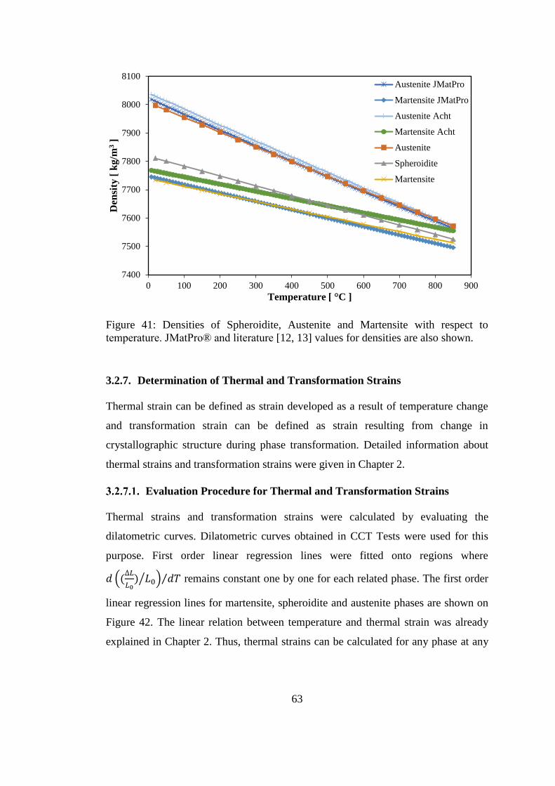
63

Figure 41: Densities of Spheroidite, Austenite and Martensite with respect to

temperature. JMatPro® and literature [12, 13] values for densities are also shown.

3.2.7. Determination of Thermal and Transformation Strains

Thermal strain can be defined as strain developed as a result of temperature change

and transformation strain can be defined as strain resulting from change in

crystallographic structure during phase transformation. Detailed information about

thermal strains and transformation strains were given in Chapter 2.

Evaluation Procedure for Thermal and Transformation Strains

Thermal strains and transformation strains were calculated by evaluating the

dilatometric curves. Dilatometric curves obtained in CCT Tests were used for this

purpose. First order linear regression lines were fitted onto regions where

𝑑 ((∆𝐿

𝐿0) 𝐿0⁄ ) 𝑑𝑇⁄ remains constant one by one for each related phase. The first order

linear regression lines for martensite, spheroidite and austenite phases are shown on

Figure 42. The linear relation between temperature and thermal strain was already

explained in Chapter 2. Thus, thermal strains can be calculated for any phase at any

7400

7500

7600

7700

7800

7900

8000

8100

0 100 200 300 400 500 600 700 800 900

Den

sity

[ k

g/m

3]

Temperature [ °C ]

Austenite JMatPro

Martensite JMatPro

Austenite Acht

Martensite Acht

Austenite

Spheroidite

Martensite

64

given temperature, when both transformation strain and thermal expansion

coefficient values for related phase are known.

Figure 42: Thermal strains of martensite, spheroidite and austenite phases for steel

100Cr6. Transformation strains 𝜀𝐴→𝑀 𝑡𝑟 , 𝜀𝑆→𝐴

𝑡𝑟 and 𝜀𝑆→𝑀𝑡𝑟 also indicated on the figure.

Differences in thermal strains between parent and product phases at room

temperature were also indicated on Figure 42, which give the transformation strain

for related phase transformation. The reference phase was taken as spheroidite

during calculation for transformation strains since all samples were spheroidized and

spheroidite was the initial phase for dilatometric tests.

Transformation strains might also be calculated from density measurements with the

relation (12), when the relative amount of phase constituents are known.

Transformation strain of martensite was calculated in such a way from the density

values using Equation (12).

Results of Calculations for Thermal and Transformation Strains

Thermal strains calculated at temperatures 0°C and 1000 °C were given in Table 12.

Transformation strains calculated at temperatures 20 °C and 850 °C were also given

-1

-0,5

0

0,5

1

1,5

-200 0 200 400 600 800 1000

Rel

. C

ha

ng

e in

Len

gth

[ %

]

Temperature [ °C ]

MartensiteSpheroiditeAustenite

εtr

εtr

S-M

S-A

εtrA-M

65

in Table 13. As it can be seen from the results, experimentally determined

transformation and thermal strain values are similar to values found in the literature

[13].

Table 12: Thermal Strains calculated at 0 °C and 1000 °C.

Temperature: 0 °C 1000 °C

Thermal Strain for Spheroidite [ - ], 𝜀𝑆 𝑡ℎ -3.01*10-4 1.48*10-2

Thermal Strain for Austenite [ - ], 𝜀𝐴 𝑡ℎ -8.28*10-3 1.39*10-2

Thermal Strain for Martensite [ - ], 𝜀𝑀 𝑡ℎ 3.09*10-3 1.48*10-2

Table 13: Transformation Strains calculated at 20 °C and 850 °C.

Temperature: 20 °C 850 °C

Spheroidite to Austenite [%], 𝜀𝑆→𝐴𝑡𝑟 -7.83*10-1 -1.91*10-1

Austenite to Martensite [%], 𝜀𝐴→𝑀 𝑡𝑟 1.12*100 2.44*10-1

Spheroidite to Martensite [%], 𝜀𝑆→𝑀𝑡𝑟 3.32*10-1 5.31*10-2

3.2.8. Determination of Mechanical Properties of Austenite, Martensite and

Bainite Phases

Flow curves for austenite, martensite and bainite phases were determined as a

function of temperature using deformation dilatometry. Ramberg-Osgood Model

(25) has been used in order to introduce stress-strain curves as a function of

temperature into the heat treatment simulation code of SYSWELD®.

𝜎𝑡𝑟𝑢𝑒 = 𝐾𝑅𝑂(𝜀𝑖𝑝𝑙)

𝑛𝑅𝑂 (25)

where, 𝜎𝑡𝑟𝑢𝑒 is the true stress, 𝜀𝑖𝑝𝑙

is the plastic strain, 𝐾𝑅𝑂 and 𝑛𝑅𝑂 values represent

material parameter and strain hardening exponent of Ramberg-Osgood model

respectively.

66

Since the deformation measurement system (LVDT) of the deformation dilatometer

measures total strain one must calculate 𝜀𝑖𝑝𝑙

from total strain and elastic modulus

before fitting the parameters to the model. Assuming an additive decomposition,

total strain can be described as the sum of elastic (𝜀𝑖𝑒𝑙) and plastic (𝜀𝑖

𝑝𝑙) strains as in

Equation (26). Moreover, thermal, transformation and transformation plasticity

strains are not involved in the total strain given in Equation (26) since the

dilatometry tests were conducted isothermally and they were all finished before the

initialization of phase transformation.

𝜀𝑖𝑡𝑜𝑡 = 𝜀𝑖

𝑒𝑙 + 𝜀𝑖𝑝𝑙

(26)

Equation (25) can be rearranged as the following form (27) by using Equation (26):

𝜀𝑖𝑡𝑜𝑡 =

𝜎𝑡𝑟𝑢𝑒

𝐸𝑖+ 𝐾𝑅𝑂 [

𝜎𝑡𝑟𝑢𝑒

𝐸𝑖]

𝑛𝑅𝑂

(27)

where, 𝜀𝑖𝑡𝑜𝑡 represents total strain measured by dilatometer for sample i, 𝜎𝑡𝑟𝑢𝑒 is the

true stress, 𝐸𝑖 is the elastic modulus of sample i, 𝐾𝑅𝑂 and 𝑛𝑅𝑂 values represent

material parameter and strain hardening exponent of Ramberg-Osgood model

respectively.

Evaluation Procedure for Mechanical Tests

True strain-true stress plots were obtained from deformation dilatometry tests and

they were fitted onto Ramberg-Osgood model (25) for each phase at a given

temperature.

At first, true plastic strain component of the dilatometric test was calculated by

Equation (26) since the values for total strain and elastic strain components were

both known. Total strain was obtained from dilatometric tests and elastic strain

component was calculated from dividing total stress to elastic modulus of related

phase at a given temperature. Modulus of elasticity was obtained from JMatPro®

calculations since stiffness of the dilatometer was not adequate for determination of

elastic modulus for steels. After calculating plastic strain component of the

dilatometric test, Ramberg-Osgood model parameters 𝐾𝑅𝑂 and 𝑛𝑅𝑂 were fitted

67

iteratively by reducing total RMS error between plastic strain component of the test

and calculated value from the model. A representative example given in Figure 43

shows a good agreement established between measured data and the fitting.

Figure 43: Ramberg-Osgood Model fitting for mechanical test of austenite at 850°C.

After determining the Ramberg-Osgood parameters for each phase and for each

temperature, the temperature dependency of the parameters 𝐾𝑅𝑂 and 𝑛𝑅𝑂 were

determined by fitting the calculated values onto linear or polynomial regression lines

with a suitable order. This procedure was applied for all phases and results can be

found in following subdivision.

Results of Mechanical Tests

Calculation results and fitted regression lines for material parameter 𝐾𝑅𝑂 were given

in Figure 44, Figure 46 and Figure 48 for austenite, bainite and martensite phases

respectively. Furthermore, temperature dependency of hardening exponent 𝑛𝑅𝑂 and

regression lines fitted were given in Figure 45, Figure 47 and Figure 49 for

austenitic, bainitic and martensitic phases respectively.

0

20

40

60

80

100

120

0 0,002 0,004 0,006 0,008 0,01 0,012 0,014 0,016 0,018

Tru

e S

tres

s σ

[ M

Pa

]

True Plastic Strain ε [ - ]

Ramberg-Osgood Fitting

Experiment

68

In mechanical test of meta-stable austenite, flow-curves were obtained for a

temperature range between 300°C to 850°C since martensite start temperature was

calculated as 212±1 °C and below 300°C, austenite might be transformed into

martensite. In order to describe mechanical properties of austenite below 300°C,

fittings of calculated 𝐾𝑅𝑂 and 𝑛𝑅𝑂 values for a temperature range 300°C-850°C were

extrapolated to room temperature.

In mechanical tests of martensitic and bainitic phases it was aimed to reach at least

%1 strain at elevated temperatures, however dilatometer was not able to reach

required stress level for %1 strain for both martensitic and bainitic phases even at the

elevated temperatures. Furthermore, martensitic and bainitic phases could not have

plastically deformed below 300 °C since the force needed for plastic deformation of

martensitic and bainitic phases is much higher than the force that is able to be

applied by dilatometer. Therefore, experiments conducted below 300 °C temperature

was not taken into consideration for determination of mechanical properties of

martensitic and bainitic phases.

In consequence, fittings of calculated 𝐾𝑅𝑂 and 𝑛𝑅𝑂 values for a temperature range

above 300°C were extrapolated to room temperature in order to investigate

mechanical properties of martensitic and bainitic phases. It must be noted that the

results given in this section only applicable up to %1 strain for martensitic and

bainitic phases.

Dashed lines shown on the figures are referred as the extrapolated regions due to

above mentioned problems in order to describe and investigate the tendency of 𝐾𝑅𝑂

and 𝑛𝑅𝑂.

As it can be seen from the Figure 44, Figure 46 and Figure 48, calculated values for

material parameter 𝐾𝑅𝑂 show a linear relationship with temperature. On the other

hand, hardening exponent 𝑛𝑅𝑂 values do not have clear relationship with temperature

as it can be seen in Figure 45, Figure 47 and Figure 49.

69

Figure 44: Results of calculations for

mechanical tests of austenite and

regression line fitted for material

parameter 𝐾𝑅𝑂 w.r.t. temperature.

Figure 45: Temperature dependency of

hardening exponent 𝑛𝑅𝑂 and regression

line fitted onto calculated values of

mechanical tests of austenite.


mechanical tests of bainite and regression

line fitted for material parameter 𝐾𝑅𝑂

w.r.t. temperature.




mechanical tests of bainite.


mechanical tests of martensite and

regression line fitted for material

parameter 𝐾𝑅𝑂 w.r.t. temperature.




mechanical tests of martensite.

0

200

400

600

800

1000

1200

0 100 200 300 400 500 600 700 800 900

K [

MP

a ]

Temperature [ °C ]

0

0,05

0,1

0,15

0,2

0 100 200 300 400 500 600 700 800 900

n [

-]

Temperature [ °C ]

0

2000

4000

6000

8000

0 100 200 300 400 500 600 700

K [

MP

a ]

Temperature [ °C ]

0

0,05

0,1

0,15

0,2

0,25

0 100 200 300 400 500 600 700

n [

-]

Temperature [ °C ]

0

1000

2000

3000

4000

5000

0 100 200 300 400 500

K [

MP

a ]

Temperature [ °C ]

0

0,05

0,1

0,15

0,2

0 100 200 300 400 500

n [

-]

Temperature [ °C ]

70

Flow curves calculated from Ramberg-Osgood model with 𝐾𝑅𝑂 and 𝑛𝑅𝑂 fittings for

austenitic, bainitic and martensitic phases were given as a function of temperature in

Figure 50, Figure 51 and Figure 52 respectively. Flow curves found in the literature

[12] are also indicated on the same figures in order to make a comparison between

them.

Calculated flow curves for meta-stable austenite are in good agreement with flow

curves available in the literature [12] as it can be seen in Figure 50. Calculated flow

curve for martensite also compared in Figure 52 with flow curve found in the same

literature. Flow curves for martensite are converging quite well at elevated

temperatures, while they are diverging with decreasing temperature.

Figure 50: True stress vs. true plastic strain plots for meta-stable austenite for a

temperature range 300°C-850°C. Flow curves from the literature [12] are also

indicated.

0

50

100

150

200

250

300

350

400

450

500

0 0,005 0,01 0,015 0,02

Tru

e S

tres

s σ

[ M

Pa ]


300 - Literature

400 - Literature

500 - Literature

600 - Literature

700 - Literature

850 - Literature

300 - Experiments

400 - Experiments

500 - Experiments

600 - Experiments

700 - Experiments

850 - Experiments

71

Figure 51: True stress vs. true plastic strain plots for bainitic phase for a temperature

range 100°C-600°C.

Figure 52: True stress vs. true plastic strain plots for martensitic phase for a

temperature range 100°C-450°C. Flow curves found in literature [12] are also

indicated.

0

500

1000

1500

2000

2500

3000

3500

0 0,005 0,01 0,015 0,02

Tru

e S

tres

s σ

[ M

Pa

]


100 - Experiments

200 - Experiments

300 - Experiments

400 - Experiments

500 - Experiments

600 - Experiments

0

500

1000

1500

2000

2500

3000

3500

0 0,005 0,01 0,015 0,02

Tru

e S

tres

s σ

[ M

Pa ]


100 - Literature200 - Literature300 - Literature400 - Literature450 - Literature100 - Experiments200 - Experiments300 - Experiments400 - Experiments450 - Experiments

72

Yield strengths, 𝜎𝑦, of austenitic, bainitic and martensitic phases were calculated in

accordance with Ramberg-Osgood equation (25) at 0.005% proof stress (28):

𝜎𝑦 = 𝐾𝑅𝑂(0.00005)𝑛𝑅𝑂 (28)

Results were given in Figure 53, Figure 54 and Figure 55. Yield strengths found in

the literature and values computed via JMatPro® are also indicated on the same

figures. Furthermore, both linear and second order polynomial fittings were tested

and they are indicated on the figures. However, linear fittings were taken into

consideration since they have reasonable values when compared with second order

polynomial fittings in terms of their extrapolated values at room temperature.

As it can be seen from the figures, experimentally determined yield strengths for

meta-stable austenite and martensite are in good agreement with the literature. On

the other side, computed yield strengths via JMatPro® are showing different

tendency from both experimental and literature values since it does not include

fracture mechanisms in computations.

Figure 53: Yield strengths of meta-stable austenite as a function of temperature.

Yield strengths found in literature and computed via JMatPro® are also indicated.

0

50

100

150

200

250

300

350

400

450

0 100 200 300 400 500 600 700 800 900

Yie

ld S

tres

s [

Mp

a ]

Temperature [ °C ]

Data Points

Acht

JMatPro

Extrapolation of Polynomial Fitting

2nd Order Polynomial Fitting

Extrapolation of Linear Fitting

Linear Fitting

73

Figure 54: Yield strength of bainitic

phase with respect to temperature.

Figure 55: Yield strength of martensitic

phase as a function of temperature.

3.2.9. Determination of the Effect of Stress on Phase Transformations

In this part of the study, the effect of uniaxial compressive stresses on bainitic and

martensitic phase transformations was aimed to be investigated with stressed

dilatometry. As it can be seen from Equation (4), transformation plasticity is

characterized with transformation plasticity parameter (𝐾𝑡𝑝) which was calculated

with an evaluation procedure given in following section.

Evaluation Procedure for TRIP Tests

Difference between longitudinal strains of stress-free sample and stressed one for the

related transformation gives the transformation plasticity. The relationship was

defined in Equation (29) for a given temperature:

𝜀𝑡𝑝(𝑃) = 𝜀(𝜎, 𝑃) − 𝜀(𝜎 = 0, 𝑃) (29)

where, P is the fraction of phase and transformation of related phase is finished when

P = 1, which means the transformation plasticity has its maximum value and often

called as extent of transformation plasticity.

In order to investigate the effect of stress on bainitic phase transformation, applied

stress and temperature were held constant during the test until phase transformation

was completed. Therefore, extent of transformation was taken into account in

calculations since the phase transformation was completed. Difference between

longitudinal strains of stress-free sample and stressed ones for the bainitic

transformation can be seen in Figure 56. Relative change in length versus time

0

500

1000

1500

0 100 200 300 400 500 600 700

Yie

ld S

tres

s [

MP

a ]

Temperature [ °C ]

JMatProData PointsExtrapolationLinear Fit

0

500

1000

1500

2000

2500

3000

0 100 200 300 400 500

Yie

ld S

tres

s [

MP

a ]

Temperature [ °C ]

Data PointsLiteratureJMatProPolynomial fitLinear fit

74

curves were obtained from stressed dilatometry tests. The raw data obtained from the

tests fitted onto JMA equation as described in TTT tests for theoretical calculation of

end points of bainitic phase transformations at different stress levels.

Figure 56: The effect of stress on bainitic phase transformation.

In order to investigate the effect of stress on martensitic phase transformation,

various uniaxial stresses were applied to the specimens at 350°C and held constant

during cooling to the room temperature with 10°C/s cooling rate. It is expected that

martensitic phase transformation could not be completed at room temperature since

Mf calculated as -94±1 °C. Progress of transformation plasticity function f(z) must be

introduced for calculation of transformation strain as in the Equation (4) when phase

transformation is not completed. However, progress of transformation plasticity

function would be subtracted from the equation if strain at the end of phase

transformation is known. Therefore, modified Koistinen-Marburger equation (22)

was fitted onto dilatometric curves then the curves were extrapolated according to

their modified Koistinen-Marburger fittings until completion of their transformations

(99.9%). Longitudinal strains at the extrapolated end for each stress levels were

-0,05

0,05

0,15

0,25

0,35

0,45

10 40 70 100 130 160 190 220 250 280 310 340 370 400 430 460

Rel

ati

ve

Ch

an

ge

in L

eng

th [

% ]

Time [ s ]

0 MPa5 MPa20 MPa40 MPa50 MPa

75

obtained from these fittings. In order to fit the modified equation phase fractions

must be obtained by applying lever rule to the dilatometric curve as discussed before.

Thus, thermal strains for austenitic and martensitic phases were calculated for each

test in order to apply the lever rule. Thermal strain of austenite was calculated from

the test. However, thermal strain for martensitic phase was not known since

martensitic transformation was not completed. In order to determine thermal strain of

martensite for each test, retained austenite values of specimens measured and

iteratively matched for giving same results with lever rule. The amount of retained

austenite present in the specimens was measured via XRD. In consequence,

dilatometric curves obtained from the TRIP tests and extrapolated curves (dashed

lines) can be seen in Figure 57.

Figure 57: Modified Koistinen-Marburger fitted dilatometric curves of TRIP tests of

martensitic transformation. Extrapolated regions are indicated as dashed lines.

Results of TRIP Tests

Transformation plasticity strain versus applied stresses for both bainitic and

martensitic phase transformations are given in Figure 58 and Figure 59 respectively.

-0,3

-0,2

-0,1

0

0,1

0,2

0,3

-150 -100 -50 0 50 100 150 200 250 300

Rel

ati

ve

Ch

an

ge

in L

ength

[

% ]

Temperature [ °C ]

0 MPa - Experiment

5 MPa - Experiment

50 MPa - Experiment

100 MPa - Experiment

76

It must be noted that, TRIP tests were performed at temperature of 350 °C under

various uniaxial compression stresses as explained before. Therefore, results are only

applicable for 350 °C and uniaxial compression stresses within a range 0 MPa to 100

MPa.

As it can be seen from Figure 58 and Figure 59 , transformation plasticity strains

(𝜀𝑡𝑝) have linear relationship with the applied stresses for both bainitic and

martensitic phase transformations. The slope of the straight lines indicated on the

figures can be commented as transformation plasticity parameter (𝐾𝑡𝑝) as stated in

Equation (4). The transformation plasticity parameter was calculated as 1.06*10-5

MPa-1 and 6.82*10-5 MPa-1 for martensitic and bainitic phase transformations

respectively.

Figure 58: Transformation plasticity

strain vs. applied load plot for bainitic

phase transformation.

Figure 59: Transformation plasticity

strain vs. applied load plot for martensitic


In addition to experimental determination of 𝐾𝑡𝑝, there are models available for the

calculation of 𝐾𝑡𝑝 in the literature [29, 55, 57, 58]. Greenwood and Johnson were

published their model (30) in 1965. After the work published by Greenwood and

Johnson, Abrassart (31), Leblond (32) and Dalgic (33) were developed models for

the calculation of 𝐾𝑡𝑝 which are mainly based on the former model of Greenwood

and Johnson. The models are given as follows:

𝐾𝑡𝑝 =5

6∙

1

𝜎𝑦𝑎 ∙

∆𝑉

𝑉 (30)

-0,004

-0,003

-0,002

-0,001

0

-60 -40 -20 0

εtp

σapp [ MPa ]

0

0,0002

0,0004

0,0006

0,0008

0,001

0,0012

-150 -100 -50 0

εtp

σapp [ MPa ]

77

𝐾𝑡𝑝 =1

4∙

1

𝜎𝑦𝑎 ∙

∆𝑉

𝑉 (31)

𝐾𝑡𝑝 =2

3∙

1

𝜎𝑦𝑎 ∙

∆𝑉

𝑉 (32)

𝐾𝑡𝑝 = 𝑐 ∙1

𝜎𝑦𝑎 ∙

∆𝑉

𝑉 (33)

where, 𝜎𝑦𝑎 is the yield strength of austenite at a given temperature,

∆𝑉

𝑉 is the volume

change during phase transformation and c is temperature dependent factor for the

model developed by Dalgic and it may take a value between 0.25 and 0.83. As it can

be seen from the equations, the models mainly related with yield strength of

austenite and change in volume due to phase transformation.

Models were tested and the results for martensitic phase transformation are given in

Figure 60. In order to calculate 𝐾𝑡𝑝 with these models, volume change and yield

strength of austenite must be known as a function of temperature. The change in

volume was obtained from the dilatometric tests performed for TRIP tests of

martensitic phase. Change in volume could not be measured by the dilatometer since

dilatometer has only one extensometer which is used for measuring longitudinal

strains of the specimen. Therefore, change in volume was calculated by longitudinal

strains obtained from the dilatometric tests with following relation (34):

∆𝑉

𝑉= 3

∆𝑙

𝑙 (34)

Yield strength of austenite had been already determined as a function of temperature

in mechanical tests of meta-stable austenite. After calculation of 𝐾𝑡𝑝 as a function of

temperature with the theoretical models, integral sum of the curves given in Figure

60 were taken and calculated values determined as 𝐾𝑡𝑝 value for a temperature range

between 0°C to 210°C. However, the integral sum, which was calculated from the

model developed by Leblond, was determined as 𝐾𝑡𝑝 value for martensitic

transformation since SYSWELD® is using Leblond model for calculation of

transformation plasticity constant.

78

Figure 60: Theoretically calculated transformation plasticity parameter vs.

temperature plot for martensitic phase transformation.

Experimentally determined and theoretically calculated values of transformation

plasticity constants for both bainitic and martensitic phases are given in Table 14.

Values found in the literature [58] for 𝐾𝑡𝑝 are also given in the same table. As it can

be seen from the Table 14, results for bainitic transformation are good agreement

while results for martensitic transformation are not. The difference observed in the

results for martensitic transformation could be due to difference in calculation

procedures or in experimental conditions.

Table 14: Results for calculations of transformation plasticity constants of bainitic

and martensitic phases at 350 °C.

Phase Experimental Theoretical Literature

Bainite [10-5 MPa-1] 6.82 5.08 7,24

Martensite [10-5 MPa-1] 1.06 1.32 5,42

Experimentally and theoretically determined 𝐾𝑡𝑝 values were tested in a through-

hardening simulation of a conical ring and results are given in Chapter 5.

0

1

2

3

4

5

6

0 50 100 150 200 250

Tra

nsf

orm

ati

on

Pla

stic

ity

Pa

ra

met

er

Ktp

[ 1

0-5

Mp

a ]

Temperature [ °C ]

Greenwood 5/6 K [ MPa ] Dalgic 0.25 K [ MPa ]

Abrassart 1/4 K [ MPa ] Dalgic 0.83 K [ MPa ]

Leblond 2/3 K [ MPa ] Literature

Experimental

79

CHAPTER 4

COMPUTATIONAL DETERMINATION OF MATERIAL PROPERTIES

4. COMPUTATIONAL DETERMINATION OF MATERIAL PROPERTIES

4.1. General

Determination of material properties in order to use in through-hardening

simulations was aimed in this study. In addition to experimentally determined

material properties in the previous chapter, several properties are also needed for

through-hardening simulations such as specific heat, thermal conductivity, enthalpy,

Young’s modulus and Poisson’s ratio. The effect of these properties on through-

hardening simulations is negligible as experienced in preliminary study. However,

simulations cannot be initialized without these material properties. Therefore,

density, specific heat, thermal conductivity, enthalpy, Young’s modulus and

Poisson’s ratio values for steel 100Cr6 were intended to be calculated with

computational methods.

4.2. Theory

Computational techniques for material property determination is undergoing a rapid

development. Phase constitution as a function of temperature and chemical

composition might be calculated with traditional thermodynamics. However, there

exist a separation of material properties and the thermodynamic properties. There is

currently available software namely, JMatPro®, which enhances the thermodynamic

calculations to make quantitative calculations possible with physical and

microstructural parameters and the material properties [15]. The quantitative

calculation for the requested material property is obtained via thermodynamic

calculations by taking into account of theoretical material models and property

databases. In multicomponent systems, material properties needed such as Young’s

80

modulus, Poisson’s ratio and densities are calculated by pair wise mixture models for

each phase.

Material properties are well calculated with using computational techniques, there

are a lot of work published that JMatPro® had been used for calculation of material

properties and works also consist of verification of computational results with

corresponding experiments [15-20, 66-68]. Calculation procedure for material

properties of any steel can be summarized in four steps (Figure 61).

Figure 61: Calculation procedure for material property and methods used for each

calculation step.

At first, chemical composition of the steel is used as an input data for the software.

Then, CALPHAD method is used in order to determine fractions of phases. Basic

Calculate Constituents of

Microstructure

Calculate Physical Properties

of each Constituent

Calculate Final Properties

via Physical Models

METHODS Thermodynamic Theories

(CALPHAD) Kinetic Theory

Diffusion Theory

METHODS Dislocation Mechanics

Micro-Mechanics

Continuum Mechanics

Internal State Variable

Models

Representative Volume

Element Methods

METHODS Thermodynamics based physical

properties calculations Quantum Mechanics

Atomistic Simulations

MD

DFT

Calculate Composition of

Constituents

81

principle of CALPHAD method is the minimization of excess free energy which can

be expressed as follows (35):

𝐺 = ∑ 𝑋𝑖𝐺𝑖0 +

𝑖

𝑅𝑇 ∑ 𝑋𝑖 ln 𝑋𝑖

𝑖

+ ∑ ∑ 𝑋𝑖𝑋𝑗

𝑗>𝑖𝑖

∑ 𝜑𝑣(𝑋𝑖 − 𝑋𝑗)𝑣

𝑣

(35)

where, i and j are element indexes in a phase, G0 is the Gibbs free energy of pure

components, 𝜑𝑣 is interaction terms (based on pairwise interactions), Xi and Xj are

the mole fractions of elements i and j.

In the third step, determination of properties of each phase is done with

thermodynamic based material property calculation. JMatPro® uses basic equation

for the Gibbs free energy of a multi-component solution phase, which includes Gibbs

free energy of pure components, ideal entropy and interaction terms as expressed in

Equation (35). Model that is used in JMatPro® is analogue and based on the Gibbs

free energy equation. Interaction parameter is same but not identical with the

analogue one as given in Equation (36):

𝑃 = ∑ 𝑋𝑖𝑃𝑖0 +

𝑖

∑ ∑ 𝑋𝑖𝑋𝑗

𝑗>𝑖𝑖

∑ 𝜔𝑖𝑗𝑣 (𝑋𝑖 − 𝑋𝑗)𝑣

𝑣

(36)

where, P is the material property, i and j are element indexes in a phase, P0 is the

property of the phase in the pure element, 𝜔𝑖𝑗𝑣 is a binary interaction parameter, Xi

and Xj are the mole fractions of elements i and j.

At the last step of calculation, property of phase mixture is determined by composite

theory. Calculation starts for each individual phase then final mixture of phases can

be determined by mixture models given in Equations (37) and (38) which is taking

into account of the effect of microstructure on final material property. For upper

bound of mixture model, following Equation (37) is used;

𝑃𝑚𝑖𝑥 = ∑ 𝑋𝑖𝑃𝑖

𝑖=𝑗

𝑖=1

(37)

and for lower bound Equation (38) is used;

82

1

𝑃𝑚𝑖𝑥= ∑

𝑋𝑖

𝑃𝑖

𝑖=𝑗

𝑖=1

(38)

where, 𝑃𝑚𝑖𝑥 is the property of mixture, i and j are element indexes in a phase and Xi

is the mole fraction of elements i.

4.2.1. Calculation of TTT and CCT diagrams

Furthermore, the code is able to calculate TTT and CCT diagrams almost accurate

for general steels, including medium to high alloy steels, tool steels and 13%Cr

steels [19, 68]. Thermodynamic models together with kinetic phase transformation

models is used for in case of calculating TTT and CCT diagrams. The model used

for transformation mainly based on the model developed by Kirkaldy [69] and co-

workers. The modified model of Kirkaldy is given in Equation (39):

𝑡(𝑃, 𝑇) =1

𝛼(𝑁)∆𝑇𝑞𝐷∫

𝑑𝑃

𝑃2(1−𝑃) 3⁄ (1 − 𝑃)2𝑃 3⁄

𝑃

0

(39)

where, 𝛼(𝑁) = 𝛽(𝑁−1) 2⁄ and β is an empirical coefficient, N is the ASTM grain size

D is an effective diffusion coefficient ΔT is the undercooling below the temperature

where austenite is unstable with respect to ferrite, q is an exponent dependent on the

effective diffusion mechanism, and P is the fraction transformed.

Once the TTT diagram is calculated it can be transformed into a CCT diagram by the

rule of additivity as mentioned in Chapter 2 [68-71]. There are several works

published about determination of TTT and CCT diagrams by JMatPro® and their

comparison with corresponding experimental results and the literature [19, 68, 72].

4.3. Calculation and Evaluation Procedure

Chemical composition of the material required in order to calculate material

properties with calculation procedure mentioned in previous sub-division. Therefore,

calculations were based on chemical composition of 100Cr6 as given in Table 2.

Grain size was taken as 7.4 ASTM and austenitization temperature was taken as 850

°C at first. The composition of the austenite present at this temperature is calculated

83

directly by taking into account of carbide and other second phases present at this

quenching temperature. Thus, the code fails in a partial austenitization case. It

assumes the case is in the cementite transition temperature so that it calculates 1.81

Wt.% cementite and 98.17 Wt.% austenite present in the microstructure. After then,

the code calculates transformation for austenite was taken place in equilibrium at 850

°C for 98.17Wt% austenitic microstructure. Furthermore, it neglects the dissolution

of carbide particles during the austenitization which can affect and change the

martensite start temperature. As a solution, a trick was suggested by developers of

the code in order to achieve similar austenitization condition as in dilatometric tests.

The trick is related with martensite start temperature which was determined

experimentally and supposed to be calculated also by the code as 212±1 °C. If the

martensite start temperature will able to be obtained at the end of calculation, it can

be commented as the amount of austenite decomposed is same with the

corresponding dilatometric tests. That’s why, martensite start temperature obtained

in calculations must be same the temperature obtained from the dilatometric tests. It

can be done by changing quenching temperature. Therefore, austenitization

temperature was chosen as 812 °C in order to obtain same martensite start

temperature with dilatometric tests.

The code computed weight fractions of phases 3.46 Wt.% and 96.52 Wt.% in the

microstructure at 812 °C for the cementite and austenite phases respectively.

Uniform cooling with a 10 °C/s cooling rate was chosen for quenching properties.

4.4. Results

The effect of diminutive differences in chemical composition on thermo-physical

properties were also investigated. Consequently, it was observed that the effect is not

significant as it can be seen from the results given in Figure 62.

The difference in compositions can be seen in Table 15. “Composition 1” is the

composition used in this study and “Composition 2” is the standard composition for

100Cr6.

84

Table 15: Compositions used for computational part of the study.

C Cr Si Mn Al Cu Mo Ni O P

Composition 1 0.99 1.43 0.24 0.36 0.017 0.1 0.02 0.06 5e-5 0.016

Composition 2 0.99 1.47 0.25 0.35 0.050 0.3 0.1 0.1 15e-4 0.025

Figure 62: Comparison of phase amounts between diminutive differences in

chemical composition of steel 100Cr6. “Composition 1” is the composition used in

this study and “Composition 2” is standard composition for 100Cr6.

Thermo-physical properties, density, specific heat, thermal conductivity, enthalpy,

Young’s modulus and Poisson’s ratio, were computed for each phase and results

were given in Figure 63, Figure 64, Figure 65, Figure 66, Figure 67 and Figure 68

respectively as graphical representations. Data available in the literature [12, 13]

were also indicated on the figures in order to make a comparison with computed

results. From these figures, it can be commented that good agreements for the

properties, density, specific heat, thermal conductivity and enthalpy, have been

established between the computed results and the literature.

0

10

20

30

40

50

60

70

80

90

100

0 100 200 300 400 500 600 700

Ph

ase

s V

olu

me

[ %

]

Temperature [ °C ]

Composition 1 - Martensite

Composition 1 - Austenite

Composition 2 - Martensite

Composition 2 - Austenite

85

On the other side, Young’s modulus and Poisson’s ratio for the austenitic phase

different from the literature as in Figure 67 and Figure 68. This is due to instrument

used for measuring the dilation during mechanical tests in the experimental work of

Acht et. al. [12]. Stiffness of the instrument and the method for measuring the

dilation of the specimen may affect the flow curve measured. It is highly doubted

that the measured data in the experiments they performed consists of the dilation of

the punches and other components of the instrument itself as in experiments

performed in this study.

TTT and CCT diagrams computed according to ASTM grain size 7.4 and

austenitization temperature was taken as 812 °C due to problems mentioned above.

Results were given in Chapter 3 together with experimentally determined diagrams

and diagrams found in the literature.

Figure 63: Comparison of density values computed (solid) and found in the literature

(dashed) for martensitic and austenitic phases as a function of temperature.

7400

7500

7600

7700

7800

7900

8000

8100

0 100 200 300 400 500 600 700 800 900

Den

sity

[ k

g/m

3 ]

Temperature [ °C ]

JMatPro - Martensite

JMatPro - Austenite

Literature - Martensite

Literature - Austenite

86

Figure 64: Specific heat for each phase of 100Cr6 with respect to temperature.

Figure 65: Thermal conductivity for each phase of 100Cr6 with respect to

temperature.

0

200

400

600

800

1000

1200

1400

1600

0 100 200 300 400 500 600 700 800 900

Sp

ecif

ic H

eat

Ca

pa

city

[ J

/kg

·°C

]

Temperature [ °C ]


JMatPro - Austenite



0

0,005

0,01

0,015

0,02

0,025

0,03

0,035

0,04

0,045

0,05

0 100 200 300 400 500 600 700 800 900

Th

erm

al

Con

du

ctiv

ity [

W /

mm

·°C

]

Temperature [ °C ]


JMatPro - Austenite



87

Figure 66: Enthalpy for each phase of 100Cr6 with respect to temperature.

Figure 67: Young's modulus for each phase of 100Cr6 with respect to temperature.

0

100000

200000

300000

400000

500000

600000

700000

0 100 200 300 400 500 600 700 800 900

En

tha

lpy

[ J

/kg

]

Temperature [ °C ]




JMatPro - Austenite

0

50000

100000

150000

200000

250000

300000

0 100 200 300 400 500 600 700 800 900

You

ng's

Mod

ulu

s [

Mp

a ]

Temperature [ °C ]


JMatPro - Austenite



88

Figure 68: Poisson’s ratio for each phase of 100Cr6 with respect to temperature.

Additionally, thermo-physical properties for the soft phase were also computed with

JMatPro®. However, their results were not given in these graphical representations

since they were summarized in Table 16, Table 17 and Table 18 as polynomials with

respect to temperature. The values given in Table 16, Table 17 and Table 18 for

related material properties must be used with following relation (40):

𝑃(𝑇) = 𝐴𝑜 + 𝐴1𝑇1 + 𝐴2𝑇2 + 𝐴3𝑇3 + 𝐴4𝑇4 (40)

where, P(T) is the material property at a given temperature, T is temperature and An

is the constant for related material property which is given in Table 16, Table 17 and

Table 18.

0

0,05

0,1

0,15

0,2

0,25

0,3

0,35

0,4

0,45

0,5

0 100 200 300 400 500 600 700 800 900

Pois

son

's R

ati

o [

-]

Temperature [ °C ]


JMatPro - Austenite



89

Table 16: Summary for calculated and determined Thermo-Physical Properties.

Property Phase A0 A1 A2 A3 A4

Specific Heat

Capacity

[ J/kg·°C ]

Martensite 436.51 0.4875 -6.16*10-04 1.62*10-06

Austenite 448.67 0.3007 -2.49*10-04 1.42*10-07

Enthalpy

[ J/kg ]

Martensite 55776.99 436.65 2.42*10-01 -1.99*10-04 3.99*10-07

Austenite 147540.57 450.35 1.45*10-01 -7.68*10-05 3.37*10-08

Spheroidite -17.59 0.4354 2.20*10-04 -1.21*10-07 2.43*10-10

Thermal

Conductivity

[ W / mm·°C ]

Martensite 0.0393 2.40*10-05 -6.43*10-08

Austenite 0.0168 1.19*10-05

Density

[ kg/m3 ]

Martensite 7738.13 -0.2661

Austenite 8005.31 -0.5136

Spheroidite 7816.67 -0.3443

Thermal Strain with

Transformation

Strain, Tref 20°C [ - ]

GKZ to M -8.28*10-03 2.22*10-05

GKZ to A 3.09*10-03 1.17*10-05

Transformation

Strain, Tref 20°C [%]

GKZ to M* 0.3325

GKZ to A** -0.7835

A to M*** 1.1160

M: Martensite, A: Austenite, GKZ: Spheroidite, (*) GKZ to M: Spheroidite to

Martensite Transformation, (**) GKZ to A: Spheroidite to Austenite

Transformation, (***) A to M: Austenite to Martensite Transformation.

Table 17: Summary for calculated and determined Thermo-Mechanical Properties.

Property Phase A0 A1

Ramberg-Osgood Parameter nRO [ - ]

Martensite 7.97*10-02 1.27*10-04

Austenite 1.22*10-01 3.88*10-05

Bainite 1.58*10-01 4.44*10-05

Ramberg-Osgood Parameter KRO [ MPa ]

Martensite 4.35*10+03 -4.11

Austenite 1.06*10+03 -1.09

Bainite 6.73*10+03 -8.74

Coefficient of Thermal Expansion α [ 10-6 °C-1 ]

Martensite 11.69

Austenite 22.19

Spheroidite 15.06

Young's Modulus E [ MPa ] Martensite 2.12*10+05 -5.27*10+01

Austenite 2.04*10+05 -9.10*10+01

Poisson’s Ratio [ - ] Martensite 0.344 0.0001

Austenite 0.223 0.00025

90

Table 18: Summary for calculated and determined Thermo-Metallurgical Properties.

Property Phase A0

Critical Temperatures for GKZ to A Transformation [ °C ]

Ac1 773.4

Ac3 817.3

Ms Temperature (Ref. transformation at %0.7) [ °C ] A to M*** 212 ± 1

Mf Temperature (Ref. transformation at %99.9) [ °C ] A to M -94 ± 1

Koistinen-Marburger Constant Ω [ - ] A to M 102.001

Koistinen-Marburger Exponent n [ - ] A to M 1.455

Transformation Plasticity Constant Ktp [ 1/MPa ]

A to M 1.06*10-05

A to M (Theoretical) 1.32*10-05

A to B**** 6.82*10-05

M: Martensite, A: Austenite, B: Bainite, (***) A to M: Austenite to Martensite

Transformation, (****) A to B: Austenite to Bainite Transformation.

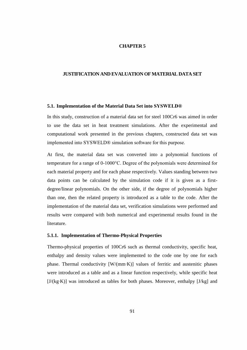
91

CHAPTER 5

JUSTIFICATION AND EVALUATION OF MATERIAL DATA SET

5. JUSTIFICATION AND EVALUATION OF MATERIAL DATA SET

5.1. Implementation of the Material Data Set into SYSWELD®

In this study, construction of a material data set for steel 100Cr6 was aimed in order

to use the data set in heat treatment simulations. After the experimental and

computational work presented in the previous chapters, constructed data set was

implemented into SYSWELD® simulation software for this purpose.

At first, the material data set was converted into a polynomial functions of

temperature for a range of 0-1000°C. Degree of the polynomials were determined for

each material property and for each phase respectively. Values standing between two

data points can be calculated by the simulation code if it is given as a first-

degree/linear polynomials. On the other side, if the degree of polynomials higher

than one, then the related property is introduced as a table to the code. After the

implementation of the material data set, verification simulations were performed and

results were compared with both numerical and experimental results found in the

literature.

5.1.1. Implementation of Thermo-Physical Properties

Thermo-physical properties of 100Cr6 such as thermal conductivity, specific heat,

enthalpy and density values were implemented to the code one by one for each

phase. Thermal conductivity [W/(mm∙K)] values of ferritic and austenitic phases

were introduced as a table and as a linear function respectively, while specific heat

[J/(kg∙K)] was introduced as tables for both phases. Moreover, enthalpy [J/kg] and

92

density [kg/mm3] values of ferritic, martensitic and austenitic phases were defined to

the code as tables.

5.1.2. Implementation of Thermo-Metallurgical Properties

Thermo-metallurgical properties of 100Cr6 were implemented as phase

transformation data for each phase in accordance with metallurgical models defined

in the code. The code includes JMA and Leblond metallurgical models and these

models might be used for diffusional phase transformations. Furthermore, for

displacive phase transformations, Koistinen-Marburger model had been implemented

to the code and it can be used with diffusional models simultaneously. However, as

mentioned in Chapter 3, Koistinen-Marburger model was not giving good results at

the room temperature when compared with the experimental results. That’s why,

Koistinen-Marburger model was modified in order to give better results as discussed

in Chapter 3. SYSWELD® is giving an opportunity to users that transformation

kinetics can be defined with Simplified Fortran codes by user. However, the user-

programmed transformation kinetics cannot be used together with metallurgical

transformation models included in the code. The code also has a shared library

USMETA routine which includes metallurgical transformation model of JMA.

Modified Koistinen-Marburger model was added onto USMETA routine in order to

solve this problem. However, there is no need to use diffusional phase

transformation models for the case given in following sub-division since only

martensitic phase transformation is expected to be occurred due to given quenching

conditions. Therefore, only modified Koistinen-Marburger model was defined to the

code as a transformation model by Simplified Fortran program.

5.1.3. Implementation of Thermo-Mechanical Properties

Thermo-mechanical properties of 100Cr6 such as elastic modulus, Poisson’s ratio,

thermal strain, yield strength and hardening behavior of the steel were defined to the

code separately for each related phase. Elastic modulus [MPa], Poisson’s ratio [-]

and thermal strains [1/°C] for austenitic and martensitic phases were defined as

linear polynomials while yield strength [MPa] for each phase introduced as tables.

Furthermore, hardening behavior of austenitic and martensitic phases were

93

implemented to code as tables at a given temperatures by extracting the yield

strength value from nominal stress values of related phase. Transformation plasticity

constant, 𝐾𝑡𝑝, was defined as constant value for all phases since the code assumes

transformation plasticity is equal for all phases.

5.2. Through-Hardening Simulation for Conical Bearing Ring

In this part, through-hardening process for outer ring of conical bearing was studied.

Verification of the data set performed for the through-hardening simulation of the

conical bearing ring and results were compared with numerical results obtained by

Acht [13].

Acht et al. [13] had been studied through-hardening process of conical bearing ring

which was made from 100Cr6 and dimensions of the outer ring were given in Figure

69. Furthermore, they have supported their numerical results with experimental

results. In performed simulations, same process parameters and conditions were used

as in the work of Acht et al. in order to make a meaningful comparison.

Figure 69: Conical bearing ring used in through-hardening simulation.

94

5.2.1. Details of Simulation

For verification of the data set, simulations were performed with finite element

software code, SYSWELD®, using 2-D axi-symmetrical option with isotropic strain

hardening model.

First step for the simulation is meshing of the geometry. Half of the ring is modelled

in 2-D since axi-symmetrical option is used. The mesh given in Figure 70 has been

generated manually, then it was subdivided via automatic mesher. Important nodes,

which are used as data points for comparison of the simulation results, are also

indicated on the same figure with boundary conditions.

Element type was selected as 8-noded quadrilateral elements with reduced

integration since it is known that quadrilateral type of elements are giving good

results when compared with 4-noded elements in the case of bending load by

avoiding shear locking. Moreover, in order to reduce computation time and

efficiency, reduced integration is used with quadrilateral elements. There are 1300

quadrilateral elements with 4071 nodes used in the simulations.

As an initial condition, it is also assumed that component has a homogenous

temperature distribution through-out its cross-section with austenitic microstructure.

Therefore, %100 austenitic phase was defined as an initial phase for all of the

elements and all of the nodes.

The conical bearing ring was quenched to the room temperature from a temperature

of 850 °C inside a gas nozzle field. Heat transfer coefficients for the gas flow over

the component were taken as 444 W/(m2K) for sides, 205 W/(m2K) for bottom face,

and 317 W/(m2K) for the top face of the conical ring.

Boundary conditions for heat transfer coefficients are shown in Figure 70 as blue

arrows. Clamping applied on the ring in y-direction, Uy=0, is also shown in the same

figure as a red arrow.

95

Figure 70: The mesh used in simulations. Boundary conditions (arrows) and

important nodes (+) are also indicated. #1 bottom side, #2 core, #3 inner side, #4

outer side, #5 group of nodes represented as line and #6 top side.

5.2.2. Results

Cooling Curves

A comparison of cooling curves with the literature is given in Figure 71. Detailed

view of the same figure is given in Figure 72. As it can be seen from the Figure 71,

cooling curves obtained from simulation and cooling curves given in the literature

are in good agreement regardless of the position of nodes.

96

Figure 71: Comparison of cooling curves obtained from simulations with literature.

Figure 72: Detailed view of cooling curves given in Figure 71.

The ring is completely cooled down to room temperature approximately in 150

seconds as it can be seen from the Figure 71.

0

100

200

300

400

500

600

700

800

900

0 25 50 75 100 125 150

Tem

per

atu

re [

°C

]

Time [ s ]

Simulation - Top

Simulation - Inner Side

Simulation - Center

Simulation - Outer Side

Simulation - Bottom

Literature - Top

Literature - Inner Side

Literature - Center

Literature - Outer Side

Literature - Bottom

150

160

170

180

190

200

210

220

230

240

250

260

270

280

290

300

25 26 27 28 29 30 31 32 33 34 35 36 37 38 39 40 41 42 43 44 45 46 47 48 49 50

Tem

per

atu

re [

°C

]

Time [ s ]

Simulation - Top

Simulation - Inner Side

Simulation - Center

Simulation - Outer Side

Simulation - Bottom

Literature - Top


Literature - Center


Literature - Bottom

97

It is thought that the temperature difference observed between literature and our

simulation is probably due to difference in transformation kinetics used for

simulations. Koistinen-Marburger model was modified and modified version was

used in this study because of the problems explained in Chapter 3.

As it can be seen from the cooling curves, temperature is increased around

martensite start temperature which is due to latent heat released by commencing of


It is also observed that, relatively thin top-side of the ring was cooled down faster

than other sides about 50-70°C as it can be seen from Figure 72 which is resulting to

completion of phase transformation earlier at the top-side than the bottom-side of the

ring. This temperature difference is might be due to ring geometry and due to

difference in heat transfer coefficients (HTC) applied for each side of the ring.

Phase Proportions

Figure 73 shows the comparison of martensitic transformation between simulations

and the literature. The resulting phase constituents after simulations consist of

mostly martensitic phase with %10 retained austenite as expected. Since retained

austenite value was taken into consideration during the creation of the material data

set, good agreement also established between experimental value and simulated

value which is %3 lower than the experimental value (%13 ± 1.5).

As it can be seen from the Figure 73, Martensitic phase fractions of the simulation

and the literature are different at room temperature. The difference observed between

simulation and literature at room temperature is about %5 for martensitic phase.

Minor differences between phase proportions of the literature and the simulated

values might be due to different kinetic models used for displacive phase

transformations in simulations.

Detailed view of red box indicated on Figure 73 is given in Figure 74. As it can be

seen from Figure 74, maximum difference between core and top face of the ring is

about %17 for martensitic phase. This difference is due to temperature gradient

98

generated during cooling with effect of HTC and geometry as explained in the

previous sub-section.

Figure 73: Phase fraction of martensite during quenching. Comparison of martensitic

transformations results with the literature.

Figure 74: Detailed view of the red box indicated in the Figure 73.

0

0,1

0,2

0,3

0,4

0,5

0,6

0,7

0,8

0,9

1

0 20 40 60 80 100 120 140 160 180 200

Fra

ctio

n o

f M

art

ensi

te [

-]

Time [ s ]

Simulations - Top

Simulations - Inner Side

Simulations - Core

Simulations - Outer Side

Simulations - Bottom

Literature - Top


Literature - Core


Literature - Bottom

0,4

0,45

0,5

0,55

0,6

40 42 44 46 48 50 52 54 56 58 60 62 64 66 68 70 72 74 76 78 80

Fra

ctio

n o

f M

art

ensi

te [

-]

Time [ s ]

Simulations - Top

Simulations - Inner Side

Simulations - Core

Simulations - Outer Side

Simulations - Bottom

Literature - Top


Literature - Core


Literature - Bottom

99

Dimensional Changes

In Figure 75 and Figure 76, results of the dimensional change of the ring and tilting

behavior of the ring were shown. In Figure 75, outer radius of the ring for both

simulations and literature were given while in Figure 76 bottom-side of the ring was

represented.

Experimentally and theoretically calculated TRIP constants were tested as mentioned

in Chapter 3 and simulation results for both TRIP constants are given in Figure 75

and Figure 76.

Ring shows a tendency to tilt towards to center of its axis during high pressure gas

quenching as it can be seen from the Figure 75 and Figure 76. This tendency is

represented at Figure 77 schematically. TRIP constant taken as 7x10-5 [MPa] for the

work in the literature and taken as 1.06x10-5 [MPa] and 1.32 x10-5 [MPa] for

simulations performed in this study.

The amount of tilting is highly dependent on TRIP constant therefore, difference in

TRIP constant may affect the tilting behavior significantly [73]. Stresses might be

generated due to temperature gradient in axial direction which is resulting in TRIP

effect. This phenomena was corrected as it can also be seen from the results of

simulations given in Figure 75 and Figure 76.

Figure 75: Changes in outer radius of

conical bearing ring.

Figure 76: Changes in bottom face of the

conical bearing ring.

0

5

10

15

20

25

30

73,9 73,95 74 74,05 74,1 74,15 74,2

Rin

g H

eigh

t [

mm

]

Ring Radius [ mm ]

Sim. - ExperimentalSim. - AnalyticalLiteratureLit. - Measurement

0,000

0,005

0,010

0,015

0,020

0,025

66 68 70 72 74 76

Rin

g H

eigh

t [

mm

]

Ring Radius [ mm ]

Sim. - ExperimentalSim. - AnalyticalLiterature

100

Figure 77: Representative tilting of the rings. Nominal shape (gray) and deformed

shapes for both literature (orange) and simulations performed (blue) are also given.

Measurement results found in the literature indicated as red line.

Figure 78: Final shape of conical ring for

the literature data [13] (green). Shape of

the ring before the simulation is

indicated as the red box.

Figure 79: Final shape of conical ring for

data set created for this study (green).

TRIP constant taken as 1.06x10-5 [MPa].

Final shape of the ring is shown in Figure 78 and Figure 79 for both literature and

simulation. As it can be seen from the Figures, ring expanded after heat treatment

process, as expected. Additionally, tilting behavior towards to center of the ring axis

might also be observed from these Figures.

Evolution of Stresses during Quenching

During quenching of the conical ring, evolution of the internal stress field can be

summarized in 4 critical stages as in follows. At the first stage, surface cools faster

101

than the core since quenching gas is immersed to the surface first. However, it

should be noted that, as it can be seen from the cooling curves given in Figure 71 and

Figure 72 bottom side surface of the ring cools slower than other surfaces. Thermal

contraction is observed due to cooling of austenite at the first stage. Different

thermal contraction levels might be observed due to thermal gradient between

surface and core of the ring (Figure 80). Tensile stresses are generated on the surface

of the ring while on the other side compressive stresses are present at the core

(Figure 80).


and surface during quenching with temperature difference between core and surface

of the conical ring.

Maximum internal stress level is observed on the conical ring at the time of 7

seconds for our case and 16 seconds for the work in the literature. As it can be seen

from the Figure 81 and Figure 82 tangential component of the internal stress for our

case is observed as 97 MPa and axial component is observed as 69 MPa since

temperature gradient is maximum at that point.

0

5

10

15

20

25

30

35

40

-60

-40

-20

0

20

40

60

80

0 25 50 75 100 125 150 175 200 225 250

Tem

pera

ture D

ifference Δ

T [ -

]

Str

ess

[ M

pa ]

Time [ s ]

σ axial at Surface

σ tangential at Surface

σ axial at Core

σ tangential at Core

Temperature Difference ΔT [ - ]

102

Figure 81: Distribution of axial

component of the internal stresses

observed on the conical ring at 7th

seconds.

Figure 82: Distribution of tangential

component of the internal stresses

observed on the conical ring at 7th

seconds.

At the second stage of the quenching, martensitic phase transformation is introduced.

Surface reaches Ms temperature before the core and martensitic phase transformation

begins from the surface while austenitic phase at the core shrinks with decreasing

temperature (Figure 80). Because of the initiation of martensitic phase

transformation on the surface, surface tries to expand and gets into compression

while core withstand it with tensile stresses (Figure 83).

The distribution of internal stresses through cross-section of the ring are given in

Figure 84 and Figure 85 for axial and tangential components of the internal stresses

at a time of 40 seconds, when the martensitic phase transformation was initiated at

the surfaces.

103


and surface during quenching with fraction of martensite calculated at core and

surface of the conical ring.


component of internal stresses observed

on the conical ring at 40th seconds.


component of internal stresses observed


0

0,1

0,2

0,3

0,4

0,5

0,6

0,7

0,8

0,9

1

-60

-40

-20

0

20

40

60

80

0 25 50 75 100 125 150 175 200 225 250

Fra

ction

of M

arten

site [ -]

Str

ess

[ M

pa

]

Time [ s ]

σ axial at Surfaceσ tangential at Surfaceσ axial at Coreσ tangential at CoreMartensite Fraction at SurfaceMartensite Fraction at Core

104

Internal stresses are not large enough for classical plastic deformation of austenite as

it can be seen from the Figure 86. However, the deformation observed on the ring

occurs almost only by transformation plasticity. Von Mises stresses calculated at

core and surface of the ring is below the yield strength of austenite for temperature

interval of 750°C to 25°C. Although, Von Mises stress calculated at surface of the

ring is observed as higher than theoretical yield strength of austenite for the

temperatures above 750°C. That’s why, it can be said that small amount of classical

plastic deformation might be occurred at the outer surface of the ring for a short

period of time.

Figure 86: Von Mises Stresses calculated for conical ring at the core and surface.

Yield strength of austenite is also indicated.

At the third stage of quenching, surface is completely transformed to the martensitic

phase while martensitic phase transformation is initiated at the core. Surface expands

with the effect of phase transformation while surface responds with contraction due

to cooling of martensitic phase. The core gets into compression stresses and surface

tries to balance it with tension.

0

50

100

150

200

250

300

350

400

0 50 100 150 200 250 300 350 400 450 500 550 600 650 700 750 800 850

Str

ess

[ M

pa ]

Temperature [ °C ]

Von Mises Stress at Surface

Von Mises Stress at Core

σ yield of Austenite

105

At the last stage of quenching, phase transformations are almost completed for both

surface and the core of the ring. Internal stresses for both core and surface of the ring

decrease due to thermal contraction during cooling throughout of cross-section. The

distribution of axial and tangential components of residual stresses at the end of

simulation are given in Figure 87 and Figure 88. As it can be seen from the figures,

residual stresses are decreased to the lower levels as expected.


component of residual stresses observed



component of residual stresses observed


Internal stresses observed for the group of nodes represented as #5 in Figure 70 are

given in Figure 89 and Figure 90 for axial and tangential components of internal

stresses respectively. Literature data is also represented in the same Figures for

comparison. As it can be seen from the figures, axial and tangential components are

in good agreement with the literature.

106

Figure 89: Variation of axial components of residual stresses along the cross-section

of conical ring for a group of nodes of #5 for both simulations and literature.

Figure 90: Variation of tangential components of residual stresses along the cross-

section of conical ring for a group of nodes of #5 for both simulations and literature.

-100

-80

-60

-40

-20

0

20

40

60

80

100

68 69 70 71 72 73 74 75

Res

idu

al

Str

ess

[ M

pa

] -

Axia

l

Position in x-axis [ mm ]

σ axial at Time (s): 7.19905σ axial at Time (s): 40.5727σ axial at Time (s): 250literature - σ axial at Time (s): 16.5819literature - σ axial at Time (s): 40.5727literature - σ axial at Time (s): 250

-100

-80

-60

-40

-20

0

20

40

60

80

100

68 69 70 71 72 73 74 75

Res

idu

al

Str

ess

[ M

pa ]

-T

an

gen

tial

Position in x-axis [ mm ]

σ tangential at Time (s): 7.19905σ tangential at Time (s): 40.5727σ tangential at Time (s): 250literature - σ tangential at Time (s): 16.5819literature - σ tangential at Time (s): 40.5727literature - σ tangential at Time (s): 250

107

CHAPTER 6

CONCLUSION AND OUTLOOK

6. CONCLUSION AND OUTLOOK

Through hardening is important process for manufacturing of bearing rings in order

to have reliable material properties and service life of the final product. However, it

can be a source of vital and irreversible product losses. Prediction of final properties

of component gain a critical role for preventing these production losses. In order to

achieve high quality of product without production loss and production rate, heat

treatment parameters that affect the final properties of the component have to be

studied. Thus, finite element method can be used as a tool for investigating the

dependence of the heat treatment process parameters on final product properties.

Furthermore, through hardening is a multi-physics process that includes thermo-

metallurgical, thermo-mechanical and thermal properties which can be evaluated

with the help of finite element simulation software solutions nowadays. However,

finite element simulation needs thermo-metallurgical, thermo-mechanical and

thermo-physical material properties in advance. The material properties needed for

simulations directly decide the simulation results so, in order to obtain more precise

results, true and sensitive material data input to the simulation becomes crucial. In

other words, material characterization is needed for success in finite element

simulation of through hardening.

In this study, temperature dependent physical properties (thermal expansion

coefficient), temperature dependent mechanical properties (flow curves, yield

strengths, transformation strains, thermal strains) and phase transformation kinetics

(TTT/CCT diagrams, critical temperatures, and effect of stress on phase

108

transformation) were determined using dilatometry methods for 100Cr6 bearing

steel.

Thermal expansion coefficient was calculated from dilatometric experiments for

spheroidite, austenite and martensite phases. The results were compared with the

values present in the literature and a good agreement observed between those.

Transformation strains and thermal strains of spheroidite, austenite and martensite

phases were also calculated by method described in the Chapter 3 using XRD,

dilatometry and precision balance. The results were compared with the literature and

they are also in good agreement.

Flow curves for meta-stable austenite, bainite and martensite phases were obtained

from deformation dilatometry experiments. Experimentally obtained flow curves for

each related phase were regularized with Ramberg-Osgood model. In order to

determine thermo-mechanical properties of each related phase below the

temperatures that were not able to be conducted experiments due to problems

mentioned in the Chapter 3, a second regularization was done on 𝐾𝑅𝑂 and 𝑛𝑅𝑂

parameters of Ramberg-Osgood model. Elastic modulus of austenite phase of

100Cr6 steel is computed using the thermodynamically based thermo-physical

property calculation method using commercial JMatPro® software. Results of

mechanical tests were compared and validated with the available literature data and a

good agreement is established between the two. Yield strengths of meta-stable

austenite, bainite and martensite phases were also calculated as a function of

temperature at 0.005% proof stress and the values also in good agreement with the

literature.

CCT and TTT diagrams of 100Cr6 were obtained from quenching dilatometry tests

which are only applicable for 30 minutes austenitization at 850°C. CCT and TTT

diagrams were also calculated with JMatPro® and both experimental and

computational results were compared with diagrams found in the literature. It is

observed that diagrams obtained from quenching dilatometry tests are in good

agreement with the literature, on the other hand, diagrams calculated using

JMatPro® were not match neither experimental results nor literature.

109

Thermal conductivity, heat capacity, elastic modulus, Poisson’s ratio, enthalpy and

density values for austenite and martensite phases were also calculated using

physically based computational methods and compared with the literature. They are

all have good agreement with the literature. Density values for spheroidite, austenite

and martensite phases were also calculated by using Buoyancy method.

At last part of the study, determined material properties were introduced as an input

data to the simulation code, SYSWELD®. Simulations were initialized with a

known case, which is related with through-hardening of a conical bearing ring, in

order to validate the obtained dataset and compare it with the literature. Cooling

curves, residual stresses, dimensions and phase proportions were the results

compared for this purpose. The results have good agreement with the literature [13]

so that, data set might be used for through-hardening simulations.

The minor differences between the experimental results of this study and the

literature [12, 13, 65] might be due to the differences in:

Austenitization conditions

Starting materials (i.e. initial microstructure, composition, segregations etc.)

Instruments (deformation dilatometers) used (DIL 805 A/D vs. Gleeble 3500)

Experimental setup/temperature programs used

Numerical techniques used for calculations and fittings

It is also observed that results of JMatPro® were also have minor differences

between experimental results and values found in the literature [12, 13, 65]. The

software is based on thermodynamic equilibrium and the investigated phases,

specifically the metastable austenite, might contain larger number of point defects

than the equilibrium fractions [74]. This might also be the reason for the observed

minor differences.

As a future work, simulations can be performed on different through-hardening cases

with different bearing ring geometries. Verification of simulations, and so dataset,

can also be done by conducting quenching experiments on the furnaces.

110

As an improvement for the dataset, it can be suggested that heat transfer coefficient

of quenchant should be determined which is also important parameter especially if

oil or salt bath is used as a quenchant in the quenching case. Furthermore,

computationally calculated properties can be determined experimentally in order to

compare them with the here presented results (Specific Heat Capacity, Thermal

Conductivity, Enthalpy, Young’s Modulus and Poisson’s Ratio).

Lastly, the author hopes that the dataset created in this study will be used for the

simulation purposes by heat treatment and welding communities.

111

REFERENCES

[1] Wegst, C.W., M. Wegst, and V.S. Wegst, Stahlschlüssel: Key to steel. 2010:

Verlag Stahlschlüssel Wegst.

[2] Bhadeshia, H.K.D.H., Steels for bearings. Progress in Materials Science,

2012. 57(2): p. 268-435.

[3] Volkmuth, J., et al., Uneven residual stresses in bearing rings prior to

hardening and their effect on shape changes after hardening. Harterei-

Technische Mitteilungen, 2005. 60(6): p. 317-322.

[4] Bhadeshia, H. and J.W. Christian, Bainite in steels. Metallurgical

Transactions a-Physical Metallurgy and Materials Science, 1990. 21(4): p.

767-797.

[5] Zoch, H.W., Distortion engineering – Interim results after one decade

research within the Collaborative Research Center. Materialwissenschaft

und Werkstofftechnik, 2012. 43(1-2): p. 9-15.

[6] Epp, J. and T. Hirsch, Characterisation of the carrier of distortion potential

“residual stresses” in the collaborative research centre “distortion

engineering”. Materialwissenschaft und Werkstofftechnik, 2012. 43(1-2): p.

112-119.

[7] Şimşir, C. and C.H. Gur, Simulation of Quenching, in Thermal Process

Modeling of Steels, C.H. Gur and J. Pan, Editors. 2009, CRC Press: USA. p.

341-425.

[8] Şimşir, C. and C.H. Gür, Simulation of Quenching, in Quenching Theory and

Technology, B. Liscic, et al., Editors. 2010, CRC Press.

[9] Simsir, C. and C.H. Gur, A Review on Modeling and Simulation of

Quenching, in Quenching and Cooling, Residual Stress and Distortion

Control (STP 1523), L.C.F. Canale and M. Narazaki, Editors. 2010, ASTM

International. p. 117-156.

[10] Şimşir, C., Modeling and Simulation of Steel Heat Treatment: Prediction of

Microstructure, Distortion, Residual Stresses and Cracking, in ASM Metals

Handbook Volume 4B “Steel Heat Treating Technologies”. To be published

in October 2014, ASM International.

112

[11] Schwenk, M., et al. Data acquisition for numerical modelling of induction

surface hardening process specific considerations. in Heat Treating 2011:

Proceedings of the 26th Conference. 2011. Cincinnati: ASM International.

[12] Acht, C., et al., Determination of the material properties for the simulation of

through hardening of components made from SAE 52100. - Part 1. Journal of

Heat Treatment and Materials (HTM), 2008. 63(5): p. 234-244.

[13] Acht, C., et al., Determination of the material properties for the simulation of

through hardening of components made from SAE 52100. - Part 2. Journal of

Heat Treatment and Materials (HTM), 2008. 63(6): p. 362-371.

[14] Ahrens, U., G. Besserdich, and H. Maier, Modelling phase transformations in

steels-have complex experiments become obsolete? Harterei-Technische

Mitteilungen(Germany), 2002. 57(2): p. 99-105.

[15] Guo, Z., et al., Material properties for process simulation. Materials Science

and Engineering: A, 2009. 499(1–2): p. 7-13.

[16] Saunders, N. and A.P. Miodownik, CALPHAD (Calculation of Phase

Diagrams) : A Comprehensive Guide. Pergamon Materials Series, ed. R.W.

Cahn. 1998. 478.

[17] Saunders, N., et al., Using JMatPro to model materials properties and

behavior. JOM, 2003. 55(12): p. 60-65.

[18] Chang, Y.A., et al., Phase Equilibria and Phase Diagram Modeling, in ASM

Handbook Volume 22A : Fundamentals of Modeling for Metals Processing,

D. Furrer and S.L. Semiatin, Editors. 2009, ASM International: Ohio, USA.

p. 441-454.

[19] Guo, Z., N. Saunders, and J.P. Schillé, Modelling Phase Transformations and

Material Properties Critical to the Prediction of Distortion during the Heat

Treatment of Steels. International Journal of Microstructure and Materials

Properties, 2009. 4(2): p. 187-195.

[20] Da Silva, A.D., Prediction and Control of Geometric Distortion and

Residual Stresses in Hot Rolled and Heat Treated Large Rings, in

Department of Metallurgical and Mining Engineering. 2012, Federal

University of Minas Gerais. p. 151.

[21] Horstemeyer, M.F., Integrated Computational Materials Engineering

(ICME) for Metals: Using Multiscale Modeling to Invigorate Engineering

Design with Science. 2012: Wiley. 472.

[22] Şimşir, C., 3D Finite Element Simulation of Steel Quenching in order to

Determine the Microstructure and Residual Stresses, in Metallurgical and

113

Materials Engineering. 2008, Middle East Technical University: Ankara,

Turkey.

[23] Inoue, T. and K. Tanaka, Elastic-plastic stress analysis of quenching when

considering a transformation. International Journal of Mechanical Sciences,

1975. 17(5): p. 361-367.

[24] Lindgren, L.-E., Finite element modeling and simulation of welding. Part 2:

Improved material modeling. Journal of thermal stresses, 2001. 24(3): p. 195-

231.

[25] Inoue, T. and Z.G. Wang, Coupling between stress, temperature, and

metallic structures during processes involving phase-transformations.

Materials Science and Technology, 1985. 1(10): p. 845-850.

[26] Sjostrom, S., Interactions and constitutive models for calculating quench

stresses in steel. Materials Science and Technology, 1984. 1(10): p. 823-829.

[27] Denis, S., S. Sjostrom, and A. Simon, Coupled temperature, stress, phase-

transformation calculation model numerical illustration of the internal-

stresses evolution during cooling of a eutectoid carbon-steel cylinder.

Metallurgical Transactions a-Physical Metallurgy and Materials Science,

1987. 18(7): p. 1203-1212.

[28] Denis, S., D. Farias, and A. Simon, Mathematical-model coupling phase-

transformations and temperature evolutions in steels. Isij International, 1992.

32(3): p. 316-325.

[29] Leblond, J.B., J. Devaux, and J.C. Devaux, Mathematical modelling of

transformation plasticity in steels I: Case of ideal-plastic phases.

International Journal of Plasticity, 1989. 5(6): p. 551-572.

[30] Leblond, J.B., Mathematical modelling of transformation plasticity in steels

II: Coupling with strain hardening phenomena. International Journal of

Plasticity, 1989. 5(6): p. 573-591.

[31] Reti, T., et al., Computer-optimized planning of 2-stage carburising. Heat

Treatment of Metals, 1992. 19(4): p. 103-106.

[32] Jahanian, S., Thermoelastoplastic and residual stress analysis during

induction hardening of steel. Journal of Materials Engineering and

Performance, 1995. 4(6): p. 737-744.

[33] Yang, Y.S. and S.J. Na, Effect of transformation plasticity on residual stress

fields in laser surface hardening treatment. Journal of heat treating, 1991.

9(1): p. 49-56.

114

[34] Gur, C.H. and A.E. Tekkaya, Finite element simulation of quench hardening.

Steel Research, 1996. 67(7): p. 298-306.

[35] Gur, C.H., A.E. Tekkaya, and W. Schuler, Effect of boundary conditions and

workpiece geometry on residual stresses and microstructure in quenching

process. Steel Research, 1996. 67(11): p. 501-506.

[36] Johnson, W.A. and R.F. Mehl, Reaction kinetics in processes of nucleation

and growth. Trans. AIME, 1939. 135: p. 416-458.

[37] Avrami, M., Kinetics of phase change. II. Transformation-time relations for

random distribution of nuclei. J. Chem. Phys., 1940. 8: p. 212-224.

[38] Scheil, E., Anlaufzeit der austenitumwandlung. Arch. Eisenhuttenwes, 1935.

8: p. 565-567.

[39] Cahn, J.W., Transformation kinetics during continuous cooling. Acta

Metallurgica, 1956. 4(6): p. 572-575.

[40] Christian, J.W., The Theory of Transformations in Metals and Alloys. 1975,

Oxford: Pergamon Press.

[41] Reti, T. and I. Felde, A non-linear extension of the additivity rule.

Computational Materials Science, 1999. 15(4): p. 466-482.

[42] Koistinen, D.P. and R.E. Marburger, A general equation prescribing the

extent of the austenite-martensite transformation in pure non-carbon alloys

and plain carbon steels. Acta Materialia, 1959. 7: p. 55-69.

[43] Magee, C.L., Transformation kinetics, micro-plasticity and ageing of

martensite in Fe-31Ni, in 1966, Carnegie Inst. of Tech.: Pittsburgh , USA. p.

309.

[44] Lusk, M.T. and Y.-K. Lee, A Global Material Model for Simulating the

Transformation Kinetics of Low Alloy Steels, in Proceedings of the 7th

International Seminar of the International IFHT. 1999, IFHT: Budapest,

Hungary. p. 273-282.

[45] Geijselaers, H.J.M., Numerical Simulation of Stresses due to Solid State

Transformations. University of Twente: Twente.

[46] Denis, S., et al., Stress-Phase transformation interactions - Basic principles

,modeling and calculation of internal stresses. Materials Science and

Technology, 1984. 1(10): p. 805-814.

[47] Denis, S., et al., Influence of stresses on the kinetics of pearlitic

transformation during continuous cooling. Acta Metallurgica, 1987. 35(7): p.

1621-1632.

115

[48] Aeby Gautier, E., Transformations perlitique et martensitique sous

contrainte de traction dans les aciers. 1985.

[49] Patel, J.R. and M. Cohen, Criterion for the action of applied stress in the

martensitic transformation. Acta Metallurgica, 1953. 1(5): p. 531-538.

[50] Videau, J.-C., G. Cailletaud, and A. Pineau, Experimental study of the

transformation-induced plasticity in a Cr-Ni-Mo-Al-Ti steel. Le Journal de

Physique IV, 1996. 6(C1): p. C1-465-C1-474.

[51] Simon, A., S. Denis, and E. Gautier, Effet des sollicitations

thermomécaniques sur les transformations de phases dans l'état solide.

Aspects métallurgique et mécanique. Le Journal de Physique IV, 1994.

4(C3): p. C3-199-C3-213.

[52] Liu, C.C., K.F. Yao, and Z. Liu, Quantitative research on effects of stresses

and strains on bainitic transformation kinetics and transformation plasticity.

Materials Science and Technology, 2000. 16(6): p. 643-647.

[53] Bhattacharyya, S., G. Kehl, and J. Brett, Isothermal transformation of

austenite to ferrite and pearlite under externally applied tensile stress. 1955,

DTIC Document.

[54] Veaux, M., et al., Bainitic transformation under stress in medium alloyed

steels. Journal De Physique Iv, 2001. 11(PR4): p. 181-188.

[55] Greenwood, G.W. and R.H. Johnson, The deformation of metals under small

stresses during phase transformations. Proc. Roy. Soc., 1965. 283: p. 403-

422.

[56] Fischer, F.D., Q.P. Sun, and K. Tanaka, Transformation-induced plasticity

(TRIP). Applied Mechanics Reviews, 1996. 49(6): p. 317-364.

[57] Abrassart, F., Influence des transformations martensitiques sur les

propriétés mécaniques des alliages du système Fe-Ni-Cr-C. 1972.

[58] Dalgic, M., et al., Transformation plasticity at different phase transformation

of a through hardening bearing steel. International Journal of Materials and

Properties, 2008. 3: p. 49-64.

[59] Cverna, F., Thermal Expansion, in ASM ready reference: thermal properties

of metals. 2002, ASM International.

[60] Jablonka, A., K. Harste, and K. Schwerdtfeger, Thermomechanical

properties of iron and iron-carbon alloys: density and thermal contraction.

Steel Research, 1991. 62(1): p. 24-33.

116

[61] ASTM, C518-10: Test Method for Steady-State Thermal Transmission

Properties by Means of the Heat Flow Meter Apparatus. 2010, ASTM

International: West Conshohocken, PA.

[62] ASTM, E1225-13: Standard Test Method for Thermal Conductivity of Solids

by Means of the Guarded-Comparative-Longitudinal Heat Flow Technique.

2013, ASTM International: West Conshohocken, PA.

[63] Hollomon, J.H., Transactions of the American Institute of Mining,

Metallurgical and Petroleum Engineers. Vol. 162. 1945.

[64] Besserdich, G., et al., Development of residual stresses and distortion during

hardening of SAE 4140 cylinders taking into account transformation

plasticity. Residual Stresses, 1993: p. 975-984.

[65] Wever, F., A. Rose, and J. Orlich, Atlas zur Waermebehandlung der Staehle.

Vol. 1-4. 1954-1976, Dues.

[66] Guo, Z., et al., Introduction of Materials Modelling into Processing

Simulation - Towards True Virtual Design and Simulation. International

Journal of Metallurgical Engineering, 2013. 2(2): p. 198-202.

[67] Saunders, N., Computer modeling of phase-diagrams. Materials Science and

Technology, 1992. 8(2): p. 112-113.

[68] Saunders, N., et al., The calculation of TTT and CCT diagrams for general

steels. JMatPro Software Literature, 2004.

[69] Kirkaldy, J.S. and D. Venugopalan, Phase Transformations in Ferrous

Alloys, A.R. Marder and J.I. Goldstein, Editors. 1984, The Metallurgical

Society of AIME: New York. p. 125-148.

[70] Kirkaldy, J., Diffusion-controlled phase transformations in steels. Theory

and applications. Scandinavian journal of metallurgy, 1991. 20(1): p. 50-61.

[71] Kirkaldy, J.S., K. Hashiguchi, and G.R. Purdy, Prediction of TTT and CCT

curves for low-alloy steels. Cim Bulletin, 1982. 75(842): p. 123-123.

[72] Miodownik, A. and N. Saunders, Modelling of materials properties in duplex

stainless steels. Materials Science and Technology, 2002. 18(8): p. 861-868.

[73] Frerichs, F., et al., Distortion of conical formed bearing rings made of SAE

52100. Materialwissenschaft und Werkstofftechnik, 2009. 40(5-6): p. 402-

407.

[74] Simsir, C., et al., The Bauschinger effect in the supercooled austenite of SAE

52100 steel. Acta Materialia, 2010. 58(13): p. 4478-4491.

characterization of sae 52100 bearing steel for …etd.lib.metu.edu.tr/upload/12617985/index.pdf ·...

Documents