characterization of dynamic phenomena based on the signal
TRANSCRIPT

HAL Id: tel-01483499https://tel.archives-ouvertes.fr/tel-01483499v2
Submitted on 21 Nov 2017
HAL is a multi-disciplinary open accessarchive for the deposit and dissemination of sci-entific research documents, whether they are pub-lished or not. The documents may come fromteaching and research institutions in France orabroad, or from public or private research centers.
L’archive ouverte pluridisciplinaire HAL, estdestinée au dépôt et à la diffusion de documentsscientifiques de niveau recherche, publiés ou non,émanant des établissements d’enseignement et derecherche français ou étrangers, des laboratoirespublics ou privés.
Characterization of dynamic phenomena based on thesignal analysis in phase diagram representation domain
Angela Digulescu
To cite this version:Angela Digulescu. Characterization of dynamic phenomena based on the signal analysis in phasediagram representation domain. Optics / Photonic. Université Grenoble Alpes; Académie TechniqueMilitaire (Bucarest), 2017. English. �NNT : 2017GREAT011�. �tel-01483499v2�

THÈSE
Pour obtenir le grade de
DOCTEUR DE LA COMMUNAUTE UNIVERSITE GRENOBLE ALPES
préparée dans le cadre d’une cotutelle entre la Communauté Université Grenoble Alpes et l’Académie Technique Militaire de Bucarest
Spécialité : Signal, Image, Parole, Télécoms
Arrêté ministériel : le 6 janvier 2005 - 7 août 2006
Présentée par
Angela DIGULESCU
Thèse dirigée par Cornel IOANA et Alexandru ȘERBĂNESCU préparée au sein des Grenoble Images Parole Signal Automatique (GIPSA-Lab) et Département des Communications et Systèmes Electroniques Militaires dans les Écoles Doctorales d’Electronique, Electrotechnique, Automatique et Traitement du Signal, respectivement Systèmes Electroniques, Informatiques et des Communications pour la Défense et la Sécurité
Caractérisation des phénomènes dynamiques à l’aide de l’analyse du signal dans les diagrammes des phases
Thèse soutenue publiquement le 17 Janvier 2017, devant le jury composé de :
Charles L. WEBBER, Jr. Professeur, Université Loyola Chicago, Etats Unis (Rapporteur)
Marie CHABERT Professeur, INP-ENSEEIHT Toulouse, France (Rapporteur)
Corneliu BURILEANU Professeur, Université “Politehnica” de Bucarest, Roumanie (Président) Gabriel CIOCAN Professeur Associé, Université de Laval, Canada (Membre)
Jérôme MARS Professeur, Université Grenoble Alpes, France (Membre)
Alexandru ȘERBĂNESCU Professeur, Académie Technique Militaire de Bucarest, Roumanie (Directeur de thèse)
Cornel IOANA Maitre de conférences HDR, Université Grenoble Alpes, France (Directeur de thèse)
Alexandre GIRARD ING EDF R&D, France (Membre invité)


T H E S I S
CHARACTERIZATION OF DYNAMIC PHENOMENA
BASED ON THE SIGNAL ANALYSIS IN PHASE
DIAGRAM REPRESENTATION DOMAIN
Presented and defended by
Angela DIGULESCU
for jointly obtaining the
DOCTORATE DEGREE
of University of Grenoble
Doctoral School for Electronics, Power Systems, Automatic Control and Signal Processing
Specialization: Signal, Image, Speech, Telecommunications
and the
PHD DEGREE IN TECHNICAL SCIENCES
of Military Technical Academy of Bucharest
Faculty of Military Electronic and Informatics Systems
Specialization: Electronic Engineering and Telecommunications
Thesis directed by Cornel IOANA and Alexandru ȘERBĂNESCU.
Prepared in the Grenoble Image Parole Signal Automatique laboratory (GIPSA-lab) and at the
Faculty of Military Electronic and Informatics Systems.
Defended in Grenoble, on 17th January 2017, in front of the jury:
Reviewers: Charles L. WEBBER, Jr. - Professor, Loyola University Chicago, U.S.A.
Marie CHABERT - Professor, INP-ENSEEIHT Toulouse, France
Examiners: Corneliu BURILEANU - Professor, University “Politehnica” Bucharest, Romania
Gabriel CIOCAN - Associated Professeur, University Laval, Canada
Jérôme MARS - Professor, Université Grenoble Alpes, France
Cornel IOANA - Associate Professor, Université Grenoble Alpes
Alexandru ȘERBĂNESCU - Professor, Military Technical Academy, Romania
Invited: Alexandre GIRARD - ING EDF R&D, France


Acknowledgements
Firstly, I would like to thank the members of my jury: the reviewers, Ms. Marie
Chabert and Mr. Charles L. Webber, Jr., the president Mr. Corneliu Burileanu and the
examiners Mr. Jerome Mars and Mr. Gabriel Ciocan. These great researches have honored me
to accept to evaluate my thesis research and I am very grateful to them. Thank you for your
constructive comments!
This work would have not seen the print without my thesis supervisors: Mr. Alexandru
Șerbănescu and Mr. Cornel Ioana. This is why I address you a special vote of thanks!!! Thank
you very much for your permanent guidance and trust all along these last 8 years, for allowing
me to evolve by your side and for this rich collaboration. Without your help, I wouldn’t have
accomplished all this!
I would like to give special thanks to my husband, Razvan, for all his love and support
during these years. I owe to you my moments of inspiration and I want to express to you my
deepest gratitude and love. I also want to express my gratefulness and love to my family who
has always understood and encouraged me, even in my most difficult moments.
I address a lot of thanks to Diana Bucur, Georgiana Dunca and Florentina Bunea for
their support and instructions during my experiments that we performed together.
A thesis without debates is not a thesis at all. Therefore, I want to thank my colleagues
from Gipsa-Lab and from the MTA for the productive discussions that we had: Andrei
Anghel, Cindy Bernard, Ion Candel, Irina Murgan, Teodor Petrut, Costin Vasile, Gabriel
Vasile, Diana Nistoran, Florin Popescu, Florin Enache and Iulian Rincu.
During my work, there are a lot of people around me who have help me with their
support, hereby I give special thanks to: Annamaria Sirbu, Codruta Negru, Diana Anghel and
Anca Alexandrescu. Thank you for your patience and all you caring advices. I also thank
Elvira Lungu for all her help.
I address many thanks to “mamaia” Paulica and to beautiful Irina and Theodora for all
the support and joyful moments spent together.
I want to thank all the personnel from Gipsa-Lab and MTA who have supported my
activities and helped my all along the way. Special thanks are addressed to Ms. Lucia
Bouffard-Tocat, Mr. Cristian Barbu, Mr. Adrian Stoica and Mr. Iulian Vizitiu.
Once again, thank you all!!!


i
Contents
1. Introduction: Physical parameters exploring in heterogeneous environments1
1.1 Sensing in heterogeneous environments – physical modeling and particularities ...... 1
1.1.1. Active configurations ...................................................................................................... 2
1.1.2. Passive configurations ..................................................................................................... 6
1.2. Thesis outline ............................................................................................................... 9
2. Thesis work motivation and positioning ....................................................... 11
2.1. Emission .................................................................................................................... 12
2.1.1. Narrowband pulses ........................................................................................................ 12
2.1.2. Wideband pulses ............................................................................................................ 13
2.2. Reception ................................................................................................................... 14
2.2.1. Energetic techniques ...................................................................................................... 14
2.2.2. Projective techniques ..................................................................................................... 14
2.2.3. Data-driven techniques .................................................................................................. 16
2.3. Chapter summary ....................................................................................................... 19
3. Active sensing: phase diagram-based adaptive waveform ........................... 21
3.1. Introduction ................................................................................................................ 21
3.2. Phase diagram-based waveform design ..................................................................... 23
3.3. Emission .................................................................................................................... 23
3.4. Reception ................................................................................................................... 27
3.2.1. Phase space-based IFL estimation ................................................................................. 34
3.2.2. “Marked” lobes .............................................................................................................. 38
3.3. Chapter summary ....................................................................................................... 41
4. Passive sensing based on the RQA concept .................................................. 43
4.1. Time-distributed recurrence ....................................................................................... 43
4.2. Multi-lag phase-space analysis .................................................................................. 46
4.3. Diagonal lines quantification ..................................................................................... 50
4.4. Chapter summary ....................................................................................................... 54
5. Applications in active configurations ........................................................... 55
5.1. Cavitating environments ............................................................................................ 55
5.1.1. Experimental configuration and results ......................................................................... 56
5.2. Underwater object tracking ........................................................................................ 64
5.3. High speed sensing using phase diagram-based adaptive waveform ........................ 69
5.4. Chapter summary ....................................................................................................... 72

ii
6. Applications in passive configurations ......................................................... 75
6.1. Measuring pressure transient in water pipes .............................................................. 75
6.1.1. Water hammer parameters ............................................................................................. 75
6.1.2. Experimental setup and results ...................................................................................... 76
6.2. Electrical arcs ............................................................................................................. 80
6.2.1. Detection performance .................................................................................................. 81
6.3. Chapter summary ....................................................................................................... 85
7. Conclusions and perspectives ....................................................................... 87
7.1. Work summary .......................................................................................................... 87
7.2. Perspectives ............................................................................................................... 88
Bibliography ........................................................................................................ 97
iii
List of Figures
Fig. 1-1: The experimental configuration for the cavitation generation .................................... 3
Fig. 1-2 : Signal’s multi-path propagation for the cavitating phenomena .................................. 3
Fig. 1-3: Emitted vs. received signal in a multi-path propagation defined by the solid-
monophasic water flow-solid. .................................................................................................... 4
Fig. 1-4: Illustration of the Doppler deformation due to the cavitation ..................................... 4
Fig. 1-5 : The experimental configuration of the underwater object tracking ........................... 5
Fig. 1-6 : Signal’s propagation in the heterogeneous environment defined by the presence of
an object in the water flow, when sensing with an active acoustic paths ................................... 5
Fig. 1-7: Example of signals used for the object tracking application ....................................... 6
Fig. 1-8 : Experimental setup for the water hammer (CV – closing valve) ............................... 6
Fig. 1-9: Signal’s propagation in a heterogeneous pressure field .............................................. 7
Fig. 1-10: The acoustic signals recorded by the ultrasonic transducers and the pressure
recorded by the intrusive pressure transducer ............................................................................ 7
Fig. 1-11 : Experimental configuration for the detection and the localization of the electrical
arcs .............................................................................................................................................. 8
Fig. 1-12: Signal’s propagation for a discharge of air particle ................................................... 8
Fig. 1-13: Examples of electrical arcs recorded with the acoustic sensors ................................ 9
Fig. 2-1: General non-intrusive acoustic sensing system ......................................................... 11
Fig. 2-2: Example of a narrowband pulse used for emission (left) and its received version
(right) in a heterogeneous environment .................................................................................... 12
Fig. 2-3: Example of wideband signal used for emission (left) and its received version (right)
.................................................................................................................................................. 13
Fig. 2-4: The matched filter applied for the signals presented in Fig. 2-2 (left), respectively in
Fig. 2-3 (right) .......................................................................................................................... 14
Fig. 2-5: Transient signals considered for studying the wavelet transform ............................. 16
Fig. 2-6: The wavelet transform (using the Mexican Hat mother-function) applied on the three
synthetic signals ....................................................................................................................... 16
Fig. 2-7: Example of phase space trajectory implementation (Ioana, et al., 2014) .................. 18
Fig. 2-8: DM and RM when applying the Euclidean distance (Ioana, et al., 2014) ................. 18
Fig. 3-1: General principle in radar and acoustic sensing ........................................................ 21
Fig. 3-2: Favorable scenario using the classical approach for the acoustic inspection (left) and
de unfavorable scenario using the same approach (right) ........................................................ 22
Fig. 3-3 : Our proposed approach for the high-speed sensing .................................................. 22
Fig. 3-4: The overall diagram of the proposed algorithm of waveform design in phase space 23

iv
Fig. 3-5: Director vector example in 51 points: 1, 1.5, 2a b c .......................................... 24
Fig. 3-6: The auxiliary signal aux with the following parameters: 1 1 11.5, 1.1, 1.9a b c ,
2 2 21.5, 1.2, 1.8a b c , 50, 100, 5sk N f MHz and 0 1/ s st f T .................................. 25
Fig. 3-7: The phase space lobe obtained using the signal aux from Fig. 3-6 ........................... 25
Fig. 3-8: The phase space lobe and its corresponding aux signal based on eq. (3.5) and (3.7)
with the following parameters: 1 1 1 1 2 3100, 1, 1.2, 1.3, 50, 50, 60N a b c n n n .......... 26
Fig. 3-9: The phase space lobe and its corresponding aux signal based on eq. (3.5) and (3.7)
with the following parameters: 1 1 1 1 2 3100, 1, 1.2, 1.3, 40, 50, 60N a b c n n n .......... 27
Fig. 3-10: The amplitude modulated signals (left) which have as envelope the auxiliary signal
defined in eq. (3.8) shown in phase space representation (right) ............................................. 27
Fig. 3-11: The recovered signal’s envelopes (normalized values) for: SNR and
20SNR dB (left); SNR and 15SNR dB (right); ................................................................ 28
Fig. 3-12: The frequency modulated signals whose IFLs are auxiliary signals from eq. (3.9) 29
Fig. 3-13: The spectrogram of the modulated signals 1s and 2s from Fig. 3-12 ..................... 29
Fig. 3-14: The extracted IFLs using the spectrogram for the modulated signals 1s (left) and 2s
(right) ........................................................................................................................................ 30
Fig. 3-15: The phase space lobes provided by the IFLs from 1s and 2s ................................. 30
Fig. 3-16: The correlation of the modulated signals 1s and 2s (left) and their amplitude
spectrum (right) ........................................................................................................................ 31
Fig. 3-17: The correlation of the auxiliary signals 1aux and 2aux (left) and their amplitude
spectrum (right) ........................................................................................................................ 31
Fig. 3-18: Phase space lobes in noise-free conditions: original IFL (triangles) and the
spectrogram recovered IFL (stars) ........................................................................................... 32
Fig. 3-19: Phase space lobes for SNR = 10 dB: original IFL (triangles) and the spectrogram
recovered IFL (stars) ................................................................................................................ 32
Fig. 3-20: Phase space lobes generated from the set of 6 auxiliary signals used IFLs ............ 33
Fig. 3-21: The original IFLs (continuous line) and the spectrogram-based recovered IFLs
(stars) – noise -free case ........................................................................................................... 33
Fig. 3-22: The original IFLs (continuous line) and the spectrogram-based recovered IFLs
(stars) for SNR = 10 dB ............................................................................................................ 34
Fig. 3-23: The original IFLs (continuous line) and the spectrogram-based recovered IFLs
(stars) for SNR = 5 dB .............................................................................................................. 34
Fig. 3-24: The time evolution of a sine wave during one period (left) and its trajectory in 2D
phase space (right): 0 020; 400; 1 / ; 3sf f D f d .............................................................. 35

v
Fig. 3-25: The time evolution of an interpolated sine wave during one period (left) and its
trajectory in 2D phase space (right): 0 020; 400; 1 / ; 3sf f D f d and the interpolation
factor 5f ............................................................................................................................... 35
Fig. 3-26: The time evolution of a sine wave during two periods (left) and its trajectory in 2D
phase space (right): 0 020; 400; 2 / ; 3sf f D f d .............................................................. 36
Fig. 3-27: The original IFL (in blue) and the phase space-based IFL estimation (in red –
5, 10f d ) ............................................................................................................................. 37
Fig. 3-28: The phase space-based IFL for 5d and SNR (left) and the MLPA phase
space-based IFL 15 1 5 1 3 1 4 1 5 1 5d (according to the colors: clockwise from blue to
green) and SNR (right); continuous line – original IFL; starred line – estimated IFL ..... 37
Fig. 3-29: The phase space-based IFL for 5d and 5SNR dB (left) and the MLPA phase
space-based IFL 21 27 1 9 30 21 25d (according to the colors: clockwise from blue to
green) and 5SNR dB (right); continuous line – original IFL; starred line – estimated IFL .. 38
Fig. 3-30: The ideal phase space representation of the “marked” lobe (auxiliary signal) ....... 38
Fig. 3-31: The phase diagram space approach versus classical approach; in the phase diagram,
the estimation of TOF is done using the distance between the marks of emitted and received
signals, respectively .................................................................................................................. 39
Fig. 3-32: The IFL (auxiliary signal) (left) that forms the phase space marked lobe (right):
1 2 30.8, 0.6, 1 1.2x x x and r ............................................................................................. 40
Fig. 3-33: The multiple lobes with signature obtained based on the lobe from Fig. 3-32 and
rotated with an angle of / 6 .................................................................................................... 40
Fig. 3-34: Example of correlation between the signals that contain the IFLs blue and green
from Fig. 3-33 (left) and their corresponding amplitude spectral representation (right) ......... 40
Fig. 3-35: The original IFLs (continuous line) and the phase space-based estimated IFLs
(starred lines) for 20SNR dB (left) and their corresponding phase space lobes (right) .......... 41
Fig. 3-36: The original IFLs (continuous line) and the phase space-based estimated IFLs
(starred lines) for 7SNR dB (left) and their corresponding phase space lobes (right) ............ 41
Fig. 4-1: The transient detection using the *TDR measure: (up) the analyzed transient signal;
(left-down) the recurrence matrix of the analyzed signal; (right-down) the analyzed signal and
its TDR* based detection curve ................................................................................................ 44
Fig. 4-2: Transient signal detection using the TDR measure for a transition of only 11 samples
where 3m , 2d and 0.8 ............................................................................................... 45
Fig. 4-3: Transient signals considered for the multi-lag phase space analysis ......................... 47
Fig. 4-4: The phase space trajectory evolution using different delays ..................................... 48
Fig. 4-5: The evolution of the area according to the lag (delay): for the signals presented in
Fig. 2-5 (left) and for the normalized signals (right) ................................................................ 48
Fig. 4-6: The polar coordinates representation for the transient signals considered in our study:
1 1 2 2: 5, : 5s d s d and 3 3: 6s d ........................................................................................ 49
vi
Fig. 4-7: The schematic presentation of the multi-lag tools ..................................................... 50
Fig. 4-8: Example of DLQ: (left) test signal – a sine wave with the frequency 10f Hz ;
(center) the DLQ measure; (right) zoom on the DLQ measure; .............................................. 51
Fig. 4-9: The time evolution of the test signal modulated in amplitude .................................. 52
Fig. 4-10: The spectral representation of the diagonal lines quantification (up - left), the
classical amplitude spectrum representation (up – right) and the envelope amplitude spectrum
(down – center); for the computation of the distance matrix, it is used the squared Euclidean
distance, 3m and 2d ......................................................................................................... 52
Fig. 4-11: The frequency modulated test signal ....................................................................... 53
Fig. 4-12: The classical amplitude spectrum representation (left) and the spectral
representation of the diagonal lines quantification (right); for the computation of the distance
matrix, it is used the squared Euclidean distance, 3m and 2d ......................................... 54
Fig. 5-1: The installation for the first set of measurements ...................................................... 56
Fig. 5-2: The on-site setup for the first set of measurements ................................................... 57
Fig. 5-3: The installation for the second set of measurements ................................................. 57
Fig. 5-4: The on-site setup for the second set of measurements .............................................. 57
Fig. 5-5: Cavitating vortex stages: A1 no vortex (left), A2 incipient vortex (center), A3
developed vortex (right) ........................................................................................................... 57
Fig. 5-6: The emitted signal for each measurement, a received signal during a trial for the
incipient cavitation and a received signal during a trial for the cavitation flow ...................... 58
Fig. 5-7: The amplitude spectrum of the envelope for a received signal when the cavitational
vortex is fully developed .......................................................................................................... 59
Fig. 5-8: The amplitude spectrum for a received signal when the cavitational vortex is fully
developed .................................................................................................................................. 59
Fig. 5-9: The amplitude DLQ (eq. (4.13) ) for an acquired signal when the cavitational vortex
is fully developed ..................................................................................................................... 59
Fig. 5-10: The DLQ frequency position (left) and its mean (for 20 samples - right) using the
diagonal lines quantification approach for the signals acquired at each operating point (the
number in red box indicates the configuration); the RPA parameters are 5 3m and d using
the Euclidean distance .............................................................................................................. 60
Fig. 5-11: The cavitation evolution characterized in terms of frequency standard deviation (in
red) and pressure standard deviation (in black) ........................................................................ 61
Fig. 5-12: DLQ absolute value for an acquisition of 2.6ms in A1 region ................................ 62
Fig. 5-13: DLQ absolute value for an acquisition of 2.6ms in A3 region ................................ 62
Fig. 5-14: Time variation of cavitation vortex component (in blue) and the flow rate evolution
(in red); the RPA parameters are 5 15m and d using the Euclidean distance .................... 63
Fig. 5-15: The experimental configuration: the dash-dot line shows the trajectory of the object
.................................................................................................................................................. 65

vii
Fig. 5-16: The recorded signal arrived at Rx2 sensor .............................................................. 66
Fig. 5-17: The detection map obtained for the Rx2 signal for 3m , 13d and 0.5 ....... 66
Fig. 5-18: The TOAs (red) of each response of Rx2 signal and its signal envelope (black) ... 67
Fig. 5-19: The recorded signal arrived at Rx1 sensor .............................................................. 67
Fig. 5-20: The detection map obtained for the Rx1 signal for 3m , 7d and 0.5 .......... 68
Fig. 5-21: The TOAs (red) of each response of Rx1 signal and its signal envelope (black) ... 68
Fig. 5-22: The IFL used at emission (left) and its corresponding “marked” lobe (right) ........ 69
Fig. 5-23: The positioning of the two transducers for the experimental test ............................ 70
Fig. 5-24: The signal used at emission and the received signal as well as their amplitude
spectrum ................................................................................................................................... 70
Fig. 5-25: The IFLs of the emitted and received signals (left) and their representation in phase
space (right) .............................................................................................................................. 70
Fig. 5-26: The time shifted IFLs used for overlapping where 1000N .................................. 71
Fig. 5-27: The overlapped signals which form the signal [ ]s n (left) and its spectrogram (right)
.................................................................................................................................................. 71
Fig. 5-28: Phase space lobes of the IFLs used for overlapping ................................................ 71
Fig. 5-29: The sum of the IFLs (left) and the phase space lobes of the IFL 2 (right) .............. 72
Fig. 5-30: The sum of the IFLs (original – no noise, estimated – SNR=25 dB) (left) and the
phase space lobes of the IFL 2 (original – no noise, estimated – SNR=25 dB) (right) ............ 72
Fig. 6-1: Experimental setup .................................................................................................... 76
Fig. 6-2: The on-site experimental setup of the ultrasonic transceivers performed at Power
Engineering Faculty, ”Politehnica” University of Bucharest in December 2014 .................... 77
Fig. 6-3: The acoustic signals recorded by the two sensor and the simultaneous pressure time
evolution: (left) acoustic signal arrived at sensor S2; (right) acoustic signal arrived at sensor
S1 .............................................................................................................................................. 78
Fig. 6-4: The water hammer effect detection on the signals recorded by the two sensors ....... 78
Fig. 6-5: The experimental configuration of the EA locator system ........................................ 81
Fig. 6-6: The recorded EAs and the detection curve obtained with the TDR measure:
3, 8 0.7m d and ............................................................................................................. 81
Fig. 6-7: The detection performances of each method; the ROCs where computed for the same
white additive Gaussian noise (100 realizations) for each SNR level and method: (up-left)
*TDR measure for 3, 8 0.7m d and ; (up-right) the spectrogram-based detection;
(down) the wavelet-based detection using the Mexican Hat mother function ......................... 82
Fig. 6-8: The electrical arc recording 1s and its reflections 2 3,s s ........................................... 84
Fig. 6-9: The areas of the estimated ellipses that circumscribe the phase-space trajectory of the
normalized multi-path signals .................................................................................................. 84

viii
Fig. 6-10: The polar coordinates representation for the multi-path acoustic signals: 1 11d ,
2 12d and 3 8d ..................................................................................................................... 85

ix
List of Tables
Table 2-1: The requirements for a general sensing system ...................................................... 11
Table 5-1: System’s parameters for each operating point ........................................................ 60
Table 5-2: Frequency content parameters ................................................................................ 61
Table 5-3: Criteria limits for the cavitating vortex stages classification in increasing flow rate
configuration ............................................................................................................................ 63
Table 5-4: Criteria validation for decreasing flow rate configuration...................................... 64
Table 6-1: Characteristic parameters of the pipe and fluid for theoretical computation of the
pressure wave ........................................................................................................................... 79
Table 6-2: The pressure variations using different approaches ................................................ 80
Table 6-3: The spatial localization accuracy for the electrical arcs ......................................... 83


xi
Table of acronyms and abbreviations
CV – Closing Valve, 6
DLQ - Diagonal Lines Quantification, 50
DM – Distance Matrix, 17
EA – Electrical Arc, 8
FFT - Fast Fourier Transform, 33
IFL - Instantaneous Frequency Law, 13
LFM - Linear Frequency Modulations, 28
MF – Matched Filter, 14
MLPA - Multi-Lag Phase Analysis, 37
PRF - Pulse Repetition Frequency, 11
RM – Recurrence Matrix, 17
ROC – Receiving Operating Characteristic, 80
RPA - Recurrence Plot Analysis, 16
RQA - Recurrence Quantification Analysis, 17
SNR – Signal-to-Noise Ratio, 28
TDR - Time-Distributed Recurrence, 43
TOA – Time Of Arrival, 12
TOF – Time Of Flight, 11

xii

1
CHAPTER 1
1. Introduction: Physical parameters exploring in heterogeneous
environments
Signals’ deformation along their propagation path is among the most important aspect
which has to be taken into account at reception. These effects are caused by phenomena like
attenuation, reflection, dispersion and noise. Whereas the first two are rather easy to monitor,
because they affect the amplitude, respectively the delay, the latter two are more difficult to
control, because they change signals’ parameters (amplitude, frequency and phase) in an
environment-dependent manner.
Generally, the consideration of the signal deformations at the reception is motivated by
the requirement to compensate their effects in order to ensure satisfactory receiving
performances. In this thesis, the main objective is to contribute to the deep analysis of the
propagation effects in order to better understand them as well as to estimate their parameters
that are interesting from application point of view. In this thesis, the studied phenomena take
place in dynamic systems which, during their time evolution, rapidly (sometimes suddenly)
change their parameters.
1.1 Sensing in heterogeneous environments – physical modeling and particularities
The purpose of this part is to present the problem of sensing in heterogeneous
environments from signal analysis point of view, by proposing a general model, adaptable to
different applications we have the occasion to treat. The place of signal analysis in these
applications is central, as it concerns the analysis of signals received by a monitoring system
devoted to the measurement of different parameters that will be discussed further.
Let ( )s t be the transmitted signal:
( ) exp( ( ))s t A j t (1.1)
where A is the amplitude and ( )t is the instantaneous phase.
We define a general model of the received signal after the propagation in
heterogeneous environment:
( ) ( ) ( )k
k
r t s t n t D (1.2)
where k D is a general deformation operator associated to the thk component of the
received signal and ( )n t is an additive white Gaussian noise.

2
In a static homogenous environment (e.g. unbounded free-space), the attenuation is
time invariant, it is only range and frequency dependent and the delay is only given by the
propagation path, if the propagation velocity is assumed to be constant.
Let us consider, as an example, two omnidirectional antennas which transmit in their
line of sight (i.e. only their direct path is received). Then, the received signal is:
( ) ( ) ( )r t s t n t (1.3)
where 04 R
is the path loss, c is the electromagnetic wave speed ( 83 10 /m s ), 0R is
the distance between the antennas, is the wavelength of the transmitted signal and 0R
c .
In this case, the deformation operator kD can be written as:
( ) ( ), 1k s t s t k D (1.4)
Yet, in several environments (e.g. water, cables, etc.) the propagated waves are
dispersive which means that the initial signal is forced to transform such that its energy is
spread out in a larger bandwidth. In dynamic systems, things become even more complicated
when the studied phenomena have complex models (e.g. cavitation, water hammer, etc.). The
main environments of interest for our work are discussed in the next part of this chapter.
1.1.1. Active configurations
Cavitating environments
The cavitation phenomena, widely encountered in various underwater applications and
hydro power engineering, are subject of high interest both for understanding complex
phenomena, as well as for the monitoring the equipment in the presence of cavitation
(Takahashi & Miyazaki, 2006). The effect of the cavitation consists in the variation of the
pressure in the fluid and, then, the apparition of gas bubbles. That is, the fluid becomes di-
phasic as long the both states – liquid and gas- exist. In terms of acoustic signals propagating
in fluid under cavitation, the main effects are the amplitude attenuation, since the presence of
gas is not favorable for acoustic propagation, and Doppler frequency-shifts, due to the motion
of bubbles (Rubin, 2000).
As an example, let us consider the case of a reduced scale hydraulic facility, namely a
hydraulic installation provided with a system where the flow rate can be manually changed
(Candel, et al., 2014a). The installation has a stator inside its pipeline whose purpose is to
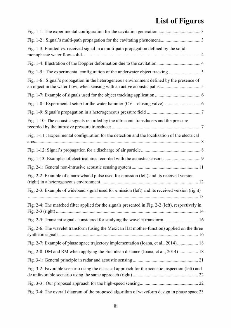
produce cavitational vortex while the flow rate increases. Fig. 1-1 presents the experimental
configuration.
3
Fig. 1-1: The experimental configuration for the cavitation generation
In this facility, the cavitation parameters, in terms of rotational vortex speed and the
density of bubbles, are controlled by the flow rate parameters. The purpose of our work,
which will be detailed further in the thesis, is to define an active acoustic non-intrusive
sensing system based on the measurement of signal’s deformations when propagating in this
dynamic diphasic environment. Actually, because of the presence of the two aggregation
states, liquid and gas, we can consider that the propagation will be done in a heterogeneous
environment, characterized by different zones with different propagation parameters. In
addition, the conic shape of the acoustic sensors contributes to the multi-path behavior of the
propagation in this environment. Another difficulty is the dynamic aspect of the configuration
while the parameters of the flow and cavitation change over the time.
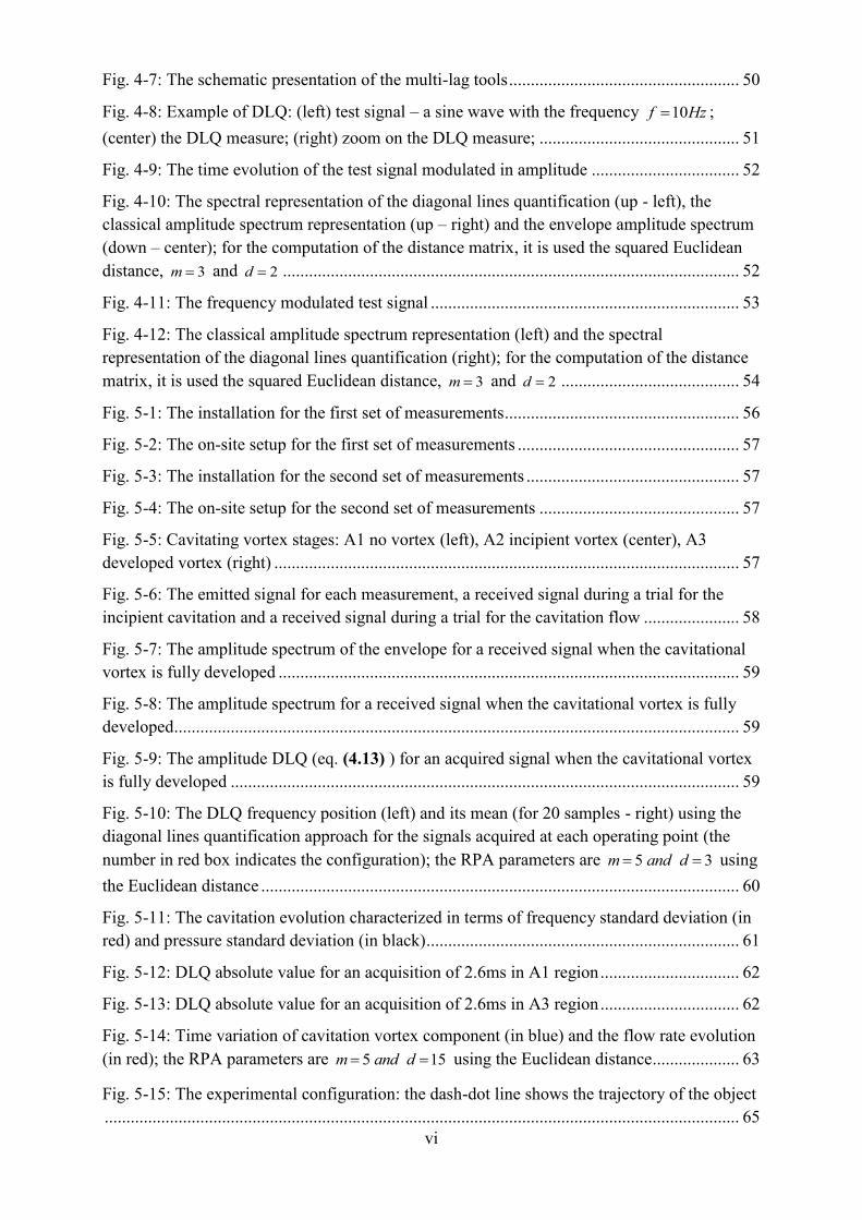
The next figure illustrates the specificity of this application described above.
Fig. 1-2 : Signal’s multi-path propagation for the cavitating phenomena
From signal’s model point of view, we can derive two special cases:
When the water is monophasic: the deformation operator kD is defined by the
attenuation and delay (Fig. 1-2 - similar to eq. (1.4)):
( ) ( )k k ks t s t D (1.5)
where k is the index of the propagation path. Therefore, the received signal is:
( ) ( ) ( )k k
k
r t s t n t (1.6)
Since the propagating paths are very close, the effect of the signal is the deformation due
to the superposition of different arrivals so that the received signal has a different duration and
a completely different amplitude shape than the emitted signal. This is illustrated in Fig. 1-3.

4
Fig. 1-3: Emitted vs. received signal in a multi-path propagation defined by the solid-monophasic water flow-
solid.
When the cavitation appears: then, the deformation operator kD is characterized by
attenuation, delay as well as the Doppler effect that acts as a deformation of the
instantaneous phase of the signal:
( ) ( ( )) exp( ( ))k k k k ks t s t t A j t D (1.7)
where ( )
( ) kk
r tt t
c
and ( )kr t is the time (Doppler) dependent position vector.
Fig. 1-4: Illustration of the Doppler deformation due to the cavitation
Fig. 1-4 illustrates the deformation of the transmitted signal in the presence of
cavitation phenomena generated in our experimental setup. As it will be discussed in the
devoted part of this thesis, this deformation is fast varying in time, while the cavitation
structure changes in time.
Underwater object tracking
The underwater object tracking is an essential task in the marine community with
uncountable number of applications – intrusion detection in protected area, underwater
mammal surveillance, fish detection, pollution monitoring, to just mention few of possible
applications (Yuan, et al., 2000).

5
The general context of this application field can be summarized by the presence of a
moving object and the definition of two active acoustic paths, as indicated in Fig. 1-5.
Fig. 1-5 : The experimental configuration of the underwater object tracking
In this case, the heterogeneity of the environment is given by the set water – object –
water (Fig. 1-6).
Fig. 1-6 : Signal’s propagation in the heterogeneous environment defined by the presence of an object in the
water flow, when sensing with an active acoustic paths
It goes that, the deformation operator is:
0( ) exp , 1,krkk k
water oil
drs t A j t k N
c c
D (1.8)
where kr is the thk water propagation path,
krd is the
thk oil propagation path and
02 b
rubber
l
c where bl is the thickness of the rubber wall of the balloon and rubberc is the
acoustic propagation velocity in rubber.
The next figure (Fig. 1-7) illustrates both transmitted and the received signal,
corresponding to an impulse emission – propagation couple.

6
Fig. 1-7: Example of signals used for the object tracking application
The purpose of this application is to find a suitable method for the detection of an
underwater object using bi-static acoustic paths and without synchronization between sensors.
Actually, in some real application, when the transmitting and the receiving sensors need to be
far, in order to cover a wider zone, the synchronization becomes an important issue, especially
in the case of immerged sensors. As we will see further, the theoretical contributions of this
thesis can be a potential solution in this context.
1.1.2. Passive configurations
Measuring pressure transient in water pipes
Pressurized pipes sometimes present unsteady flows which happen because of a
sudden hydraulic change in the system (eg. closing of a valve). Among the effects of these
changes, a commonly met phenomenon is the water hammer which usually is caused by a
suddenly closed valve (Hachem & Schleiss, 2012). Thus, the fluid changes its direction or
stops its motion. The major and dramatic effect of the water hammer phenomenon is that the
system exhibits a pressure variation which may cause from vibrations to pipe collapse (Fig.
1-8).
Fig. 1-8 : Experimental setup for the water hammer (CV – closing valve)
The heterogeneity of the environment, in this application, it is caused by the
phenomenon itself: the environment is no longer homogenous, because the pressure field is no
longer the same. Therefore, the environment is mainly characterized by the water and the

7
dynamic pressure field (Fig. 1-9). The main purpose in this application is to measure this
dynamic pressure field from the interference between the acoustic propagating wave and the
field, as illustrated in the next figure.
Fig. 1-9: Signal’s propagation in a heterogeneous pressure field
The deformation operator kD becomes:
( ) exp kk k
pressure
Ls t A j t
c
D (1.9)
where pressurec is the propagation speed of the pressure field and kL is the distance between
the CV and the ultrasonic transducers.
Fig. 1-10: The acoustic signals recorded by the ultrasonic transducers and the pressure recorded by the intrusive
pressure transducer
This application has the purpose to evaluate, using a non-intrusive method, the water
hammer effect, namely the pressure variation inside the pipeline. This can be achieved based
on an accurate estimation of the pressure field propagation speed (Houghtalen, Akan, &
Hwang, 2010) which is almost the same as the speed of the acoustic wave, Fig. 1-10.
The advantage of this approach is that the ultrasonic transceivers have just to be placed
on the pipe without requiring any extra modification of the system and without direct contact
with the fluid.

8
Electrical arcs
Another case of sensing in heterogeneous environment is the surveillance of electrical
power systems - in the presence of transient phenomena. The surveillance of photovoltaic
system in the presence of arc faults is the main application that is considered in our work.
One possible solution for the continuous surveillance of an equipment, in order to
detect in real time the generation of faults such as electrical arcs (EA), is to listen, using a
hybrid electromagnetic/acoustic array, the perimeter of interest (Fig. 1-11).
Fig. 1-11 : Experimental configuration for the detection and the localization of the electrical arcs
The particularity of this application is that, from acoustic point of view, the EA
(discharges of air particles) creates different acoustic signatures, according to the direction of
arrival with respect of each element of the acoustic array.
Fig. 1-12: Signal’s propagation for a discharge of air particle
The heterogeneity is caused by the different angles of arrival, k , at the sensing
system, Fig. 1-12. The deformation operator can be written as:
{ ( )} exp coskk k k
Ls t A j t
c
D (1.10)
Moreover, the use of the wide band antenna, namely the electromagnetic propagation
mode accentuates the heterogeneity of the propagation of the transient electrical arc to the
acoustic array (Fig. 1-13).
x y
z
S2S3S4
Electrical Arc
Photovoltaic panel
Wide band antenna

9
Fig. 1-13: Examples of electrical arcs recorded with the acoustic sensors
The applicative contexts briefly presented in this part are just few examples of
problems consisting of the estimation of physical parameters in a heterogeneous propagation
and dynamic environment. The main objective of the thesis is to propose new methods for
signal’s analysis that could provide, with respect of the state of the art, an interesting
alternative for the sensing techniques required for these applications.
1.2. Thesis outline
Chapter 2 presents a state of the art of the techniques used in acoustic sensing field,
from signal processing perspective, in a dynamic configuration. Then, we present a data-
driven analysis technique based on the phase diagram concept that constitutes an interesting
representation space for the problems we propose to solve.
Chapter 3 describes a new concept for the active sensing. The major part of this
principle is the emission which is a phase-space-based waveform that presents a unique shape
in the phase space and which can be easily translated into a signal. We start from the desired
phase-space-based waveform and then we move backwards, to the time series concept in
order to have a 1D signal which contains the desired information. This waveform design
technique presents the interest to create separable waveforms, even if they share the same
time-frequency plan. The analysis of such signals, using instantaneous frequency law tracking
in phase diagram domain, is then proposed as the processing done at the receiving level.
Chapter 4 focuses on the analysis of the signals using new descriptors defined in the
phase diagram/RPA domain. Firstly, the time-distributed recurrence measure is described and,
then, used for the detection of transient signals. Next, the multi-lag phase analysis is
introduced and applied on synthetic signals with close parameters in order to discriminate
them. Finally, the diagonal lines quantification is presented as applied on modulated signals.
Chapter 5 presents the experimental results using proposed concepts previously
presented in active configurations: the cavitating environment application is presented and the
flow evolution is characterized using the diagonal lines quantification; the underwater object
tracking is, then, presented and, with the use of the time-distributed measure, the object is
tracked.
Chapter 6 describes the water hammer application and estimates the phenomenon
parameters using the RQA descriptors. Then, the electrical arc application is presented for the

10
detection, localization and characterization of electrical faults using the phase diagram/ RPA
concepts.
Finally, the conclusion lays out a synthesis of the thesis, our main contributions and
proposes the perspectives for further research works.

11
CHAPTER 2
2. Thesis work motivation and positioning
The general context of this thesis evolves around the sensing of transient and dynamic
phenomena (Gao, et al., 2007), (Serbanescu, Cernaianu, & Ivan, 2009) such as cavitation,
pressure transient, etc. as it was discussed in the Chapter 1.
In order to define the positioning of our work in this general context, we consider as
an illustrative example, an active sensing system composed by two acoustic transducers: one
for emission and the other for reception (Fig. 2-1).
Fig. 2-1: General non-intrusive acoustic sensing system
The requirements for sensing (Emitter/Receiver) system are synthesized in Table 2-1.
Requirements Emitted waveform Received signal
processing
1. Accurate time parameter estimation
for flow velocity, object detection and
localization
Good robustness face
to the propagation
phenomena
High resolution and
robustness
2. Accurate spectral parameters Long duration signals
to integrate Doppler
effects
- High resolution n
spectral domain
- Sensing
phenomena with
weak amplitude
3. High sped sensing for dynamic (fast)
phenomena
Signals with high pulse
repetition frequency
(PRF)
Capacity of satisfying
the first and second
requirements
Table 2-1: The requirements for a general sensing system
The purpose of this system is to achieve a non-intrusive characterization of high
dynamic phenomena such as the fluid parameters (mono/biphasic). In these applications, one
of main parameters to estimate is the time of flight (TOF) which relates us to the flow velocity
(Ioana, et al., 2014), as well as the spectral information related to the speed flow profil in bi-

12
phasic configuration. Such (general) applicative context requires new signal analysis and
processing techniques. The contributions proposed by this thesis constitute a potential
interesting sensing tool.
2.1. Emission
2.1.1. Narrowband pulses
The active context of the sensing of dynamic phenomena requires a special attention
for the emission part. The received signal characterizes better the studied phenomenon if it is
well adapted to the propagation environment.
In the domain of acoustic inspection or parameters estimation the main sensing
techniques are built around the time of arrival measurements. The simplest way is to measure
the travel time between an emitted waveform and the received one. The most used transmitted
waveforms are the pulses, defined as:
0( ) exp( ), [ , ], 1,ss t A j t t kT kT T k N (2.1)
where 0 02 f , 0f is the central frequency of the transducers, T is the pulse period and
sT is the duration of the pulse.
Fig. 2-2: Example of a narrowband pulse used for emission (left) and its received version (right) in a
heterogeneous environment
The signals presented in Fig. 2-2 are recorded for an application related to the
underwater object detection. The emitted signal is a windowed narrowband signal at 1MHz
and a duration of 5 s . The configuration is static: both the water and the immersed object
are not moving. As it is shown by Fig. 2-2, the received signal is strongly deformed, because
of the heterogeneity of the environment - solid-fluid-solid.
This example illustrates the main limitation of narrow band pulses: the amplitude
deformation as well as the complex behavior of the propagation environment makes difficult
the problem of time of arrival (TOA) estimation.
As an alternative, the wideband signals can be used, starting from the fact that the
frequency information is generally more robust than the amplitude’s one.

13
2.1.2. Wideband pulses
The signals with high bandwidth-duration product are well known in radar and sonar
applications (Daniels, 1999), thanks to their robustness in complex propagation contexts. The
general definition of such signals is:
( ) exp( ( ))WBs t A j t (2.2)
where ( )WB t is the instantaneous phase of the signal. From this variable, the Instantaneous
Frequency Law (IFL) of the signal is defined as its first derivative:
( ) ( )WB WBd
t tdt
(2.3)
The instantaneous phase can be characterized using an analytical polynomial form:
0
( )N
kWB k
k
t a t
(2.4)
where ka are the coefficients of the polynomial phase. Depending on these coefficients, the
shape of the IFL can be flat ( 1k ), linear ( 2k ), cubic ( 3k ), etc.
Fig. 2-3: Example of wideband signal used for emission (left) and its received version (right)
In Fig. 2-3, we present the signals emitted and received for the same application as the
one conducting to the signal illustrated in Fig. 2-2. The emitted signal is a linear chirp from
[800 ,1200 ]kHz kHz of 10 s duration. Compared with the narrowband received signal, the
wideband received one has higher amplitude and less interference, proving its better
robustness to the propagation effects.
Still, a trade-off between the bandwidth of the signal and its duration must be
considered: a higher frequency resolution implies a longer duration of the signal which
usually leads to destructive interferences in multi-path configuration.
In order to achieve good parameters estimation capabilities in such experimental cases,
the needing for new modulation concepts is obvious. The solution proposed in this thesis is to
design different modulations, in the same time-frequency region, but with elements that will
allow their separation at the reception level. Our contribution is to design these modulations
in the phase diagram domain as we will present in the Chapter 3.

14
2.2. Reception
At the receiver level, either we are in active or passive configuration, the aim of our
analysis is to estimate the physical parameters of the received signals. Independently of the
waveform type, the received signals are strongly deformed. In order to place our contribution
with respect of the state of the art, we will briefly present the major classes of methods
traditionally used to estimate the signal’s parameters.
2.2.1. Energetic techniques
In active configurations, one of most common analysis techniques is the matched filter
(MF) method. Considering r the received signal, then the output of the matched signal is
(Van Trees, 2001):
0
( ) ( ) ( )
t
y t r h t d (2.5)
where t is the duration of the signal to be detected and h is the impulse response of the filter
which is equal to the time reversed version of the transmitted signal, s , used as reference.
Next, the output of the MF given in eq. (2.5) is compared with a threshold, and, if it is greater
than the threshold, the signal s is considered to be present or not.
Multiple communication and physical parameters measurements equipments are based
on this principle, especially for the detection part. The limitation of this method is that, in
terms of characterization, it does not succeed to highlight similar (but not identical)
deformations in the received signal since such deformations are not present in the reference
signal, Fig. 2-4.
Fig. 2-4: The matched filter applied for the signals presented in Fig. 2-2 (left), respectively in Fig. 2-3 (right)
For this reason, a deeper analysis of the received signals is necessary, using the main
techniques presented in the following part.
2.2.2. Projective techniques
The projective techniques are based on the principle of analyzing a signal using its
projection on a set of elementary functions from a dictionary which are used as reference for
the comparison with the studied signal.

15
There are various approaches for these techniques, we recall one among the most used
technique which, for an adequate dictionary, highlights signal’s time and scale evolution,
being a powerful tool for the signals’ characterization (Mallat, 1999). This is actually the
representation using time-scale analysis and, particularly, the wavelet transform analysis.
A wavelet (Mallat, 1999) is a zero average function:
( ) 0t dt
(2.6)
This function (often called mother wavelet) is dilated with the scale parameter s and
translated with the parameter u . Hereby, the orthonormal basis can be built for 2s .
,1
( )s ut u
tss
(2.7)
As an example of well-known wavelets, we mention the families of functions
presented in (Mallat, 1999), (Meyer, 1993), (Daubechies, 1992), (Daubechies, 1990), (Auger,
et al.).
Therefore, the wavelet transform of a signal ( )x t at scale s and time position u is
defined as:
*1
( , ) ( )t u
Wx u s x t dtss
(2.8)
It goes that a wavelet transform is able to quantify the time-frequency variations, but
based on the scale provided by the wavelet basis. Hereby, in order to have a good wavelet
representation, it is essential to determine an adequate mother function which resembles as
much as possible the analyzed signal, ( )x t (Mallat & Zhong, 1992).
In order to illustrate the particularities of wavelet analysis in the case of transient
signals having close features, we consider three transients with very close characteristics.
These signals are defined by this generic formula:
( , , )
sin 2 [ ] , 1,[ ]
[ ],a f b
a f n b n n Ns n
a b n otherwise
(2.9)
where 2
sfNf
and 10sf MHz is the sampling frequency.
These signals, 1 1 11( , , )a f bs ,
2 2 22( , , )a f bs , respectively 3 3 33( , , )a f bs have the following
relationships between their parameters: 1 2/ 1 / 0.6 1.66a a , 1 3/ 1 / 0.3 3.33a a ,
5 51 2/ 2 10 / 1.9 10 1.05f f , 5 5
1 3/ 2 10 / 1.6 10 1.25f f , 1 2 3b b b is an additive
white Gaussian noise and 20 , 1,3iSNR dB i . Fig. 2-5 presents the signals considered in eq.
(2.9).

16
Fig. 2-5: Transient signals considered for studying the wavelet transform
These synthetic signals seem to be quite similar, but, at a closer look, slight
differences appear. The results obtained with the wavelet analysis are shown in Fig. 2-6.
Fig. 2-6: The wavelet transform (using the Mexican Hat mother-function) applied on the three synthetic signals
It can be observed that the slight differences between the signals cannot be highlighted
by the wavelet transform: their presence is detected and located in time, but their shape does
not present any discriminating element (beside the amplitude differences).
Once again, even if the problem of detection and localization is solved (although, it
frequently requires the managing of a large dictionary), the problem of signal characterization
and discrimination between signals is present when it comes to analyze signals with close
characteristics.
2.2.3. Data-driven techniques
While the projective techniques require the definition of the elementary functions, the
interest of data-driven techniques is clear when this definition is not straightforward.
These techniques have the major advantage that they do not use any model to analyze
the data. They analyze the signal based on the organization of samples in time. One of the
current data-driven analysis techniques is based on the concept of Recurrence Plot Analysis
(RPA) which has been firstly introduced by Eckmann et al. (Eckmann, Kamphorst, & Ruelle,
1987).
This concept is based on the phase space representation and, as its name suggests, it
highlights the recurrences of trajectories from higher-dimension phase spaces. The term of
“recurrence” - one main property of conservative dynamic systems (Zbilut & Webber Jr.,

17
1992), (Webber Jr. & Zbilut, 1994), (Webber Jr. & Zbilut, 2005), (Zbilut & Webber Jr.,
2007), (Marwan, 2008), (Marwan, Schinkel, & Kurths, 2013) – means that the dynamical
system under study returns in a state previously visited. The method is quantified using
Recurrence Quantification Analysis (RQA).
The choice of the RQA based on RPA concept for the analysis of signals coming from
heterogeneous environments is based on the fact that it is a data-driven method which does
not require a priori information about the system, knowing that such information is not always
available (Zbilut & Webber Jr., 2006), (Marwan, et al., 2007).
The recurrence information is very important, offering us new insights in the evolution
of dynamic systems. In our work, we are interested of the system state changes that are not
determined by random causes, but they are the results of a nonlinear input that causes them to
change their state suddenly, exposing the system to major collapse.
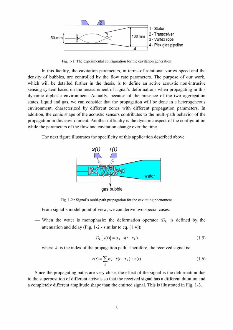
The phase diagram concept starts by considering the following time series:
[1], [2],..., [ ]x x x x N (2.10)
Then, this time series is represented in phase space. Its values become the coordinates
of the m - dimensional space and, consequently, the vector sample is:
1
[ ( 1) ] , 1,m
i k
k
v x i k d e i M
(2.11)
where m is the embedding dimension, d is the delay, ke is the unit vector of the axis that
define the phase space, ( 1)M N m d and N is the length of the time series. Usually, the
embedding dimension and the delay are chosen using the false nearest neighbor method and
the mutual information method, respectively (Marwan, et al., 2007), (Kantz & Schreiber,
1997), (Thiel, et al., 2002), (Thiel, et al., 2004).
Fig. 2-7 illustrates the phase space construction algorithm. Each point of the phase
space trajectory has as coordinates the time series values, namely signal’s samples.
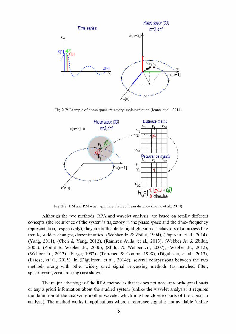
Next, the distances between the vectors in the phase space are represented on the
distance matrix (DM), eq. (2.12). When compared with a threshold, the recurrence matrix
(RM) is obtained, eq. (2.13).
, ( , )i j i jD v vD (2.12)
, ( ) ( , )i j i jR i v v D (2.13)
where ( , ) D is a distance applied on the vectors from the phase space (Euclidean distance
(Marwan, et al., 2007), (Marwan & Kurths, 2002), L1 norm (Kantz & Schreiber, 1997),
angular distance (Birleanu, et al., 2012), (Ioana, et al., 2014), scalar dot product distance
(Birleanu, et al., 2012), etc.), ( ) is the Heaviside step function and ( )i is the threshold
considered for recurrence. A graphical representation is presented in Fig. 2-8 when using the
Euclidean distance.
18
Fig. 2-7: Example of phase space trajectory implementation (Ioana, et al., 2014)
Fig. 2-8: DM and RM when applying the Euclidean distance (Ioana, et al., 2014)
Although the two methods, RPA and wavelet analysis, are based on totally different
concepts (the recurrence of the system’s trajectory in the phase space and the time- frequency
representation, respectively), they are both able to highlight similar behaviors of a process like
trends, sudden changes, discontinuities (Webber Jr. & Zbilut, 1994), (Popescu, et al., 2014),
(Yang, 2011), (Chen & Yang, 2012), (Ramirez Avila, et al., 2013), (Webber Jr. & Zbilut,
2005), (Zbilut & Webber Jr., 2006), (Zbilut & Webber Jr., 2007), (Webber Jr., 2012),
(Webber Jr., 2013), (Farge, 1992), (Torrence & Compo, 1998), (Digulescu, et al., 2013),
(Larose, et al., 2015). In (Digulescu, et al., 2014c), several comparisons between the two
methods along with other widely used signal processing methods (as matched filter,
spectrogram, zero crossing) are shown.
The major advantage of the RPA method is that it does not need any orthogonal basis
or any a priori information about the studied system (unlike the wavelet analysis: it requires
the definition of the analyzing mother wavelet which must be close to parts of the signal to
analyze). The method works in applications where a reference signal is not available (unlike

19
the matched filter method) (Digulescu, et al., 2014c), (Ioana, et al., 2014), (Digulescu, et al.,
2016c), (Le Bot, Gervaise, & Mars, 2016).
In terms of RQA, we recall the most known measures as the recurrence rate, the
determinism, the laminarity, etc. (Zbilut & Webber Jr., 1992), (Webber Jr. & Zbilut, 1994),
(Webber Jr. & Zbilut, 2005), (Webber Jr., 2012), (Webber Jr., 2013), (Zbilut & Webber Jr.,
2006), (Zbilut & Webber Jr., 2007) which measures the states of the system based on the RM.
2.3. Chapter summary
This chapter shortly presents the existing methods for the analysis of transient signals
in terms of detection and characterization.
These methods present many advantages, but they also have limitations. In the next
chapters, we present our approach based on the concept of phase diagram and the RQA based
on the RPA method. For the active sensing part, we propose the use of phase space-based
adaptive waveforms which are better suited for the propagation phenomena specific to the
sensing of transient signals. The passive sensing part presents a new approach for the analysis
and characterization of transient signals based on the concept of RQA.


21
CHAPTER 3
3. Active sensing: phase diagram-based adaptive waveform
3.1. Introduction
The active sensing techniques are the heart of any system aimed to analyze physical
parameters of an environment of interest, either by acoustic or electromagnetic waves. The
sensing signal is always designed according to the application specificities: propagation
phenomena, objects to detect, parameters to sense, etc. This is always the case in sonar/ radar
domains, where the transmitted signal’s parameters are chosen from physical considerations:
the central frequency and the bandwidth are chosen to minimize the wave attenuation
effect as well as to best fit to the sensors characteristics
the signal’s duration is chosen to meet the required resolution
Another parameter of great importance is the PRF (Pulse Repetition Frequency) which
is related to the maximum range of sensed region. The classical approach considers the
principle presented in Fig. 3-1.
Fig. 3-1: General principle in radar and acoustic sensing
From this perspective, the environment inspection is done by respecting the relation
between the maximum distance and the PRF.
Still, for sudden phenomena or fast changes, this approach could skip them, the PRF
being too small to detect these transient phenomena. An example is presented in Fig. 3-2.

22
Fig. 3-2: Favorable scenario using the classical approach for the acoustic inspection (left) and de unfavorable
scenario using the same approach (right)
In the first case (Fig. 3-2, left), the detection of the object passing in front of the
sensors is done from the reflected wave, the range being calculated as a product between the
wave velocity and the half of time of flight. With this technique, the characterization of the
object is almost impossible as illustrated in the Fig. 3-2 (right). Two different objects are
traduced, at the receiving sensor, by more or less similar reflected waves, making difficult
their identification.
One solution is then to increase the PRF in order to allow a high speed sensing, as it is
illustrated in Fig. 3-3.
Fig. 3-3 : Our proposed approach for the high-speed sensing
These signals contain some unique information that allow us to increase the PRF
disregarding the classical condition, in order to monitor the environment at higher sensing
speed. The main difficulty is to add a unique identifier knowing that the amplitude or phase
changes could interfere, from one emitted pulse to another, making difficult their separation at
the receiving point. The appropriate design of the transmitted pulses is then the main objective
of our contribution, presented in the next section.

23
3.2. Phase diagram-based waveform design
One way to generate separable pulses is to design them in diagram phase, in different
regions which bring them “orthogonal” in this representation space.
Fig. 3-4 presents the overall diagram of the algorithm.
Fig. 3-4: The overall diagram of the proposed algorithm of waveform design in phase space
3.3. Emission
The starting point is the idea to design a pattern in the phase space which has a unique
evolution and, afterwards, to translate it in a 1D signal into a one-to-one correspondence.
Step 1: we represent a lobe in a 3D phase diagram space. The core of this idea is
suggested by the trajectory of a transient signal in phase space (Candel, et al., 2012a),
(Candel, et al., 2012b).
Hereby, the simplest way to represent the waveform’s trajectory in shape of a lobe is
to compose it of two director vectors, as in Fig. 3-5:
, {1,2}, , , 0
( , , )
n n n n n n n
n n n n
v a i b j c k n a b c
v a b c
(3.1)
Step 1: desired lobe
in the phase space
Step 2: get the 1D
signal which
contains this lobe
Step 3: Recover the
lobe information
from the signal
24
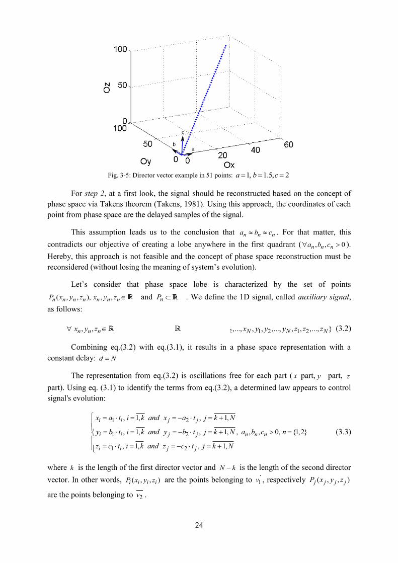
Fig. 3-5: Director vector example in 51 points: 1, 1.5, 2a b c
For step 2, at a first look, the signal should be reconstructed based on the concept of
phase space via Takens theorem (Takens, 1981). Using this approach, the coordinates of each
point from phase space are the delayed samples of the signal.
This assumption leads us to the conclusion that n n na b c . For that matter, this
contradicts our objective of creating a lobe anywhere in the first quadrant ( , , 0n n na b c ).
Hereby, this approach is not feasible and the concept of phase space reconstruction must be
reconsidered (without losing the meaning of system’s evolution).
Let’s consider that phase space lobe is characterized by the set of points
( , , ), , ,n n n n n n nP x y z x y z and 3nP . We define the 1D signal, called auxiliary signal,
as follows:
31 2 1 2 1 2, , , ( , , ) { , ,..., , , ,..., , , ,..., }auxn n n n n n n N N Nx y z P x y z x x x y y y z z z (3.2)
Combining eq.(3.2) with eq.(3.1), it results in a phase space representation with a
constant delay: d N
The representation from eq.(3.2) is oscillations free for each part ( x part, y part, z
part). Using eq. (3.1) to identify the terms from eq.(3.2), a determined law appears to control
signal's evolution:
1 2
1 2
1 2
, 1, , 1,
, 1, , 1, , , , 0, {1,2}
, 1, , 1,
i i j j
i i j j n n n
i i j j
x a t i k and x a t j k N
y b t i k and y b t j k N a b c n
z c t i k and z c t j k N
(3.3)
where k is the length of the first director vector and N k is the length of the second director
vector. In other words, ( , , )i i i iP x y z are the points belonging to 1v , respectively ( , , )j j j jP x y z
are the points belonging to 2v .

25
We recall that in step 1, it was imposed that , , 0, {1,2}n n na b c n . Still, in eq. (3.3),
the coordinates belonging to 2v appear to have negative coefficients. This is caused by two
conditions that our lobe has to meet:
The lobe must return to its original starting point
The signal belongs to a continuous measurement. Therefore, we must accomplish the
sampling condition: it and jt are, in fact, the sampling moments of the signal with the
sampling period sT .
0
0
0
( 1) , 1,
( 1) , 1,
[ ( 1) ] ( )
i s
j s
s s
t t i T i k
t t j T j k N
t k T j k T
(3.4)
Based on the observations presented above, in Fig. 3-6, we illustrate such signal.
Fig. 3-6: The auxiliary signal aux with the following parameters: 1 1 11.5, 1.1, 1.9a b c ,
2 2 21.5, 1.2, 1.8a b c , 50, 100, 5sk N f MHz and 0 1/ s st f T
Considering that ( , , ), , ,n n n n n n nP x y z x y z is the evolution of the aux signal in the
phase space, its trajectory is easily obtained (Fig. 3-7).
Fig. 3-7: The phase space lobe obtained using the signal aux from Fig. 3-6

26
The phase space lobe is obtained using the eq. (3.1), but it presents two limitations:
the lobe is too tight, making this representation sensitive even to low levels of noise
the corresponding signal of this phase space lobe presents discontinuities/ breaks in its
evolution when the coefficient changes; in Fig. 3-6, 1 2a a , the signal is continuous, but
1 2b b and 1 2c c , the signal is discontinuous when the coefficient changes (the effect is
highlighted by the red circles)
In order to obtain a larger lobe, we impose different number of points for the two
director vectors that create the phase space, so, the eq. (3.3) becomes:
1 1 2 1
1 2 2 2
1 3 2 3
, 1, , 1,
, 1, , 1, , , , 0, {1,2}
, 1, , 1,
i i j j
i i j j n n n
i i j j
x a t i n and x a t j n N
y b t i n and y b t j n N a b c n
z c t i n and z c t j n N
(3.5)
The discontinuity issue of the aux signal corresponding to the phase space lobe is
solved by imposing the continuity condition for the descending slopes from the aux signal.
1 1 2 1
1 2 2 2
1 3 2 3
[ ] [ 1]
[ ] [ 1]
[ ] [ 1]
x n x n
y n y n
z n z n
(3.6)
In fact, the slopes of the lines from the aux signal are the coefficients of 2v . Using
the continuity condition, eq. (3.6) and considering that the lobe returns to its original point,
meaning that 1 2 1 2 1 2[1] [ ] 0, [1] [ ] 0, [1] [ ] 0x x N y y N z z N , it results in a relationship
between the two director vectors:
2 1 1 1
2 1 2 2
2 1 3 3
/
/
/
a a n N n
b b n N n
c c n N n
(3.7)
Fig. 3-8: The phase space lobe and its corresponding aux signal based on eq. (3.5) and (3.7) with the following
parameters: 1 1 1 1 2 3100, 1, 1.2, 1.3, 50, 50, 60N a b c n n n

27
Fig. 3-9: The phase space lobe and its corresponding aux signal based on eq. (3.5) and (3.7) with the
following parameters: 1 1 1 1 2 3100, 1, 1.2, 1.3, 40, 50, 60N a b c n n n
From Fig. 3-8 and Fig. 3-9, it can be observed that the parameters 1 2 3,n n and n
reshape the phase space lobe such that it becomes larger and: it contains an extra vector (line)
when two of them are equal (Fig. 3-8), or it contains two extra vectors (lines) when all three
of them are different (Fig. 3-9).
3.4. Reception
Step 3: Recover the lobe information from the signal
Our first attempt was to transmit the phase space lobe into an amplitude modulation.
Therefore, we define two auxiliary signals with the following parameters that are translated in
amplitude modulations, Fig. 3-10:
1 1 11
1 2 3
1 1 12
1 2 3
1, 1.5, 2:
400, 500, 600, 1000
2, 1, 1.4:
400, 500, 600, 1000
a b caux
n n n N
a b caux
n n n N
(3.8)
Fig. 3-10: The amplitude modulated signals (left) which have as envelope the auxiliary signal defined in eq. (3.8)
shown in phase space representation (right)

28
At reception, the information held in signal’s envelope is extracted in conditions free
of noise and at different signal-to noise ratios (SNR), Fig. 3-11.
Fig. 3-11: The recovered signal’s envelopes (normalized values) for: SNR and 20SNR dB (left);
SNR and 15SNR dB (right);
Although the new representation space provides a new perspective in terms of
adaptive waveform for active configurations, the modulation amplitude approach does not
offer reliable results in real propagation conditions. It is obvious that even at 20 dB is hard to
distinguish between the two lobes. Therefore, the alternative way is to introduce the lobe
information in the frequency's evolution
Firstly, the frequency range must be established. In this new interpretation of phase
diagram trajectories, the coefficients 1 1 1,a b and c become the maximum frequencies that the
signals reach in time. In other words, as the auxiliary signals (that create the phase space
lobes) contain only straight lines which vary in time, the modulated signal will contain just
linear frequency modulations (LFM) that follow the trend given by the auxiliary signals.
Hereby, these signals become from now the IFLs of the signals.
After defining the IFLs using the same algorithm as shown in eq. (3.5) and (3.7), this
set is composed of LFMs which vary in the same time-frequency region in different manners,
but their trajectory in phase space is UNIQUELY identifiable..
As an example, we consider a central frequency of 1 MHz and in the range of
[800 , 1200 ]kHz kHz . We define the auxiliary signals where the coefficients 1 1 1,a b and c
correspond to the frequency parameters.
6 6 61 1 1
11 2 3
6 6 61 1 1
21 2 3
1 10 , 1 10 , 1.2 10:
0.4 , 0.5 , 0.6 , 1000
1.2 10 , 1 10 , 1 10:
0.4 , 0.5 , 0.6 , 1000
a b caux
n N n N n N N
a b caux
n N n N n N N
(3.9)
The modulated signals with the IFLs defined in eq. (3.9) are presented in Fig. 3-12, as
well as their spectrogram representation, Fig. 3-13.
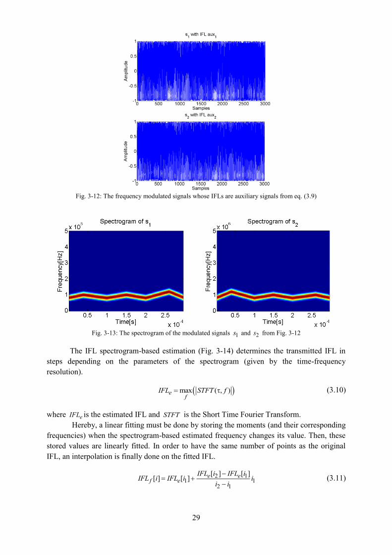
29
Fig. 3-12: The frequency modulated signals whose IFLs are auxiliary signals from eq. (3.9)
Fig. 3-13: The spectrogram of the modulated signals 1s and 2s from Fig. 3-12
The IFL spectrogram-based estimation (Fig. 3-14) determines the transmitted IFL in
steps depending on the parameters of the spectrogram (given by the time-frequency
resolution).
max ( , )ef
IFL STFT f (3.10)
where eIFL is the estimated IFL and STFT is the Short Time Fourier Transform.
Hereby, a linear fitting must be done by storing the moments (and their corresponding
frequencies) when the spectrogram-based estimated frequency changes its value. Then, these
stored values are linearly fitted. In order to have the same number of points as the original
IFL, an interpolation is finally done on the fitted IFL.
2 11 1
2 1
[ ] [ ][ ] [ ] e e
f eIFL i IFL i
IFL i IFL i ii i
(3.11)

30
where fIFL is the fitted IFL and eIFL is the spectrogram estimated IFL (eq. (3.10)) where 1i
and 2i are the time bins where the value of eIFL changes.
Fig. 3-14: The extracted IFLs using the spectrogram for the modulated signals 1s (left) and 2s (right)
In Fig. 3-15, the fitted IFL and the original IFL are plotted in the phase space.
Fig. 3-15: The phase space lobes provided by the IFLs from 1s and 2s
As shown in Fig. 3-15, the IFL shape is preserved in the phase space domain.
Moreover, the phase space provides a new representation space for the discrimination of these
signals.
This new waveform design concept has a great advantage in terms of separation of
signals. In time and frequency domain, the new modulations are not separable (Fig. 3-16) as it
is shown by their correlation and spectrum.

31
Fig. 3-16: The correlation of the modulated signals 1s and 2s (left) and their amplitude spectrum (right)
Obviously, the auxiliary signals also cannot be discriminated from time/frequency
domain, Fig. 3-17.
Fig. 3-17: The correlation of the auxiliary signals 1aux and 2aux (left) and their amplitude spectrum (right)
The capacity of phase diagram to encode separable signals is then used in order to
generate multiple separable signals, that are overlap in time and in frequency but still
separable in the phase diagram domain.
As an illustrative example, let us consider the following auxiliary signals:
6 6 61 1 1
11 2 3
6 6 61 1 1
21 2 3
6 6 61 1 1
31 2 3
1 10 , 1.1 10 , 1.2 10:
0.5 , 0.4 , 0.6 , 500
1.1 10 , 1.2 10 , 1 10:
0.5 , 0.4 , 0.6 , 500
1.2 10 , 1 10 , 1.1 10:
0.5 , 0.4 , 0.6 , 5
a b caux
n N n N n N N
a b caux
n N n N n N N
a b caux
n N n N n N N
00
(3.12)
Next, we study the frequency modulated signal’s robustness to noise in terms of phase
space lobe representation. From Fig. 3-18 and Fig. 3-19, it can be noticed that this approach is
robust enough for a SNR of at least 10 dB.

32
Fig. 3-18: Phase space lobes in noise-free conditions: original IFL (triangles) and the spectrogram recovered IFL
(stars)
Fig. 3-19: Phase space lobes for SNR = 10 dB: original IFL (triangles) and the spectrogram recovered IFL (stars)
For SNRs below 10dB, there is a real problem with the choice of the parameters of the
spectrogram that will conduct to satisfactory results. These parameters refer especially to the
number of points for the Fourier transform computation and the overlapping of the windows.
For example, for the noise-free case, the number of points is 512, whereas for the SNR = 10
dB, the number of points is 4096, these two setting conducting to similar quality of IFL
estimate. Another limitation is the choice of these parameters which is done by several trials
that are time consuming.
Considering more than 3 lobes in the phase space, we define them as all possible
combinations of the coefficients 6 6 61 1 10.87 10 , 1 10 , 1.13 10a b c . Hereby, we get a set of
six signals, Fig. 3-20. The number of points are the same for the entire set:
1 2 30.5 , 0.4 , 0.6 , 500n N n N n N N .

33
Fig. 3-20: Phase space lobes generated from the set of 6 auxiliary signals used IFLs
Next, these IFLs are used to modulate the transmitting signal. Fig. 3-21 presents the
results of the phase space representation of the IFLs in the noise-free case.
Fig. 3-21: The original IFLs (continuous line) and the spectrogram-based recovered IFLs (stars) – noise -free
case
On the other hand, when white additive Gaussian noise corrupts the signal, the
recovered signal is not very smooth. The results are presented in Fig. 3-22 where we reinforce
that they are obtained for higher number of FFT (Fast Fourier Transform) points for the
spectrogram (compared with the case of no noise (512 points), the number of points is eight
times higher (4096 points)).

34
Fig. 3-22: The original IFLs (continuous line) and the spectrogram-based recovered IFLs (stars) for SNR = 10
dB
At lower SNRs (below 10 dB), the things become more complicated and it is difficult
to separate the signals in the phase space, Fig. 3-23.
Fig. 3-23: The original IFLs (continuous line) and the spectrogram-based recovered IFLs (stars) for SNR = 5 dB
To improve the robustness to noise and to overcome the limitation of parameter
dependence for the IFL’s spectrogram-based estimation, we need to define a new approach
for the IFLs estimation.
3.2.1. Phase space-based IFL estimation
In this section we introduce a new technique for IFL estimation using the phase space
representation. This approach is, once again, suggested by the evolution of a signal – sine
wave – in phase space.
Considering a sine wave of frequency 0f and sampling frequency sf , then, for a
duration D , where 0/D m f and m is a positive integer, the sine wave contains s sN D f
samples.
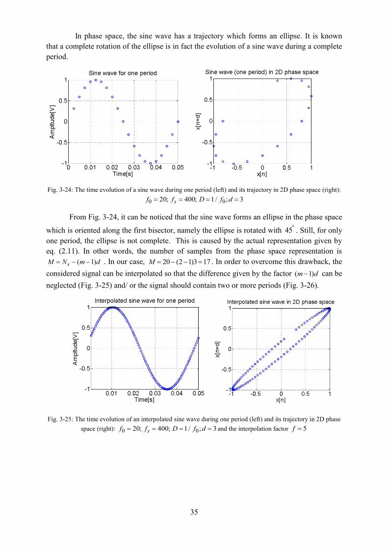
35
In phase space, the sine wave has a trajectory which forms an ellipse. It is known
that a complete rotation of the ellipse is in fact the evolution of a sine wave during a complete
period.
Fig. 3-24: The time evolution of a sine wave during one period (left) and its trajectory in 2D phase space (right):
0 020; 400; 1 / ; 3sf f D f d
From Fig. 3-24, it can be noticed that the sine wave forms an ellipse in the phase space
which is oriented along the first bisector, namely the ellipse is rotated with 45 . Still, for only
one period, the ellipse is not complete. This is caused by the actual representation given by
eq. (2.11). In other words, the number of samples from the phase space representation is
( 1)sM N m d . In our case, 20 (2 1)3 17M . In order to overcome this drawback, the
considered signal can be interpolated so that the difference given by the factor ( 1)m d can be
neglected (Fig. 3-25) and/ or the signal should contain two or more periods (Fig. 3-26).
Fig. 3-25: The time evolution of an interpolated sine wave during one period (left) and its trajectory in 2D phase
space (right): 0 020; 400; 1 / ; 3sf f D f d and the interpolation factor 5f

36
Fig. 3-26: The time evolution of a sine wave during two periods (left) and its trajectory in 2D phase space
(right): 0 020; 400; 2 / ; 3sf f D f d
Based on the observations presented above, for the phase space based IFL estimation,
we have established the following algorithm:
The trajectory of the analyzed signal is computed in 2D phase space (so that the factor
( 1)m d is minimized); previously, the signal can eventually be interpolated with an
interpolation factor f
The phase space is translated in the positive quadrant
The polar angle of each point of phase space is computed as follows:
[ ]
[ ] arctan[ ]
x n dn
x n
(3.13)
Knowing that the trajectory evolves along the first bisector, we eliminate this bias of
45 by subtracting this value from all polar angles
Next, the ellipse’s evolution is quantified: a counter is started when the first point with
a positive polar angle is found and the counter is stopped when the trajectory returns in
the same region (the angle passes from negative into positive). With the number of
points counted in this interval, 0n , we obtain the first 0f estimation, where
0 0/sf f n . The algorithm continues until the last point of the phase space is reached.

37
Fig. 3-27: The original IFL (in blue) and the phase space-based IFL estimation (in red – 5, 10f d )
For the signals presented in Fig. 3-27, we present the IFL estimation based on the
phase space evolution.
Still, the choice of the delay d must be discussed. The optimal delay depends on the
signal’s characteristics; therefore, we propose the use of the multi-lag phase analysis (MLPA)
(Bernard, et al., 2016), (Digulescu, et al., 2016c), (Bernard, et al., 2014) for the IFL
estimation. Besides the algorithm presented above, we also vary the delay and we choose the
delay that gives the IFL estimate that is the closest to the transmitted signal. This decision is
made by minimizing the cost function given by eq. (3.14).
( ) ( )o eC d IFL IFL d (3.14)
where oIFL is the original IFL and eIFL is the phase space-based IFL.
Next, a comparison between the use of a fixed delay and the MPLA is presented.
Fig. 3-28: The phase space-based IFL for 5d and SNR (left) and the MLPA phase space-based IFL
15 1 5 1 3 1 4 1 5 1 5d (according to the colors: clockwise from blue to green) and SNR (right);
continuous line – original IFL; starred line – estimated IFL
From Fig. 3-28, it goes that the IFL information do not depend on the delay when the
signal does not contain any noise.

38
Fig. 3-29: The phase space-based IFL for 5d and 5SNR dB (left) and the MLPA phase space-based IFL
21 27 1 9 30 21 25d (according to the colors: clockwise from blue to green) and 5SNR dB (right);
continuous line – original IFL; starred line – estimated IFL
When it comes to noisy signals, in Fig. 3-29, the 5SNR dB , a fixed delay does not
succeed to track the IFL, (here 5d is just an example). Using the MLPA, it is obvious that
the IFL is tracked, the optimal values of the delay varying from a signal to another.
Furthermore, although the estimated IFLs suffer a slight rotation from the original
ones, the tracking of the IFL is successfully achieved, the signals being separated and
distinguishable.
3.2.2. “Marked” lobes
This new waveform generation technique is based on the information coding via a
frequency modulation defined by the lobes designed in the phase space. If the signals defined
from these lobes are used in a time-of-flight measurement application, we propose to
introduce a special mark that will help us measuring the time of flight as the distance, in time,
between these marks are observed in the phase space.
Hereby, the two director vectors that define the lobe in the Cartesian system will
present an extra point to mark the signature of the lobe, as presented in Fig. 3-30.
Fig. 3-30: The ideal phase space representation of the “marked” lobe (auxiliary signal)
From figure above, it can be observed that the “signature” of the lobe is given by the
point 2 2 2 2( , , )P x y z in the phase space. Based on this “signature”, we aim to determine the
TOF (Fig. 3-31). The interest of this approach is that, even if the IFLs between transmitter and
the receiver are not the same (due to propagation effect or event estimation error), if the marks
are still visible, they allow a more accurate estimation of TOF than looking in time domain.

39
Fig. 3-31: The phase diagram space approach versus classical approach; in the phase diagram, the estimation of
TOF is done using the distance between the marks of emitted and received signals, respectively
The first condition which we imposed is: the four points 1 2, ,O P P and 3P should be
coplanar. It goes that:
0 0 0
1 1 1
2 2 2
3 3 3
1
10
1
1
x y z
x y z
x y z
x y z
(3.15)
Considering 0 0 0 0x y z , eq. (3.15) is equivalent to:
1 1 1
2 2 2
3 3 3
0
x y z
x y z
x y z
(3.16)
It is obvious that the points 1 2,P P and 3P should be different, therefore the lines of the
determinant from eq. (3.16) must be different. In order to accomplish the condition of
coplanarity for whatever points P1, P2 and P3, at least two columns of the determinant should
be proportional. Therefore, the coplanarity condition (eq.(3.15)) restraints to the second
condition:
, {1,2,3}, (1,2)i
i
xr i r
z (3.17)
Then, the second column is defined as: 1 3 2 2 3 1,y x y x and y x . With this condition,
the phase space representation forms a lobe with a “signature” provided that
1 2 3 2x x and x x .
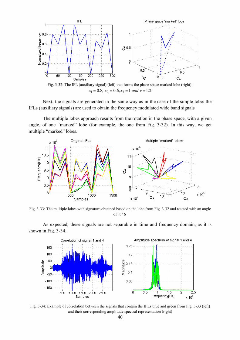
40
Fig. 3-32: The IFL (auxiliary signal) (left) that forms the phase space marked lobe (right):
1 2 30.8, 0.6, 1 1.2x x x and r
Next, the signals are generated in the same way as in the case of the simple lobe: the
IFLs (auxiliary signals) are used to obtain the frequency modulated wide band signals
The multiple lobes approach results from the rotation in the phase space, with a given
angle, of one “marked” lobe (for example, the one from Fig. 3-32). In this way, we get
multiple “marked” lobes.
Fig. 3-33: The multiple lobes with signature obtained based on the lobe from Fig. 3-32 and rotated with an angle
of / 6
As expected, these signals are not separable in time and frequency domain, as it is
shown in Fig. 3-34.
Fig. 3-34: Example of correlation between the signals that contain the IFLs blue and green from Fig. 3-33 (left)
and their corresponding amplitude spectral representation (right)

41
Next, we study the robustness to noise of the multiple “marked” lobes.
Fig. 3-35: The original IFLs (continuous line) and the phase space-based estimated IFLs (starred lines) for
20SNR dB (left) and their corresponding phase space lobes (right)
From Fig. 3-35, it can be noticed that the signals are discriminated in the phase space
for a high SNR. Although, the recovered IFLs form a larger lobe in the phase space, than the
original one, they do not overlap and present the approximately the same evolution.
Fig. 3-36: The original IFLs (continuous line) and the phase space-based estimated IFLs (starred lines) for
7SNR dB (left) and their corresponding phase space lobes (right)
The limit of the SNR is around 7dB , Fig. 3-36, in order that the lobes remain
distinguishable in the phase space and without overlapping. We mention that the phase space-
based IFL estimation is done using the MLPA and an interpolation factor of 10.
3.3. Chapter summary
This chapter illustrates a new concept for the waveform design, namely the phase
space-based waveform generation, which can be used to create a set of orthogonal signals in
phase space. This signal is created in the phase space and then its information is translated
into 1D signal. Then, there is also presented a new IFL estimation method for the signal
recovery, designed in the phase space.
These signals are tested and their feasibility is validated in our experimental setup
presented in Chapter 5.

42

43
CHAPTER 4
4. Passive sensing based on the RQA concept
Contrarily of the applications requiring an active sensing, there are a large number of
applications where active sensing is useless. This is particularly the case of the application
where the phenomena under study generate signals whose analysis allows us to understand
(detection, classification, localization, etc.) them. Currently, a special attention is carried to
the transient phenomena, characterized by very fast variation in time and frequency. The
development of new analysis methods for such signals is a current work direction in the field
of signal processing.
In this context, this chapter presents new methods for the detection, localization and
characterization of transient signals based on the concept of RQA. As discussed in chapter 2,
the RPA and RQA methods are the main approaches derived from the phase diagram and the
information that could be retrieved from this analysis can bring a deeper understanding of the
studied phenomena (Bernard, et al., 2016), (Marwan, Schinkel, & Kurts, 2013), (Webber Jr.
& Zbilut, 2005), (Zbilut & Webber Jr., 2007).
Firstly, there is highlighted the measure used for the detection and localization of a
transient signal, namely the time-distributed recurrence (TDR) measure. This measure
exploits the fact that a sudden change in the signal under study is represented as a new state in
the phase space which evolves in a totally different region than the rest of the signal’s states.
The initial idea has been presented in (Marwan, et al., 2007) and our contribution was to adapt
this idea to the problem of detection of transient sources.
Then, the multi-lag phase-space analysis will be introduced. This concept is very
useful for the characterization of transient signals (Bernard, et al., 2016), (Bernard, et al.,
2014), (Digulescu, et al., 2016c). This approach allows us to discriminate between signals
with close parameters based on their evolution in the phase diagram.
Finally, the diagonal lines quantification is presented. This approach is based on the
fact that the diagonal lines from the distance/ recurrence matrix spectral content of any signal
(Ioana, et al., 2014). With this property, we are able to highlight slight changes that appear in
signal’s spectral content, much weaker than the fundamental frequency, for instance.
4.1. Time-distributed recurrence
The core of the time-distributed recurrence (TDR) measure starts from the idea that a
sudden change in a time series represents a new state of the dynamical system (Ioana, et al.,
2014), (Birleanu, et al., 2012), (Marwan & Kurths, 2002), (Webber Jr. & Zbilut, 2005),
(Webber Jr., 2012), (Zbilut & Webber Jr., 2007), (Ramirez Avila, et al., 2013), (Yang, 2011),
(Digulescu, et al., 2016c), (Le Bot, Gervaise, & Mars, 2016). Namely, there is no recurrence

44
with the previous states. Therefore, when an appropriate distance is used, the distance/
recurrence matrix presents a horizontal/ vertical band with much fewer recurrences. When the
sum of the lines/ columns of the recurrence matrix is computed, we actually obtain the
column average (Digulescu, et al., 2016c), (Ioana, et al., 2014), which, in the case of transient
signals, significantly changes.
The TDR measure is defined as:
,
1
1[ ]
M
i n
i
TDR n RM
(4.1)
where ,i nR is the RM from eq. (2.13).
This measure can be interpreted as the column average recurrence of a given point i
or the recurrence density heterogeneity in the point i . Hereby, a solitary position of a phase
space vector changes significantly its average recurrence and it can be highlighted through the
use of the complementary version of the TDR measure from eq. (4.1):
* [ ][ ] 1
max{ [ ]}
TDR nTDR n
TDR n (4.2)
Fig. 4-1 highlights the detection based on the *TDR measure.
Fig. 4-1: The transient detection using the *TDR measure: (up) the analyzed transient signal; (left-down) the
recurrence matrix of the analyzed signal; (right-down) the analyzed signal and its TDR* based detection curve
Moreover, in order to detect only the transient signal from the analyzed observation,
the SNR must be computed. We computed it as follows: the last part of the acquired signal
(when no transient occurs) is considered as noise, [ ]z i , (unwanted signal recording

45
environmental noise), whereas the part that has a different behavior is considered as the
interest signal, [ ]s i . Both parts of the signal, [ ]s i and [ ]z i have the same length, N . Then, the
SNR is computed as:
2 210
1 1
10log ( [ ]) ( [ ])
N N
i i
SNR s i z i
(4.3)
Accordingly, the threshold of the recurrence matrix is chosen so that it includes a
percentage, , of the maximum value of the equivalent noise which has the same power as
the interest signal:
max [ ]SNR z i (4.4)
where is a constant that is chosen to nonlinearly filter the noise. In our applications,
varies from 0.4 to 0.95 .
Considering the eq.(4.4), the components of the noise (undesired parts of the signal)
are considered as recurrences; therefore, the transient signal (useful part of the signal) is
highlighted by the proposed measure.
Fig. 4-2: Transient signal detection using the TDR measure for a transition of only 11 samples where 3m ,
2d and 0.8

46
Fig. 4-2 emphasizes the advantage brought by the TDR measure, namely that the
detection provided by the detection curve is more robust. In the examples above, the detection
curve exhibits a SNR improvement of 30 dB .
The major advantage of this method is that, in applications where the SNR level of the
acquired signal varies a lot, the TDR detection curve approach improves the SNR level after
filtering the acquired signal with the detection curve. Through this approach, the signal's
power after filtering is significantly increased (in our applications, at least 10 dB), which is
very helpful for the classification and a further characterization.
4.2. Multi-lag phase-space analysis
The RPA method stands, as its name suggests it, on the concept of recurrences. Still, it
is worth to pay more attention to the phase-space representation, in order to achieve richer
characterization of signals with close parameters coming from the same source and having the
same propagation and acquisition conditions.
The phase-space representation is very rich in information regarding the evolution of a
dynamical system (Eckmann, Kamphorst, & Ruelle, 1987), (Kantz & Schreiber, 1997),
therefore the analysis can be made in any dimension, but our approach restrains, for simplicity
seeking, to a bi-dimensional representation.
Therefore, considering the Cartesian coordinate system, the phase-space representation
is defined by plotting ( , )n nx y defined as:
[ ]
[ ]
n
n
x s n
y s n d
(4.5)
where n is the thn sample of the recorded time series. It goes that eq. (2.11) can be rewritten
as: [ ] [ ]nv s n i s n d j .
Firstly, the main attributes of this representation are recalled. Considering three signals
1 2,s s and 3s defined as:
1
2
3
[ ] [ ]
[ ] [ ]
[ ] [ ]
s n s n
s n s n
s n s n
(4.6)
where , and are constant which modify the signal s through translation in time, scale
and/or amplitude, the phase-space points present the following attributes (Marwan, et al.,
2013), (Birleanu, et al., 2011):
1[ ] [ ]
2[ ] [ ]
3[ ] [ ]
i i
i i
i i
v v
v v
v v
(4.7)

47
The phase-space trajectory is invariant to translation and it points out the scale and
amplitude change. In order to introduce the concept of multi-lag phase-space analysis, we
recall the three transient signals with close characteristics given by eq. (2.9). These signals are
given by the generic signal:
( , , )
(sin[2 ] [ ]), {1,2,..., }[ ]
[ ],a f b
a f n b n n Ns n
a b n otherwise
(4.8)
where 2
sfNf
and 10sf MHz is the sampling frequency.
The considered signals 1 1 11( , , )a f bs ,
2 2 22( , , )a f bs and 3 3 33( , , )a f bs , presented in Fig. 4-3,
have the following relationships between their parameters: 1 2/ 1 / 0.6 1.66a a ,
1 3/ 1 / 0.3 3.33a a , 5 51 2/ (2 10 ) / (1.9 10 ) 1.05f f , 5 5
1 3/ (2 10 ) / (1.6 10 ) 1.25f f ,
1 2 3b b b and 20 ,iSNR dB {1,2,3}i .
Fig. 4-3: Transient signals considered for the multi-lag phase space analysis
In order to distinguish between the synthetic transient signals considered in eq. (4.8),
the multi-lag phase space analysis is considered (Digulescu, et al., 2016c), (Bernard, et al.,
2016), (Bernard, et al., 2014). The study of the representation of the trajectory for multiple
lags is done by two approaches: the elliptic modeling of the trajectory for the area estimation
in the phase-space, respectively, the polar coordinate representation.
The elliptic modeling supposes to determine the ellipse that circumscribes the phase-
space trajectory and, therefore, to estimate the area of the trajectory through the ellipse's area
computation. The area of the modeling ellipse is a new descriptor of the transient signal.
The trajectory is modeled by considering the solution that minimizes the following
system (Bernard, et al., 2016), (Bernard, et al., 2014), (Digulescu, et al., 2016c):
2
1
( , )
M
i i
i
S F x y
(4.9)
where 2 2( , ) 1F x y x y . The least mean square estimation of eq. (4.9) determines the
couple , . It goes that the major semi axes 1/a and the minor semi axes 1/b .

48
The next step after the elliptic modeling is the area estimation and the determination of
the optimal delay. The delay is considered to be optimal for the value that provides an average
value of the area.
For example, in Fig. 4-4, we present this aspect for the synthetic transient signal
shown in Fig. 4-1 (up).
Fig. 4-4: The phase space trajectory evolution using different delays
This average value area ensures a suitable phase-space representation where the
trajectory does not evolve too close to the main diagonal (case of redundancy) or its evolution
is too complicated (case of irrelevance) (Casdagli, et al., 1991).
Fig. 4-5: The evolution of the area according to the lag (delay): for the signals presented in Fig. 2-5 (left) and for
the normalized signals (right)
From Fig. 4-5, it can be noticed that the area of the signals has a similar trend with
some differences for the normalized signals. Hereby, considering the average value of the
area, 3A , the optimal delay for 1s is 1 5d , for 2s , 2 5d and for 3s , 3 6d .
With the chosen lags, the next step is to plot the phase-space trajectory into polar
coordinates:
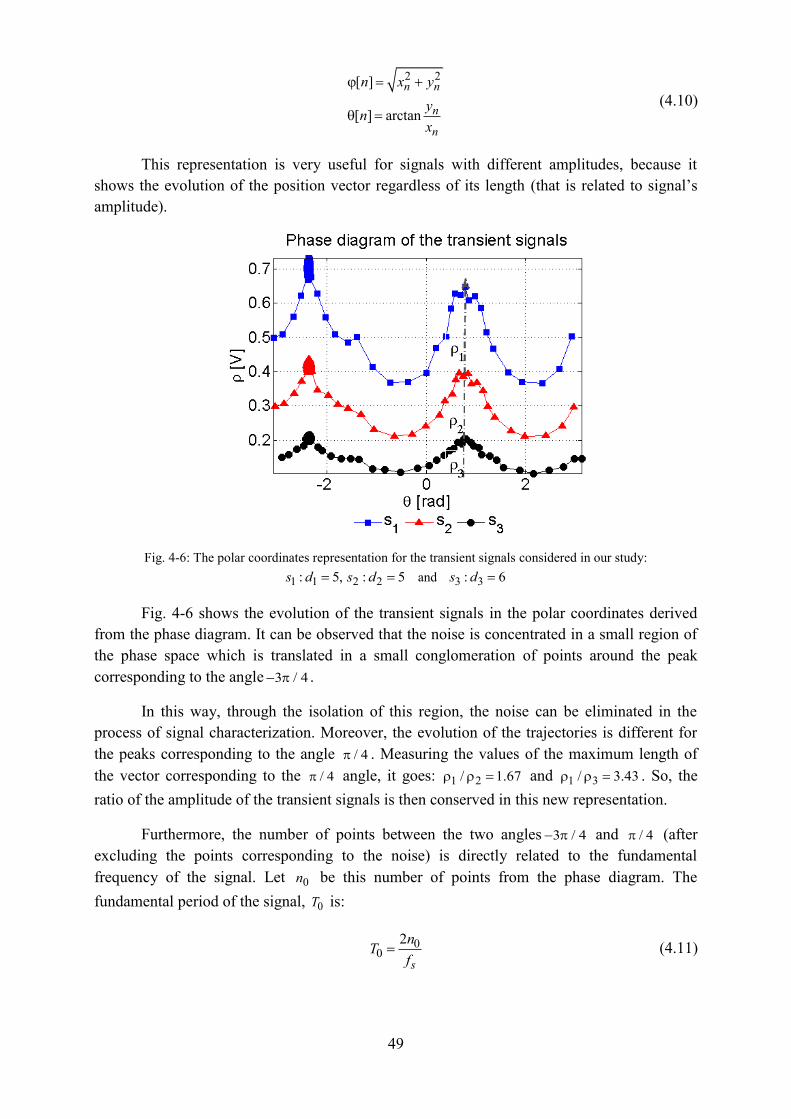
49
2 2[ ]
[ ] arctan
n n
n
n
n x y
yn
x
(4.10)
This representation is very useful for signals with different amplitudes, because it
shows the evolution of the position vector regardless of its length (that is related to signal’s
amplitude).
Fig. 4-6: The polar coordinates representation for the transient signals considered in our study:
1 1 2 2: 5, : 5s d s d and 3 3: 6s d
Fig. 4-6 shows the evolution of the transient signals in the polar coordinates derived
from the phase diagram. It can be observed that the noise is concentrated in a small region of
the phase space which is translated in a small conglomeration of points around the peak
corresponding to the angle 3 / 4 .
In this way, through the isolation of this region, the noise can be eliminated in the
process of signal characterization. Moreover, the evolution of the trajectories is different for
the peaks corresponding to the angle / 4 . Measuring the values of the maximum length of
the vector corresponding to the / 4 angle, it goes: 1 2/ 1.67 and 1 3/ 3.43 . So, the
ratio of the amplitude of the transient signals is then conserved in this new representation.
Furthermore, the number of points between the two angles 3 / 4 and / 4 (after
excluding the points corresponding to the noise) is directly related to the fundamental
frequency of the signal. Let 0n be this number of points from the phase diagram. The
fundamental period of the signal, 0T is:
00
2
s
nT
f (4.11)

50
From eq.(4.11), it goes that: 1 2/ 1.04f f and 1 3/ 1.24f f which are very close to the
ratios proposed in eq. (2.9). These results allow us to discriminate between the proposed
signals although their characteristics are very close.
Fig. 4-7: The schematic presentation of the multi-lag tools
Fig. 4-7 presents the MPLA algorithm divided in two parts: the elliptic modeling and
the polar coordinates representation, namely the phase diagram representation.
4.3. Diagonal lines quantification
The diagonal lines on the recurrence matrix indicate that the system returns in
approximately the same state for a certain period of time. The choice of the diagonal lines
quantification (DLQ - Diagonal Lines Quantification) is given by the fact that the distance
between two successive diagonal lines provides the fundamental period of the signal
(Digulescu, et al., 2016b), (Ioana, et al., 2014).
The quantification of these lines is done as follows:
,
1
1[ ] * , 0, 1
M n
i i n
i
dlq n D n MM n
(4.12)
where , , ,* 1 / max{ }i i n i i n i i nD D D is the complement of the distance matrix.
Then, the Fourier transform is applied to this quantification:
1
2 /
0
[ ] [ ]
Mj kn M
k
DLQ k dlq n e
(4.13)
where M is given in eq. (2.11). Fig. 4-8 presents the SD measure applied on a sine wave
with the frequency 10f Hz .

51
Fig. 4-8: Example of DLQ: (left) test signal – a sine wave with the frequency 10f Hz ; (center) the DLQ
measure; (right) zoom on the DLQ measure;
This approach points out the frequency component in a different manner than the
classical approach, where the Fourier transform is directly computed on the analyzed signal.
In this case, the choice of the distance matrix is preferable to the recurrence matrix in order to
follow the evolution of the signal entirely and not to separate it into a binary decision which
usually brings in the spectral content various harmonics.
To illustrate this concept, let us consider a signal composed by the product of two
cosines:
[ ] cos cos ,x n n n (4.14)
To simplify the demonstration, we suppose that the embedding dimension 2m and
the used distance is the squared Euclidean distance:
[ ] [ ]iv x i i x i d j (4.15)
Therefore the distance matrix depends on:
2 2,
2 2
[ ] [ ] [ ] ([ ]
[ ] [ ]
i i n
i i d
D x i x i n x i d x i n d
E n E n
(4.16)
Replacing eq. (4.14) in eq.(4.16), it goes that:
[2 ] [2 ]
[ ] 2 sin cos2 2
ii n i n
E n
(4.17)
where sin[( ) ] sin[( ) ]
2 2
n n considering the relationship between the frequencies
from eq. (4.14).
Using eq. (4.17)in eq. (4.16), leads to:
2 2[ ] 1 cos 2 cos 2 cos (2 ) cos[ (2 )]2 2
in n
E n i i i n i n
(4.18)
The eq. (4.18) develops the spectral representation of the diagonal lines quantification.
Together with the component that it is also found in the classical approach, in this
representation there are present two other components: a component at 2 and another at 2 .

52
To exemplify our approach, let [ ]x n be a test signal:
1 2[ ] cos[2 ] cos[2 ]x n f n f n (4.19)
where 1 500f Hz and 2 39f Hz , conserving the condition . The test signal is shown
in Fig. 4-9.
Fig. 4-9: The time evolution of the test signal modulated in amplitude
Fig. 4-10: The spectral representation of the diagonal lines quantification (up - left), the classical amplitude
spectrum representation (up – right) and the envelope amplitude spectrum (down – center); for the computation
of the distance matrix, it is used the squared Euclidean distance, 3m and 2d

53
Fig. 4-10 presents the new information brought by this new approach: the diagonal
lines representation contains three important components ( 2 , ,2 ), while the amplitude
spectrum of the proposed signal presents only the component and the envelope
amplitude spectrum contains only the envelope frequency information, but also multiple
harmonics of its envelope.
The displayed data tips show the values of the components: 78f Hz , two
components at 500 39f Hz and the third at 2(500 39)f Hz and 2 500f Hz . It is
obvious that the classical amplitude spectrum contains only the frequency 500 39f Hz and
the envelope amplitude spectrum the frequency 78 , {1,2,3,...}f k Hz k .
This new quantification is very useful for applications where wide band signals
interact with low frequencies which is the case of vortex detection and characterization: the
wide band signals are suitable hydraulic system monitoring (Candel, et al., 2014a),
(Digulescu, et al., 2014d), (Digulescu, et al., 2016a), (Digulescu, et al., 2016b) and the
frequencies induced by the vortex are significantly smaller than the wide band signals
(Digulescu, et al., 2016a).
It should be noticed that, when , the frequency modulation amplitude spectrum
is quite similar with the amplitude spectrum of the amplitude modulation. Therefore, we apply
the diagonal line quantification on the next test signal (Fig. 4-11):
1 2[ ] cos[2 cos[2 ]]x n f n f n (4.20)
where 1 500f Hz and 2 39f Hz and 2 . The condition stands valid.
Fig. 4-11: The frequency modulated test signal
From Fig. 4-12, it can be noticed that in the case of a frequency modulated signal, the
diagonal line quantification measure also emphasizes the classical components , but
more important the extra component . Besides an extra component 2( ) .

54
Fig. 4-12: The classical amplitude spectrum representation (left) and the spectral representation of the diagonal
lines quantification (right); for the computation of the distance matrix, it is used the squared Euclidean distance,
3m and 2d
This approach is very useful for applications where a phenomenon of interest is
characterized by much lower spectral content than the investigating signal’s one.
4.4. Chapter summary
This chapter presents new approaches for the detection, localization and
characterization of transient signals using the RPA, RQA and the phase diagram analysis
concept. The TDR measure is based in the evolution of the signal in phase space and it
exploits the recurrence matrix properties in order to detect and localize transient signals.
Next, the MLPA is introduced based on the elliptic modeling and on the phase
diagram representation. This type of analysis is very useful for the discrimination of signals
with close parameters.
Finally, the diagonal lines quantification is introduced and, using synthetic signals, we
emphasize the attributes that this type of quantification makes visible: the modulating
component of an amplitude/ frequency modulated signal, even if they are much lower in
frequency than the investigating signal’s content.
55
CHAPTER 5
5. Applications in active configurations
This chapter focuses on the experiments performed in active configuration. Firstly, we
present the experimental configuration and, then, we show our results using the theoretical
methods presented in the previous chapter. Moreover, these results are compared with
classical methods.
5.1. Cavitating environments
The first applicative context is the detection of the cavitating vortex based on non-
intrusive active sensing using an ultrasonic path defined by two wide band transducers. The
objective of this application is to emphasize the effect of the cavitating vortex from the
acoustic data in order to identify the different phases of the evolution of the phenomenon.
Measurements were carried out in a laboratory facility which materializes the flow conditions
downstream a hydraulic turbine.
The vortex flow and vortex spectrum
In literature the vortex vector is defined as 2u , where is the rotational
speed of the fluid (namely the local spinning motion in a given point) and u is the local flow
velocity vector. The flow for an incompressible fluid of velocity is described by the Navier-
Stokes (5.1) and continuity equations (5.2) (Emanuel, 1984), (Takahashi & Miyazaki, 2006):
21uu u=- up v
t
(5.1)
0u (5.2)
where p is the fluid pressure, is the density of the fluid, u is the flow velocity vector, v is
the fluid viscosity and is del operator.
For the vortex analysis, the Rankine model can be used. Analytically, the Rankine
vortex is defined by the components from eq. (5.3)(Takahashi & Miyazaki, 2006):
max max
max
maxmax max
,
0; 0;
,
r z
rv r r
ru u u
rv r r
r
(5.3)
where ,r zu u and u are the radial, axial and, respectively, tangential velocity components
defined in a cylindrical coordinate system for the u flow velocity. It should be mentioned

56
that, when maxr r , the tangential velocity u progresses in the forced vortex region, while,
when maxr r , its progress happens in the free vortex region.
The frequency signature of the cavitating vortex is given by the solution (5.3) of
equations (5.1) and (5.2) through the solution . Hereby, the relation between the vortex flow
and its spectrum is:
max
2max
max
,
0; 0;,
r z
r r r
u u u rr r
r
(5.4)
In (Rubin, 2000), there can be found more details about the spectral magnitude of
Doppler velocity. For our experiments, this theoretical result shows that the vortex conduct to
the generation of a low frequency component that our methodology aims to exploit in order to
assess this phenomenon.
5.1.1. Experimental configuration and results
The experiments have been conducted in a reduced scale facility which consisted of a
hydraulic installation where the flow rate can be manually changed (Candel, et al., 2014a).
The acoustic transceivers operate around at 1 MHz and the emitted waveform is a wide band
signal with the same central frequency. This signal, v( ) has a linear characteristic law.
20
( )( , ) cos( ( )), ( ) 2 2 ( ) ( )
d tv t t where t t f t t and t
dt
(5.5)
where 0 800 , [0,100 ]f kHz t s , the coefficient is chosen such that the final frequency of
the sweep is 1200f kHz .
Considering that the cavitating vortex is characterized by the unknown law ( )u and
the wide band signals (that are continuously emitted) are characterized by ( )v , then, at the
receiver, the signal carries the interaction between the emitted signal and the studied
cavitating vortex in ( , )w . The purpose of the experiment is to highlight the signature of the
cavitating vortex from the received signal.
The experiments are performed on two different pipelines; therefore, there are two
configurations to consider. The pipeline of the installation has been placed inside a stator
which produced the cavitational vortex as the flow rate increases, Fig. 5-1.
Fig. 5-1: The installation for the first set of measurements
There are two experimental setups that we performed: for the first one, the flow rate of
the hydraulic system varies and, when the flow rate becomes stable, the acoustic active

57
system is started at this operating point. In the same time, the flow rate of the system is
recorded. Moreover, on the tip of the stator a pressure sensor is placed so that we have a
reference for the cavitational vortex (more the pressure is dropping, higher the intensity of the
cavitation is). Fig. 5-2 presents the setup of the experiment.
Fig. 5-2: The on-site setup for the first set of measurements
The second experimental setup is performed after the divergent region of the Plexiglas
pipeline, as shown in Fig. 5-3 and Fig. 5-4.
Fig. 5-3: The installation for the second set of measurements
Fig. 5-4: The on-site setup for the second set of measurements
The experiment is done while slowly varying the flow rate of the water. In other
words, during the experiment, the received signal is acquired and recorded in bursts of 2.6 ms
simultaneously with the flow rate for approximately 90 s .
Fig. 5-5: Cavitating vortex stages: A1 no vortex (left), A2 incipient vortex (center), A3 developed vortex (right)
For both set of measurements, based on the visual observation (Fig. 5-5), three stages
of the vortex evolution were identified: A1 region - no vortex presence (up to 6 /l s ), A2
region incipient vortex (from 6 7.2 /to l s ) and A3 region developed vortex (more than
7.2 /l s ).

58
Relating the cavitating vortex stages to the deformation operator, we recall that:
when the water is monophasic: the deformation operator kD is defined by the attenuation
and delay:
( ) ( )k k ks t s t D (5.6)
where k is the index of the propagation path. Therefore, the received signal is:
( ) ( ) ( )k k
k
r t s t n t
when the cavitation appears: then, the deformation operator kD is characterized by
attenuation, delay, as well as the Doppler effect that acts as a deformation of the
instantaneous phase of the signal:
( ) ( ( )) exp( ( ))k k k k ks t s t t A j t D (5.7)
where ( )
( ) kk
r tt t
c
and ( )kr t is the time (Doppler) dependent position vector.
Based on this latter observation, we aim to detect and characterize this type of
environment.
First experimental setup
This experiment was performed in March, 2016 at the Power Engineering Faculty,
”Politehnica” University of Bucharest. The acoustic transducers are placed in “V”
configuration for a longer interaction with the vortex. The emission transducer, the closest to
the stator, generates 1 ms linear frequency modulations in a spectral bandwidth range of
[0.8,1.2] MHz with a repetition rate of 2.5 ms . The sampling frequency is 5MHz .
Fig. 5-6 presents the wide band acoustic signal used for the characterization of the
cavitational vortex and two received signals in different states of the system: for the incipient
cavitation, and for a fully developed cavitation, respectively.
Fig. 5-6: The emitted signal for each measurement, a received signal during a trial for the incipient cavitation
and a received signal during a trial for the cavitation flow

59
In Fig. 5-7 and Fig. 5-8, the limitations of the Fourier transform applied on the signal
and its envelope are presented. The signal considered is acquired when the cavitation is clear
eye visible (cavitation flow).
Fig. 5-7: The amplitude spectrum of the envelope for a received signal when the cavitational vortex is fully
developed
Fig. 5-8: The amplitude spectrum for a received signal when the cavitational vortex is fully developed
This approach is based on the assumption made in eq.(4.19), namely that the spectral
content of the cavitation has a much lower frequency content than the wide band acoustic
signal of the transceivers, . It can be seen that the associated phenomena (attenuation,
dispersion, noise, etc.) hide the effect induced by the particle motion from the cavitational
vortex, they only affect the low frequency content (around hundreds of Hz).
Fig. 5-9: The amplitude DLQ (eq. (4.13) ) for an acquired signal when the cavitational vortex is fully developed

60
On the other hand, the use of the diagonal line quantification (eq.(4.13)) highlights, on
the same signal, the cavitational vortex spectral content induced in the received signal when
the cavitation is fully developed (Fig. 5-9).
Next, we applied our approach for all acquired signals in each configuration. Table 5-1
presents the system’s characterizing parameters for each operating point of the system.
Operating
point no.
Parameters
Flow
rate
(l/s)
Mean
pressure
(bar)
Pressure
standard
deviation
(Pa)
3 1.14 1.23 1936
4 4.34 1.19 2437
5 9.2 1.05 3447
6 12.86 0.83 5784
7 14.77 0.64 6208
8 15.63 0.55 6985
9 16.01 0.51 7136
10 16.08 0.49 7039 Table 5-1: System’s parameters for each operating point
It should be noticed that the greater the number of the configuration is, the greater the
flow rate of the hydraulic system is. This has as a direct consequence the appearance of the
cavitation which is emphasized by the decreasing of the pressure and the increasing of its
standard deviation.
Fig. 5-10: The DLQ frequency position (left) and its mean (for 20 samples - right) using the diagonal lines
quantification approach for the signals acquired at each operating point (the number in red box indicates the
configuration); the RPA parameters are 5 3m and d using the Euclidean distance
As Fig. 5-10 presents, for the operating point no. 3, there is no cavitation. In operating
point no. 4, the mean of the frequency deviation increases as well as its standard deviation,
then, from operating point no. 5, the mean and the standard deviation of the frequency
component induced by the particle motion increase gradually. Moreover, the evolution of the
frequency component is strongly connected to the cavitating vortex stages shown in Fig. 5-5.
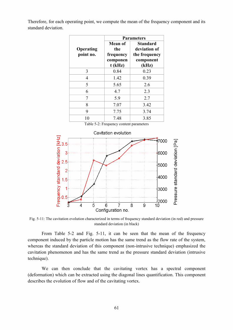
61
Therefore, for each operating point, we compute the mean of the frequency component and its
standard deviation.
Operating
point no.
Parameters
Mean of
the
frequency
componen
t (kHz)
Standard
deviation of
the frequency
component
(kHz)
3 0.84 0.23
4 1.42 0.39
5 5.65 2.6
6 4.7 2.3
7 5.9 2.7
8 7.07 3.42
9 7.75 3.74
10 7.48 3.85
Table 5-2: Frequency content parameters
Fig. 5-11: The cavitation evolution characterized in terms of frequency standard deviation (in red) and pressure
standard deviation (in black)
From Table 5-2 and Fig. 5-11, it can be seen that the mean of the frequency
component induced by the particle motion has the same trend as the flow rate of the system,
whereas the standard deviation of this component (non-intrusive technique) emphasized the
cavitation phenomenon and has the same trend as the pressure standard deviation (intrusive
technique).
We can then conclude that the cavitating vortex has a spectral component
(deformation) which can be extracted using the diagonal lines quantification. This component
describes the evolution of flow and of the cavitating vortex.

62
Second experimental setup
This experiment was performed in December, 2015 at the Power Engineering Faculty,
”Politehnica” University of Bucharest. In this setup, the stator is placed 70 mm upstream the
divergent section (previously, it was situated at 250 mm ). For the acoustic analysis, two pairs
of transceivers positioned in “V” configuration were used (Fig. 5-3 and Fig. 5-4) instead of
only one. Moreover, the transducers were placed further downstream from the cavitating
vortex area, on the divergent section (Fig. 5-3), while in the previous studies they were placed
on top of the cavitating vortex area.
The first set of data is obtained for the appearance and developing of the cavitating
vortex during discharge increasing. In order to cover the damping behavior of the cavitating
vortex from a hydraulic turbine, the variation of the discharge is reversed in the setup, so the
effect of the cavitating vortex disappearance was created.
We recall that the experiment is performed with a continuous slow variation of the
water flow. During the experiment, the water flow is varied from 6 19 /to l s and backwards,
in order to determine the critical flow rates for which the cavitating vortex appears/dampens.
Using the property of the diagonal line quantification, the position of the
component (attributed to the presence of cavitaing vortex) from the absolute value of SD
measure is determined for each burst of 2.6 ms in each vortex region. Further, an example of
component identification is presented in Fig. 5-12 and Fig. 5-13.
Fig. 5-12: DLQ absolute value for an acquisition of 2.6ms in A1 region
Fig. 5-13: DLQ absolute value for an acquisition of 2.6ms in A3 region
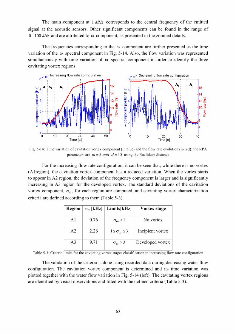
63
The main component at 1 MHz corresponds to the central frequency of the emitted
signal at the acoustic sensors. Other significant components can be found in the range of
0 100 kHz and are attributed to component, as presented in the zoomed details.
The frequencies corresponding to the component are further presented as the time
variation of the spectral component in Fig. 5-14. Also, the flow variation was represented
simultaneously with time variation of spectral component in order to identify the three
cavitating vortex regions.
Fig. 5-14: Time variation of cavitation vortex component (in blue) and the flow rate evolution (in red); the RPA
parameters are 5 15m and d using the Euclidean distance
For the increasing flow rate configuration, it can be seen that, while there is no vortex
(A1region), the cavitation vortex component has a reduced variation. When the vortex starts
to appear in A2 region, the deviation of the frequency component is larger and is significantly
increasing in A3 region for the developed vortex. The standard deviations of the cavitation
vortex component, , for each region are computed, and cavitating vortex characterization
criteria are defined according to them (Table 5-3).
Region [kHz] Limits[kHz] Vortex stage
A1 0.76 1 No vortex
A2 2.26 1 3 Incipient vortex
A3 9.71 3 Developed vortex
Table 5-3: Criteria limits for the cavitating vortex stages classification in increasing flow rate configuration
The validation of the criteria is done using recorded data during decreasing water flow
configuration. The cavitation vortex component is determined and its time variation was
plotted together with the water flow variation in Fig. 5-14 (left). The cavitating vortex regions
are identified by visual observations and fitted with the defined criteria (Table 5-3).
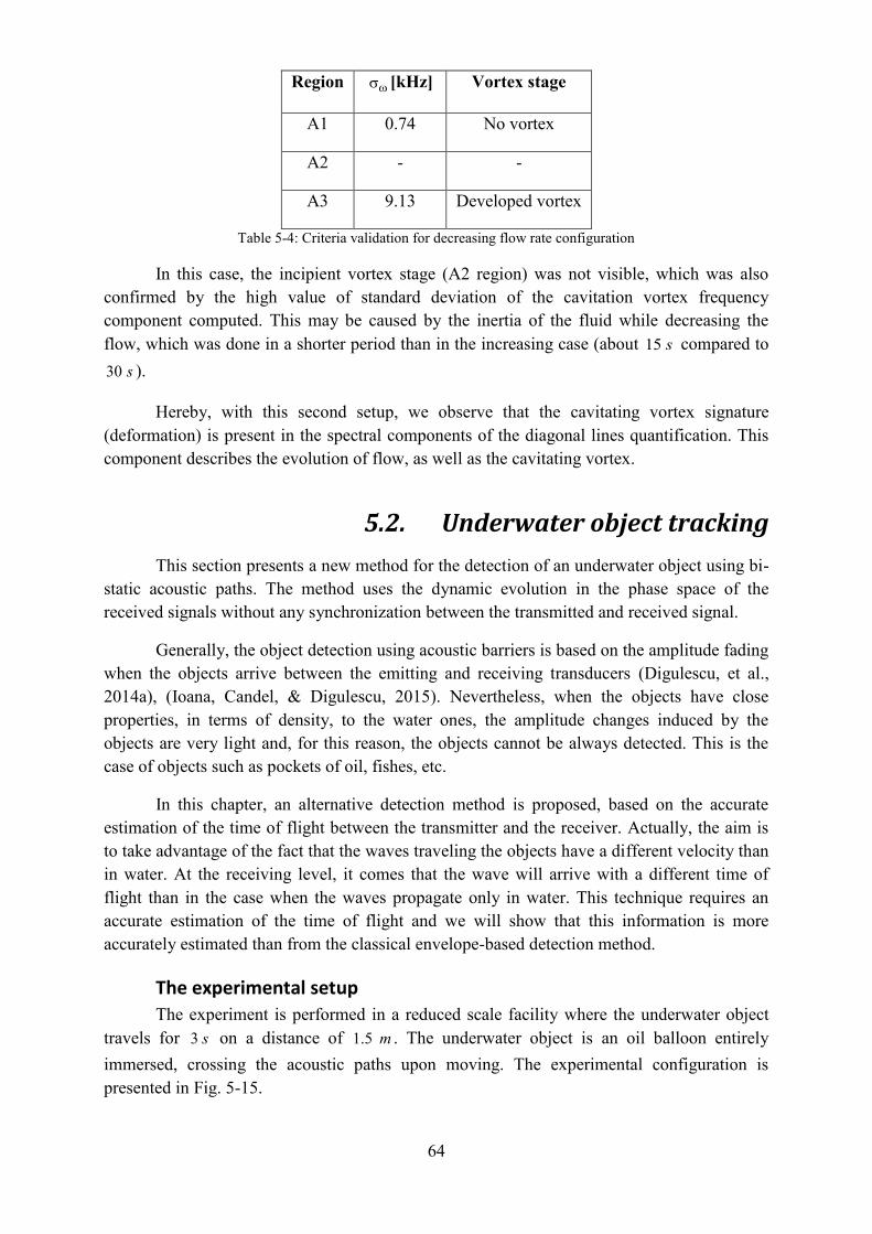
64
Region [kHz] Vortex stage
A1 0.74 No vortex
A2 - -
A3 9.13 Developed vortex
Table 5-4: Criteria validation for decreasing flow rate configuration
In this case, the incipient vortex stage (A2 region) was not visible, which was also
confirmed by the high value of standard deviation of the cavitation vortex frequency
component computed. This may be caused by the inertia of the fluid while decreasing the
flow, which was done in a shorter period than in the increasing case (about 15 s compared to
30 s ).
Hereby, with this second setup, we observe that the cavitating vortex signature
(deformation) is present in the spectral components of the diagonal lines quantification. This
component describes the evolution of flow, as well as the cavitating vortex.
5.2. Underwater object tracking
This section presents a new method for the detection of an underwater object using bi-
static acoustic paths. The method uses the dynamic evolution in the phase space of the
received signals without any synchronization between the transmitted and received signal.
Generally, the object detection using acoustic barriers is based on the amplitude fading
when the objects arrive between the emitting and receiving transducers (Digulescu, et al.,
2014a), (Ioana, Candel, & Digulescu, 2015). Nevertheless, when the objects have close
properties, in terms of density, to the water ones, the amplitude changes induced by the
objects are very light and, for this reason, the objects cannot be always detected. This is the
case of objects such as pockets of oil, fishes, etc.
In this chapter, an alternative detection method is proposed, based on the accurate
estimation of the time of flight between the transmitter and the receiver. Actually, the aim is
to take advantage of the fact that the waves traveling the objects have a different velocity than
in water. At the receiving level, it comes that the wave will arrive with a different time of
flight than in the case when the waves propagate only in water. This technique requires an
accurate estimation of the time of flight and we will show that this information is more
accurately estimated than from the classical envelope-based detection method.
The experimental setup
The experiment is performed in a reduced scale facility where the underwater object
travels for 3 s on a distance of 1.5 m . The underwater object is an oil balloon entirely
immersed, crossing the acoustic paths upon moving. The experimental configuration is
presented in Fig. 5-15.

65
Fig. 5-15: The experimental configuration: the dash-dot line shows the trajectory of the object
All four acoustic transducers are identical and have a wide band reception centered on
1 MHz with a bandwidth that starts from 800 kHz and ends around 1200 kHz . The amplitude
of the transmitted signal is 5 V. The emission transducers (Tx1 and Tx2) are placed on one
side of the water tank and generate linear chirp burst in their bandwidth at an angle of 45 . On
the opposite side of the water tank, the receiving sensors are placed at a minimum distance
such that crosstalk between the acoustic paths is avoided in the clear water (when no object is
in the water tank). The data acquisition is performed for duration of approximately 3.35 s in
order to record the entire process.
In this case, the deformation operator that we look to estimate is:
0( ) exp , 1,krkk k
water oil
drs t A j t k N
c c
D (5.8)
where kr is the thk water propagation path, kr
d is the thk oil propagation path and
02 b
rubber
l
c where bl is the thickness of the rubber wall of the balloon and rubberc is the
acoustic propagation velocity in rubber.
Results
Taking into account that the passage of the object in front of the sensors, involves a
change in the received time series, we aim to highlight this effect on the detection map based
on the *TDR measure (eq. (4.2)). Hereby, we define the detection map (Digulescu, et al.,
2015a):
*
1,
( , ) [ ( )]N
s
DM l TDR l
(5.9)
where N is the length of the recorded signal and s is the size of the fixed time bin for which
the *TDR measure is computed.
The detection map contains both the amplitude (in the *TDR measure) and time of
arrival information (given by the time bin, ). Therefore, this approach presents the time
information, although the signals have no synchronization and their characterization is based
only on the received signals by the two sensors.

66
For the detection part, we firstly present the signal recorded at Rx2 sensor (Fig. 5-15)
which directly receives its bursts from Tx2. On this signal, Fig. 5-16, the detection map based
on the *TDR measure is applied, Fig. 5-17.
Fig. 5-16: The recorded signal arrived at Rx2 sensor
Fig. 5-17: The detection map obtained for the Rx2 signal for 3m , 13d and 0.5
It can be observed that the burst (the response of the object) is represented by the two
brown horizontal lines which vary in amplitude (the average distance in the phase space
changes), but also in time (the TOAs of the bursts in each time bin is not constant). Moreover,
as the lines of the detection map represent the value of the *TDR measure at each time bin, its
columns contain the information regarding the TOAs of each burst at its corresponding time
bin.
Therefore, in order to obtain the TOA information from the detection map (Fig. 5-17),
we impose an appropriate threshold that discriminates between the part of the signal that has
no burst and the one that has it. In this case, the threshold is given by the cyan region from the
detection map. Hereby, the first point on each column of the detection map corresponding to
the cyan region gives the TOA of the responses in each time bin. The results are presented in
Fig. 5-18.

67
Fig. 5-18: The TOAs (red) of each response of Rx2 signal and its signal envelope (black)
Although, the signal’s envelope does not offer reliable information regarding the
object tracking (the amplitude variation can be caused by external vibrations, move of
transducers, etc.), the TOA information is very robust, because it highlights the delay induced
by the object. From Fig. 5-18, it can be seen that, even for a slight attenuation in signal’s
amplitude, the detection map approach is able to highlight a delay in the TOA of the burst for
two time bin intervals.
This delay is explained by the fact that the speed of sound in the sunflower oil is
smaller (around 1425 /m s ) than the water speed of sound (around 1480 /m s ) and its
maximum corresponds to the delay induced by the oil ball diameter (15 cm ) and the rubber
wall ( 0.5 mm ) of the balloon that folds the oil ball.
Moreover, in the TOA based object detection representation, the first interval
corresponds to the object passing in front of the transducer Tx2 and the second corresponds to
the crosstalk induced by the dispersion of the signals coming from Tx1. In this way, we
suppose that the travel direction of the object is from Tx2 to Tx1. In order, to confirm our
assumption, we also study the signals recorded by Rx1 (Fig. 5-19).
Fig. 5-19: The recorded signal arrived at Rx1 sensor
In this case, the signal is more disturbed in terms of amplitude. Fig. 5-20 and Fig. 5-21
present the detection map corresponding to the Rx1 signal and the TOAs of the responses
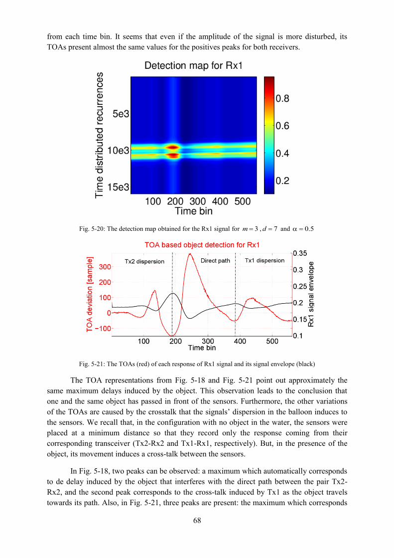
68
from each time bin. It seems that even if the amplitude of the signal is more disturbed, its
TOAs present almost the same values for the positives peaks for both receivers.
Fig. 5-20: The detection map obtained for the Rx1 signal for 3m , 7d and 0.5
Fig. 5-21: The TOAs (red) of each response of Rx1 signal and its signal envelope (black)
The TOA representations from Fig. 5-18 and Fig. 5-21 point out approximately the
same maximum delays induced by the object. This observation leads to the conclusion that
one and the same object has passed in front of the sensors. Furthermore, the other variations
of the TOAs are caused by the crosstalk that the signals’ dispersion in the balloon induces to
the sensors. We recall that, in the configuration with no object in the water, the sensors were
placed at a minimum distance so that they record only the response coming from their
corresponding transceiver (Tx2-Rx2 and Tx1-Rx1, respectively). But, in the presence of the
object, its movement induces a cross-talk between the sensors.
In Fig. 5-18, two peaks can be observed: a maximum which automatically corresponds
to de delay induced by the object that interferes with the direct path between the pair Tx2-
Rx2, and the second peak corresponds to the cross-talk induced by Tx1 as the object travels
towards its path. Also, in Fig. 5-21, three peaks are present: the maximum which corresponds
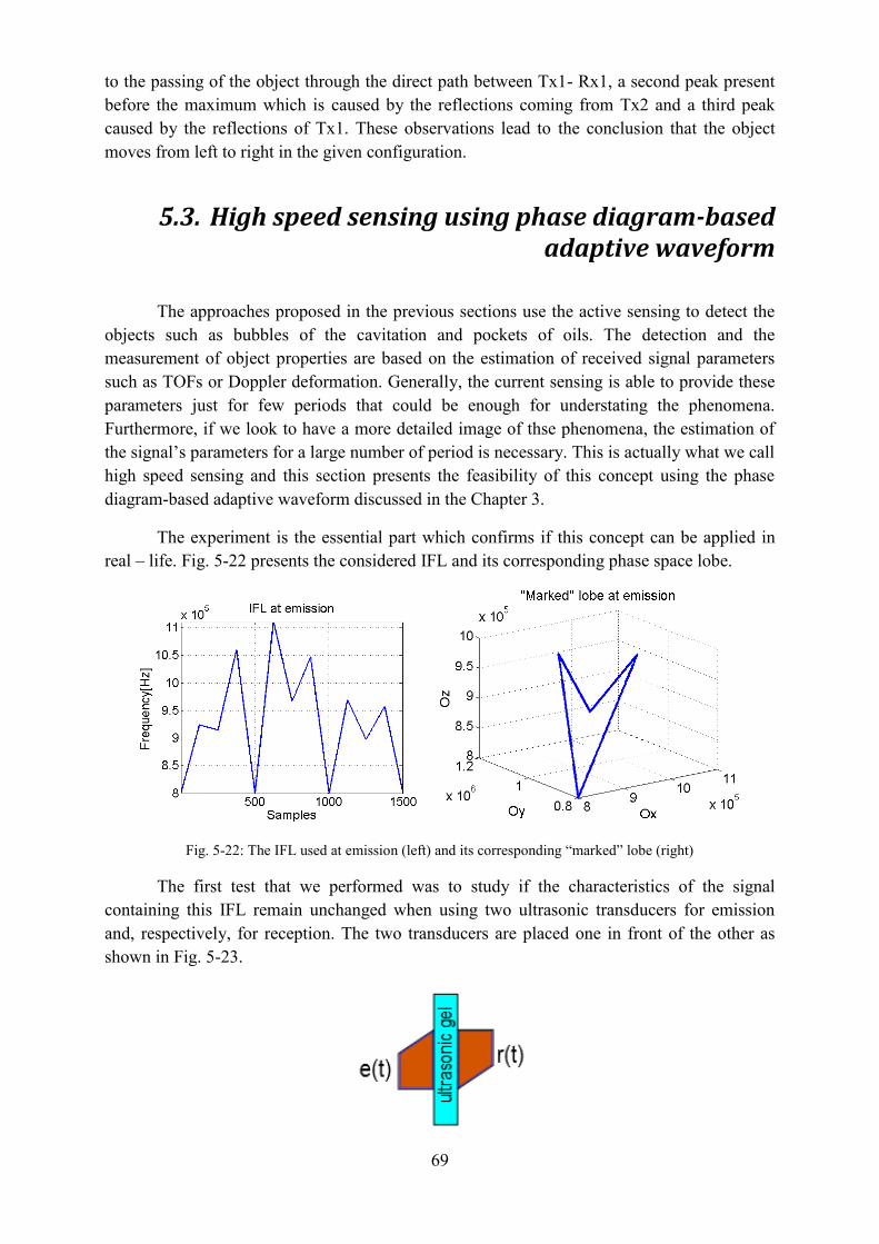
69
to the passing of the object through the direct path between Tx1- Rx1, a second peak present
before the maximum which is caused by the reflections coming from Tx2 and a third peak
caused by the reflections of Tx1. These observations lead to the conclusion that the object
moves from left to right in the given configuration.
5.3. High speed sensing using phase diagram-based adaptive waveform
The approaches proposed in the previous sections use the active sensing to detect the
objects such as bubbles of the cavitation and pockets of oils. The detection and the
measurement of object properties are based on the estimation of received signal parameters
such as TOFs or Doppler deformation. Generally, the current sensing is able to provide these
parameters just for few periods that could be enough for understating the phenomena.
Furthermore, if we look to have a more detailed image of thse phenomena, the estimation of
the signal’s parameters for a large number of period is necessary. This is actually what we call
high speed sensing and this section presents the feasibility of this concept using the phase
diagram-based adaptive waveform discussed in the Chapter 3.
The experiment is the essential part which confirms if this concept can be applied in
real – life. Fig. 5-22 presents the considered IFL and its corresponding phase space lobe.
Fig. 5-22: The IFL used at emission (left) and its corresponding “marked” lobe (right)
The first test that we performed was to study if the characteristics of the signal
containing this IFL remain unchanged when using two ultrasonic transducers for emission
and, respectively, for reception. The two transducers are placed one in front of the other as
shown in Fig. 5-23.

70
Fig. 5-23: The positioning of the two transducers for the experimental test
The signals used for emission and reception are shown in the next figure, Fig. 5-24.
Fig. 5-24: The signal used at emission and the received signal as well as their amplitude spectrum
Fig. 5-25: The IFLs of the emitted and received signals (left) and their representation in phase space (right)
From Fig. 5-25, it seems that, although the transfer characteristic of the transducers
eliminates part of the lower frequencies, the received signal maintains our proposed
characteristics. Therefore, these new signals with “special signatures” in the phase space can
be used in real-life applications.
The objective of the high-speed sensing using this waveform is to achieve a quasi-
continuous emission which contains overlapped signals in time, but separable using their
IFLs.
Hereby, considering the signal ( )s t , where:
1 2[ ] [ ] [ ]s n s n s n (5.10)
where 1[ ]s n and 2[ ]s n are the two signals with a unique representation in phase space and is
a delay which provides an initial time separation between the signals. Considering the phase
space representation of the phase space lobe, as shown in Fig. 5-26, is equal with 2N
where N is given in eq. (3.5).

71
Fig. 5-26: The time shifted IFLs used for overlapping where 1000N
Fig. 5-27: The overlapped signals which form the signal [ ]s n (left) and its spectrogram (right)
Fig. 5-28: Phase space lobes of the IFLs used for overlapping
Our objective is to separate the overlapped IFLs (Fig. 5-27) based on the algorithm
presented in Chapter 3. Considering the first IFL known (IFL1), we want to separate the
second IFL (IFL2) from the first, Fig. 5-28. Hereby, the algorithm is applied in the range
2 1 3N to N .

72
Fig. 5-29: The sum of the IFLs (left) and the phase space lobes of the IFL 2 (right)
Fig. 5-30: The sum of the IFLs (original – no noise, estimated – SNR=25 dB) (left) and the phase space lobes of
the IFL 2 (original – no noise, estimated – SNR=25 dB) (right)
This result, Fig. 5-29, shows that it is possible to separate two successive IFLs, which
correspond to our high speed sensing sequence, by looking on their trajectory in phase space.
Still, the method performs for quite high SNR (Fig. 5-30), the next research effort will attempt
to improve its noise robustness.
5.4. Chapter summary
In this chapter, we described our experiments performed in active configurations using
the theoretical methods introduced in this thesis.
For the cavitating environment application, we have shown that the generated vortex
flow can be characterized in a non-intrusive manner using the diagonal lines quantification for
of the received signal, when the phenomena are sensed with wide band signals.
The underwater object tracking is achieved using the *TDR measure detection map. We
point out the presence of the underwater object from the TOA parameter which is very robust
because it highlights the delay induced by the object, although the signal’s envelope is not
that reliable.

73
These two applications can be extended to a high speed sensing concept presented
after at the end of this Chapter, allowing to get the dynamic evolution of the cavitation
process or the object’s image, respectively. For this purpose, the phase diagram-based
waveform design can be successfully used, as illustrated in the final part of this chapter.

75
CHAPTER 6
6. Applications in passive configurations
This chapter presents the applications carried out in passive configuration. We present
the experimental configurations and, then, we show the results obtained using methods
proposed in the Chapter 4. Comparisons with classical method are performed.
6.1. Measuring pressure transient in water pipes
In this application, we present an acoustic signal processing approach for the
surveillance of a water pipe and the characterization of the water hammer effect. The
experiment is based on ultrasonic transceivers and the validation is made with intrusive
pressure sensors. The major objective is to quantify the pressure variation into the pipe using
a non-intrusive method that is usually used for the flow rate estimation (Wylie & Steerter,
1993). Therefore, the speed of the transient was determined using the time-of-flight (TOF)
estimated by the RQA method. The estimation of the pressure using the same electronic
device as for the flow rate estimation (Candel, et al., 2014), (Murgan, et al., 2016), (Petrut, et
al., 2014) would be a great achievement since it offers to an existing device a second
functionality.
In industrial applications, the water hammer must be supervised and controlled in
order to minimize the destructive effects that it may cause to the hydraulic system. For this
reason, the proposed approach that uses ultrasonic transceivers has the advantage to be
suitable for most systems since it does not require any extra manipulations upon the system or
pipeline.
6.1.1. Water hammer parameters
The water hammer is a periodic phenomenon caused by sudden maneuver of a closing
vane (fully or partial). This forced stopping of the flowing fluid particles implies changing of
their kinetic energy into pressure energy, so the pressure in the vane section will be increased
with p .
The maximum overpressure in a pipe during water hammer due to sudden total closure
of a vane can be determined using Joukowsky equation (Houghtalen, Akan, & Hwang, 2010),
(Hachem & Schleiss, 2012), (Wylie & Steerter, 1993):
0p c V (6.1)
where is the fluid density, c is the pressure wave velocity and 0V is the steady state flow
velocity.

76
Some part of the energy is dissipated due to fluid viscosity (so to the hydraulic losses)
which attenuates in time the water hammer phenomenon (Bucur, et al., 2014). The pressure
waves travel inside the pipe along its length, L , between the closing vane and the reservoir,
with high velocities, c , and have an oscillating period, T . Hereby, this period is given by:
4L
cT
(6.2)
Also, the pressure wave speed, c , can be determined considering the characteristics of
the fluid and of the pipe:
1
1
w
cD
e E
(6.3)
where w is the bulk modulus of the fluid, D is the pipe diameter, e is the pipe wall thickness
and E is the Young modulus of the pipe.
6.1.2. Experimental setup and results
The experimental setup (Fig. 6-1 and Fig. 6-2) consists in a horizontal pipe supplied
by a tank (ST) with a total volume of 200 l . Together with an air compressor, it can create
the constant supply pressures needed for the experiments.
The pipe has a length of 10.11L m , made entire of Plexiglas, with rectangular
exterior section of 250 50 mm and circular interior section, 39D mm , used for high quality
visualization of the process. The water is evacuated at the downstream end of the pipe through
an 20 mm orifice diaphragm ( d ).
Fig. 6-1: Experimental setup

77
Fig. 6-2: The on-site experimental setup of the ultrasonic transceivers performed at Power Engineering Faculty,
”Politehnica” University of Bucharest in December 2014
The discharge is regulated using a valve (RV) mounted at the entrance of the pipe, at
0.25 m downstream ST. The closing vane (CV) is a pneumatically driven butterfly with a
pneumatic actuator mounted together with the valve. The valve closing time is approximately
20 ms obtained with 4 bar of the air pressure in the valves actuators pneumatic circuit.
The pressure transducer P2 is mounted upstream the fast closing vane, at 2.05 m . It
has the measuring range between 0 40 bar relative pressure, with the output signal 0 10 V ,
accuracy 0.25 and repeatability 0.1% of full scale (Fig. 6-1 and Fig. 6-2).
Also, two acoustic transceivers were placed upstream the closing vane at 8 cm and
16 cm respectively (Fig. 6-1 and Fig. 6-2). The acoustic transceivers have a wide band
reception centered on 1MHz , but being able to receive signals starting from 8 kHz . The
output signal varies from 20 20V to V . Both transceivers were set in passive configuration
and the acquisition was made at a sampling frequency of 50 MHz for a period of 0.67 s .
The transient regime (water hammer) during the tests was induced by the sudden
closure of the vane CV. The initial conditions are 1.98 /l s flow rate and 1.4 bar supply
pressure. The maximum pressure due to water hammer phenomenon recorded by P2 during
tests was of 17.3 bar .
For this application, we recall that the deformation operator kD becomes:
( ) exp kk k
pressure
Ls t A j t
c
D (6.4)
where pressurec is the propagation speed of the pressure field and kL is the distance between
the CV and the ultrasonic transducers.

78
This deformation operator translates, at the transducers, transient signals which offer
the TOF information needed for the non-invasive pressure variation estimation.
Results using the RQA-based signal processing approach
The acquired acoustic signals at both sensors are presented in fig. 3. As the dashed
blue ellipse highlights, it can be observed that the acoustic transient happen simultaneously
with the pressure spikes. Moreover, as S2 is closer to the CV (approx. 8 cm ), the received
acoustic transients are much more visible (fig. 3(a)) than those arrived at S1 (fig. 3(b)). This is
because the water hammer acoustic wave starts to diffuse. Still, the acoustic transient at S1
has high energy (Digulescu, et al., 2015c).
Fig. 6-3: The acoustic signals recorded by the two sensor and the simultaneous pressure time evolution: (left)
acoustic signal arrived at sensor S2; (right) acoustic signal arrived at sensor S1
We applied the RPA method on these signals and computed the *TDR measure for
3, 10 70m d and .
Fig. 6-4: The water hammer effect detection on the signals recorded by the two sensors
In Fig. 6-4, it can be seen that the *TDR measure succeeds to detect the acoustic
transients regardless of mechanical vibrations and environmental noise recorded by the
sensors. In the computation of the TOF, we considered the first moments for which the *TDR
measure was 80% from the maxima, namely * 0.8TDR

79
Hereby, we determined that 82TOF s . Knowing that the distance between the two
ultrasonic sensors was 8sd cm , we obtained the wave speed 975 /TDRc m s .
Alternatively, considering just the maxima given by the acoustic transients (result
obtained typically from the envelope detection), we obtained 99TOF s , namely
805 /pkc m s . The difference between this approach and the RQA-based method is given by
the diffusion effect of the acoustic wave generated by the water hammer.
Results using Joukowski equation
In the given configuration, the theoretical value of pressure wave speed in a Plexiglas
pipe was computed using eq. (6.3) and considering the parameters of the water and the pipe as
given by Table 6-1.
Parameter Value
31000 /kg m
w 2.1 GPa
e 10 mm
E 5.66 GPa
Table 6-1: Characteristic parameters of the pipe and fluid for theoretical computation of the pressure wave
Also, the presence of four butterfly valves with steel casing situated along the pipe
was taken into account and an weighted elasticity modulus ( E ) of the setup was determined.
Hereby, the theoretical pressure wave speed value obtained is 926 /thc m s , value that
is closest to the one determined by the RQA-based method. Using this value, the pressure
variation during water hammer can be determined from eq. (6.1), and results a maximum
increase of 15.35thp bar .
Pressure variation
Using the maximum pressure difference measured during the tests after the sudden
closure of the vane, 15.9p bar , the experimental value of pressure wave speed can be
calculated with Joukowsky equation (6.1). In order to obtain this, the water velocity in the
steady state flow is determined from the continuity equation, 20 4 / ( )V Q D , as the flow rate
before the closure is 1.98 /Q l s . So, for the obtained value of 0 1.66 /V m s the resulted
experimental pressure wave speed is 959 /ec m s .
The results from Table 6-2 show that RQA approach gives very good results with an
estimation error below 2% . This may be caused by the choice of the threshold of the *TDR
measure. Further investigations will be made for improvement. The next suitable approach is
the one given by Joukowsky equation. Still, in industrial hydraulic systems, it may be difficult
to determine a correct elasticity modulus of the materials that may be degraded and changed
since their design, which will directly influence a correct evaluation of the pressure wave
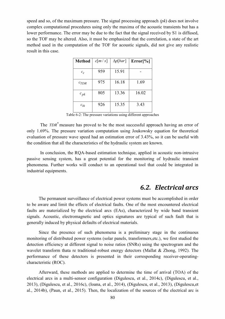
80
speed and so, of the maximum pressure. The signal processing approach (pk) does not involve
complex computational procedures using only the maxima of the acoustic transients but has a
lower performance. The error may be due to the fact that the signal received by S1 is diffused,
so the TOF may be altered. Also, it must be emphasized that the correlation, a state of the art
method used in the computation of the TOF for acoustic signals, did not give any realistic
result in this case.
Method [ / ]c m s [ ]p bar Error[%]
ec 959 15.91 -
TDRc 975 16.18 1.69
pkc 805 13.36 16.02
thc 926 15.35 3.43
Table 6-2: The pressure variations using different approaches
The *TDR measure has proved to be the most successful approach having an error of
only 1.69%. The pressure variation computation using Joukowsky equation for theoretical
evaluation of pressure wave speed had an estimation error of 3.43%, so it can be useful with
the condition that all the characteristics of the hydraulic system are known.
In conclusion, the RQA-based estimation technique, applied in acoustic non-intrusive
passive sensing system, has a great potential for the monitoring of hydraulic transient
phenomena. Further works will conduct to an operational tool that could be integrated in
industrial equipments.
6.2. Electrical arcs
The permanent surveillance of electrical power systems must be accomplished in order
to be aware and limit the effects of electrical faults. One of the most encountered electrical
faults are materialized by the electrical arcs (EAs), characterized by wide band transient
signals. Acoustic, electromagnetic and optics signatures are typical of such fault that is
generally induced by physical defaults of electrical materials.
Since the presence of such phenomena is a preliminary stage in the continuous
monitoring of distributed power systems (solar panels, transformers,etc.), we first studied the
detection efficiency at different signal to noise ratios (SNRs) using the spectrogram and the
wavelet transform thata re traditional-robust energy detectors (Mallat & Zhong, 1992). The
performance of these detectors is presented in their corresponding receiver-operating-
characteristic (ROC).
Afterward, these methods are applied to determine the time of arrival (TOA) of the
electrical arcs in a multi-sensor configuration (Digulescu, et al., 2014c), (Digulescu, et al.,
2013), (Digulescu, et al., 2016c), (Ioana, et al., 2014), (Digulescu, et al., 2013), (Digulescu,et
al., 2014b), (Paun, et al., 2015). Then, the localization of the sources of the electrical arc is

81
obtained by solving the geometrical system which describes the experimental configuration.
Finally, we presented the precision accuracy of each method.
Finally, we characterize these signals using the MLPA method in order to monitor the
signal’s changes, aiming to classify the electrical arc’s signature (Digulescu, et al., 2015b),
(Serbanescu, et al., 2015).
6.2.1. Detection performance
The experiment is performed with an electrical arc locator system composed of three
acoustical sensors placed in a 3D configuration and a wide band antenna placed in the center
of the system. The experimental configuration is presented in Fig. 6-5.
Fig. 6-5: The experimental configuration of the EA locator system
Fig. 6-6: The recorded EAs and the detection curve obtained with the TDR measure: 3, 8 0.7m d and
x y
z
S2S3S4
Electrical Arc
Photovoltaic panel
Wide band antenna

82
The detection and estimation of times of arrival of the transient signals generated by
electrical arc at each sensor has been done using the *TDR measure, the spectrogram and the
wavelet transform. Fig. 6-6 presents an example of received signals and their detection curves
obtained with the *TDR measure.
For the ROCs computation, we considered the following algorithm for the SNR value:
Let us consider that s is the test signal of length L
For a given SNR , we have: 10lg s n
n
P PSNR
P
, where
2
1
[ ]L
s
i
s iP
L
Hereby, we obtain
1010 1
sn SNR
PP
Then, the imposed noise is: 0 ,nn P n where 0n is a random signal with normal
distribution of mean zero and variance equal to 1
The studied signal becomes: ns s n
We compare the *TDR measure with the spectrogram and wavelet methods by
tracking the ROCs. The results are presented in Fig. 6-7.
Fig. 6-7: The detection performances of each method; the ROCs where computed for the same white additive
Gaussian noise (100 realizations) for each SNR level and method: (up-left) *TDR measure for
3, 8 0.7m d and ; (up-right) the spectrogram-based detection; (down) the wavelet-based detection
using the Mexican Hat mother function

83
As expected, both dedicated detection methods have the best performances which are
one size higher. Nevertheless, the RQA-based method, namely the *TDR measure offers
reliable performances, therefore, in the case of localization application, this approach must be
considered in terms of localization accuracy.
The signals (Fig. 6-6) are recorded at a sampling frequency of 5sf MHz for a period
of 10 ms ( 50000 samples). In terms of location accuracy, the *TDR measure is compared with
the classical time-scale approaches.
The spatial localization is achieved by solving the geometrical system (eq.(6.5)) based
on the time-of-arrival (TOA) of the EAs at each microphone. The TOA is obtained by
imposing the same threshold ( 0.5 ) at the normalized detection curves based on each method.
2 1
3 1
4 1
21
31
41
PS PS
PS PS
PS PS
d d v t
d d v t
d d v t
(6.5)
where 2 2 2( ) ( ) ( ) , 1,4i i i iPS s P s P s Pd x x y y z z i , each position of the acoustic
sensor and antenna (considered 1S ) is known ( , , )i i ii S S SS x y z , ( 1)i it is the time of arrival of
the EA at each microphone triggered by the 1S wide band antenna. The localization accuracy
using each method is presented in Table 6-3.
Method Relative error [%]
*TDR measure 6.2
Wavelet 11.2
Spectrogram 9.4
Table 6-3: The spatial localization accuracy for the electrical arcs
In this application, the signal is propagated on multiple paths, because the experiment
is performed in a closed facility: an indoor facility, mainly characterized by three propagation
paths.
Although, the classical techniques detect and localize the electrical arc source in an
effective manner, when it comes to multi-path signal discrimination, these methods are
limited.
But, the MLPA method provides better results. Using one of the signals arrived at 2S
microphone, the reflections 2 3,s s of the electrical arc are compared with the direct path signal
1s . These signals are presented in Fig. 6-8.

84
Fig. 6-8: The electrical arc recording 1s and its reflections 2 3,s s
For the multi-path acoustic signals, the elliptic modeling (eq.(4.9)) is applied and the
area of the estimated ellipse is determined (Fig. 6-9).
Fig. 6-9: The areas of the estimated ellipses that circumscribe the phase-space trajectory of the normalized multi-
path signals
The estimated ellipses evolve in a different manner, but they have the same trend.
After an average value of the area is chosen, 1A , an optimal lag is determined: 1 11d ,
2 12d and 3 8d . The results of the phase diagram representation are shown in Fig. 6-10.

85
Fig. 6-10: The polar coordinates representation for the multi-path acoustic signals: 1 11d , 2 12d and
3 8d
In terms of attenuation, the phase diagram points out the same information as the time
evolution of the signals. Moreover, the reflections present fewer curves with peaks than the
direct path of the signal. This means that the reflections contain fewer oscillations than the
direct signal, hereby, the reflections are dispersed.
Using eq.(4.11), it goes that: 1 2
/ 0.94s sf f and 1 3
/ 0.92s sf f , meaning that the
reflections suffer a time dilatation. Because the frequency ratios are close to 1 , it leads to the
idea that the signals have the same source, but on their propagation path, the reflections are
affected by multiple phenomena: diffusion, dispersion, attenuation, etc.
6.3. Chapter summary
This chapter presents two applications of passive sensing. For the pressure transient
measurement, we have shown that the RQA-based method for transient detection and time
localization is a method worth being considered for the phenomenon characterization.
Regarding the EA application, the RQA approach provides a better localization
accuracy than the time-scale methods (but similar detection performances) and with the use of
multi-lag phase-space analysis, it highlights new information regarding the characterization of
transient signals and the changes that they suffer in a realistic multi-path propagation
environment.

87
CHAPTER 7
7. Conclusions and perspectives
7.1. Work summary
The main objective of this work was to contribute to the analysis of signals related to
different physical phenomena, aiming to better understand them as well as to estimate their
parameters that are interesting from application point of view. Different applicative contexts
have been investigated in active and passive sensing configurations. For the active part, we
mention the monitoring of cavitation phenomena and its characterization for hydraulic system
surveillance. The second application of the active sensing is the underwater object detection
and tracking without synchronization between sensors. For the passive configuration, we
focus on the pressure transient analysis in water pipes investigation with a non-intrusive
method and on the surveillance of electrical power systems in the presence of transient
phenomena such as electrical arcs.
Despite the differences between the physical considerations, we propose a unique
mathematical model of the signals issued from the active/passive sensing system used to
analyze the considered phenomena.
Chapter 2 presents a state of the art of the techniques used for acoustic sensing
methods, from signal processing perspective, in dynamic configurations. Starting with the
well known analysis techniques based on energy methods and projective approaches (such as
wavelet transform), we focus our research to the data-driven analysis technique based on the
phase diagram concept.
Chapter 3 describes a new concept of active sensing system for analyzing dynamic
transient phenomena. For the emission part we propose the phase-space-based waveform
design that presents a unique shape in the phase space and which can be easily translated into
a signal. Starting from this unique shape, called phase space lobe, we translate the
representation into a time series (auxiliary signal). This time series carries the IFL
(Instantaneous Frequency Law) of the further emission signal. The main advantage of this
new concept is the capability to generate several transmitting signals, non-orthogonal in
time/frequency domain but orthogonal in the phase diagram representation space. For the
reception part, the IFL information is estimated in a phase space-based representation space.
This waveform design technique presents the interest to conduct to a high speed sensing
methods, very useful to monitor dynamic phenomena. This work will conduct to a patent
software that will be pended before the end of this year.
Chapter 4 focuses on the signal analysis based on the major information that can be
extracted from phase diagrams: the recurrence quantification analysis (RQA) based on the
recurrence plot analysis (RPA). We propose new tools for the investigation of the signals
characteristics. The first one is the TDR* measure (Time Distributed Recurrences) that

88
quantifies the recurrence/ distance matrix and it is used for the detection of transient signals.
The second one is the multi-lag phase analysis using multiple lags and it is successfully used
to discriminate between signals with close parameters. Finally, the diagonal lines
quantification of RPA matrix is proposed as an alternative for the analysis of modulated
signals.
Chapter 5 and 6 present the experimental results using the proposed theoretical
methods introduced by this thesis. The results are compared with classical techniques. The
cavitating environment (a major problem in hydraulic turbines) evolution on a small scale
facility is characterized using the diagonal lines quantification of the distance matrix
(Digulescu, et al., 2016) (Digulescu, et al., 2016) (Digulescu, et al., 2014).
A new method for the detection of an underwater object using bi-static acoustic paths
is presented. For this application of object tracking, the main advantage of the RQA and RPA
methods is that it uses only the signals arrived at reception (so there is synchronization-free
technique). Using the TDR* measure, we define the detection map based on this measure
which is more robust to noise than the signal’s envelope-based detection. This map contains
both amplitude and time information (Digulescu, et al., 2015a).
The water hammer phenomenon is pointed out through our non-intrusive approach
that proves to be the closest to the reference method. The effect of the phenomenon is
quantified using the TDR measure which is more robust to the effect of pressure wave
diffusion that takes place inside the pipe during the experiment (Digulescu, et al., 2015c).
The electrical arc application points out that our approach presents another detection
method based only on the RQA and RPA methods using the TDR measure (Bernard, et al.,
2016), (Candel, et al., 2012a), (Digulescu, et al., 2013), (Digulescu, et al., 2016c), (Digulescu,
et al., 2014b), (Digulescu, et al., 2014c). The localization accuracy outperforms the classical
non-stationary signals processing methods. Moreover, the signals are characterized and
discriminated using the concept of multi-lag phase space analysis (Bernard, et al., 2016)
(Digulescu, et al., 2015b) (Digulescu, et al., 2016c).
These applications can be extended to a high speed sensing concept, allowing to get
the dynamic evolution of the cavitation process or the object’s image, respectively. For this
purpose, the phase diagram-based waveform design can be successfully used, as illustrated in
this work.
7.2. Perspectives
This thesis is structured in two main parts, one theoretical and another one applicative,
where the theoretical contributions have been investigated in some applications of current
interest. Consequently, the perspectives of my work will be concentrated on two main
directions – theoretical and applicative. Since the both aspects are intimately related, I prefer
to present them in a merged manner.
The first theoretical works will concern the phase diagram-based adaptive waveform,
by investigating different partition of information in the phase diagram domain. The

89
organization of the information in lobes could be generalized in n-dimensional phase diagram
domain, creating also the possibility to design better separable waveform carrying, in the
same time, more information, bringing the modulations more robust and with better
performances in terms of parameters of estimation.
At the receiver level, we will investigate the capability of instantaneous frequency law
tracking in the phase diagram, trying to take advantage of the phase continuity of the phase
trajectory. Namely, the IFL tracking can be successfully based on the association of the time-
frequency points according to the continuity criteria that could be naturally defined in the
phase diagram domain. In the case of the multi-lag phase diagram analysis, this continuity
will be defined in more robust manner since the random noise effect will be minimized when
looking to different lags.
In the applicative context, these new theoretical directions will conduct to the
definition of a new imaging acoustic methodology where the high speed sensing will be
allowed thanks to the construction of agile wide band waveforms, emitted as much lower PRF
than the classical ones. In addition, the accurate estimation of the received signals
characteristics will allow to form the acoustic images not only from the times of arrival, but
also from the relative deformation between the received signals.
Another applicative extension of this new theoretical work will concern the definition
of new communication modulations and multiple access technique, not only in acoustic but
also electromagnetic waves.
The second theoretical direction is the development of new signal descriptors in the
phase diagram plan. As a potential idea we mention here the dynamic of position vector in
polar coordinates, but merged from coherent variations of this vector at different lags.
Another work idea is to generalize the definition of these vectors in n-D. The
definition of a two-dimensional representation of the position vector parameters (calculated in
n-dimensional phase diagram coordinates) – representation similar to RPA, would be very
helpful for the intuitive data interpretation.
The relation between phase diagram analysis and the compressive sensing domain
could be also another work direction worth to be followed.
In the applicative context, the aforementioned directions will conduct to new methods
for signal analysis and characterization. Their using in the application we have investigated in
this thesis is natural. Namely, these representation methods will conduct to a finer analysis of
the interaction between acoustic waves and the hydrodynamic phenomena. The further
contribution will be to help in monitoring hydraulic machines in non-stationary conditions
that are nowadays under intensive multidisciplinary research works.
Another applicative work context of the further representation tools is the analysis of
the electromagnetic transients, aiming to characterize and localize their sources. Applications
in ultra wideband tracking, identification and communications as well as in monitoring of
power equipments are just two domains where the further theoretical researches will serve.


91
Résume étendu
Caractérisation des phénomènes dynamiques
à l’aide de l’analyse du signal
sur le diagramme des phases
La déformation des signaux au long de leur trajet de propagation est un des plus
importants facteurs qui doivent être considérés à la réception. Ces effets sont dus à des
phénomènes comme l’atténuation, la réflexion, la dispersion ou, encore, le bruit. Alors que les
premiers deux phénomènes sont assez facile à surveiller, parce qu’elles affectent l’amplitude,
respectivement le retard des signaux, les deux derniers phénomènes sont plus difficiles à
contrôler, parce qu’elles changent les paramètres du signal (amplitude, fréquence et phase) de
manière totalement dépendante de l’environnement.
Nous définissons un modèle générale pour le signal reçu après la propagation dans un
environnement hétérogène :
( ) ( ) ( )k
k
r t s t n t D (6)
où k D est l’operateur général de déformation associé à la composante k du signal reçu et
( )n t est le bruit additive blanc gaussien.
Dans cette thèse, l’objectif principal est de contribuer à l’analyse des signaux liés aux
différents phénomènes physiques, en visant une meilleure compréhension de ces phénomènes,
ainsi que l’estimation de leurs paramètres qui sont intéressants de point de vue applicatif.
Plusieurs contextes applicatifs ont été investigués dans deux configurations de mesure: active
et passive.
Pour la configuration active, le premier contexte applicatif consiste en l’étude du
phénomène de cavitation dans le domaine de la surveillance de systèmes hydrauliques. La
deuxième application de la configuration active est la détection et le suivi des objets
immergés sans synchronisation entre les capteurs d’émission et de réception.
Pour la configuration passive, nous nous concentrons sur l’analyse des transitoires de
pression dans les conduites d’eau en utilisant une méthode non-intrusive ainsi que sur la
surveillance des réseaux d’énergie électrique en présence des phénomènes transitoires comme
les arcs électriques.

92
Malgré les différences entre les considérations physiques spécifiques à ces
applications, nous proposons un modèle mathématique unique pour les signaux issus des deux
types de configuration.
Le Chapitre 2 présente les techniques les plus utilisés pour les méthodes de mesure
acoustique en configurations dynamiques, dans la perspective du traitement du signal. En
commençant avec les techniques d’analyse très connues basées sur l’approche énergétique
ainsi que sur les approches projectives (comme la transformée en odelettes), nous concentrons
notre recherche sur les techniques d’analyse des signaux aiguillées par les données.
La méthode des récurrences commence en considérant la série de temps suivante :
[1], [2],..., [ ]x x x x N (7)
Cette série est ensuite représentée dans l’espace des phases. Ses valeurs deviennent les
coordonnées de l’espace m - dimensionnel et, par conséquence, les vecteurs de l’espace est :
1
[ ( 1) ] , 1,m
i k
k
v x i k d e i M
(8)
où m est la dimension de l’espace, d est le retard entre les échantillons, ke est le vecteur
unitaire des axes de l’espace, ( 1)M N m d et N est la longueur de la série de temps.
Usuellement, la dimension de l’espace et le retard sont choisis en utilisant la méthode de faux
voisins et, respectivement, la méthode de l’information mutuelle.
Par la suite, les distances entre les vecteurs de l’espace des phases sont représentées
par la matrice des distances (DM), eq. (4). Comparées avec un seuil, on obtient la matrice des
récurrences (RM), eq. (2.13).
, ( , )i j i jD v vD (9)
, ( ) ( , )i j i jR i v v D (10)
où ( , ) D est la distance appliquée aux vecteurs de l’espace des phases (la distance
euclidienne, la norme L1, la distance angulaire), ( ) est la fonction Heaviside et ( )i est le
seuil considéré pour la récurrence.
L’avantage majeur de la méthode des récurrences est qu’elle ne requit aucune base
orthogonale ou aucune information apriori du système étudié (contrairement à la méthode des
ondelettes qui nécessite la définition d’un dictionnaire qui doit ressembler aux composantes
du signal analysé). La méthode fonctionne pour des applications où la référence n’est pas
disponible (contrairement à la méthode du filtrage adapté) et est plus précise pour la
localisation.
Le Chapitre 3 décrit un nouveau concept d’un système actif pour l’analyse des
phénomènes transitoires dynamiques. Pour la partie d’émission, nous proposons la
construction des ondes d’émissions basées sur l’espace des phases. Les différentes ondes
construites présentent une forme unique dans l’espace des phases.

93
Fig. 1:Le lobe dans l’espace des phases et son signal auxiliaire correspondant
En commençant avec cette forme unique, appelée lobe dans l’espace des phases, nous
translatons cette représentation dans une série temporelle (signal auxiliaire) (Fig. 1). Cette
série temporelle porte la LFI (Loi de Fréquence Instantanée) du signal d’émission. L’avantage
principal de ce concept est la capacité de générer plusieurs signaux à l’émission, non-
orthogonaux dans le domaine de temps et de fréquence, mais qui est orthogonal dans l’espace
de représentation constitué par le diagramme de phases.
Pour la partie de réception, l’information portée par la LFI est estimée dans une
analyse des trajectoires dans l’espace des phases (Fig. 2).
Fig. 2: Les LFI et leurs lobes multiples obtenus dans l’espace des phases
Cette technique de construction des formes d’ondes présente l’intérêt de conduire à
des méthodes d’investigation actives à haute cadence, très utiles pour la surveillance des
phénomènes dynamiques.
Le Chapitre 4 concerne l’analyse des signaux basée sur l’information majeure qui peut
être extraite du diagramme des phases : l’analyse des récurrences. Nous proposons deux
approches nouvelles pour l’investigation des caractéristiques des signaux. La première est la
mesure TDR* (Time Distributed Recurrences) qui quantifie la matrice des récurrences/
distances et qui est utilisée pour la détection des signaux transitoires.
La deuxième approche est l’analyse des phases à plusieurs retards et elle est utilisée
pour la discrimination entre des signaux avec des paramètres très proches. Finalement, la
quantification des lignes diagonales de la matrice des récurrences est proposée comme
alternative pour l’analyse des signaux modulés en fréquence.

94
Les Chapitres 5 et 6 présentent les résultats expérimentaux en utilisant les méthodes
théorétiques proposées dans cette thèse. Les résultats sont comparés avec des techniques
classiques. L’évolution de l’environnement avec de la cavitation (un problème majeure dans
la surveillance des installations hydrauliques) est caractérisée avec la quantification des lignes
diagonales de la matrices des distances (Fig. 3).
Fig. 3: La caractérisation du vortex avec des cavitations (générées par l’écoulement à l’interface avec un stator)
en utilisant la quantification des lignes diagonales de la matrice des distances
Fig. 4: La carte de détection basée sur la mesure TDR* et la détection de l’objet immergé en utilisant le temps
d’arrivé de chaque pulse
Une méthode nouvelle pour la détection d’un objet immergé en utilisant deux trajets
acoustiques statiques est également présentée. Pour l’application de suivi d’objet, l‘avantage
principal de la méthode des récurrences est qu’elle utilise seulement les signaux arrivés à la
réception (par ailleurs, elle est une technique qui ne nécessite pas la synchronisation). En
utilisant la mesure TDR*, nous définissons une carte de détection basée sur cette mesure qui

95
est plus robuste au bruit que la détection basée sur l’enveloppe du signal (Fig. 4). Cette carte
contient les deux informations de temps et d’amplitude.
Le phénomène de coup de bélier est également un autre contexte applicatif étudié par
notre approche non-intrusive qui montre qu’elle est la plus proche de la référence. L’effet du
phénomène est quantifié en utilisant la mesure TDR* (Fig. 5) qui est plus robuste à l’effet de
diffusion de l’onde de pression qui se passe à l’intérieur de la conduite pendant l’expérience
(erreur d’estimation sous 2%).
Fig. 5: La caractérisation du coup de bélier sur les signaux reçus par les capteurs
Méthodes basés sur l’estimation
du temps d’arrivé
Erreur
relative [%]
Mesure TDR* 6.2
Ondelettes 11.2
Spectrogramme 9.4
Table 1: Les résultats concernant la précision en termes de localisation
L’application concernant l’étude des arcs électriques met en évidence l’intérêt pour
l’approche basée sur la nouvelle méthode de détection constituée par l’analyse des
récurrences en utilisant la mesure TDR*. La précision en termes de localisation est démontrée
en comparaison avec des techniques standard (Table 1). De plus, les signaux sont caractérisés
et discriminés en utilisant le concept d’analyse dans l’espace des phases à plusieurs retards.
La méthode des récurrences offre des informations nouvelles concernant les systèmes
réels industrielles. Des perspectives de ces travaux, tant dans les domaines théorique et
qu’applicatif, sont discutés à la fin du mémoire.


97
Bibliography
Auger, F., Lemoine, O., Gonçalvès, P., & Flandrin, P. (n.d.). the Time-Frequency Toolbox.
Retrieved from http://tftb.nongnu.org/
Bernard, C., Digulescu, A., Girard, A., & Ioana, C. (2016). Multi-lag Phase Diagram Analysis
for Transient Signal Characterization. In C. Webber Jr., C. Ioana, & N. Marwan, Recurrence
Plots and Their Quantifications: Expanding Horizons (pp. 39-63). Springer International
Publishing.
Bernard, C., Petrut, T., Vasile, G., & Ioana, C. (2014). Multi-Lag Phase Space
Representations for Transient Signal Characterization. Europeean Signal Processing
Conference (EUSIPCO) (pp. 2115 - 2119). Lisbon: EURASIP.
Birleanu, F., Candel, I., Ioana, C., Gervaise, C., Serbanescu, A., & Serban, G. (2012). A
vector approach to transient signal processing. 11th International Conference on Information
Science, Signal Processing and their Applications (ISSPA) (pp. 1174-1179). Montreal: IEEE.
Birleanu, F., Ioana, C., Gervaise, C., Chanussot, J., Serbanescu, A., & Serban, G. (2011). On
the recurrence plot analysis method behaviour under scaling transform. 2011 IEEE Statistical
Signal Processing Workshop (SSP) (pp. 789–792). Nice: IEEE.
Bucur, D., Dunca, G., Cervantes, M., Calinoiu, C., & Isbasoiu, E. (2014). Simultaneous
transient operation of a high head hydro power plant and a storage pumping station in the
same hydraulic scheme. 27th IAHR Symposium-Hydraulic Machinery and Systems (IAHR)
(pp. 1 - 8). Montreal: IOP Conference Series: Earth and Environmental Science.
Candel, I., Bunea, F., Dunca, D., Bucur, D., Ioana, C., Reeb, B., et al. (2014a). Detection of
cavitation vortex in hydraulic turbines using acoustic techniques. 27th IAHR Symposium-
Hydraulic Machinery and Systems (IAHR) (pp. 1 - 8). Montreal: IOP Conference Series Earth
and Environmental Science.
Candel, I., Digulescu, A., Ioana, C., & Vasile, G. (2014b). Adaptive waveforms for flow
velocity estimation using acoustic signals. 22nd Europeean Signal Processing Conference
(EUSIPCO) (pp. 671 - 675). Lisbon: IEEE.
Candel, I., Digulescu, A., Ioana, C., Serbanescu, A., & Sofron, E. (2012a). Optimization of
partial discharge detection in high voltage cables based on advanced signal processing
techniques. 11th International Conference on Information Sciences, Signal Processing and
their Applications (pp. 1278 - 1282). Montreal: IEEE.
Candel, I., Digulescu, A., Serbanescu, A., & Sofron, E. (2012b). Partial Discharge Detection
in High Voltage cables using Polyspectra and Recurrence Plot Analysis. 9th International
Conference on Communications (COMM) (pp. 19 - 22). Bucharest: IEEE.
Casdagli, M., Eubank, S., Farmer, D., & Gibson, J. (1991). State space reconstruction in the
presence of noise. Physica D , 52-98.
Chen, Y., & Yang, H. (2012). Multiscale recurrence analysis of long-term nonlinear and
nonstationary time series. Chaos, Solitons and Fractals , 978-987.

98
Daniels, D. (1999). Resolution of ultra-wideband radar signals. IEE Proceedings - Radar,
Sonar and Navigation , 189 - 194.
Daubechies, I. (1992). Ten Lectures on Wavelets. CBMS-NSF Regional Conference Series in
Applied Mathematics.
Daubechies, I. (1990). The wavelet transform, time-frequency localization and signal analysis.
IEEE Transactions on Information Theory , 961-1005.
Digulescu, A., Bernard, C., Lungu, E., Candel, I., & Ioana, C. (2015a). High-speed sensing
for object detection in underwater bi-static acoustic paths. OCEANS'15 MTS/IEEE (pp. 1 - 4).
Washington: MTS.
Digulescu, A., Bernard, C., Lungu, E., Candel, I., Ioana, C., & Vasile, G. (2015b). Transient
signal characterization using multi-lag phase-space analysis. IEEE International Conference
on Microwaves, Communications, Antennas and Electronic Systems (COMCAS) (pp. 1 - 5).
Tel Aviv: IEEE.
Digulescu, A., Candel, I., Bunea, F., Bucur, D., Ioana, C., & Petrut, T. (2014a). Underwater
object tracking using time-frequency signatures of acoustic signal. OCEANS'14 MTS/IEEE
Conference (pp. 1 - 5). Taipei: IEEE.
Digulescu, A., Candel, I., Dahmani, J., Deacu, D., Ioana, C., & Vasile, G. (2013). Electric Arc
Locator in Photovoltaic Power Systems Using Advanced Signal Processing Techniques. 55th
International Symposium ELMAR-2013 (pp. 129 - 132). Zadar: Croatian Society Electronics
in Marine - ELMAR.
Digulescu, A., Candel, I., Ioana, C., Vasile, G., Dunca, G., Bucur, D., et al. (2015c). Water
hammer effect characterization using an acoustic signal processing approach. The 9th
International Symposium on Advanced Topics in Electrical Engineering (ATEE) (pp. 5 - 8).
Bucharest: IEEE.
Digulescu, A., Ioana, C., Bunea, F., Nedelcu, A., Candel, I., Vasile, G., et al. (2016a).
Cavitation characterization using wide band signals in an acoustic active sensing system.
OCEANS16 MTS IEEE (pp. 1 - 5). Monterey: IEEE.
Digulescu, A., Murgan, I., Candel, I., Bunea, F., Ciocan, G., Bucur, D., et al. (2016b).
Cavitating vortex characterization based on acoustic signal detection. 28th IAHR symposium
on Hydraulic Machinery and Systems (pp. 1 - 10). Grenoble: IOP Conference Series: Earth
and Environmental Science.
Digulescu, A., Murgan, I., Ioana, C., Candel, I., & Serbanescu, A. (2016c). Applications of
Transient Signal Analysis using the concept of recurrence plot analysis. In C. Webber Jr., C.
Ioana, & N. Marwan, Recurrence Plots and Their Quantifications: Expanding Horizons (pp.
19-38). Springer International Publishing.
Digulescu, A., Paun, M., Vasile, C., Deacu, D., Ioana, C., & Tamas, R. (2014b). Electrical arc
surveillance and localization system based on advanced signal processing techniques. IEEE
International Energy Conference - ENERGYCON (pp. 426 - 430). Dubrovnik: IEEE.
Digulescu, A., Petrut, T., Bernard, C., Candel, I., Ioana, C., & Serbanescu, A. (2014c).
Advanced signal processing techniques for detection and localization of electrical arcs. The
10th International Conference on Communications (COMM) (pp. 1 - 4). Bucharest: IEEE.
99
Digulescu, A., Petrut, T., Candel, I., Bunea, F., Dunca, G., Bucur, D., et al. (2014d). On the
vortex parameter estimation using wide band signals in active acoustic system. OCEANS’14
MTS/IEEE (pp. 1 - 5). Taipei: IEEE.
Eckmann, J., Kamphorst, S., & Ruelle, D. (1987). Recurrence Plots of Dynamical Systems.
Europhysics Letters (EPL) , 973-977.
Emanuel, K. (1984). A Note on the Stability of Columnar Vortices. Journal of Fluid
Mechanics , 145, 235-238.
Farge, M. (1992). Wavelet transforms and their applications to turbulence. Annual Review of
Fluid Mechanic , 395-457.
Gao, J., Cao, Y., Tung, W., & Hu, J. (2007). Multiscale Analysis of Complex Time Series:
Integration of Chaos and Random Fractal Theory, and Beyond. New Jersey: John Wiley &
Sons.
Hachem, F., & Schleiss, A. (2012). Effect of drop in pipe wall stiffness on water-hammer
speed and attenuation. Journal of Hydraulic Research , 218–227.
Houghtalen, R., Akan, A., & Hwang, N. (2010). Fundamentals of Hydraulic Engineering
Systems. Prentice Hall.
Ioana, C., Candel, I., & Digulescu, A. (2015). Distributed array of cooperating acoustic
sensors using local time-frequency coherence analysis. OCEANS'15 MTS/IEEE Conference
(pp. 1 - 4). Washington: IEEE.
Ioana, C., Digulescu, A., Serbanescu, A., Candel, I., & Birleanu, F. (2014). Recent advances
in non-stationary signal processing based on Recurrence Plot Analysis concept. In N.
Marwan, M. Riley, A. Giuliani, & C. Webber Jr., Translational Recurrences. From
Mathematical Theory to Real-World Applications (Vol. 103, pp. 75-93). Springer Proceedings
in Mathematics & Statistics.
Kantz, H., & Schreiber, T. (1997). Nonlinear Time Series Analysis. Cambridge: University
Press.
Larose, E., Obermann, A., Digulescu, A., Planes, T., Charix, J., Mazerolle, F., et al. (2015).
Locating and characterizing a crack in concrete with diffuse ultrasound: A four-point bending
test. The Journal of the Acoustical Society of America , 232-241.
Le Bot, O., Gervaise, C., & Mars, J. (2016). Time-Difference-of-Arrival Estimation Based on
Cross Recurrence Plots, with Application to Underwater Acoustic Signals. In C. Webber Jr.,
C. Ioana, & N. Marwan, Recurrence Plots ans Their Quantifications: Expanding Horizons
(pp. 265-288). Springer International Publishing.
Mallat, S. (1999). A wavelet tour of signal processing. San Diego: Academic Press.
Mallat, S., & Zhong, S. (1992). Characterization of signals from multiscale edges. IEEE
Transaction on Pattern Analysis and Machine Intelligence , 710-732.
Marwan, N. (2008). A Historical Review of Recurrence Plots. European Physical Journal –
Special Topics , 3-12.
Marwan, N., & Kurths, J. (2002). Nonlinear analysis of bivariate data with cross recurrence
plots. Physics Letters A , 299–307.

100
Marwan, N., Romano, M., Thiel, M., & Kurths, J. (2007). Recurrence Plots for the Analysis
of Complex Systems. Physics Reports , 237-329.
Marwan, N., Schinkel, S., & Kurths, J. (2013). Recurrence plots 25 years later – Gaining
confidence in dynamic transitions. Europhysics Letters , 20007- p1 - p6.
Meyer, Y. (1993). Wavelets and Operators (Vol. vol.1). Cambridge: Cambridge Univiversity
Press.
Murgan, I., Candel, I., Ioana, C., Digulescu, A., Bunea, F., Ciocan, G., et al. (2016). Flow
velocity profiling using acoustic time of flight flow metering based on wide band signals and
beamforming techniques. 28th IAHR symposium on Hydraulic Machinery and Systems (pp. 1
- 7). Grenoble: IOP Conference Series: Earth and Environmental Science.
Paun, M., Digulescu, A., Tamas, R., & Ioana, C. (2015). Electric arc localization based on
antenna arrays and MUSIC direction of arrival estimation. SPIE Proceedings Vol. 9258:
Advanced Topics in Optoelectronics, Microelectronics, and Nanotechnologies VII , 925830-1-
7.
Petrut, T., Ioana, C., Anghel, A., Candel, I., & Vasile, G. (2014). Flow Rate Computation of
Highly Turbulent Pipe Flows using Wide-Band Signals and Matched Filter-Based Approach
in Ultrasonic Multi-Element Configuration. 10th International Conference of Hydraulic
Efficiency Measurement (IGHEM), (pp. 1 - 12). Itajuba.
Popescu, F., Enache, F., Vizitiu, I., & Ciotirnae, P. (2014). Recurrence Plot Analysis for
Characterization of Appliance Load Signature. 10th International Conference on
Communications (COMM) (pp. 1 - 4). Bucharest: IEEE.
Ramirez Avila, G., Gapelyuk, A., Marwan, N., Stepan, H., Kurths, J., Walther, T., et al.
(2013). Classifying healthy women and preeclamptic patients from cardiovascular data using
recurrence and complex network methods. Autonomic Neuroscience: Basic and Clinical ,
103-110.
Rubin, W. L. (2000). Radar-Acoustic Detection of Aircraft Wake Vortices. Journal of
Atmospheric and Oceanic Technology , 1058-1065.
Serbanescu, A., Cernaianu, L., & Ivan, C. (2009). New Approaches in Nonlinear Dynamics
Analysis of Complex Systems and Processes. International Symposium of Electronics,
Computers and Artificial Intelligence - ECAI, (pp. 1 - 19). Pitesti.
Serbanescu, A., Ioana, C., Diaconu, A., & Digulescu, A. (2015). Between two engineering
ages: of information and complex systems, professional research is based on a team work! 7th
International Conference on Electronics, Computers and Artificial Intelligence (ECAI) (pp. P-
1 - P-4). Bucharest: IEEE.
Takahashi, N., & Miyazaki, T. (2006). The Influence Of Turbulence On A Columnar Vortex.
Physics of Fluids , 17 (3), 879–882.
Takens, F. (1981). Detecting strange attractors in turbulence. In D. Rand, & L. Young,
Dynamical Systems and Turbulence, Lecture Notes in Mathematics (Vol. 898, pp. 366–381).
Springer-Verlag.
Thiel, M., Romano, M., Kurths, J., Meucci, R., Allaria, E., & Arecchi, T. (2002). Influence of
observational noise on the recurrence quantification analysis. Physica D , 138–152.

101
Thiel, M., Romano, M., Read, P., & Kurths, J. (2004). Estimation of dynamical invariants
without embedding by recurrence plots. Chaos , 234–243.
Torrence, C., & Compo, G. (1998). A Practical Guide to Wavelet Analysis. Bulletin of the
American Meteorological Society , 61-78.
Van Trees, H. (2001). Detection, Estimation, and Modulation Theory. John Wiley & Sons.
Webber Jr., C. (2012). Nonlinear Cardiac Dynamics. In A. Roka, Current Issues and Recent
Advances in Pacemaker Theory (pp. 233-246). InTech.
Webber Jr., C. (2013). Recurrence Quantification of Fractal Structures. Frontiers in
Physiology , 1-11.
Webber Jr., C., & Zbilut, J. (1994). Dynamical assessment of physiological systems ans states
using recurrence plot strategies. Journal of Applied Physiology , 76, 965-973.
Webber Jr., C., & Zbilut, J. (2005). Recurrence quantification analysis of nonlinear dynamical
systems. In M. Riley, & G. Van Orden, Tutorials in Contemporary Nonlinear Methods for the
Behavioral Sciences Web Book (pp. 26-94). National Science Foundation (U.S.).
Wylie, B., & Steerter, V. (1993). Fluid Transients in Systems. Prentice-Hall.
Yang, H. (2011). Multiscale recurrence quantification analysis of spatial cardiac
vectorcardiogram (VCG) signals. IEEE Transactions on Biomedical Engineering , 339-347.
Yuan, C., Azimi-Sadjadi, M., Wilbur, J., & Dobeck, G. (2000). Underwater target detection
using multichannel subband adaptive filtering and high-order correlation schemes. IEEE
Journal of Oceanic Engineering , 192-205.
Zbilut, J., & Webber Jr., C. (1992). Embeddings and delays as derived from quantification of
recurrence plots. Physical Letters A , 171, 199-203.
Zbilut, J., & Webber Jr., C. (2006). Recurrence quantification analysis. John Wiley & Sons.
Zbilut, J., & Webber Jr., C. (2007). Recurrence Quantification Analysis: Introduction and
historical context. International Journal of Bifucation and Chaos , 17, 3477- 3481.

102
Résumé - La déformation des signaux au long de leur trajet de propagation est un des plus importants facteurs
qui doivent être considérés à la réception. Ces effets sont dus à des phénomènes comme l’atténuation, la
réflexion, la dispersion et le bruit. Alors que les premiers deux phénomènes sont assez facile à surveiller, parce
qu’elles affectent l’amplitude, respectivement le retard des signaux, les deux derniers phénomènes sont plus
difficiles à contrôler, parce qu’elles changent les paramètres du signal (amplitude, fréquence et phase) de
manière totalement dépendante de l’environnement. Dans cette thèse, l’objectif principal est de contribuer à
l’analyse des signaux liés aux différents phénomènes physiques, en visant une meilleure compréhension de ces
phénomènes, ainsi que l’estimation de leurs paramètres qui sont intéressants de point de vue applicatif. Plusieurs
contextes applicatifs ont été investigués dans deux configurations de : active et passive. Pour la configuration
active, le premier contexte applicatif consiste en l’étude du phénomène de cavitation dans le domaine de la
surveillance de systèmes hydrauliques. La deuxième application de la configuration active est la détection et le
suivi des objets immergés sans synchronisation entre les capteurs d’émission et de réception. Pour la
configuration passive, nous nous concentrons sur l’analyse des transitoires de pression dans les conduites d’eau
en utilisant une méthode non-intrusive ainsi que sur la surveillance des réseaux d’énergie électrique en présence
des phénomènes transitoires comme les arcs électriques. Malgré les différences entre les considérations
physiques spécifiques à ces applications, nous proposons un modèle mathématique unique pour les signaux issus
des deux types de configurations. Le modèle est basé sur l’analyse des récurrences. Avec ce concept, nous
proposons une nouvelle approche pour les ondes basées sur l’espace des phases. Cette technique de construction
des formes d’ondes présente l’intérêt de conduire à des méthodes de d’investigation active à haut cadence, très
utiles pour la surveillance des phénomènes dynamiques. En plus, nous proposons des approches nouvelles pour
l’investigation des caractéristiques des signaux. La première est la mesure TDR* (Time Distributed Recurrences)
qui quantifie la matrice des récurrences/ distances et qui est utilisée pour la détection des signaux transitoires. La
deuxième approche est l’analyse des phases à plusieurs retards et elle est utilisée pour la discrimination entre des
signaux avec des paramètres très proches. Finalement, la quantification des lignes diagonales de la matrice des
récurrences est proposée comme alternative pour l’analyse des signaux modulés en fréquence. Les travaux
présentent les résultats expérimentaux en utilisant les méthodes théorétiques proposées dans cette thèse. Les
résultats sont comparés avec des techniques classiques. Des perspectives de ces travaux, tant dans les domaines
théorique et qu’applicatif, sont discutés à la fin du mémoire.
Mots clés : Déformation du signal, Diagramme des phases, Analyse des récurrences, Ondes basées sur
l’espace des phases, Détection et localisation, Caractérisation du signal
Abstract - Signals’ deformation along their propagation path is among the most important aspect which has to
be taken into account at reception. These effects are caused by phenomena like attenuation, reflection, dispersion
and noise. Whereas the first two are rather easy to monitor, because they affect the amplitude, respectively the
delay, the latter two are more difficult to control, because they change signals’ parameters (amplitude, frequency
and phase) in an environment-dependent manner. In this thesis, the main objective is to contribute to the analysis
of signals related to different physical phenomena, aiming to better understand them as well as to estimate their
parameters that are interesting from application point of view. Different applicative contexts have been
investigated in active and passive sensing configurations. For the active part, we mention the monitoring of
cavitation phenomena and its characterization for hydraulic system surveillance. The second application of the
active sensing is the underwater object detection and tracking without synchronization between sensors. For the
passive configuration, we focus on the pressure transient analysis in water pipes investigation with a non-
intrusive method and on the surveillance of electrical power systems in the presence of transient phenomena
such as electrical arcs. Despite the differences between the physical considerations, we propose a unique
mathematical model of the signals issued from the active/passive sensing system used to analyze the considered
phenomena. This model is based on the Recurrence Plot Analysis (RPA) and Recurrence Quantification Analysis
(RQA) methods. With this concept, we propose the phase-space based waveform design. This waveform design
technique presents the interest to conduct to a high speed sensing methods, very useful to monitor dynamic
phenomena. Moreover, we propose new tools for the investigation of the signals characteristics. The first one is
the TDR* measure (Time Distributed Recurrences) that quantifies the recurrence/ distance matrix and it is used
for the detection of transient signals. The second one is the multi-lag phase analysis using multiple lags and it is
successfully used to discriminate between signals with close parameters. Finally, the diagonal lines
quantification of RPA matrix is proposed as an alternative for the analysis of modulated signals. Our work
presents the experimental results using the proposed theoretical methods introduced by this thesis. The results
are compared with classical techniques. The perspectives of this thesis are presented at the end of this paper.
Keywords: Signal deformation, Phase diagram, Recurrence Plot Analysis, Phase-space based adaptive
waveform, Detection and localization, Signal characterization