characteristic analysis of dc and ac fractional order rl c

Copyright © 2020 for this paper by its authors. Use permitted under Creative Commons

License Attribution 4.0 International (CC BY 4.0). ICST-2020

Characteristic Analysis of DC and AC Fractional Order

RLβCα Circuits for Stability Control and

Performance Optimization

Zhengmao Ye1[0000-0001-8897-574X], Hang Yin1[0000-0002-4600-5881],

Wanjun Wang2[0000-0001-5605-8218], Shuju Bai1[0000-0002-2463-0328],

Habib Mohamadian1[0000-0002-2099-2292], Fang Sun3[0000-0002-0813-2046],

Adrian Qing Meng4[0000-0001-5419-710X], Yongmao Ye5[0000-0002-0925-4678]

1 College of Science and Engineering, Southern University, Baton Rouge, LA 70813, USA

[email protected], [email protected], [email protected],

[email protected] 2 College of Engineering, Louisiana State University, Baton Rouge, LA 70803, USA

[email protected]

3 China Quality Certification Center, Beijing, 100070, China [email protected]

4 Huayang Canada, Toronto, ON L4B 1T4, Canada [email protected]

5 Broadcasting Department, Liaoning Radio and Television Station, Shenyang, 110000, China [email protected]

Abstract. Fractional order calculus has traditionally been applied to the chaotic

theory and fractal analysis, which has also been gradually expanded to various

engineering fields such as mechatronics, dynamic control and secure communi-

cation. Fractional order models provide extra degrees of freedom and flexible

parameterization. The idea could be directly imposed on the fundamental RLC

circuit design. The fractional differential equation will be formulated for both

series and parallel fractional order RLβCα circuits. The behaviors of the DC

fractional order RLβCα circuits can be examined through the step responses for

stability analysis. I-V characteristics at the resonant frequency are critical in

analysis of AC fractional order RLC circuits, which has numerous applications

such as fractional-order filters and electromagnetics. Numerical simulations of

the fractional order RLβCα systems have been conducted. Various performance

comparisons are made to solve potential parametric optimization problems

among diverse combinations of the fractional orders α and β.

Keywords: fractional order calculus, fractional RLβCα circuit, resonance, step

response, stability control, dynamic stability

1 Introduction

Being a typical engineering application of the fractional order calculus, the fractional

order RLβCα circuit can be modeled as a fractional differential equation to compare its

characteristics with classical 2nd order RLC circuits. It is widely known in science for

a long time that chaotic behaviors can be generated from fractional order differential

mailto:[email protected]







equations, but applications of fractional order calculus to engineering problems are

relatively new which have been extended to system identification, control, mechatron-

ics, electromagnetics, robotics and communication so far. Controlling dynamic stabil-

ity is a challenging issue in various engineering applications. One typical example is

the automotive idle speed control problem, for which almost all existing control

methodologies have been applied to ensure idle speed stability during the nonlinear

transient process. It is promising to apply fractional order calculus to these complex

engineering applications [1-2]. For instance, the fractional order itself has impact on

the global stability of chaotic dynamical systems, such as the Lorenz dynamical sys-

tem and Chua dynamical system, where synchronization and fractional order control

could be applied [3]. Some interesting engineering problems are also solved via frac-

tional order calculus. Integrated implementation of the parallel resonator covering a

fractional-order capacitor and a fractional-order inductor has been proposed. It uses

current-controlled transconductance operational amplifiers as building blocks, which

is fabricated in AMS 0.35μm CMOS process. The electronic tuning capability is op-

timized based on the second-order approximation of fractional-order differentiator

and integrator in the range of 10-700 Hz [4]. Fractional order PID (Proportional Inte-

gral Derivative) control has been used for the DC motor reference speed tracking with

robustness against random disturbances. The optimal state estimation can be also

achieved via integration with Kalman filter design [5]. All 2nd order circuits (e.g. 2nd

order RLC, 2nd order notch filters) can be easily modeled via the transfer function

and state space approaches for further analysis. It is feasible to offer additional de-

grees of freedom using fractional order circuits, but more complex mathematical

models should be built in a similar way for better control [6-7]. The wireless power

transmission calls for the high switching frequency to transmit energy effectively,

however high-frequency switching and high efficiency are both challenging to exist-

ing switching devices. Fractional-order reactive elements in wireless power transmis-

sion are able to implement necessary functions at the lower switching frequency. It

results in better high-frequency switching performance and higher efficiency. A gen-

eralized fractional order wireless power transmission is thus formulated together with

comprehensive analysis. Results indicate that higher power efficiency and less switch-

ing frequency than classical methods can be reached [8].

In fields of electronics, practical implementation in terms of fractional order capac-

itors and fractional order inductors are possible. Fractional-order capacitor and induc-

tor emulators have been presented based on current feedback operational amplifiers.

Fractional order differentiator and integrator topologies are combined and implement-

ed via the integer-order multiple feedback filter topology. Options on time constants

and gain factors provide flexibility to the topology design between the fractional-

order capacitor and inductor.

The emulator behavior has been successfully analyzed using the PSpice simulator

[9]. Some basic analyses of fractional order circuits are also done where comparisons

are made. A fractional differential equation for the electrical RLC circuit with limited

fractional order 0<γ⩽1 is formulated. The auxiliary parameter γ characterizes the

existence of fractional system components. Analytical solutions are given by the Mit-

tag-Leffler function depending on the fractional order [10]. Time domain analysis of

the fractional order model for the RLβCα circuits has been proposed to determine re-

sponses to arbitrary voltage inputs. An arbitrary non-integer fractional order can be

represented as an infinite series of the Mittag-Leffler functions via Laplace transform.

It leads to detailed description of complex electrical properties [11].

In addition, three different types of electrical circuit equations based on fractional

calculus and several definitions of fractional derivatives are studied so that different

types of solutions are compared with the classical solution [12]. For the fractional

order RLβCα circuit with AC power supply, fractional-order design can also offer

flexible parameters with better matching to experimental results.

To achieve optimal design, analysis of both magnitude and phase responses as well

as sensitivity needs to be performed. Hence gradient-based optimization is introduced

together with generalized fractional-order RLβCα circuits, as well as the inverse prob-

lems in filter design. Perfect matching has been observed between analytical solutions

and PSpice simulation results [13]. The system response to typical 2nd order RLC

circuits can be easily formulated via either KVL (Kirchhoff Voltage Law) or KCL

(Kirchhoff Current Law). A series RLC circuit is shown in Fig. 1 while a parallel

RLC circuit is shown in Fig. 2. When t ≥ 0, series RLC circuit (Fig. 1) is formulated

as the 2nd differential equation (1) via KVL.

Fig. 1. Series 2nd order RLC circuit

LC

tVtu

LCdt

tdu

L

R

dt

tud SC

CC )(=)(

1)()(2

2

++ (1)

where 2

2 )(=

)(=)(a

)(=)(

dt

tudLC

dt

tdiLtvnd

dt

tduCti C

LC

Fig. 2. Parallel 2nd order RLC circuit

Similarly when t ≥ 0, parallel RLC Circuit (Fig. 2) can be formulated as another 2nd

differential equation (2) via KCL.

LC

tIti

LCdt

tdi

RCdt

tid SL

LL )(=)(

1)(1)(2

2

++ (2)

where 2

2 )(=

)(=)(a

)(=)(

dt

tidLC

dt

tdvCtind

dt

tdiLtv L

CL

In this preliminary research, the fractional order RLβCα circuits will be analyzed

thoroughly, where the 2nd order RLC circuits will serve as a reference in order to

compare characteristics depicted across various under-damped, critically-damped, and

over-damped cases. Classical fractional Riemann-Liouville derivatives will be applied

to the generalized equations of the series and parallel RLβCα fractional order circuits.

2 Mathematical models of fractional order circuits

The fractional order RLβCα circuits are formulated as the fractional order differential

equations in this session, covering both the series RLβCα circuit and parallel RLβCα

circuit. In the fractional order circuit, pseudo inductance (Lβ) and pseudo capacitance

(Cα) are introduced to substitute L and C in the 2nd order RLC circuits. When t≥ 0,

the series fractional order RLβCα circuit could be reformulated via KVL as an (α+β)th

order differential equation.

CL

tVtu

CLdt

tud

L

R

dt

tud SC

CC )(=)(

1)()(++

+

+

(3)

where

dt

tidLtvnd

dt

tudCti L

C )(=)(a

)(=)( .

The corresponding frequency domain transfer function from the classical control

theory and the time domain state space models (state equation, output equation) from

the modern control theory are expressed as (4)-(6), respectively.

)(1/)/(

1/=

)(

)(

CLsLRs

CL

sV

sU

S

C

+++ (4)

)(V

L

10

)(i

)(u

L

R

L

1

10

=

d

)(idd

)(ud

tt

tC

t

tt

t

S

C

C

+

−−

(5)

)(i

)(u01=)(u

t

tt

C

C (6)

Meanwhile when t≥0, a parallel fractional order RLβCα circuit can be reformulated

via KCL as another (α+β)th order differential equation.

CL

tIti

CLdt

tid

RCdt

tid SL

LL )(=)(

1)(1)(++

+

+

(7)

where

dt

tvdCtind

dt

tidLtv C

L )(=)(a

)(=)( .

The corresponding frequency domain transfer function and the time domain state

space models (state equation, output equation) are expressed as (8)-(10), respectively.

)(1/)(1/

1/=

)(

)(

CLsRCs

CL

sI

sI

S

L

+++ (8)

)(10

)(v

)(i

R

11

10

=

d

)(dd

)(id

tI

Ct

t

CC

L

t

tvt

t

S

L

L

+

−−

(9)

)(v

)(01=)(

t

titi

L

L (10)

From mathematical modeling points of view, there is almost no difference between

(3) and (7). Thus without loss of generality, the factional order series RLβCα circuit is

chosen for further analysis in this study, while those factional order parallel RLβCα

circuits could generate identical results. Numerical simulations will include 3 separate

cases of the underdamping, critical damping and over-damping, respectively.

3 Fractional order derivatives

Riemann-Liouville and Liouville–Caputo definitions are 2 typical forms of fractional

derivatives. Being the fundamental one, the Riemann-Liouville definition is applied in

this study which is simply formulated as (11), where m is an integer which satisfies

(m-1)<α<m. Г(.) represents the Euler’s Gamma function that is defined as Г(n)=(n-1)!

for an arbitrary positive integer n. DR is the fractional derivative operator defined in

(12). The real number fractional order is denoted as α.

−

−− −+

)m=(d

)(fd

)m1(d)(

)(f

d

d

)(

1

=)(fDm

1

t

0

R

m

mm

m

t

t

mttmt

(11)

and

−

0)<()(

0)=(1

0)>(d

d

=Dt

R

d

t (12)

The fractional derivative in (12) has an equivalent formulation, which serves as an

alternative approach on a basis of finite differences and interpolation. It is also known

as the Grünwald–Letnikov definition of fractional derivatives. It can be formulated as

(13), where h represents the step size.

)(1)(!m

1)(1)(

1l=)(fD

)/(

0=0

mhtfmh

imt mht

mhG −

+−

+−

−

→

(13)

4 Numerical simulations of DC series RLβCα circuits

In the numerical simulations, circuit parameters being selected are listed as below:

DC Voltage Source (VS) = 5 Volt

Pseudo Inductance (Lβ) = 2.0 Henry/sec(1-β)

Pseudo Capacitance (Cα) = 0.5 Farad/sec(1-α)

In order to represent 3 cases of underdamping, critical damping and overdamping

associated with the RLC natural response, the resistance R has been specified as 1.0,

4.0, and 10.0 Ohm, respectively.

The fractional orders of both capacitors (0<α<2) and inductors (0<β<2) are select-

ed as 0.25, 0.50, 0.75 1.00, 1.25, 1.50, 1.75, respectively. Some typical numerical

simulation results are shown in Figs. 3-13 so as to make comparisons among various

characteristic curves of the DC series RLβCα circuits.

From DC characteristics in Fig. 3 (critical damping), the fractional order ß of the

series RLβCα circuit has larger impact on circuit characteristics than the fractional

order α, which results in 3 distinctive characteristic curve sets significantly different

from each other.

Within each of 3 sets though, the fractional order α leads to minor differences

among 3 cases. In other words, major changes of characteristic curves arise from di-

verse fractional order ß while minor changes arise from diverse fractional order α for

series RLβCα circuits (The role is opposite to parallel RLβCα circuits).

For α and ß in general, the big fractional order is corresponding to the large over-

shoot and short settling time. But if α and ß are too big, increasing oscillation will

occur rather than sustained oscillation and decaying oscillation, the system turns out

to be unstable.

The critical-damping only exists in the 2nd order series RLC circuit instead of any

other fraction order case. The smallest pair of α and ß on the other hand, could pro-

duce the highest instantaneous input surge current (spike), which could damage the

electronic devices.

0 1 2 3 4 5 6 7 8 9 100

1

2

3

4

5

6

7

8

uC(t

) (

V)

t (s)

0 1 2 3 4 5 6 7 8 9 10-1

-0.5

0

0.5

1

1.5

2

2.5

i C(t

) (

A)

t (s)

Fractional Order Series RLC Circuit (Critically-Damped): x(+)(t) + 2x()(t) + x(t) = 5

= 0.5, = 0.5

= 0.5, = 1

= 1, = 0.5

= 0.5, = 1.5

= 1, = 1

= 1.5, = 0.5

= 1, = 1.5

= 1.5, = 1

= 1.5, = 1.5

Fig. 3. UC(t) and i(t) of DC series RLβCα circuit (critical damping)

In Figs. 4-12, I-V characteristics of DC series RLβCα circuits are shown, covering

all three cases of underdamping, critical-damping and overdamping with various

combinations of the fractional order α and fractional order ß, where the 2nd order

series RLC circuit (purple curve) acts as the reference (scale varies remarkably across

various cases). In Figs. 4-6, under-damped I-V characteristics (DC) are shown. The

largest fractional orders pair α and ß (e.g. α=ß=1.75) will lead to enormous levels of

overshoots in the voltage and current. For smallest fractional orders pair α and ß (e.g.

α=ß=0.25), the highest input surge current is generated instead.

-150 -100 -50 0 50 100 150 200 250-50

0

50

100

150

200

250i C(t)

(A

)

uC(t) (V)

Fractional Order Series RLC Circuit (Under-Damped): x(+)(t) + 0.5x()(t) + x(t) = 5

= 0.25, = 0.25

= 0.25, = 1

= 1, = 0.25

= 0.25, = 1.75

= 1, = 1

= 1.75, = 0.25

= 1, = 1.75

= 1.75, = 1

= 1.75, = 1.75

Fig. 4. I-V characteristics of DC RLβCα circuit (case 1)

-40 -20 0 20 40 60 80 100 120-20

-10

0

10

20

30

40

50

i C(t) (

A)

uC(t) (V)


= 0.5, = 0.5

= 0.5, = 1

= 1, = 0.5

= 0.5, = 1.5

= 1, = 1

= 1.5, = 0.5

= 1, = 1.5

= 1.5, = 1

= 1.5, = 1.5


-5 0 5 10 15 20-4

-3

-2

-1

0

1

2

3

4

5

6

i C(t) (

A)

uC(t) (V)


= 0.75, = 0.75

= 0.75, = 1

= 1, = 0.75

= 0.75, = 1.25

= 1, = 1

= 1.25, = 0.75

= 1, = 1.25

= 1.25, = 1

= 1.25, = 1.25


0 2 4 6 8 10 12-4

-2

0

2

4

6

8

10

12

14

16

i C(t) (

A)

uC(t) (V)


= 0.25, = 0.25

= 0.25, = 1

= 1, = 0.25

= 0.25, = 1.75

= 1, = 1

= 1.75, = 0.25

= 1, = 1.75

= 1.75, = 1

= 1.75, = 1.75


0 1 2 3 4 5 6 7 8-1

-0.5

0

0.5

1

1.5

2

2.5

i C(t) (

A)

uC(t) (V)


= 0.5, = 0.5

= 0.5, = 1

= 1, = 0.5

= 0.5, = 1.5

= 1, = 1

= 1.5, = 0.5

= 1, = 1.5

= 1.5, = 1

= 1.5, = 1.5


0 1 2 3 4 5 6-0.2

0

0.2

0.4

0.6

0.8

1

1.2

1.4

i C(t) (

A)

uC(t) (V)


= 0.75, = 0.75

= 0.75, = 1

= 1, = 0.75

= 0.75, = 1.25

= 1, = 1

= 1.25, = 0.75

= 1, = 1.25

= 1.25, = 1

= 1.25, = 1.25


In Figs. 7-9, critically-damped I-V characteristics (DC) of series RLβCα circuits are

shown. Although the critically-damped response and over-damped response of the 2nd

order RLC circuit generally exhibit no overshoot or oscillation, overshoot could occur

however in the critically-damped response when the large fractional order pair α and ß

(e.g. α=ß=1.75) are selected. On the other hand, small fractional order pair α and ß

(e.g. α=ß=0.25) instead will result in much larger level of input surge current than the

underdamped case. The smaller the fractional order is, the larger the input surge cur-

rent is. In fact the abrupt instantaneous current spike is relevant to the step response of

reactive elements. In Figs. 10-12, over-damped I-V characteristics (DC) of series

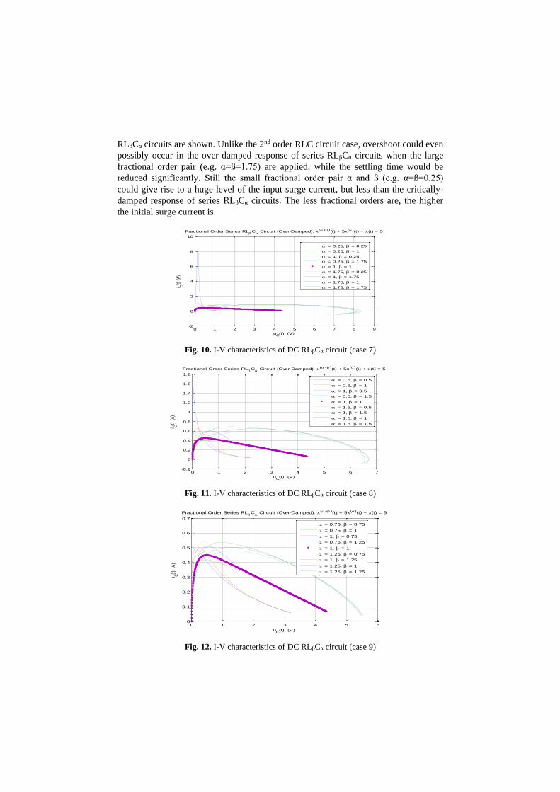
RLβCα circuits are shown. Unlike the 2nd order RLC circuit case, overshoot could even

possibly occur in the over-damped response of series RLβCα circuits when the large

fractional order pair (e.g. α=ß=1.75) are applied, while the settling time would be

reduced significantly. Still the small fractional order pair α and ß (e.g. α=ß=0.25)

could give rise to a huge level of the input surge current, but less than the critically-

damped response of series RLβCα circuits. The less fractional orders are, the higher

the initial surge current is.

0 1 2 3 4 5 6 7 8 9-2

0

2

4

6

8

10

i C(t) (

A)

uC(t) (V)

Fractional Order Series RLC Circuit (Over-Damped): x(+)(t) + 5x()(t) + x(t) = 5

= 0.25, = 0.25

= 0.25, = 1

= 1, = 0.25

= 0.25, = 1.75

= 1, = 1

= 1.75, = 0.25

= 1, = 1.75

= 1.75, = 1

= 1.75, = 1.75


0 1 2 3 4 5 6 7-0.2

0

0.2

0.4

0.6

0.8

1

1.2

1.4

1.6

1.8

i C(t) (

A)

uC(t) (V)


= 0.5, = 0.5

= 0.5, = 1

= 1, = 0.5

= 0.5, = 1.5

= 1, = 1

= 1.5, = 0.5

= 1, = 1.5

= 1.5, = 1

= 1.5, = 1.5


0 1 2 3 4 5 60

0.1

0.2

0.3

0.4

0.5

0.6

0.7

i C(t) (

A)

uC(t) (V)


= 0.75, = 0.75

= 0.75, = 1

= 1, = 0.75

= 0.75, = 1.25

= 1, = 1

= 1.25, = 0.75

= 1, = 1.25

= 1.25, = 1

= 1.25, = 1.25


5 Numerical simulations of AC series RLβCα circuits

For 2nd order AC series RLC circuits in (1-2), there are 2 dominating parameters to

manifest the behaviors: the resonant frequency and the damping ratio. The resonant

frequency is computed as (14) while the damping ratios ζS and ζP can be computed as

(15), corresponding to the 2nd order series and parallel RLC circuits respectively. The

quality factor (Q-factor) acts as a frequency-to-bandwidth (full width at half maxi-

mum) ratio of the resonator, which is relevant to the damping ratio and expressed as

(16). Generalized fractional order reactive elements are expressed as (17) and (18)

instead, representing the pseudo inductance and pseudo capacitance.

)()1/(2=)/(1/= HzLCfandsecradLC rr (14)

C

L

Rand

L

CRPS

2

1=

2= (15)

rQ =2

1= (16)

)2

(sL=)2

(/L=L 11

−−

inLandsin (17)

)2

(/C=)2

(C=C 11

−−

sinCandsin (18)

At resonance, we have (19) being satisfied. The resonant frequency of fractional

order RLβCα circuits can thus be directly computed as (20).

1=)2

(/)2

(sCL=L F

2

+ sininC O (19)

2=

/2)(sCL

/2)(s=

)(

FFO

FOO fandin

in

+

(20)

In the numerical simulations, circuit parameters being selected are similar to those

in the DC fractional order series RLβCα circuits, except for the AC power source,

where US standard AC voltage is adopted instead: ( ) ( )tcostVS 1202120= Volt.

Again to represent 3 cases of underdamping, critical-damping and overdamping of the

natural response, the resistance R has been specified as 1.0, 4.0, and 10.0 Ohm, re-

spectively. When either α=β or (α+β)=2 holds, the fractional order RLβCα circuit has

exactly the same resonant frequency as that of the typical 2nd order RLC circuit, where

the resonant angular frequency 1.0 rad/sec acts as a reference in several cases above.

The damping ratio however is defined for the 2nd order circuit exclusively. As for

potential stability control in the worst case scenario, the circuit parameters chosen in

simulations match the resonance condition, which is related to maximal amplitudes of

the AC voltage and AC current to be controlled. Fractional orders for capacitors

(0<α<2) and inductors (0<β<2) are selected as 0.25, 0.50, 0.75 1.00, 1.25, 1.50 and

1.75, respectively. Typical numerical simulation results are shown in Figs. 13-22, to

make comparisons among various characteristic curves of the AC series RLβCα cir-

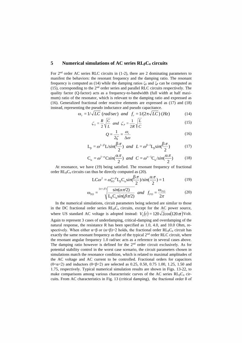
cuits. From AC characteristics in Fig. 13 (critical damping), the fractional order ß of

series RLβCα circuits has larger impact on circuit characteristics than fractional order

α, which leads to 3 distinctive characteristic curve sets significantly different from

each other. Within each of 3 sets though, the fractional order α leads to minor differ-

ences among 3 cases. Major changes of characteristic curves arise from diverse frac-

tional order ß while minor changes arise from diverse fractional order α (The role is

opposite to parallel RLβCα circuits). For both α and ß, in general, the smaller the frac-

tional order is, the earlier the time advance is and the larger the I-V characteristic

curve magnitude is (vice versa). Fractional orders α and ß will affect both the ampli-

tude and time shifting (delay or advance) in characteristic curves, covering the magni-

tude response and phase response.

0 2 4 6 8 10-25

-20

-15

-10

-5

0

5

10

15

20

25

uC(t

) (

V)

t (s)

Fractional Order Series RLC Circuit (Critically-Damped): x(+)(t) + 2x()(t) + x(t) = 1202cos(120t)

0 2 4 6 8 10-60

-40

-20

0

20

40

60

80

i C(t

) (

A)

t (s)

= 0.5, = 0.5

= 0.5, = 1

= 1, = 0.5

= 0.5, = 1.5

= 1, = 1

= 1.5, = 0.5

= 1, = 1.5

= 1.5, = 1

= 1.5, = 1.5

Fig. 13. UC(t) and i(t) of AC series RLβCα circuit (critical damping)

-200 -100 0 100 200 300 400 500 600-400

-200

0

200

400

600

800

i C(t) (

A)

uC(t) (V)

Fractional Order Series RLC Circuit (Under-Damped): x(+)(t) + 0.5x()(t) + x(t) = 1202cos(120t)

= 0.25, = 0.25

= 0.25, = 1

= 1, = 0.25

= 0.25, = 1.75

= 1, = 1

= 1.75, = 0.25

= 1, = 1.75

= 1.75, = 1

= 1.75, = 1.75

Fig. 14. I-V characteristics of AC RLβCα circuit (case 1)

-200 -150 -100 -50 0 50 100 150-150

-100

-50

0

50

100

i C(t)

(A

)

uC(t) (V)


= 0.5, = 0.5

= 0.5, = 1

= 1, = 0.5

= 0.5, = 1.5

= 1, = 1

= 1.5, = 0.5

= 1, = 1.5

= 1.5, = 1

= 1.5, = 1.5


-40 -30 -20 -10 0 10 20 30-50

-40

-30

-20

-10

0

10

20

30

40

50

i C(t)

(A

)

uC(t) (V)


= 0.75, = 0.75

= 0.75, = 1

= 1, = 0.75

= 0.75, = 1.25

= 1, = 1

= 1.25, = 0.75

= 1, = 1.25

= 1.25, = 1

= 1.25, = 1.25


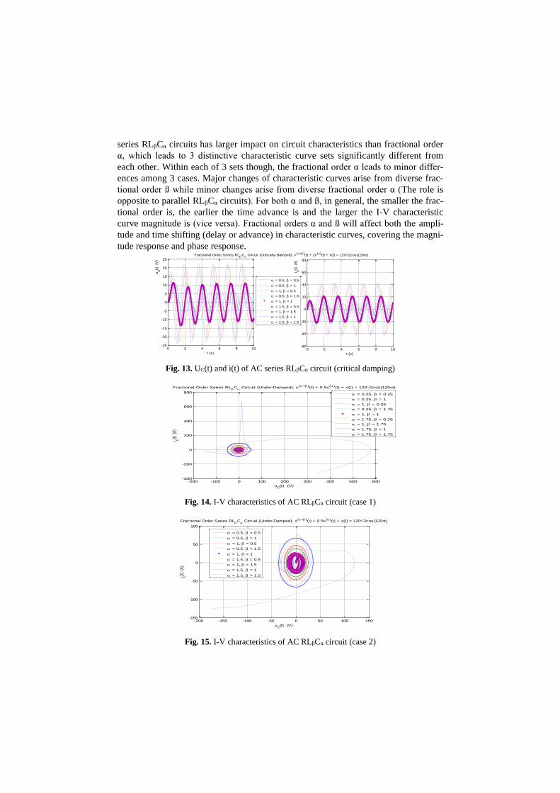
In Figs. 14-22, I-V characteristics of AC series RLβCα circuits are shown, including

all three cases of under-damping, critical-damping and over-damping, where the 2nd

order AC series RLC circuit acts as a reference (scale varies remarkably).

In Figs. 14-16, under-damped I-V characteristics (AC) are shown. The largest frac-

tional orders pair α and ß (e.g. α = ß = 1.75) could also generate increasing oscillation

for AC series RLβCα circuits. Smallest fractional orders pair α and ß (e.g. α=ß=0.25)

will generate highest level of instantaneous input surge current in the starting cycle.

The characteristic curves are significantly different from the 2nd order RLC circuits.

In Figs. 17-19, critically-damped I-V characteristics (AC) are shown. The smallest

fractional order pair α and ß (e.g. α = ß = 0.25) will generate an exceptional level of

instantaneous input surge current in the starting cycle. The smaller the fractional order

pair is, the larger the surge current is. The I-V characteristic curves will circle around

the equilibrium after initial cycles, showing behaviors of sustained oscillation.

In Figs. 20-22, over-damped I-V characteristics (AC) are shown. Still the smallest

fractional order pair α and ß (e.g. α=ß=0.25) will give rise to extra level of instantane-

ous input surge current in the starting cycle, but its impact is less than the critical-

damping case. The smaller the fractional order pair is, the larger the surge current is.

The I-V characteristic curves circle around the equilibrium after initial cycles.

-40 -30 -20 -10 0 10 20 30 40-100

0

100

200

300

400

500

i C(t

) (

A)

uC(t) (V)


= 0.25, = 0.25

= 0.25, = 1

= 1, = 0.25

= 0.25, = 1.75

= 1, = 1

= 1.75, = 0.25

= 1, = 1.75

= 1.75, = 1

= 1.75, = 1.75


-25 -20 -15 -10 -5 0 5 10 15 20 25-60

-40

-20

0

20

40

60

80

i C(t

) (

A)

uC(t) (V)


= 0.5, = 0.5

= 0.5, = 1

= 1, = 0.5

= 0.5, = 1.5

= 1, = 1

= 1.5, = 0.5

= 1, = 1.5

= 1.5, = 1

= 1.5, = 1.5


-20 -15 -10 -5 0 5 10 15 20-40

-30

-20

-10

0

10

20

30

40

i C(t

) (

A)

uC(t) (V)


= 0.75, = 0.75

= 0.75, = 1

= 1, = 0.75

= 0.75, = 1.25

= 1, = 1

= 1.25, = 0.75

= 1, = 1.25

= 1.25, = 1

= 1.25, = 1.25


-30 -20 -10 0 10 20 30-50

0

50

100

150

200

250

300

350

i C(t

) (

A)

uC(t) (V)

Fractional Order Series RLC Circuit (Over-Damped): x(+)(t) + 5x()(t) + x(t) = 1202cos(120t)

= 0.25, = 0.25

= 0.25, = 1

= 1, = 0.25

= 0.25, = 1.75

= 1, = 1

= 1.75, = 0.25

= 1, = 1.75

= 1.75, = 1

= 1.75, = 1.75


-20 -15 -10 -5 0 5 10 15 20-40

-30

-20

-10

0

10

20

30

40

50

60

i C(t

) (

A)

uC(t) (V)


= 0.5, = 0.5

= 0.5, = 1

= 1, = 0.5

= 0.5, = 1.5

= 1, = 1

= 1.5, = 0.5

= 1, = 1.5

= 1.5, = 1

= 1.5, = 1.5


-15 -10 -5 0 5 10 15-25

-20

-15

-10

-5

0

5

10

15

20

25

i C(t

) (

A)

uC(t) (V)


= 0.75, = 0.75

= 0.75, = 1

= 1, = 0.75

= 0.75, = 1.25

= 1, = 1

= 1.25, = 0.75

= 1, = 1.25

= 1.25, = 1

= 1.25, = 1.25


6 Conclusion

The fractional order RLβCα circuit has been analyzed in this preliminary study. It can

deliver more flexibility for potential stability control and performance enhancement

than the 2nd order RLC circuits. The series fractional order RLβCα circuit is applied as

the example for characteristic analysis where the fractional Riemann-Liouville deriva-

tives are applied. Various DC and AC circuit cases with different fractional order pair

α and β are taken into account for comparison purposes. The stability issue has been

the focus of the DC fractional order RLβCα circuit through the step response analysis.

The magnitude transient response (magnitude) and time shifting (phase) are both em-

phasized in AC fractional order RLβCα circuit analysis at the resonant frequency. I-V

characteristics are presented on all three cases of underdamping, critical-damping and

overdamping via numerical simulations. It shows that the fractional order β has great-

er impact than fractional order α on characteristics of series fractional order RLβCα

circuits in general, no matter if the DC or AC circuit is applied. The large pair of the

fractional order α and β takes the leading role in system stability, while the small pair

of the fractional order α and β has negative influence in the instantaneous input surge

current at the starting stage. This research work has provided the useful insights into

the potential stability problems in numerous engineering applications such as dynamic

control, robotics, mechatronics and communication.

References

1. Gutiérrez R., Rosário J., and Tenreiro J.: Fractional order calculus: basic concepts and en-

gineering applications. Mathematical Problems in Engineering Journal, pp. 1-19 (2010)

2. Ye Z.: "Modeling, identification, design and implementation of nonlinear automotive idle

speed control systems - an overview", IEEE Transactions on Systems, Man and Cybernet-

ics, Part C: Applications and Reviews, Vol. 37, No. 6, pp. 1137-1151 (2007)

3. Ye Z., Mohamadian H., and Yin H.: Impact of fractional orders on characteristics of chaot-

ic dynamical systems. International Journal of Electrical, Electronics and Data Communi-

cation, Vol. 5, Issue 2, pp. 72-77 (2017)

4. Tsirimokou G., Psychalinos C., Elwakil A., and Salama K: Electronically tunable fully in-

tegrated fractional-order resonator. IEEE Transactions on Circuits and Systems II: Express

Briefs, Vol. 65, No. 2, pp. 166-170 (2018)

5. Ye Z., Yin H., and Meng A.: Comparative studies of DC motor FOPID control with opti-

mal state estimation using kalman filter. In Proceedings of International Conference on

Power Electronics and Their Applications, September 25-27, Elazig, Turkey (2019)

6. Ye Z., and Mohamadian H.: Application of modern control theory on performance analysis

of generalized notch filters. In Proceedings of International Conference on Modern Cir-

cuits and Systems Technologies, May 12-14, 2016, Thessaloniki, Greece (2016)

7. Ye Z., and Mohamadian H.: Comparative study of generalized electrical and optical notch

filters via classical control theory. In Proceedings of International Conference on Modern

Circuits and Systems Technologies, May 12-14, Thessaloniki, Greece (2016)

8. Zhang G., Ou Z., and Qu L.: A fractional-order element based approach to wireless power

transmission for frequency reduction and output power quality improvement. MDPI Jour-

nal of Electronics, Vol. 8, pp. 14 (2019)

9. Dimeas I., Tsirimokou G., Psychalinos C. and Elwakil A.: Realization of fractional-order

capacitor and inductor emulators using current feedback operational amplifiers. In Pro-

ceedings of International Symposium on Nonlinear Theory and its Applications, December

1-4, 2015, Kowloon, Hong Kong, China, pp. 237-240 (2015)

10. Gomez F., Rosales J., and Guia M.: RLC electrical circuit of non-integer order. Central

European Journal of Physics, Vol. 11, No. 10, pp. 1361-1365 (2013)

11. Stankiewicz A.: Fractional order RLC circuits. In Proceedings of 2017 International Con-

ference on Electromagnetic Devices and Processes in Environment Protection with Semi-

nar Applications of Superconductors, pp. 4, December 3-6, 2017, Lublin, Poland (2017)

12. Alsaedi A., Nieto J., and Venktesh V.: Fractional electrical circuits. Advances in Mechani-

cal Engineering Journal, Vol. 7 (12), pp. 1–7 (2015)

13. Walczak J., Jakubowska A.: Resonance in series fractional order RLβCα circuit. Przegląd

Elektrotechniczny, R. 90, No. 4, pp. 210-213 (2014)

characteristic analysis of dc and ac fractional order rl c

Documents