a characteristic difference method for fractional ...ashm-journal.com/test/vol3-1/72.pdf · applied...
TRANSCRIPT
Applied mathematics in Engineering, Management and Technology 3(1) 2015:618-630
www.amiemt-journal.com
618
Abstract
In this paper, Fractional advection-dispersion equations, which is important in
modeling the transport of passive tracers carried by fluid flow in a porous medium, is
revisited. It is applied a technique so-called characteristic finite difference method
(CFDM) to analyze 2-D fractional advection-dispersion equations with variable
coefficients on a finite domain. This method is in fact the combination of
characteristic methods and fractional finite difference techniques. Also, stability,
consistency and convergence of CFDM are fully discussed and more, an error
estimate is given. Furthermore, some numerical illustrative examples are carried out
and compared with other known methods.
Key words:Finite difference approximation; Radial dispersion; Shifted Grünwald-Letnikov
formula; Method of characteristics; Fractional advection-dispersion.
1. Introduction and basic formulation
The history of fractional calculus and integer-order calculus is almost the same [1, 2]. However, fractional
calculus was not developed very fast in comparison to integer-order calculus until the late 1970s due to lack of
application background. Since then, it has progressively found applications in many different fields of
engineering and sciences. For instance, fractional derivatives have recently been applied to some problems in
physics [3, 4, 5, 6, 7, 8, 9, 10, 11, 12, 13, 14, 15], finance [16, 17, 18] and hydrology [19, 20, 21, 22, 23, 24, 25,
26]. Fractional space derivatives usually are used to model anomalous diffusion or dispersion. When second
derivative in a diffusion or dispersion model is replaced by a fractional derivative, it leads to superdiffusion or
enhanced diffusion. When one dimensional advection-dispersion model has constant coefficients, analytical
solutions can be obtained by using Fourier transform methods [7, 21]. However, many practical problems lead to
a model with variable coefficients [4, 27].
In current paper, we develop the basic theory of characteristic finite difference method (CFDM) for the
space-fractional advection-dispersion equation
∂𝑢(𝑥 ,𝑡)
∂𝑡 + 𝑉(𝑥, 𝑡)
∂𝑢(𝑥 ,𝑡)
∂𝑥 − 𝐷 (𝑥, 𝑡)
∂𝛼𝑢(𝑥 ,𝑡)
∂𝑥𝛼 = 𝑠(𝑥, 𝑡) (1)
on a finite domain 𝑥𝐿 < 𝑥 < 𝑥𝑅. Physical considerations need 1 < 𝛼 ≤ 2 , see [25]. We suppose 𝑉(𝑥, 𝑡) ≥ 0
and 𝐷(𝑥, 𝑡) ≥ 0 so that the flow is from left to right. We also suppose an initial condition 𝑢(𝑥, 0) = 𝑢0(𝑥) for
𝑥𝐿 < 𝑥 < 𝑥𝑅 and a natural set of boundary conditions for mentioned problem: 𝑢(𝑥𝐿 , 𝑡) = 0 for all 𝑡 ≥ 0 and ∂𝑢(𝑥𝑅 ,𝑡)
∂𝑡= 0 for all 𝑡 ≥ 0. From the physical point of view, the boundary conditions mean that no tracer leaks
past the left boundary, and that the tracer moves freely through the right boundary. With these assumptions, it has
been shown in [28] that the implicit Euler method is unconditionally stable when a modified form of the
Grünwald formula is used for the fractional derivative. Otherwise, the implicit Euler method is unstable and so its
solution does not converge to the exact solution. The explicit Euler method is unstable as well when the standard
Grünwald formula is used. The term ∂𝛼𝑢(𝑥 ,𝑡)
∂𝑥𝛼 in Eq.(1) is the Riemann-Liouville fractional derivative of order 𝛼,
which is defined by
A characteristic difference method for fractional
advection-dispersion flow equations
Elyas Shivanian*, Hamid Reza Khodabandehlo
Department of Mathematics, Imam Khomeini International University, Qazvin, 34149-16818, Iran
Applied mathematics in Engineering, Management and Technology 3(1) 2015:618-630
www.amiemt-journal.com
619
∂𝛼𝑓(𝑥)
∂𝑥𝛼 =
1
Γ(𝑛−𝛼)
𝑑𝑛
𝑑𝑥𝑛 𝑥
𝑥𝐿
𝑓(𝜉)
(𝑥−𝜉)𝛼+1−𝑛 𝑑𝜉 , (2)
where 𝑛 is an integer such that 𝑛 − 1 < 𝛼 ≤ 𝑛 and Γ(. ) is the well known Gamma function. In most of the
related literature, the case 𝑥𝐿 = 0 is called the Riemann-Liouville form, and the case 𝑥𝐿 = −∞ is called the
Liouville definition. Since 1 < 𝛼 ≤ 2 then
∂𝛼𝑓(𝑥)
∂𝑥𝛼 =
1
Γ(2−𝛼)
𝑑2
𝑑𝑥2 𝑥
𝑥𝐿
𝑓(𝜉)
(𝑥−𝜉)𝛼−1 𝑑𝜉. (3)
The Grünwald-Letnikov definition of fractional derivatives of order 𝛼 of a function 𝑓(𝑥) for 𝑥∈ ∈ [𝑥𝐿 ,𝑥𝑅]
is probably more computationally feasible, which are defined by [29]
∂𝛼𝑓(𝑥)
∂𝑥𝛼 = lim
→ 0
1
𝛼
[𝑥−𝑥𝐿
]
𝑘=0 𝑔𝑘(𝛼)
𝑓(𝑥 − 𝑘), (4)
where is the space step and 𝑔𝑘(𝛼)
= (−1)𝑘 𝛼𝑘 =
Γ(𝑘 − 𝛼)
Γ(− 𝛼) Γ(𝑘 + 1) with
𝛼𝑘 being the binomial
coefficients.
The Riemann-Liouville definition and the Grünwald-Letnikov definition coincide under relatively weak
conditions [30]: If 𝑓(𝑥) has second-order Sobolev derivative on the interval [𝑥𝐿 ,𝑥𝑅], then for every 1 < 𝛼 ≤ 2
both the Riemann-Liouville and the Grünwald-Letnikov derivatives exist and coincide on the interval [𝑥𝐿 ,𝑥𝑅].
This equivalence enables us to use the computationally more feasible Grünwald-Letnikov definition (4) in the
numerical discretization. The following shifted Grünwald approximations in discrete forms at each node 𝑥 were
introduced in [31]
∂𝛼𝑓(𝑥)
∂𝑥𝛼 =
1
𝛼
[𝑙1] + 1𝑘=0 𝑔𝑘
(𝛼) 𝑓(𝑥 − (𝑘 − 1)) + 𝑎1
∂𝛼+1𝑓(𝑥)
∂𝑥𝛼+1 + 𝑂(2), (5)
where 𝑙1 = (𝑥−𝑥𝐿)
, with [𝑙1] being the floor of 𝑙1 , respectively. The constants 𝑎1 is independent of ,𝑓 and
𝑥 . Moreover, the coefficients 𝑔𝑘(𝛼)
can be evaluated recursively:
𝑔0(𝛼)
= 1 , 𝑔𝑘(𝛼)
= (1 − 𝛼+1
𝑘) 𝑔𝑘−1
(𝛼). (6)
2. A fractional characteristic finite difference method
In this section, we develop a fractional characteristic finite difference method [32, 33] for problem (1) base upon
the Eulerian fractional finite difference method for problem (1) with the characteristic method which has been
well developed for second-order transient advection-diffusion equations [34]. Let 𝜓(𝑥, 𝑡) = 1 + 𝑉2(𝑥, 𝑡)
and denote the characteristic direction associated with the operator 𝑢𝑡 + 𝑉(𝑥, 𝑡) 𝑢𝑥 , by 𝜏 = 𝜏(𝑥, 𝑡) , then the
derivative along the characteristic direction can be written as [34]
𝑑
𝑑𝜏 =
1
𝜓(𝑥 ,𝑡) ∂
∂𝑡 +
𝑉(𝑥 ,𝑡)
𝜓(𝑥 ,𝑡) ∂
∂𝑥,
and the hyperbolic part of Eq.(1) becomes
∂𝑢 (𝑥 ,𝑡)
∂𝑡 + 𝑉(𝑥, 𝑡)
∂𝑢 (𝑥 ,𝑡)
∂𝑥 = 𝜓(𝑥, 𝑡)
𝑑𝑢 (𝑥 ,𝑡)
𝑑𝜏.
Thus, the fractional advection-diffusion equation in (1) is rewritten as a fractional parabolic equation along the
characteristics
𝜓(𝑥, 𝑡) 𝑑𝑢 (𝑥 ,𝑡)
𝑑𝜏 − 𝐷 (𝑥, 𝑡)
∂𝛼𝑢(𝑥 ,𝑡)
∂𝑥𝛼 = 𝑠(𝑥, 𝑡), (7)
In other words, the nonsymmetry due to advection in the governing fractional advection-diffusion equation (1) is
symmetrized in (7) in the Lagrangian coordinates. Let 𝑀 be a positive integer and Δ𝑡 = 𝑇
𝑀. We define a
uniform partition of the time interval [ 0 ,𝑇 ] by 𝑡𝑚 . For any 𝑥 ∈ [𝑥𝐿 ,𝑥𝑅] at time step 𝑡𝑚+1, we define a
backward characteristic tracking by
𝑟(𝑡; 𝑥, 𝑡𝑚+1) = 𝑥 − 𝑉(𝑥, 𝑡𝑚 + 1) (𝑡𝑚+1 − 𝑡),
𝑥 = 𝑟(𝑡𝑚 ; 𝑥, 𝑡𝑚+1) = 𝑥 − 𝑉(𝑥, 𝑡𝑚+1) Δ𝑡,
Δ𝑡 = 𝑡𝑚+1 − 𝑡𝑚 .
(8)
Applied mathematics in Engineering, Management and Technology 3(1) 2015:618-630
www.amiemt-journal.com
620
Then the characteristic derivative is approximated by a backward difference quotient along the approximate
characteristics (8) in the time stepping procedure [34]
𝜓(𝑥, 𝑡𝑚+1) 𝑑𝑢 (𝑥 ,𝑡𝑚+1)
𝑑𝜏 = 𝜓(𝑥, 𝑡𝑚+1)
𝑢(𝑥 ,𝑡𝑚+1) − 𝑢(𝑥 ,𝑡𝑚 )
(𝑥 − 𝑥)2 +(Δ𝑡)2 + 𝑅(1)(𝑥, 𝑡𝑚+1)
= 𝜓(𝑥, 𝑡𝑚+1) 𝑢(𝑥 ,𝑡𝑚+1) − 𝑢(𝑥 ,𝑡𝑚 )
(𝑥 − 𝑥 +𝑉(𝑥 ,𝑡𝑚+1) Δ𝑡)2 +(Δ𝑡)2 + 𝑅(1)(𝑥, 𝑡𝑚+1)
= 𝜓(𝑥, 𝑡𝑚+1) 𝑢(𝑥 ,𝑡𝑚+1) − 𝑢(𝑥 ,𝑡𝑚 )
(𝑉2(𝑥 ,𝑡𝑚+1) +1)(Δ𝑡)2 + 𝑅(1)(𝑥, 𝑡𝑚+1)
= 𝜓(𝑥, 𝑡𝑚+1) 𝑢(𝑥 ,𝑡𝑚+1) − 𝑢(𝑥 ,𝑡𝑚 )
𝜓(𝑥 ,𝑡𝑚+1)Δ𝑡 + 𝑅(1)(𝑥, 𝑡𝑚+1)
= 𝑢(𝑥 ,𝑡𝑚+1) − 𝑢(𝑥 ,𝑡𝑚 )
Δ𝑡 + 𝑅(1)(𝑥, 𝑡𝑚+1)
(9)
where 𝑅(1)(𝑥, 𝑡𝑚+1) is the local truncation error defined by
𝑅(1)(𝑥, 𝑡𝑚+1) = 1
Δ𝑡 𝑡𝑚+1
𝑡𝑚 (𝑟(𝑡; 𝑥, 𝑡𝑚+1) − 𝑥)2 + (𝑡 − 𝑡𝑚 )2 𝑑2 𝑢
𝑑𝜏2 (𝑟(𝑡; 𝑥, 𝑡𝑚+1), 𝑡) 𝑑𝜏
= 1
Δ𝑡 𝑡𝑚+1
𝑡𝑚 ((𝑥 − 𝑉(𝑥, 𝑡𝑚+1))(𝑡𝑚 − 𝑡) − 𝑥 + 𝑉(𝑥, 𝑡𝑚+1)Δ𝑡)2 + (𝑡 − 𝑡𝑚 )2 𝑑2 𝑢
𝑑𝜏2 (𝑟(𝑡; 𝑥, 𝑡𝑚+1), 𝑡)𝑑𝜏
= 1
Δ𝑡 𝑡𝑚+1
𝑡𝑚 𝑉2(𝑥, 𝑡𝑚+1)(Δ𝑡 − (𝑡𝑚+1 − 𝑡))2 + (𝑡 − 𝑡𝑚 )2 𝑑2 𝑢
𝑑𝜏2 (𝑟(𝑡; 𝑥, 𝑡𝑚+1), 𝑡) 𝑑𝜏
= 1
Δ𝑡 𝑡𝑚+1
𝑡𝑚 (𝑉2(𝑥, 𝑡𝑚+1) + 1) (𝑡 − 𝑡𝑚 )2 𝑑2 𝑢
𝑑𝜏2 (𝑟(𝑡; 𝑥, 𝑡𝑚+1), 𝑡) 𝑑𝜏
= 1
Δ𝑡 𝑡𝑚+1
𝑡𝑚 (𝑉2(𝑥, 𝑡𝑚+1) + 1) (𝑡 − 𝑡𝑚 )
𝑑2 𝑢
𝑑𝜏2 (𝑟(𝑡; 𝑥, 𝑡𝑚+1), 𝑡) 𝑑𝜏.
(10)
Then a semi-discrete form of Eq.(7) can be written as
𝑢(𝑥 ,𝑡𝑚+1) − 𝑢(𝑥 ,𝑡𝑚 )
Δ𝑡 − 𝐷 (𝑥, 𝑡𝑚+1)
∂𝛼𝑢(𝑥 ,𝑡𝑚+1)
∂𝑥𝛼 = 𝑠(𝑥, 𝑡𝑚+1) − 𝑅(1)(𝑥, 𝑡𝑚+1). (11)
To develop a characteristic finite difference method, we are now in a position to discretize the fractional
diffusion terms. At each node 𝑥𝑖 = 𝑥𝐿 + 𝑖 for 𝑖 = 1,2, . . . ,𝑁 − 1 with = (𝑥𝑅 − 𝑥𝐿)
𝑁, we use the first-order
shifted Grünwald approximations (5) to discretize the fractional diffusion term as follows [31]
∂𝛼𝑢(𝑥𝑖 ,𝑡
𝑚+1)
∂+𝑥𝛼 =
1
𝛼 𝑖 + 1𝑘=0 𝑔𝑘
(𝛼) 𝑢(𝑥𝑖 −𝑘 +1, 𝑡𝑚+1) + 𝑅+
(2)(𝑥𝑖 , 𝑡
𝑚+1), (12)
where 𝑅+(2)
(𝑥𝑖 , 𝑡𝑚+1) is local truncation term of order 𝑂() defined by
𝑅+(2)
(𝑥𝑖 , 𝑡𝑚+1) = 𝑎1
∂𝛼+1𝑢(𝑥𝑖 ,𝑡𝑚+1)
∂+𝑥𝛼+1 + 𝑂(2). (13)
Then the semi-discrete form (11) of Eq.(1) can be written as the following fully discrete form
𝑢(𝑥𝑖 ,𝑡
𝑚+1) − 𝑢(𝑥𝑖 ,𝑡𝑚 )
Δ𝑡 −
𝐷 (𝑥 ,𝑡𝑚+1)
𝛼 𝑖 + 1𝑘=0 𝑔𝑘
(𝛼) 𝑢(𝑥𝑖 −𝑘 +1 , 𝑡𝑚+1) = 𝑠(𝑥𝑖 , 𝑡
𝑚+1) − 𝑅(𝑥𝑖 , 𝑡𝑚+1), (14)
where 𝑅(𝑥𝑖 , 𝑡𝑚+1) is the local truncation error defined by
𝑅(𝑥𝑖 , 𝑡𝑚+1) = − 𝑅(1)(𝑥𝑖 , 𝑡
𝑚+1) + 𝐷 (𝑥, 𝑡𝑚+1) 𝑅+(2)
(𝑥𝑖 , 𝑡𝑚+1). (15)
We let the node functions 𝑈𝑖𝑚 be the numerical approximation to the true solution 𝑢(𝑥𝑖 , 𝑡
𝑚 ) , 𝑉𝑖𝑚 =
𝑉(𝑥𝑖 , 𝑡𝑚 ), 𝑠𝑖
𝑚 = 𝑠(𝑥𝑖 , 𝑡𝑚 ) , 𝐷𝑖
𝑚 = 𝐷(𝑥(𝑖), 𝑡𝑚 ). The characteristic finite difference method for problem (1)) is
formulated as follows: At each time step 𝑡𝑚+1, find 𝑈𝑖𝑚+1 for 𝑖 = 1,2, . . . ,𝑁 − 1 such that
𝑈𝑖𝑚+1 − 𝑈𝑖
𝑚+1
Δ𝑡 −
𝐷 𝑚+1
𝛼 𝑖 + 1𝑘=0 𝑔𝑘
(𝛼) 𝑈𝑖 −𝑘 +1
𝑚+1 = 𝑠𝑖𝑚+1 . (16)
Applied mathematics in Engineering, Management and Technology 3(1) 2015:618-630
www.amiemt-journal.com
621
Note that in general 𝑥𝑖 does not necessarily coincide with a node in the space, so 𝑈𝑖𝑚
is not defined. In this
case, 𝑈𝑖𝑚
can be evaluated via a linear interpolation. More specifically, let 𝐶𝑟𝑖 = 𝑉𝑖𝑚
Δ𝑡
𝑡 be the Courant
number and [ 𝐶𝑟𝑖] be its floor. When the Courant number 𝐶𝑟𝑖 is an integer, 𝑥𝑖 will intersect a node at time
step 𝑡𝑚 , so the evaluation of 𝑈𝑖𝑚
is straightforward. Otherwise, 𝑥𝑖 falls into the interval [𝑥𝑖0𝑚 , 𝑥𝑖0𝑚 +1] where
𝑖0𝑚 = 𝑖𝑚 − [𝐶𝑟𝑖] − 1.
Thus, 𝑈𝑖𝑚
can be evaluated by
𝑈𝑖𝑚
= (1 − 𝐶𝑟𝑖𝑚 ,∗ )𝑈𝑖0𝑚 +1 + 𝐶𝑟𝑖
𝑚 ,∗ 𝑈𝑖0𝑚𝑚 + 𝑂(2), (17)
with 𝐶𝑟𝑖𝑚 ,∗ being the fractional part of the Courant number. In practice, the diffusion is often symmetric.
In this case, the characteristic finite difference scheme (16) symmetrizes the governing fractional
advection-diffusion equations and generates a symmetric and positive-definite coefficient matrix with a greatly
improved, almost well conditioned number. In contrast, the fractional finite difference methods with standard
temporal discretization tend to generate nonsymmetric and ill-conditioned coefficient matrices.
3. Stability and error analysis of the fractional characteristic finite difference method
In this section we analyze the stability and convergence behavior of the characteristic finite difference method.
3.1. Three useful lemmas
For the purpose of the analysis, we rewrite the numerical scheme (16) into the following form
𝑈𝑖𝑚+1 − 𝜉𝑚+1 𝑖 +1
𝑘=0 𝑔𝑘(𝛼)
𝑈𝑖 −𝑘 +1𝑚+1 = (1 − 𝐶𝑟𝑖
𝑚 ,∗ )𝑈𝑖0𝑚 +1 + 𝐶𝑟𝑖𝑚 ,∗ 𝑈𝑖0𝑚
𝑚 + Δ𝑡𝑠𝑖𝑚+1 ,
𝑖 = 1,2, . . . ,𝑁 − 1 ,𝑚 = 0,1, . . . ,𝑀 − 1 ,
𝑈𝑖0 = 𝑈0(𝑥𝑖) , 𝑖 = 1,2, . . . ,𝑁 − 1,
(18)
where 𝜉𝑖𝑚+1 = 𝐷𝑖
𝑚+1 Δ𝑡
𝛼 are associated with the diffusion coefficients. We carry out the analysis via the
approach of matrix analysis. To do so, we first recall some basic concepts in the theory of matrix analysis. The
following two lemmas play an important role in the analysis [35, 36]:
Lemma 3.1 Assume A = [ai,j] is diagonally dominant by rows. Then, the following estimate holds
∥ A ∥∞ ≤ max1 ≤ i ≤ n
1
|ai ,j | − 1≤j≤n ,j≠i |ai ,j |. (19)
Lemma 3.2 The coefficients gk(α)
given in (6) with 1 < α „ 2 satisfy the following properties:
g0
(α) = 1 , g1
(α) = − α < 0,
1 ≥ g2(α)
≥ g3(α)
≥ . . .≥ 0
∞k = 0 gk
(α) = 0 ,
mk = 0 gk
(α) ≤ 0 , (m ≥ 1).
(20)
To proving lemma(3.2) it is enough present following lemma that was proved in [28].
Lemma 3.3 It is well known that
( 1 + z)α = ∞k = 0
kα zk ,
for any complex |z| ≤ 1 and any α ≥ 0 , where
kα =
(−1)α Γ(k − α)
Γ( − α) Γ(k + 1),

Applied mathematics in Engineering, Management and Technology 3(1) 2015:618-630
www.amiemt-journal.com
622
kα (−1)k =
(−α) (−α +1) ...(−α + k − 1)
k! =
Γ(k − α)
Γ( − α) Γ(k + 1) .
3.2. Stability analysis
Theorem 3.4 The characteristic finite difference scheme (16) is unconditionally stable in the L∞ norm for
1 < α „ 2 . In particular, the matrices Am+1 and Bm defined in (23)-(25) below satisfy
∥ (Am+1)−1 Bm ∥∞≤ 1, ∥ (Am+1)−1 ∥∞≤ 1. (21)
Proof. We notice that the scheme (18) can be written as a matrix form
𝐴𝑚+1 𝑈𝑚+1 = 𝐵𝑚 𝑈𝑚 + Δ𝑡 𝑆𝑚+1 , 𝑚 = 0,1, . . . ,𝑀 − 1. (22)
Here
𝑈𝑚 = [𝑈1𝑚 ,𝑈1
𝑚 , . . . ,𝑈1𝑚 ]𝑇 , 𝑆𝑚 = [𝑆1
𝑚 ,𝑆2𝑚 , . . . , 𝑆𝑁−1
𝑚 ]𝑇 ,
𝐴𝑚+1 = [𝑎𝑖,𝑗𝑚+1]𝑖 ,𝑗 =1
𝑁−1 ,𝐵𝑚 = [𝑏𝑖,𝑗𝑚 ]𝑖 ,𝑗 =1
𝑁−1 , (23)
with
𝑎𝑖 ,𝑗𝑚+1 =
1 − 𝜉𝑖
𝑚+1 𝑔1(𝛼)
, 𝑗 = 𝑖,
− 𝜉𝑖𝑚+1 𝑔2
(𝛼), 𝑗 = 𝑖 − 1,
− 𝜉𝑖𝑚+1 𝑔0, 𝑗 = 𝑖 + 1,
− 𝜉𝑖𝑚+1 𝑔𝑖 −𝑗 +1
(𝛼), 𝑗 < 𝑖 − 1,
0, 𝑗 > 𝑖 + 1,
(24)
𝑏𝑖,𝑗𝑚 =
1 − 𝐶𝑟𝑖𝑚 ,∗, 𝑗 = 𝑖 − [𝐶𝑟𝑖] ,
𝐶𝑟𝑖𝑚 ,∗, 𝑗 = 𝑖 − [𝐶𝑟𝑖] − 1,
0, 𝑜𝑡𝑒𝑟𝑤𝑖𝑠𝑒.
(25)
It is clear that 𝐵𝑚 ≥ 0 elementwise. Furthermore, obviously we have
∥ 𝐵𝑚 ∥∞ = max1 ≤ 𝑖 ≤ 𝑁−1
𝑁−1𝑗 = 1 |𝑏𝑖,𝑗
𝑚 | ≤ 1. (26)
As for matrix 𝐴𝑚+1 , we use Lemma (3.2) to conclude that 𝑎𝑖,𝑗𝑚+1 ≤ 0 for all 𝑖 ≠ 𝑗 , and
𝑎𝑖 ,𝑖𝑚+1 = 1 − 𝜉𝑖
𝑚+1 𝑔1(𝛼)
= 1 + 𝜉𝑖𝑚+1 𝛼 > 0. (27)
Thus, we have
𝑁−1𝑗 = 1,𝑖≠𝑗 |𝑎𝑖 ,𝑗
𝑚+1| = 𝜉𝑖𝑚+1 𝑖
𝑘=0,𝑘≠ 1 𝑔𝑘(𝛼)
≤ 𝜉𝑖𝑚+1 𝛼. (28)
We combine (27) and (28) to obtain
|𝑎𝑖 ,𝑖𝑚+1| − 𝑁−1
𝑗 = 1,𝑖≠𝑗 |𝑎𝑖 ,𝑗𝑚+1| ≥ 1. (29)
So, 𝐴𝑚+1 is diagonally dominant by rows, and from Lemma (3.1) we have
∥ (𝐴𝑚+1)−1 ∥∞ ≤ max1 ≤ 𝑖 ≤ 𝑁−1
1
|𝑎𝑖,𝑗𝑚+1| − 1≤𝑗≤𝑁−1 ,𝑗≠𝑖 |𝑎𝑖,𝑗
𝑚+1| = 1. (30)
Thus, the second estimate of (21) is proved.
Finally, we combine (26) with (30) to conclude
∥ (𝐴𝑚+1)−1 𝐵𝑚 ∥∞ ≤ ∥ (𝐴𝑚+1)−1 ∥∞ ∥ 𝐵𝑚 ∥∞ ≤ 1. (31)
Therefore, we have proved the first estimate in (4.4). This concludes the proof.
4. Convergence analysis and error estimates
Let 𝑊∞𝑘 (𝑥𝐿 ,𝑥𝑅) be the Sobolev spaces defined by [37]
𝑊∞𝑘 (𝑥𝐿 ,𝑥𝑅) = 𝑓(𝑥) ∈ 𝐿∞(𝑥𝐿 ,𝑥𝑅) ;
𝑑𝑚 𝑓(𝑥)
𝑑𝑥𝑚 ∈ 𝐿∞(𝑥𝐿 ,𝑥𝑅) , 0 ≤ 𝑚 ≤ 𝑘 , (32)
with the norm given by
Applied mathematics in Engineering, Management and Technology 3(1) 2015:618-630
www.amiemt-journal.com
623
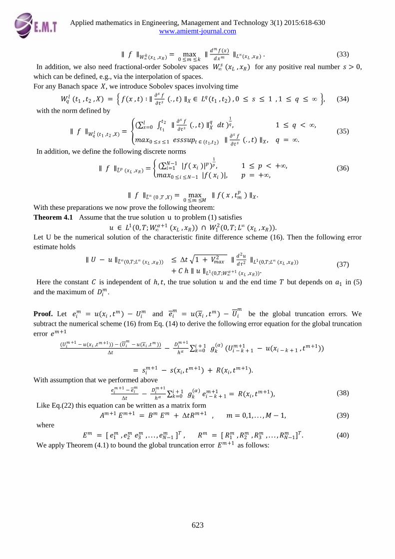
∥ 𝑓 ∥𝑊∞𝑘(𝑥𝐿 ,𝑥𝑅) = max
0 ≤ 𝑚 ≤ 𝑘 ∥
𝑑𝑚 𝑓(𝑥)
𝑑𝑥𝑚 ∥𝐿∞(𝑥𝐿 ,𝑥𝑅) . (33)
In addition, we also need fractional-order Sobolev spaces 𝑊∞𝑠 (𝑥𝐿 ,𝑥𝑅) for any positive real number 𝑠 > 0,
which can be defined, e.g., via the interpolation of spaces.
For any Banach space 𝑋, we introduce Sobolev spaces involving time
𝑊𝑞𝑙 (𝑡1 , 𝑡2 ,𝑋) = 𝑓(𝑥 , 𝑡) ∶ ∥
∂𝑠 𝑓
∂𝑡𝑠 (. , 𝑡) ∥𝑋 ∈ 𝐿𝑞(𝑡1 , 𝑡2) , 0 ≤ 𝑠 ≤ 1 , 1 ≤ 𝑞 ≤ ∞ , (34)
with the norm defined by
∥ 𝑓 ∥𝑊𝑞𝑙 (𝑡1 ,𝑡2 ,𝑋) =
( 𝑙𝑠=0
𝑡2
𝑡1 ∥
∂𝑠 𝑓
∂𝑡𝑠 (. , 𝑡) ∥𝑋
𝑞 𝑑𝑡 )
1
𝑞 , 1 ≤ 𝑞 < ∞,
𝑚𝑎𝑥0 ≤ 𝑠 ≤ 1 𝑒𝑠𝑠𝑠𝑢𝑝𝑡 ∈ (𝑡1 ,𝑡2) ∥∂𝑠 𝑓
∂𝑡 𝑠 (. , 𝑡) ∥𝑋 , 𝑞 = ∞.
(35)
In addition, we define the following discrete norms
∥ 𝑓 ∥𝐿 𝑝 (𝑥𝐿 ,𝑥𝑅) = ( 𝑁−1𝑖=1 |𝑓( 𝑥𝑖 )|𝑝)
1
𝑝 , 1 ≤ 𝑝 < +∞,
𝑚𝑎𝑥0 ≤ 𝑖 ≤ 𝑁−1 |𝑓( 𝑥𝑖 )|, 𝑝 = +∞, (36)
∥ 𝑓 ∥𝐿 ∞ (0 ,𝑇 ,𝑋) = max0 ≤ 𝑚 ≤𝑀
∥ 𝑓( 𝑥 , 𝑡𝑚𝑝
) ∥𝑋 .
With these preparations we now prove the following theorem:
Theorem 4.1 Assume that the true solution u to problem (1) satisfies
𝑢 ∈ 𝐿1(0,𝑇;𝑊∞𝛼+1 (𝑥𝐿 , 𝑥𝑅)) ∩ 𝑊1
2(0,𝑇; 𝐿∞ (𝑥𝐿 ,𝑥𝑅)).
Let U be the numerical solution of the characteristic finite difference scheme (16). Then the following error
estimate holds
∥ 𝑈 − 𝑢 ∥𝐿 ∞(0,𝑇;𝐿∞ (𝑥𝐿 ,𝑥𝑅)) ≤ Δ𝑡 1 + 𝑉𝑚𝑎𝑥
2 ∥𝑑2𝑢
𝑑𝜏2 ∥𝐿1(0,𝑇;𝐿∞ (𝑥𝐿 ,𝑥𝑅))
+ 𝐶 ∥ 𝑢 ∥𝐿1(0,𝑇;𝑊∞𝛼+1 (𝑥𝐿 ,𝑥𝑅)).
(37)
Here the constant 𝐶 is independent of , 𝑡, the true solution 𝑢 and the end time 𝑇 but depends on 𝑎1 in (5)
and the maximum of 𝐷𝑖𝑚 .
Proof. Let 𝑒𝑖𝑚 = 𝑢(𝑥𝑖 , 𝑡
𝑚 ) − 𝑈𝑖𝑚 and 𝑒𝑖
𝑚 = 𝑢(𝑥𝑖 , 𝑡
𝑚 ) − 𝑈𝑖𝑚
be the global truncation errors. We
subtract the numerical scheme (16) from Eq. (14) to derive the following error equation for the global truncation
error 𝑒𝑚+1
(𝑈𝑖
𝑚+1 − 𝑢(𝑥𝑖 ,𝑡𝑚+1)) − (𝑈𝑖
𝑚 − 𝑢(𝑥𝑖 ,𝑡
𝑚 ))
Δ𝑡 −
𝐷𝑖𝑚+1
𝛼 𝑖 + 1𝑘=0 𝑔𝑘
(𝛼) (𝑈𝑖 − 𝑘 + 1
𝑚+1 − 𝑢(𝑥𝑖 − 𝑘 + 1 , 𝑡𝑚+1))
= 𝑠𝑖𝑚+1 − 𝑠(𝑥𝑖 , 𝑡
𝑚+1) + 𝑅(𝑥𝑖 , 𝑡𝑚+1).
With assumption that we performed above
𝑒𝑖𝑚+1 − 𝑒𝑖
𝑚
Δ𝑡 −
𝐷𝑖𝑚+1
𝛼 𝑖 + 1𝑘=0 𝑔𝑘
(𝛼) 𝑒𝑖 − 𝑘 + 1𝑚+1 = 𝑅(𝑥𝑖 , 𝑡
𝑚+1), (38)
Like Eq.(22) this equation can be written as a matrix form
𝐴𝑚+1 𝐸𝑚+1 = 𝐵𝑚 𝐸𝑚 + Δ𝑡𝑅𝑚+1 , 𝑚 = 0,1, . . . ,𝑀− 1, (39)
where
𝐸𝑚 = [ 𝑒1𝑚 , 𝑒2
𝑚 𝑒3𝑚 , . . . , 𝑒𝑁−1
𝑚 ]𝑇 , 𝑅𝑚 = [ 𝑅1𝑚 ,𝑅2
𝑚 ,𝑅3𝑚 , . . . ,𝑅𝑁−1
𝑚 ]𝑇 . (40)
We apply Theorem (4.1) to bound the global truncation error 𝐸𝑚+1 as follows:
Applied mathematics in Engineering, Management and Technology 3(1) 2015:618-630
www.amiemt-journal.com
624
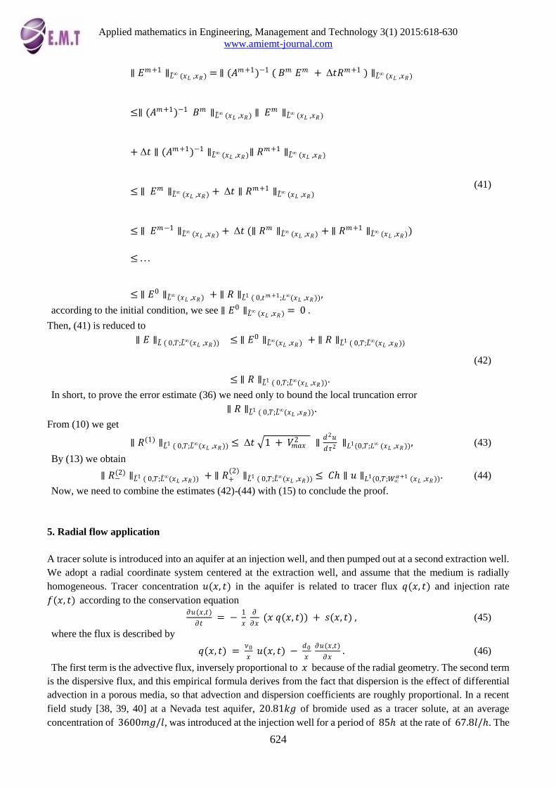
∥ 𝐸𝑚+1 ∥𝐿 ∞ (𝑥𝐿 ,𝑥𝑅) = ∥ (𝐴𝑚+1)−1 ( 𝐵𝑚 𝐸𝑚 + Δ𝑡𝑅𝑚+1 ) ∥𝐿 ∞ (𝑥𝐿 ,𝑥𝑅)
≤∥ (𝐴𝑚+1)−1 𝐵𝑚 ∥𝐿 ∞ (𝑥𝐿 ,𝑥𝑅) ∥ 𝐸𝑚 ∥𝐿 ∞ (𝑥𝐿 ,𝑥𝑅)
+ Δ𝑡 ∥ (𝐴𝑚+1)−1 ∥𝐿 ∞ (𝑥𝐿 ,𝑥𝑅)∥ 𝑅𝑚+1 ∥𝐿 ∞ (𝑥𝐿 ,𝑥𝑅)
≤ ∥ 𝐸𝑚 ∥𝐿 ∞ (𝑥𝐿 ,𝑥𝑅) + Δ𝑡 ∥ 𝑅𝑚+1 ∥𝐿 ∞ (𝑥𝐿 ,𝑥𝑅)
≤ ∥ 𝐸𝑚−1 ∥𝐿 ∞ (𝑥𝐿 ,𝑥𝑅) + Δ𝑡 (∥ 𝑅𝑚 ∥𝐿 ∞ (𝑥𝐿 ,𝑥𝑅) + ∥ 𝑅𝑚+1 ∥𝐿 ∞ (𝑥𝐿 ,𝑥𝑅))
≤ . . .
≤ ∥ 𝐸0 ∥𝐿 ∞ (𝑥𝐿 ,𝑥𝑅) + ∥ 𝑅 ∥𝐿 1 ( 0,𝑡𝑚+1;𝐿∞(𝑥𝐿 ,𝑥𝑅)),
(41)
according to the initial condition, we see ∥ 𝐸0 ∥𝐿 ∞ (𝑥𝐿 ,𝑥𝑅) = 0 .
Then, (41) is reduced to
∥ 𝐸 ∥𝐿 ( 0,𝑇;𝐿 ∞(𝑥𝐿 ,𝑥𝑅)) ≤ ∥ 𝐸0 ∥𝐿 ∞(𝑥𝐿 ,𝑥𝑅) + ∥ 𝑅 ∥𝐿 1 ( 0,𝑇;𝐿 ∞(𝑥𝐿 ,𝑥𝑅))
≤ ∥ 𝑅 ∥𝐿 1 ( 0,𝑇;𝐿 ∞(𝑥𝐿 ,𝑥𝑅)).
(42)
In short, to prove the error estimate (36) we need only to bound the local truncation error
∥ 𝑅 ∥𝐿 1 ( 0,𝑇;𝐿 ∞(𝑥𝐿 ,𝑥𝑅)).
From (10) we get
∥ 𝑅(1) ∥𝐿 1 ( 0,𝑇;𝐿 ∞(𝑥𝐿 ,𝑥𝑅)) ≤ Δ𝑡 1 + 𝑉𝑚𝑎𝑥2 ∥
𝑑2𝑢
𝑑𝜏2 ∥𝐿1(0,𝑇;𝐿∞ (𝑥𝐿 ,𝑥𝑅)), (43)
By (13) we obtain
∥ 𝑅−(2) ∥𝐿 1 ( 0,𝑇;𝐿 ∞(𝑥𝐿 ,𝑥𝑅)) + ∥ 𝑅+
(2)∥𝐿 1 ( 0,𝑇;𝐿 ∞(𝑥𝐿 ,𝑥𝑅)) ≤ 𝐶 ∥ 𝑢 ∥𝐿1(0,𝑇;𝑊∞
𝛼+1 (𝑥𝐿 ,𝑥𝑅)). (44)
Now, we need to combine the estimates (42)-(44) with (15) to conclude the proof.
5. Radial flow application
A tracer solute is introduced into an aquifer at an injection well, and then pumped out at a second extraction well.
We adopt a radial coordinate system centered at the extraction well, and assume that the medium is radially
homogeneous. Tracer concentration 𝑢(𝑥, 𝑡) in the aquifer is related to tracer flux 𝑞(𝑥, 𝑡) and injection rate
𝑓(𝑥, 𝑡) according to the conservation equation
∂𝑢(𝑥 ,𝑡)
∂𝑡 = −
1
𝑥 ∂
∂𝑥 (𝑥 𝑞(𝑥, 𝑡)) + 𝑠(𝑥, 𝑡) , (45)
where the flux is described by
𝑞(𝑥, 𝑡) = 𝜈0
𝑥 𝑢(𝑥, 𝑡) −
𝑑0
𝑥 ∂𝑢(𝑥 ,𝑡)
∂𝑥 . (46)
The first term is the advective flux, inversely proportional to 𝑥 because of the radial geometry. The second term
is the dispersive flux, and this empirical formula derives from the fact that dispersion is the effect of differential
advection in a porous media, so that advection and dispersion coefficients are roughly proportional. In a recent
field study [38, 39, 40] at a Nevada test aquifer, 20.81𝑘𝑔 of bromide used as a tracer solute, at an average
concentration of 3600𝑚𝑔/𝑙, was introduced at the injection well for a period of 85 at the rate of 67.8𝑙/. The
Applied mathematics in Engineering, Management and Technology 3(1) 2015:618-630
www.amiemt-journal.com
625
distance from injection well to the extraction well was 30𝑚, and the radius of extraction well was 0.127𝑚. The
velocity coefficient and the dispersion constant were estimated to be of the same order of magnitude. Measured
concentrations over time at the extraction well show early breakthrough that cannot be explained by the classical
radial flow model. To address this situation, we employ a model with a fractional dispersive flux:
𝑞(𝑥, 𝑡) = 𝜈0
𝑥 𝑢(𝑥, 𝑡) −
𝑑0
𝑥 ∂𝛽𝑢(𝑥 ,𝑡)
∂𝑥𝛽 , (47)
for some 0 < 𝛽 ≤ 1. The fractional term models anomalous dispersion due to velocity contrasts resulting from
the interaction with a porous medium. Note that 𝜈0 and 𝑑0 in Eq.(47) are not the same as in the classical flux
Eq.(46) and the 𝑑0s do not even have the same dimensions. We have emphasized the numerical approximation
method here. See [40] for the details of the tested aquifer and associated parameters. Also, see [25] for a physical
derivation of the fractional flux based on statistical mechanics. The classical model corresponds to a value of
𝛽 = 1. Values of 𝛽 < 1 lead to superdispersion, in which solute spreads faster than the classical model predicts.
See [22, 41] for some practical methods of estimating the order 𝛽 of the fractional derivative from data. In the
limiting case of 𝛽 = 0, the dispersion process is replaced by an advection process in the differential equation.
Substituting (47) with 𝛼 = 𝛽 + 1 into the radial conservation law (45) we get
∂𝑢(𝑥 ,𝑡)
∂𝑡 = −
𝜈0
𝑥 ∂𝑢(𝑥 ,𝑡)
∂𝑥 +
𝑑0
𝑥 ∂𝛼𝑢(𝑥 ,𝑡)
∂𝑥𝛼 𝑠(𝑥, 𝑡) . (48)
Note that Eq.(48) is the same as Eq. (1) with 𝑣( 𝑥) =𝑣0
𝑥 and 𝑑( 𝑟) =
𝑑0
𝑥. We consider this equation and its
numerical solution in the case 1 ≤ 𝛼 ≤ 2, for 𝑥𝐿 < 𝑥 < 𝑥𝑅 and 0 < 𝑡 ≤ 𝑇.
6. Numerical experiments
In this section we carry out numerical experiments to investigate the performance and convergence behavior of
the fractional characteristic finite difference method (CFDM).
6.1. Performance of the fractional characteristic finite difference method for fractional advection -
dispersion flow equations
In this section, We consider following fractional advection - dispersion flow equation:
∂𝑢(𝑥 ,𝑡)
∂𝑡 + 𝑉(𝑥, 𝑡)
∂𝑢(𝑥 ,𝑡)
∂𝑥 − 𝐷 (𝑥, 𝑡)
∂𝛼𝑢(𝑥 ,𝑡)
∂𝑥𝛼 = 𝑠(𝑥, 𝑡) ,
with the coefficients
𝑉(𝑥, 𝑡) = 1 ,𝐷(𝑥, 𝑡) = Γ(3 − 𝑎) 𝑥𝛼 , 𝛼 = 1.8 , 0 ≤ 𝑥 ≤ 2 ,0 < 𝑡 ≤ 1 ,
forcing function
𝑠(𝑥, 𝑡) = −32 𝑒−𝑡 𝑥2 − 2.5 𝑥3 + 25
22 𝑥4 −
1
8(4 𝑥3 − 12 𝑥2 + 8 𝑥) +
1
8𝑥2 (2 − 𝑥)2 ,
the initial condition
𝑢(𝑥, 0) = 4 𝑥2 (2 − 𝑥)2 ,
and the boundary condition
𝑢(0, 𝑡) = ∂𝑢(2,𝑡)
∂𝑡 = 0, 𝑡 ≥ 0.
The exact solution of this fractional advection-dispersion flow equation is given by
𝑢(𝑥, 𝑡) = 4 𝑒−𝑡 𝑥2 (2 − 𝑥)2 .
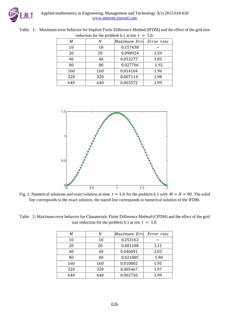
We have shown the exact and numerical solutions in figures 1 and 2. Comparison of Tables 1 and 2 reveals the
reliability of CFDM.
Applied mathematics in Engineering, Management and Technology 3(1) 2015:618-630
www.amiemt-journal.com
626
Table 1: Maximum error behavior for Implisit Finite Difference Method (IFDM) and the effect of the grid size
reduction for the problem 6.1 at tim 𝑡 = 1.0.
𝑀 𝑁 𝑀𝑎𝑥𝑖𝑚𝑢𝑚 𝐸𝑟𝑟𝑜𝑟 𝐸𝑟𝑟𝑜𝑟 𝑟𝑎𝑡𝑒
10 10 0.157438 −
20 20 0.098924 1.59
40 40 0.053277 1.85
80 80 0.027706 1.92
160 160 0.014104 1.96
320 320 0.007114 1.98
640 640 0.003572 1.99
Fig. 1: Numerical solutions and exact solution at time 𝑡 = 1.0 for the problem 6.1 with 𝑀 = 𝑁 = 80. The solid
line corresponds to the exact solution, the stared line corresponds to numerical solution of the IFDM.
Table 2: Maximum error behavior for Charateristic Finite Difference Method (CFDM) and the effect of the grid
size reduction for the problem 6.1 at tim 𝑡 = 1.0.
𝑀 𝑁 𝑀𝑎𝑥𝑖𝑚𝑢𝑚 𝐸𝑟𝑟𝑜𝑟 𝐸𝑟𝑟𝑜𝑟 𝑟𝑎𝑡𝑒
10 10 0.253162 −
20 20 0.081188 3.11
40 40 0.040091 2.02
80 80 0.021085 1.90
160 160 0.010802 1.95
320 320 0.005467 1.97
640 640 0.002750 1.99
Applied mathematics in Engineering, Management and Technology 3(1) 2015:618-630
www.amiemt-journal.com
627
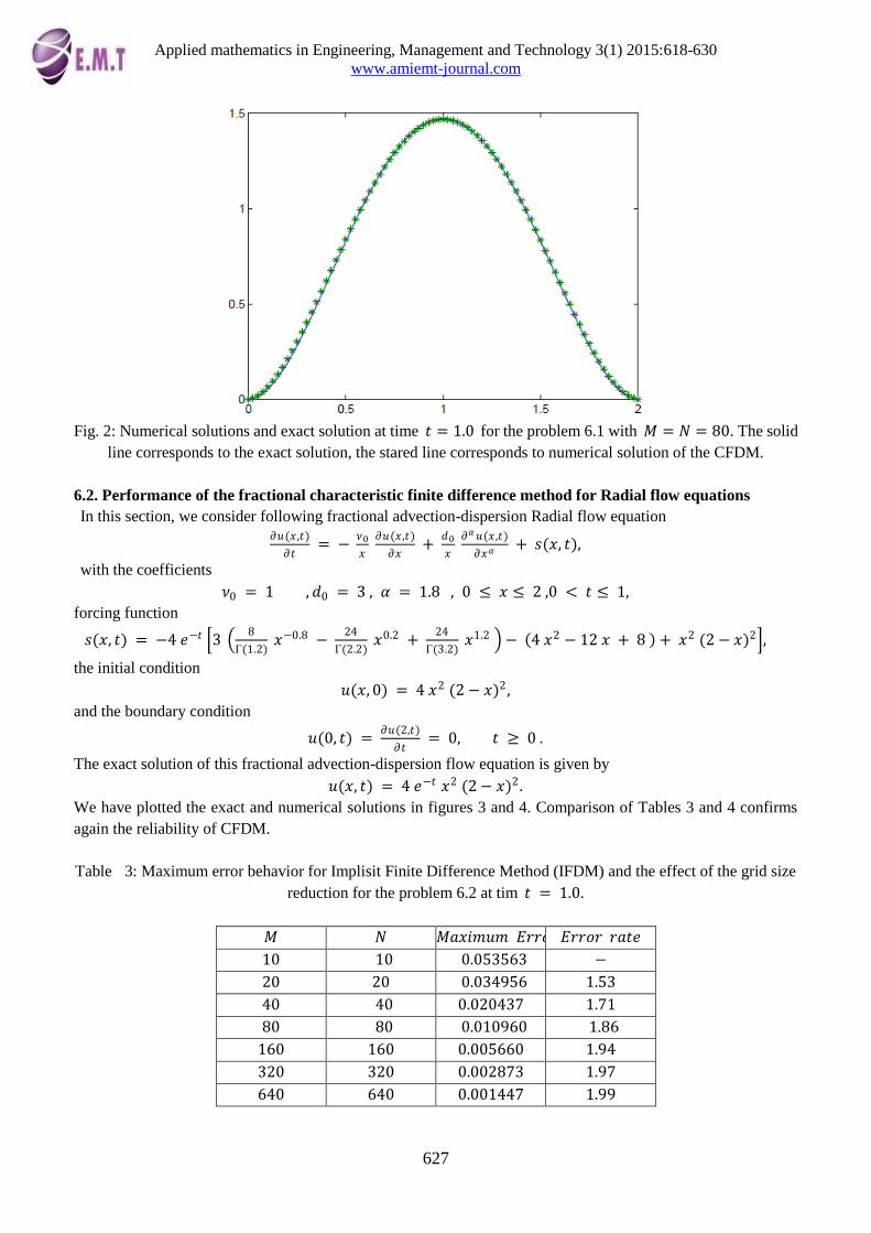
Fig. 2: Numerical solutions and exact solution at time 𝑡 = 1.0 for the problem 6.1 with 𝑀 = 𝑁 = 80. The solid
line corresponds to the exact solution, the stared line corresponds to numerical solution of the CFDM.
6.2. Performance of the fractional characteristic finite difference method for Radial flow equations
In this section, we consider following fractional advection-dispersion Radial flow equation
∂𝑢(𝑥 ,𝑡)
∂𝑡 = −
𝜈0
𝑥 ∂𝑢(𝑥 ,𝑡)
∂𝑥 +
𝑑0
𝑥 ∂𝛼𝑢(𝑥 ,𝑡)
∂𝑥𝛼 + 𝑠(𝑥, 𝑡),
with the coefficients
𝜈0 = 1 , 𝑑0 = 3 , 𝛼 = 1.8 , 0 ≤ 𝑥 ≤ 2 ,0 < 𝑡 ≤ 1,
forcing function
𝑠(𝑥, 𝑡) = −4 𝑒−𝑡 3 8
Γ(1.2) 𝑥−0.8 −
24
Γ(2.2) 𝑥0.2 +
24
Γ(3.2) 𝑥1.2 − 4 𝑥2 − 12 𝑥 + 8 + 𝑥2 (2 − 𝑥)2 ,
the initial condition
𝑢(𝑥, 0) = 4 𝑥2 (2 − 𝑥)2 ,
and the boundary condition
𝑢(0, 𝑡) = ∂𝑢(2,𝑡)
∂𝑡 = 0, 𝑡 ≥ 0 .
The exact solution of this fractional advection-dispersion flow equation is given by
𝑢(𝑥, 𝑡) = 4 𝑒−𝑡 𝑥2 (2 − 𝑥)2 .
We have plotted the exact and numerical solutions in figures 3 and 4. Comparison of Tables 3 and 4 confirms
again the reliability of CFDM.
Table 3: Maximum error behavior for Implisit Finite Difference Method (IFDM) and the effect of the grid size
reduction for the problem 6.2 at tim 𝑡 = 1.0.
𝑀 𝑁 𝑀𝑎𝑥𝑖𝑚𝑢𝑚 𝐸𝑟𝑟𝑜𝑟 𝐸𝑟𝑟𝑜𝑟 𝑟𝑎𝑡𝑒
10 10 0.053563 −
20 20 0.034956 1.53
40 40 0.020437 1.71
80 80 0.010960 1.86
160 160 0.005660 1.94
320 320 0.002873 1.97
640 640 0.001447 1.99
Applied mathematics in Engineering, Management and Technology 3(1) 2015:618-630
www.amiemt-journal.com
628
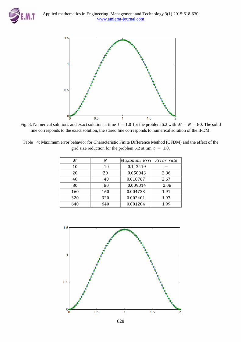
Fig. 3: Numerical solutions and exact solution at time 𝑡 = 1.0 for the problem 6.2 with 𝑀 = 𝑁 = 80. The solid
line corresponds to the exact solution, the stared line corresponds to numerical solution of the IFDM.
Table 4: Maximum error behavior for Characteristic Finite Difference Method (CFDM) and the effect of the
grid size reduction for the problem 6.2 at tim 𝑡 = 1.0.
𝑀 𝑁 𝑀𝑎𝑥𝑖𝑚𝑢𝑚 𝐸𝑟𝑟𝑜𝑟 𝐸𝑟𝑟𝑜𝑟 𝑟𝑎𝑡𝑒
10 10 0.143419 −
20 20 0.050043 2.86
40 40 0.018767 2.67
80 80 0.009014 2.08
160 160 0.004723 1.91
320 320 0.002401 1.97
640 640 0.001204 1.99

Applied mathematics in Engineering, Management and Technology 3(1) 2015:618-630
www.amiemt-journal.com
629
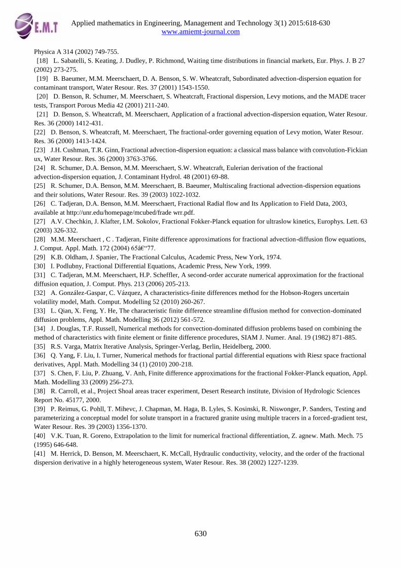
Fig. 4: Numerical solutions and exact solution at time 𝑡 = 1.0 for the problem 6.2 with 𝑀 = 𝑁 = 80. The solid
line corresponds to the exact solution, the stared line corresponds to numerical solution of the CFDM
7. Conclusion
Fractional derivatives in space can be used to model anomalous dispersion/diffusion, where particles spread
faster than the classical models predict. Fractional advection-dispersion equations with variable coefficients
allows velocity to vary over the domain, which is important in applications. An implicit Euler method, based on a
modified Grünwald approximation to the fractional derivative, is consistent and unconditionally stable. If the
usual Grünwald approximation is used, the implicit Euler method is always unstable. This simple numerical
method is useful for solving the fractional radial flow equation, where the fluid velocity increases as flow
converges on an extraction well. The fractional derivative allows the model to more accurately describe early
arrival, which is important in modeling groundwater contamination.
we propose a new finite difference method, called the fractional CFDM, and prove that this new method is
unconditionally stable, consistent and convergent, whose accuracy is of order 𝑂( + Δ𝑡). At the meantime, an
error estimate is given. Numerical experiments are carried out and shown that our new method is much better than
the IFDM. The main advantage of the CFDM is that large time steps can be used without the loss of accuracy,
leading to significantly improved efficiency.
Moreover, the CFDM is especially efficient and superior for the high-dimensional convection-dominated
diffusion equations.
References
[1] K. Miller, B. Ross, An Introduction to the Fractional Calculus and Fractional Differential Equations, Wiley, New York,
1993.
[2] S. Samko, A. Kilbas, O. Marichev, Fractional Integrals and Derivatives: Theory and Applications, Gordon and Breach,
London, 1993.
[3] B. Baeumer, M.M. Meerschaert, Stochastic solutions for fractional Cauchy problems, Frac. Calc. Appl. Anal .4 (2001)
481-500.
[4] E. Barkai, R. Metzler, J. Klafter, From continuous time random walks to the fractional Fokker-Planck equation, Phys.
Rev. E 61 (2000) 132-138.
[5] A. Blumen, G. Zumofen, J. Klafter, Transport aspects in anomalous diffusion: Levy walks, Phys. Rev. A 40 (1989)
3964-3973.
[6] J.P. Bouchaud, A. Georges, Anomalous diffusion in disordered mediastatistical mechanisms, models and physical
applications, Phys. Rep. 195 (1990) 127-293.
[7] A. Chaves, Fractional diffusion equation to describe Levy fights, Phys. Lett. A 239 (1998) 13-16.
[8] J. Klafter, A. Blumen, M.F. Shlesinger, Stochastic pathways to anomalous diffusion, Phys. Rev. A 35 (1987)
3081-3085.
[9] M. Meerschaert, D. Benson, B. Baeumer, Operator Levy motion and multiscaling anomalous diffusion, Phys. Rev. E 63
(2001) 1112-1117.
[10] M. Meerschaert, D. Benson, H.P. ScheXer, B. Baeumer, Stochastic solution of space-time fractional diffusion
equations, Phys. Rev. E 65 (2002) 1103-1106.
[11] M. Meerschaert, D. Benson, H.P. ScheXer, P. Becker-Kern, Governing equations and solutions of anomalous random
walk limits, Phys. Rev. E 66 (2002) 102-105.
[12] M.M. Meerschaert, H.P. ScheXer, Semistable Levy Motion, Frac. Calc. Appl. Anal. 5 (2002) 27-54.
[13] A.I. Saichev, G.M. Zaslavsky, Fractional kinetic equations: solutions and applications, Chaos 7 (1997) 753-764.
[14] E. Scalas, R. Goreno, F. Mainardi, Fractional calculus and continuous-time finance, Phys. A 284 (2000) 376-384.
[15] G. Zaslavsky, Fractional kinetic equation for Hamiltonian chaos. Chaotic advection, tracer dynamics and turbulent
dispersion, Phys. D 76 (1994) 110-122.
[16] R. Goreno, F. Mainardi, E. Scalas, M. Raberto, Fractional calculus and continuous-time finance. III, The diffusion
limit. Mathematical finance (Konstanz, 2000), Trends in Math., Birkhuser, Basel, 2001, pp. 171-180.
[17] M. Raberto, E. Scalas, F. Mainardi, Waiting-times and returns in high-frequency financial data: an empirical study,
Applied mathematics in Engineering, Management and Technology 3(1) 2015:618-630
www.amiemt-journal.com
630
Physica A 314 (2002) 749-755.
[18] L. Sabatelli, S. Keating, J. Dudley, P. Richmond, Waiting time distributions in financial markets, Eur. Phys. J. B 27
(2002) 273-275.
[19] B. Baeumer, M.M. Meerschaert, D. A. Benson, S. W. Wheatcraft, Subordinated advection-dispersion equation for
contaminant transport, Water Resour. Res. 37 (2001) 1543-1550.
[20] D. Benson, R. Schumer, M. Meerschaert, S. Wheatcraft, Fractional dispersion, Levy motions, and the MADE tracer
tests, Transport Porous Media 42 (2001) 211-240.
[21] D. Benson, S. Wheatcraft, M. Meerschaert, Application of a fractional advection-dispersion equation, Water Resour.
Res. 36 (2000) 1412-431.
[22] D. Benson, S. Wheatcraft, M. Meerschaert, The fractional-order governing equation of Levy motion, Water Resour.
Res. 36 (2000) 1413-1424.
[23] J.H. Cushman, T.R. Ginn, Fractional advection-dispersion equation: a classical mass balance with convolution-Fickian
ux, Water Resour. Res. 36 (2000) 3763-3766.
[24] R. Schumer, D.A. Benson, M.M. Meerschaert, S.W. Wheatcraft, Eulerian derivation of the fractional
advection-dispersion equation, J. Contaminant Hydrol. 48 (2001) 69-88.
[25] R. Schumer, D.A. Benson, M.M. Meerschaert, B. Baeumer, Multiscaling fractional advection-dispersion equations
and their solutions, Water Resour. Res. 39 (2003) 1022-1032.
[26] C. Tadjeran, D.A. Benson, M.M. Meerschaert, Fractional Radial flow and Its Application to Field Data, 2003,
available at http://unr.edu/homepage/mcubed/frade wrr.pdf.
[27] A.V. Chechkin, J. Klafter, I.M. Sokolov, Fractional Fokker-Planck equation for ultraslow kinetics, Europhys. Lett. 63
(2003) 326-332.
[28] M.M. Meerschaert , C . Tadjeran, Finite difference approximations for fractional advection-diffusion flow equations,
J. Comput. Appl. Math. 172 (2004)65–77.
[29] K.B. Oldham, J. Spanier, The Fractional Calculus, Academic Press, New York, 1974.
[30] I. Podlubny, Fractional Differential Equations, Academic Press, New York, 1999.
[31] C. Tadjeran, M.M. Meerschaert, H.P. Scheffler, A second-order accurate numerical approximation for the fractional
diffusion equation, J. Comput. Phys. 213 (2006) 205-213.
[32] A. González-Gaspar, C. Vázquez, A characteristics-finite differences method for the Hobson-Rogers uncertain
volatility model, Math. Comput. Modelling 52 (2010) 260-267.
[33] L. Qian, X. Feng, Y. He, The characteristic finite difference streamline diffusion method for convection-dominated
diffusion problems, Appl. Math. Modelling 36 (2012) 561-572.
[34] J. Douglas, T.F. Russell, Numerical methods for convection-dominated diffusion problems based on combining the
method of characteristics with finite element or finite difference procedures, SIAM J. Numer. Anal. 19 (1982) 871-885.
[35] R.S. Varga, Matrix Iterative Analysis, Springer-Verlag, Berlin, Heidelberg, 2000.
[36] Q. Yang, F. Liu, I. Turner, Numerical methods for fractional partial differential equations with Riesz space fractional
derivatives, Appl. Math. Modelling 34 (1) (2010) 200-218.
[37] S. Chen, F. Liu, P. Zhuang, V. Anh, Finite difference approximations for the fractional Fokker-Planck equation, Appl.
Math. Modelling 33 (2009) 256-273.
[38] R. Carroll, et al., Project Shoal areas tracer experiment, Desert Research institute, Division of Hydrologic Sciences
Report No. 45177, 2000.
[39] P. Reimus, G. Pohll, T. Mihevc, J. Chapman, M. Haga, B. Lyles, S. Kosinski, R. Niswonger, P. Sanders, Testing and
parameterizing a conceptual model for solute transport in a fractured granite using multiple tracers in a forced-gradient test,
Water Resour. Res. 39 (2003) 1356-1370.
[40] V.K. Tuan, R. Goreno, Extrapolation to the limit for numerical fractional differentiation, Z. agnew. Math. Mech. 75
(1995) 646-648.
[41] M. Herrick, D. Benson, M. Meerschaert, K. McCall, Hydraulic conductivity, velocity, and the order of the fractional
dispersion derivative in a highly heterogeneous system, Water Resour. Res. 38 (2002) 1227-1239.