chapter_14_radiometric enhancement of landsat imagery

Remote Sensing Analysis

in an

ArcMap Environment

14. Radiometric Enhancement of Landsat Imagery

Tammy E. Parece

James B. Campbell

Remote Sensing Analysis in an ArcMap Environment

Credits

This exercise was developed by:

In partnership with:

Originated by:

James Campbell & John McGee

Tutorials by:

Tammy Parece

Video design and recording by: Laura Johnson

& Eric Guenther

Funded by:

VirginiaView and the AmericaView Consortium

This educational resource (and a broader collection of educational resources) is available for download (.pdf) from the VirginiaView Website. An accompanying video tutorial of this document is

also available through the VirginiaView website: http://www.virginiaview.net/education

For additional information, please contact: John McGee [email protected]

October 2013 Page ii

http://www.virginiaview.net/education

mailto:[email protected]

The instructional materials contained within these documents are copyrighted property of VirginiaView, its partners and other participating AmericaView consortium members. These

materials may be reproduced and used by educators for instructional purposes. No permission is granted to use the materials for paid consulting or instruction where a fee is

collected. Reproduction or translation of any part of this document beyond that permitted in Section 107 or 108 of the 1976 United States Copyright Act without the permission of the

copyright owner(s) is unlawful.

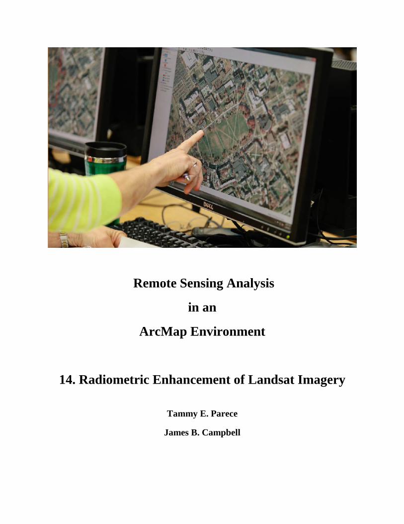
Photo credit for the cover photograph: Christina O’Conner ([email protected]). The authors also acknowledge the support of their academic departments—Virginia Tech Departments of

Geography, and Forest Resources and Environmental Conservation.

October 2013 Page iii

mailto:[email protected]

GIS Tutorial for ArcMap 10.X 14. Radiometric Enhancement of Landsat Imagery

The instructional materials contained within these documents are copyrighted property of VirginiaView, its partners and other participating AmericaView consortium members. These

materials may be reproduced and used by educators for instructional purposes. No permission is granted to use the materials for paid consulting or instruction where a fee is collected.

Reproduction or translation of any part of this document beyond that permitted in Section 107 or 108 of the 1976 United States Copyright Act without the permission of the copyright

owner(s) is unlawful.

In the next few tutorials, you will gain an understanding of the theory of image enhancement using ArcGIS 10.X. This specific tutorial involves radiometric enhancement. Introduction to Image Enhancement

Image enhancement refers to procedures that remote sensing analysts use to adjust the values in a remotely sensed image to improve its visual qualities for a specific purpose. The brightness values at individual pixels are changed to achieve improved brightness, contrast, color balance, or other qualities. The visual quality of an image is related to the range of brightness in the image, known as contrast. A high contrast image has a narrow range of brightness- mainly blacks and whites. A low contrast image has a wide range of brightness. Usually, excessive contrast is undesirable; as the analyst cannot see features depicted in the intermediate grey that usually form the most important part of an image. On the other hand, lack of contrast is usually undesirable as the analyst cannot the edges that form the see the Image enhancement is a tool that permits the analyst to apply the level of contrast appropriate for a specific purpose. It is important to recognize that image enhancement is intended to improve the appearance of a specific image for a specific purpose. Because analysts have different objectives, and images have differing qualities, preferred enhancement techniques will vary from one application to the next. Image enhancement focuses entirely on manipulating the appearance of the image, so it is fundamentally cosmetic in nature, and should not be used as input for analytical purposes. Most remotely sensed images require some form of enhancement because they use only a small range of the brightness available to a computer display, so many of the features depicted on the image are not visible to the analyst. As a result, in its original form, the image may not be suitable for its intended use. Image enhancement applies a strategy for expanding the range of brightness use to display the image, thereby revealing features that might not be visible in the original version.

Enhancing image dynamically in a Viewer is much faster than writing permanent image file for every enhancement operation (and also saves disk space). Therefore, while experimenting to find the desired enhancement, use dynamic (temporary) enhancement in a Viewer. Once you achieve the enhancement that you want, it can be permanently saved.

October 2013 Page 123


Image enhancement can be best discussed in the contact of the frequency histogram of a digital image. A frequency histogram displays image brightness along the horizontal axis, and numbers of pixels at each brightness level along the vertical axis. The shape of a specific histogram is related to the features represented a scene, and conditions under which the image was acquired. Linear Contrast Stretch extends the range of brightness through a systematic expansion of image brightness to occupy the full range of brightness available by creating new intermediate values to generate the necessary range of brightness. Histogram Equalization expands the range of brightness by sliding the brightness along the brightness scale so that they occupy the full range of brightness available in the display. The histogram of the enhanced image shows gaps between the brightness values because they have been separated to create a wider range of brightness in the image. There are a great variety of digital image enhancement techniques. The choice of particular technique(s) depends on the application, data available, experience and preferences of image analyst. In this and the next two tutorials, we will cover the three most important and widely used groups of enhancement techniques:

• Radiometric Enhancement - Enhancing images based on the values of individual pixels (this tutorial)

• Spectral Enhancement - Enhancing images by transforming the values of each pixel on a multiband basis (Band Ratios, Vegetation Indicies, & Tasseled Cap - see Tutorial 15. Spectral Enhancement of Landsat Imagery.)

• Spatial Enhancement - Enhancing images based on the values of individual and neighboring pixels (see Tutorial 16. Spatial Enhancement of Landsat Imagery)

Using ArcGIS as a Viewer for Radiometric Enhancement

Open a map document and load the 7-band composite image that you created in the

tutorial on Creating a Composite Images from Landsat Imagery. Be sure your Image Analysis

window is open. Set your image with band combination 4-3-2. (Note - you can also use these

tools on each of the bands as separate images.)

Left-click on the image name in the Image Analysis window. Once you click on it, it

should activate most of the buttons in the Display window. First, we are going to examine each

one of these buttons and their effects on the viewer. We will then examine histograms (next



section) in two areas, within the Image Analysis/Display window and within the Layer

Properties/Symbology dialog box.

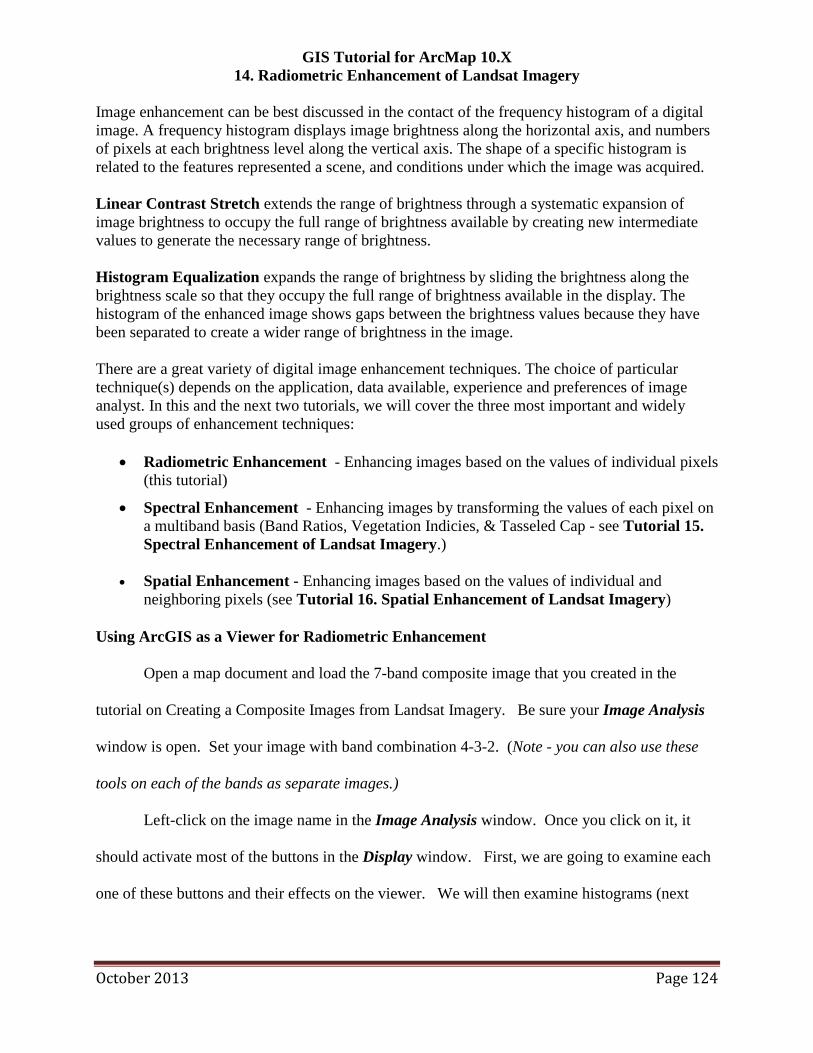
Using the Display window, you can change the Contrast, Brightness, Gamma, and DRA

(dynamic range adjustment) of the image in the map document window by either moving the

sliding bar or placing a numeric value in the box next to the sliding bar. Go ahead and change

the values, one at a time. Observe the changes in your display (note these are only changing the

display, not the original image). Each one changes the display in different ways. Brightness

will make the image appear lighter or darker. Contrast changes the range of differences between

the darkest and lightest objects. Gamma controls relationships between the brightness of

original scene and that on the display. (For example, at a gamma of 1.0, the two images will use

the same scale of brightnesses, whereas at gammas of 0.5 or 1.5, the display shows, respectively,

either compressed, or expanded, scales of brightness relative to the original.) These tools are

useful when doing image classification to help you discern different features within the image.

Contrast Brightness

Transparency Gamma Dynamic Range Adjustment

Background

Zoom to Raster Resolution



We will discuss the list of options within the blue oval in the tutorial on Spatial

Enhancement of Landsat Imagery.

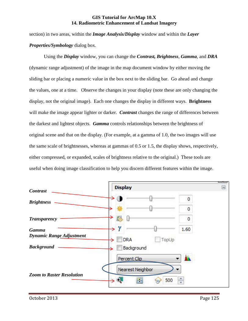
Transparency displays the image so you can see the image below it. If the image below

is an aerial photo, you would be able to see and associate the various brightness values to

specific objects. For example, by adjusting the transparency of the Landsat image (below left)

from 0 (not transparent) to 50 (partially transparent) (below right) you can see that the very

bright area at the top and center corresponds to a building within a parking lot.

(right) Landsat image is opaque, masking view of the aerial photo. (left) Transparency allows a

view of the detail of the aerial photo

To set these values back to the original values, just hit the reset button, which is the icon

for each tool.

By placing a checkmark in the box next to Background you eliminate the no data value

in the display (ArcMap makes Raster files square by adding no value boxes), so you will see the

actual Landsat scene without ArcMap filling it in.



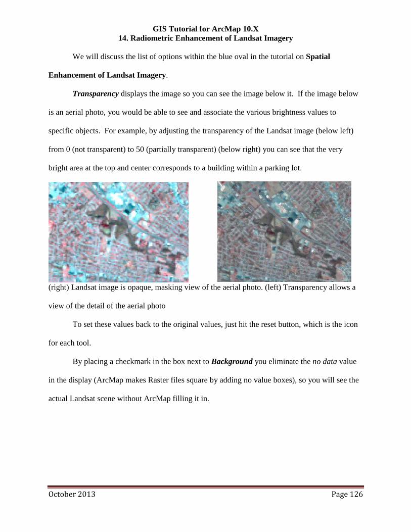
Finally if you hit Zoom to Raster Resolution, the display will zoom in on the image.

Before proceeding to the next steps, please hit the reset button on all the Display buttons,

so we are back to the original images.

Histograms

As stated above, histograms plot the frequency values of the digital numbers (DNs) (x-

axis) against the number of pixels with that value (y-axis). (Remember, the shape of the

histogram is determined by the features represented in the image, and their brightnesses.) We

will discuss histograms in two different areas within ArcMap.

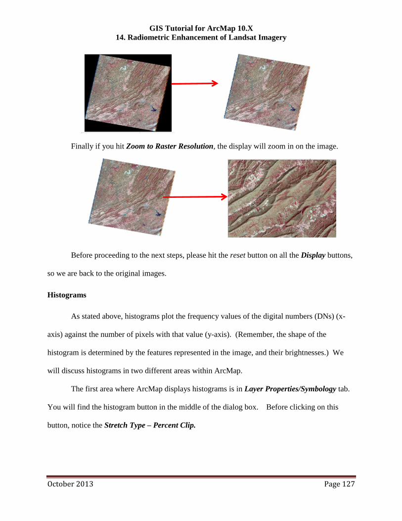
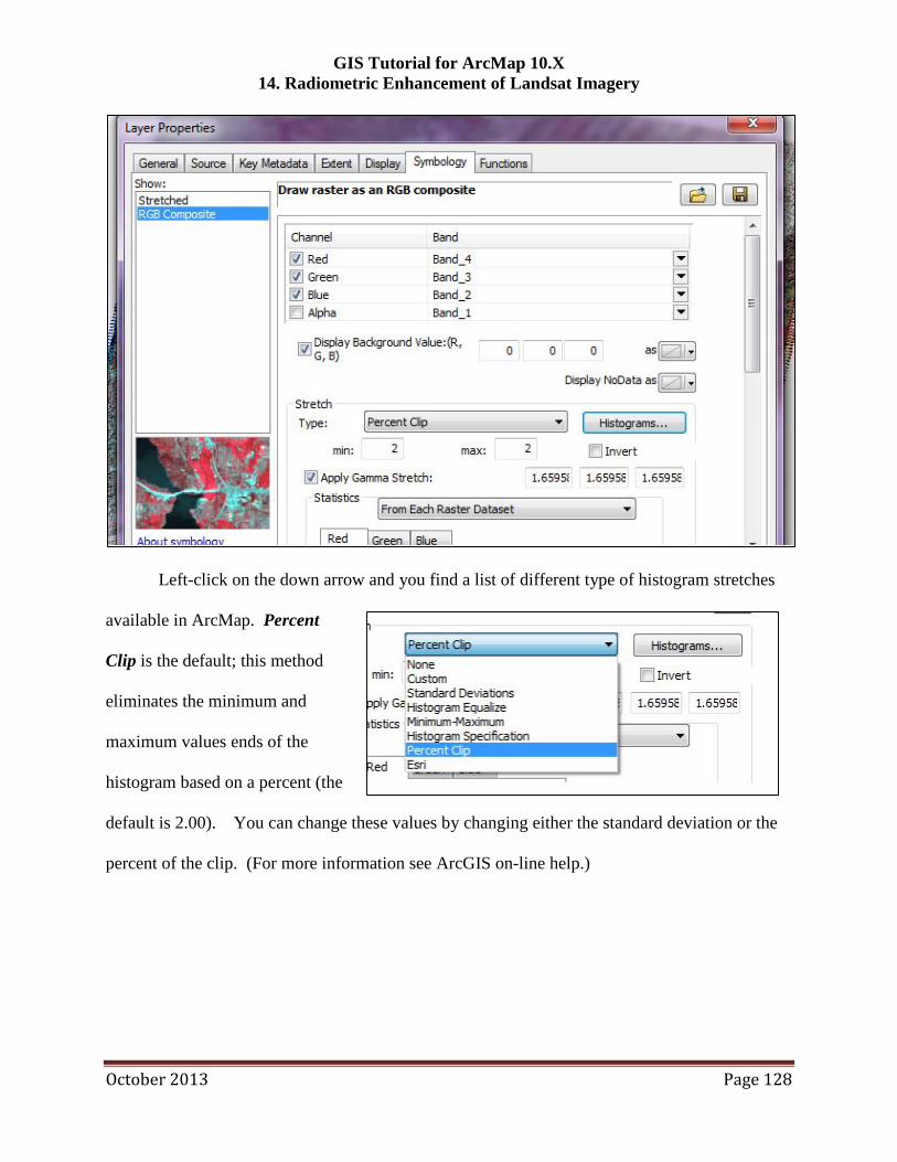
The first area where ArcMap displays histograms is in Layer Properties/Symbology tab.

You will find the histogram button in the middle of the dialog box. Before clicking on this

button, notice the Stretch Type – Percent Clip.



Left-click on the down arrow and you find a list of different type of histogram stretches

available in ArcMap. Percent

Clip is the default; this method

eliminates the minimum and

maximum values ends of the

histogram based on a percent (the

default is 2.00). You can change these values by changing either the standard deviation or the

percent of the clip. (For more information see ArcGIS on-line help.)



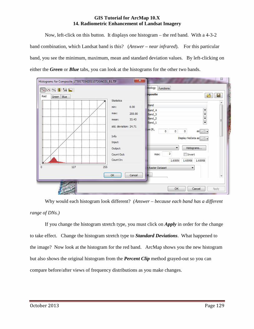
Now, left-click on this button. It displays one histogram – the red band. With a 4-3-2

band combination, which Landsat band is this? (Answer – near infrared). For this particular

band, you see the minimum, maximum, mean and standard deviation values. By left-clicking on

either the Green or Blue tabs, you can look at the histograms for the other two bands.

Why would each histogram look different? (Answer – because each band has a different

range of DNs.)

If you change the histogram stretch type, you must click on Apply in order for the change

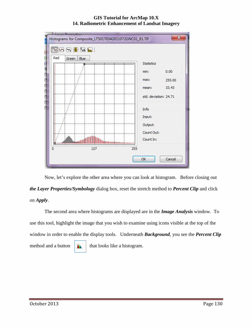
to take effect. Change the histogram stretch type to Standard Deviations. What happened to

the image? Now look at the histogram for the red band. ArcMap shows you the new histogram

but also shows the original histogram from the Percent Clip method grayed-out so you can

compare before/after views of frequency distributions as you make changes.



Now, let’s explore the other area where you can look at histogram. Before closing out

the Layer Properties/Symbology dialog box, reset the stretch method to Percent Clip and click

on Apply.

The second area where histograms are displayed are in the Image Analysis window. To

use this tool, highlight the image that you wish to examine using icons visible at the top of the

window in order to enable the display tools. Underneath Background, you see the Percent Clip

method and a button that looks like a histogram.



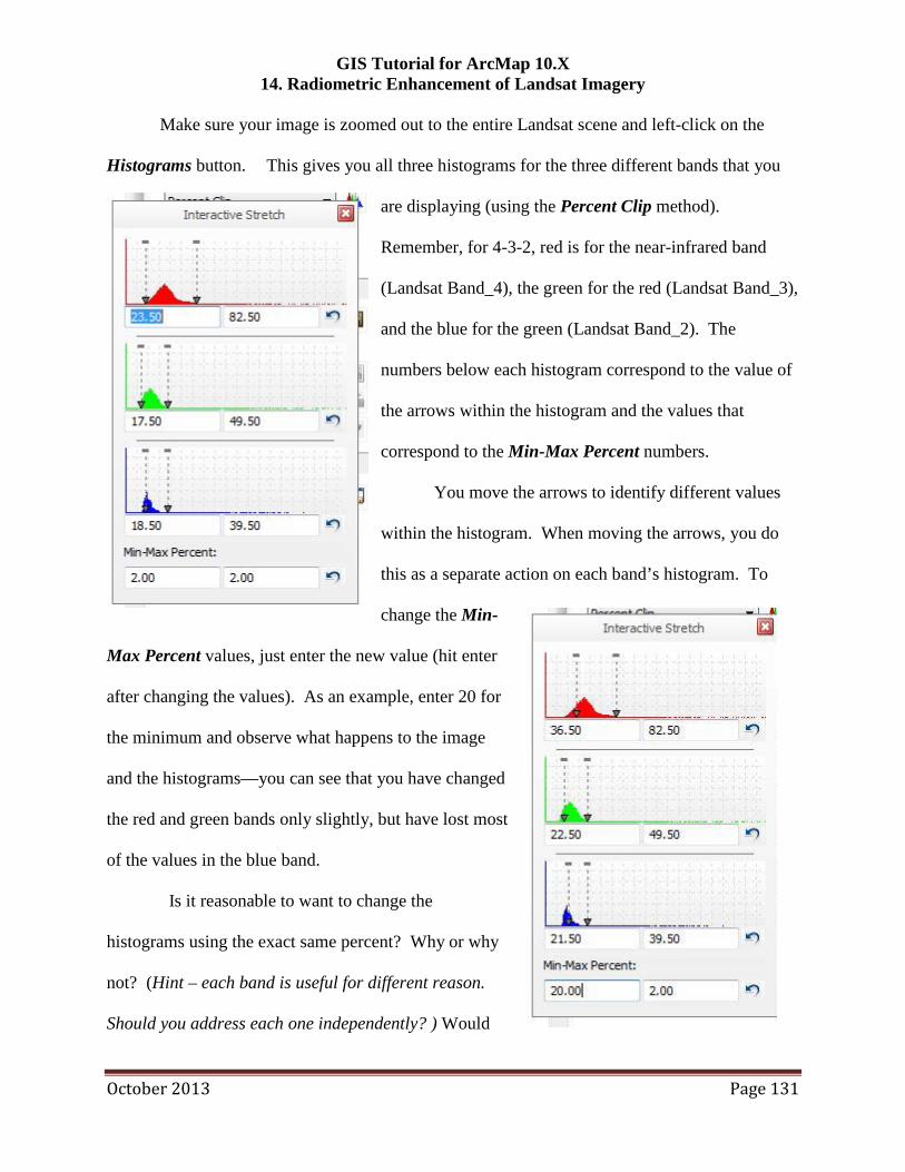
Make sure your image is zoomed out to the entire Landsat scene and left-click on the

Histograms button. This gives you all three histograms for the three different bands that you

are displaying (using the Percent Clip method).

Remember, for 4-3-2, red is for the near-infrared band

(Landsat Band_4), the green for the red (Landsat Band_3),

and the blue for the green (Landsat Band_2). The

numbers below each histogram correspond to the value of

the arrows within the histogram and the values that

correspond to the Min-Max Percent numbers.

You move the arrows to identify different values

within the histogram. When moving the arrows, you do

this as a separate action on each band’s histogram. To

change the Min-

Max Percent values, just enter the new value (hit enter

after changing the values). As an example, enter 20 for

the minimum and observe what happens to the image

and the histograms—you can see that you have changed

the red and green bands only slightly, but have lost most

of the values in the blue band.

Is it reasonable to want to change the

histograms using the exact same percent? Why or why

not? (Hint – each band is useful for different reason.

Should you address each one independently? ) Would



you use the same method to assist in feature identification -- forest areas versus the city? Why or

why not?

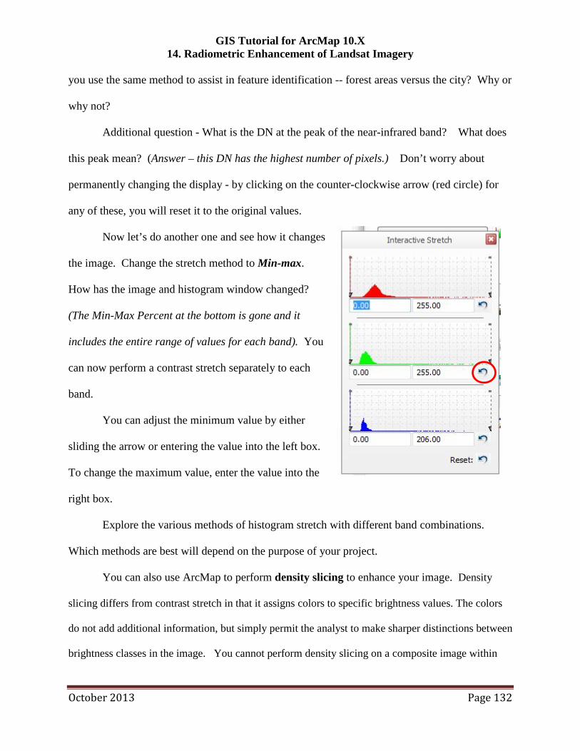
Additional question - What is the DN at the peak of the near-infrared band? What does

this peak mean? (Answer – this DN has the highest number of pixels.) Don’t worry about

permanently changing the display - by clicking on the counter-clockwise arrow (red circle) for

any of these, you will reset it to the original values.

Now let’s do another one and see how it changes

the image. Change the stretch method to Min-max.

How has the image and histogram window changed?

(The Min-Max Percent at the bottom is gone and it

includes the entire range of values for each band). You

can now perform a contrast stretch separately to each

band.

You can adjust the minimum value by either

sliding the arrow or entering the value into the left box.

To change the maximum value, enter the value into the

right box.

Explore the various methods of histogram stretch with different band combinations.

Which methods are best will depend on the purpose of your project.

You can also use ArcMap to perform density slicing to enhance your image. Density

slicing differs from contrast stretch in that it assigns colors to specific brightness values. The colors

do not add additional information, but simply permit the analyst to make sharper distinctions between

brightness classes in the image. You cannot perform density slicing on a composite image within

October 2013 2


ArcMap,--density slicing can only be accomplished on each individual band image that you received

with your Landsat download. This procedure is beyond the scope of this tutorial.

We will discuss further Image Enhancement techniques in the next two tutorials on

Spectral Enhancement of Landsat Imagery and Spatial Enhancement of Landsat Imagery.

As a review: Spectral Enhancement transforms the values of each pixel on a multiband

basis (Band Ratios, Vegetation Indices, & Tasseled Cap) and Spatial Enhancement enhances

images based on the values of individual and neighboring pixels


chapter_14_radiometric enhancement of landsat imagery

Documents