chapter1 march b28
TRANSCRIPT

Monitoring of
Energy Efficiency Upgrades
in State Houses in
southern New Zealand
Monitoring of
Energy Efficiency Upgrades
in State Houses in
southern New Zealand
Bob Lloyd
Maria Callau
Funded by FRST - Grant # UOOX0206
A research project by the Energy Management Group
Physics Department - University of Otago
Heat Transfer
Air Inf
iltrati
onHEAT
Thermal Properties
of Materials

March 2006
A research project by the Energy Management Group Physics Department - University of Otago
Dunedin – New Zealand

Executive Summary
A
Executive Summary
Synopsis
The status of a nation’s housing stock in terms of comfort and energy efficiency is an indicator of some importance. There is considerable evidence to suggest that cold damp houses impose health risks on the occupants that are unacceptable in developed countries. In addition, in an energy constrained world, the energy costs of fulfilling the comfort requirements suggests that the thermal efficiency of the housing stock be optimized. Historically the housing stock in NZ has not fulfilled either criterion, that is, they are neither warm nor energy efficient by OECD standards. Predictably, housing at the lower end of the market, including public housing, exhibits some of the worst excesses in this regard. It is to the credit of the NZ Government that they have embarked on a program to improve the situation by having Housing NZ implement a national energy efficiency upgrade program for public housing.
Unfortunately our research suggests that the current implementation of this upgrade program has not produced significant improvement in either thermal comfort or energy efficiency, at least in the colder regions of the country.
These findings were quite surprising in the first instance. The upgrade program had the goal of making houses warmer by reducing heat loss through improved thermal insulation in the houses. Our results showed a small improvement but overall the indoor temperatures observed in the southern regions of the South Island did not come close to those recommended for healthy living. The reasons for the small improvement were multiple and included factors such as the public houses being originally poorly built from a thermal viewpoint; with heat losses through the un-insulated light frame walls, leaky windows, single glass panes and large gaps in the external building fabric (especially in the
suspended floors) still remaining significant after the upgrade.
The R value of the macerated paper insulation applied to the ceiling cavity was not known and it was thought that extra insulation would be needed to bring the ceiling up to the level proposed by EECA. Finally, and importantly, the occupants were (and still are) accustomed to providing little heating to living areas and even less to bedrooms. Adequate indoor temperatures cannot be reached in a cool climate if there is little or no space heating, unless there is significant internal and (or) solar gain. Let’s be clear what we are not saying, we are not saying that insulating building fabric in residential housing is a bad idea. Insulation is almost always a cost effective method of reducing heat losses in building structures. In the present case, however, the level of insulation extended to only a portion of the building fabric of which the most important section, the ceiling, had already been previously upgraded; and the occupants used a low level of space heating. Circumstances which when put together have meant that the efficacy of the upgrade has been limited. Our conclusions from the study suggest that upgrades for residential housing in NZ need to move on from the basic ceiling/floor upgrades to include insulation of the whole building fabric to levels at least consistent with existing building standards in NZ. The Study
The study area was located in the far south of the South Island of New Zealand. It included the three cities: Dunedin, Gore and Invercargill. Public housing in this area was originally built during the 1940s and 50s to provide budget accommodation for low income households. Public housing in this area can be grouped into three general categories: 1940-50’s weatherboard, 1940-50’s brick veneer, and the late 1970’s (and later) masonry veneer houses. The main structural and material differences between these categories are significant in terms of thermal comfort.
Executive Summary
B
The Housing New Zealand Corporation (HNZC) had 64,400 state and community properties nationwide as of June 2003 (HNZC, 2003). HNZC has been investing about four million NZ dollars annually to upgrade all of its pre-1978 housing stock with regards to energy efficiency since 2001. Houses in the colder climate regions have been given priority in the first years of the program. These houses were originally built with no insulation. However, a previous retrofit in the 70s’ had provided some insulation above the ceiling.
Upgrades to the houses in the current program included ceiling insulation (polyester fibre blankets added above an existing insulation) and sub floor insulation (perforated aluminium foil). Also a small number of hot water cylinders were insulated and brush type draught stoppers were installed to the house main entrance doors to prevent cold air entering the house from the gaps.
The research, funded by the Foundation for Science Research and Technology (FRST) and undertaken by Otago University, monitored the upgrade program from the second year (Dec 2002) for the southern region of NZ. From the 490 houses participating in the program in that year, a sample selection of 111 houses was made. Houses were divided into three samples. Sample A and B in Dunedin and C in Invercargill and Gore. Samples A and C were upgraded first and Sample B was upgraded the following year allowing a before and after comparison to be made. The main field monitoring was completed by the end of 2004 after which modelling and intensive investigation of a few houses took place.
Equipment was installed in order to monitor the houses and thus to identify improvements after the upgrade. The monitoring recorded changes in indoor temperatures and energy input as well as ambient weather conditions.
A household survey, using questionnaires, was undertaken at the outset of the project in order to collect data on household energy use, comfort conditions, and socio/demographic characteristics. Information about the building structure, house plan and other aspects pertinent to
each house was also collected so that thermal modelling could be completed.
Temperatures
By comparing the surveyed houses in 2003 with 2004 and taking into consideration changes in weather conditions, the results showed that after houses were upgraded only a small improvement was recorded in indoor temperatures. The bottom line was an increase of 0.4°C in average annual temperatures after upgrading. The increase for winter months (June to August) was 0.6°C for living areas and bedrooms. Improved insulation was able to increase net temperature differences (the difference between the indoor and the outdoor temperatures) after space heating was applied in the living areas. However, generally low levels of space heating meant that increases in absolute temperatures in the houses were minimal. Unfortunately the gain in living room temperatures was most pronounced in the late evening, probably after the rooms were unoccupied for the night.
Occupants were found to be exposed to absolute indoor temperatures considerably below the WHO recommended minimum of 16°C. Houses in Dunedin recorded average indoor temperatures of 14.9°C in living areas and 13.4°C in bedrooms averaged over the years 2003 and 2004. Alarmingly occupants could be exposed to indoor temperatures of less than 12°C, for nearly half (48%) of a 24 hour day during the three winter months of June, July and August. Also, the minimum temperature (averaged over the sample) recorded in those months was between 5°C and 5.4°C with little improvement after the upgrade.
The measured data showed about a 6% reduction in relative humidity in the living rooms after the insulation upgrade. This reduction at 10-15°C would come from a 0.4°C increase in temperature and thus is consistent with the measured 0.4°C annual average improvement in indoor temperature.
Energy Usage
The annual mean household total energy use for all Dunedin houses in the study was 8690 kWh, with 78% being for electricity and 22% for other fuels.
Executive Summary
C
After correction of the space heating energy use for weather conditions, a reduction of between 7% and 13% in electricity consumption was recorded after the upgrade for Dunedin houses participating in the research. This reduction represents between 5% and 9% of the total household energy use. The weather corrected decrease in “other fuels” was -16% (ie. an increase) for Sample A and +34% for Sample B comparing 2003 with 2004 but with a standard deviation in the mean consumption of “other fuels” of 22% neither change could be considered significant.
Energy consumption for water heating was found to account for around 35% of the total year electricity consumption for the study houses. This percentage is in good agreement with other studies (Isaac N., et al. 2005). There was about an 18% net increase in electricity consumption for water heating in winter. There was no significant reduction of hot water energy consumption after the upgrade. This was due to the fact that only 2% of the cylinders having been insulated during the upgrade program because of the lack of space around the cylinders to place the wrap. The measured hot water energy consumption for the survey sample was some 19% lower than the national average found by BRANZ in their HEEP study (EECA 2001).
Modelling
As the efficacy of the HNZC upgrade program was not obvious from the main monitoring program, two State houses participating in the energy efficient upgrade program located in Dunedin were selected to be intensively monitored over a short time period. The aim was to identify specific improvements in the thermal performance of the building envelope after both houses were upgraded. Results were compared with computer modelling
Results from these houses showed a measured increase in the thermal resistance (R value) of the building envelope of 8% compared to an increase of 12% obtained using a steady state resistance model.
Modelling the HNZC Dunedin houses before and after the upgrade package was
undertaken using ALF3 (NZ) and Virtual Environment (UK). Houses were modelled using a typical heating schedule similar to that reported by the householders participating in the program. An increase of around 0.5°C in annual average indoor living room temperature was predicted by both packages assuming a constant use of space heating. This result was consistent with our measurements which showed an increase of 0.4°C + 0.2°C in living room temperatures but with a concurrent reduction of between 1/5 and 1/3 of electricity usage for space heating. Virtual Environment simulation gave 20% reduction in space heating energy per annum for no increase in indoor temperature. This would amount to a reduction of 6% in total household energy consumption.
In addition the modelling showed that a typical state house in Dunedin would need between 12,800kWh and 15,400kWh for space heating to maintain a constant indoor temperature of even 16ºC (the lower value being for the house after the upgrade and the higher value for the house before the upgrade). The energy needed increased by around 25% when the indoor temperature was increased to 18ºC. This energy requirement is considerably higher than the measured energy consumption from the households participating in the program. The measurements suggested that less than 3,000 kWh on average per household was used for space heating (see chapter 5); a factor of 5 lower than that needed even for a basic temperature of 16ºC. The HNZC houses in Dunedin were drastically under-heated by developed world standards.
A typical State house was analyzed by using standard component thermal resistances for each material in the building fabric in order to understand the heat flow through the building envelope. Three physical progressions of upgrading were identified and analyzed (original, 70’s retrofit and current upgrade). The figure below shows heat losses through the different components for each of these three stages.

Executive Summary
D
0
20
40
60
80
100
120
140
160
180
200
Ceiling External Wall Windows Floor Air infiltration
W/˚
Cnon insulated (original) 70s upgrade 2004 upgrade
Comparison of heat losses through the different components of the building envelope for a typical State House: original vs. ’70s retrofit vs. 2004 upgrade package.
As can be seen there was a considerable reduction of heat loss through the ceiling after the first upgrade. After this upgrade around 90% of heat losses occurred through building components other than the ceiling. The current energy efficiency upgrade package targeted insulation of the ceiling and sub floor. As might be expected, insulating the ceiling only offered a small improvement over the earlier upgrade, reducing the loss through the ceiling to 5% from the earlier 10%. While this improvement was 50% in terms of the loss through the ceiling only, the overall improvement after the upgrade was only a 5% reduction. Improving the floor had an impact in further reducing 8% of the overall heat losses. Un-insulated walls and single glazed wooden frame windows accounted for more than 60% of the losses, while air infiltration represented some 19%. In terms of the total heat losses, there was a possible reduction of 23% after the first ‘70s retrofit but only a further 15% after the latest upgrade.
Conclusions
The final result was a small increase of around 0.4ºC in annual indoor temperatures (0.6ºC in winter months) and a decrease in electrical energy consumption of around between 5% and 9% after a relatively modest upgrade package. It is important to note that there has been no real improvement in absolute indoor temperatures since at least 1972.
Improving insulation, at the levels applied (ceiling insulation and limited under floor insulation), has not significantly improved indoor temperatures in the southern part of the South Island in NZ to levels that would be considered healthy.
These results together with the thermal modelling suggest that if no indoor temperature increase was achieved after the upgrade, then a reduction of between 6% and 10% in total energy consumption for Dunedin houses participating in the research might be expected. An energy saving for a 10% reduction in total electricity use is equivalent to around 870kWh per year, which would cost $NZ156 (at $0.18/kWh) and save 160 kg of CO2 (using the 2004 figures for electricity generation and CO2 emissions in NZ of 0.185 kg CO2 per kWh). The savings would equate to a simple pay back time of 10 years as the initial cost of the upgrade package was around $1,600 (2004 prices).
The above analysis indicates that household energy savings in electricity use after the insulation upgrade would be at best marginal. The reasons for this small improvement in both temperature increase and energy reduction was due primarily to two factors, the marginal improvement in insulation afforded by the new ceiling insulation over the existing “insulfluf” and the low rate of heating of the homes. The second factor introduces a major risk in terms of the upgrade contributing to increased thermal comfort; that is, if the householders do not heat the houses then adequate thermal comfort will not be obtained.
It is clear that the simple insulation upgrade that involved only one aspect of the building fabric was not a complete solution due to the poorly built and not well heated public HNZC housing. If improving indoor thermal comfort and at the same time making energy efficiency at homes were the goal, then more intensive housing insulation measures or better home energy efficiency technologies would need to be applied.
These findings were quite surprising in the first instance. The upgrade program had the goal of making houses warmer by reducing heat loss through improved thermal insulation in the houses. Our results showed a small improvement but overall the indoor temperatures observed in the southern regions of the South Island did not come close to those recommended for healthy living. The reasons for the small improvement were multiple and involved factors such as the public houses being

Executive Summary
E
originally poorly built from a thermal viewpoint, with heat losses through the un-insulated light frame walls, leaky windows, single glass panes and large gaps in the external building fabric (especially in the suspended floors) still remaining significant after the upgrade.
The R value of the macerated paper insulation applied to the ceiling cavity was not known and it was thought that extra insulation would be needed to bring the ceiling up to the level proposed by EECA. Temperature differences between the older and the newer homes were the most significant in the study and are a clear indication of the thermal improvement presented in the later vintage houses. Houses with enclosed solid fuel heaters presented significantly higher indoor temperatures than those without. Houses with unsealed open fires presented significantly lower indoor temperatures than those without.
Finally, and importantly, the occupants were (and still are) accustomed to providing little heating to living areas and even less to bedrooms. Adequate indoor temperatures cannot be reached in a cool climate if there is little or no space heating, unless there is significant internal and (or) solar gain.
Further work
Further work will need to be completed in order to firm up on any recommendations that may lead to solutions of some of the questions posed by the study. In particular, we intend to progress the computer modelling to look at alternative scenarios for improved upgrades. In addition we intend to complete further field work looking at installing double glazing and high efficiency light bulbs. We are also planning the complete refurbishment of up to two HNZC houses up to the present (1996) building standards to quantify the improved thermal environment and to detail the costs of completing the upgrade. Further investigations will also take into account possible mass transfer of water vapour within the wall cavity.
Interim Recommendations
Quantify air leakage and improvements before and after the upgrades. Achieve a minimum of 0.75 ACH.
Replace old inefficient hot water cylinders for new efficient ones. Investigate ways of introducing a subsidized solar heating package (including heat pump hot water systems) into public rental housing. Adjusting the thermostat for hot water cylinders should be a mandatory component of any upgrade process.
Encourage efficient space heating in HNZC homes and exploring options for installation of subsidized equipment, such as space heating heat pumps and energy efficient wood burners if necessary.
It is thought to be a high priority that all existing open fires be sealed and replaced with energy efficient appliances.
Consideration should be given to providing curtains with pelmets instead of applying ceiling insulation to houses for the remainder of the upgrade program. It is also likely that under floor insulation with fiberglass batts will be of greater benefit than the under floor foil insulation but this will be confirmed in the next set of studies to be undertaken.


Index
i
Index
Executive Summary A-E Index i Figures iii Graphics v Abbreviations vi Acknowledgements vi Chapter One – Introduction
1.1 Research 1 1.2 Climate, Energy Use and Thermal Comfort in New Zealand Homes New Zealand Climate New Zealand Building Regulations Findings on Indoor Temperatures from Previous Studies
1 1 2 2
1.3 The Study Area 4 1.4 Public Housing and the HNZC Energy Efficiency Upgrade Program Public Housing The Energy Efficiency Upgrade Program Energy Efficiency Upgrade Package implemented in the houses participating
in the research
5 5 5 6
Chapter Two – Sample Selection & Data Collection Methodology
2.1 Sample Selection 7 2.2 Physical Measurements and Data Collection Methodology
Physical Data Energy Equipment Installed for monitoring
8 8 8 8
Chapter Three – Results: Socio-Economic Survey
3.1 Results The occupants: Age & Income Energy consumption and space heating sources Hot Water Physical Characteristics of houses Similarities and Differences between the Sample Occupant Perceptions
10 10 11 11 13 13 14
3.2 Discussion on the possible Biases in the Survey 14
Chapter Four – Results: Temperature and Relative Humidity
4.1 Ambient Weather Conditions 15 4.2 Indoor temperature in the monitored houses Exposure to indoor temperatures
Indoor temperature variations due to differences in house structure and vintage
16 19 20
4.3 First Comparison of the Measured indoor temperatures
between Sample A(upgraded) and Sample B (non upgraded) in 2003 21
4.4 Second Comparison of the Measured indoor temperatures for the same Sample of houses before and after the upgrade Sample A (2003-2004) Sample B (2003-2004) Summary
24
24 24 25
4.5 24 Hour Indoor temperatures profiles 25 4.6 Relative Humidity Results 27

Index
ii
Chapter Five – Results: Energy Use in the Study Houses
5.1 Household Electricity Usage
Measured Household Electricity Consumption in the detailed monitored houses
Household Electricity Consumption for all the Sample houses
30 30
31
5.2 Electricity Usage for Water Heating 33 5.3 Continuous Load and Standby Power losses 35 5.4 Energy use for Solid Fuels and LPG 36 5.5 Total Energy Use for houses in Sample A & B 36 5.6 Comparison of Energy Use for the same Sample of houses in 2003 and 2004
(with different weather conditions and same occupants) Sample A Sample B Summary
39
39 40 41
Chapter Six – Intensive monitoring of two state houses in Dunedin
6.1 Methodology
Steady State Analysis Monitoring Process Modelling
42 42 42 43
6.2 The two Houses 43 6.3 Results: Modelling the theory 45 6.4 Results: Physical monitoring of the houses House 1 House 2 Summary
46 46 46 47
6.5 Results: Modelling with Virtual Environment 48 6.6 Computer Modelling vs. Real Data: Sample A & B in Dunedin Modelling with Virtual Environment Modelling with ALF3 Comparing modelling with measurements…
51 51 51 52
Chapter Seven – Summary of Results
7.1 Indoor Temperature and Relative Humidity 54 7.2 Energy Usage 55 7.3 Indoor Air Quality 56 7.4 Modelling and single house investigation 56 7.5 Computer Modelling Results 57 7.6 Perception of the Occupants 58
Chapter Eight – Conclusions and Recommendations
8.1 Conclusions 59 8.2 Further work / Recommendation 62
References 64 Appendix A – Blower Door Report I Appendix B – Energy Efficiency Household Survey – Part A III Appendix C – Energy Efficiency Household Survey – Part B V

Index
iii
Figures Chapter One
Figure 1.1 Typical Public Houses in the Southern Region
Chapter Three – Results: Socio-Economic Survey
Figure 3.1 Age of the Surveyed houses in Dunedin and Southland Figure 3.2 Ranking of Energy Sources as the First Choice for Space Heating Figure 3.3 Energy Grades of Surveyed Hot Water Heaters Figure 3.4 Power Ratings of the Hot Water Cylinders Heating Element for samples in
Dunedin Figure 3.5 Measured Hot Water temperatures for the surveyed houses Figure 3.6 Shower flow rate and daily shower usage for all the surveyed houses Figure 3.7 Perception of Comfort of the Surveyed Householders before the upgrade
Chapter Four – Results: Temperature and Relative Humidity
Figure 4.1 Weather Data for the Years of 2002, 2003, 2004 and the past 30 Year Average Figure 4.2 Temperature Variation for all monitored houses Sample A, B & C for Livingrooms
and Bedrooms (2003 – 2004) Figure 4.3 Histograms of houses in Sample A & B showing percentage of data recorded
below 12°C and below 18°C in winter time – Livingrooms and Bedrooms Figure 4.4 Histograms of Samples A & B showing % of houses that recorded improvement
of NTD after upgrade in winter months – Livingrooms & Bedrooms Figure 4.5 Histograms of absolute minimum temperatures for bedrooms during “sleep-
hours” and living areas during “awake-hours” in Sample B houses during winter months (2003 vs. 2004)
Figure 4.6 Indoor Temperatures in different types of houses in Dunedin (Dec 2002 – July 2004) 1970’s, Brick (’50) and Weatherboard (’50). Sample A & B
Figure 4.7 Monthly Mean Temperatures Upgraded vs. Non-upgraded Houses in Living Rooms and Bedrooms (2003 – 2004)
Figure 4.8 Comparison of Daily Mean Temperatures in Living Rooms and Bedrooms between upgraded and Non-upgraded Houses in Dunedin in winter 2003
Figure 4.9 24 Hours Temperature Profiles for houses in Sample A - January 2003 & 2004 Figure 4.10 24 Hours Temperature Profiles for houses in Sample A & B - June 2003 & 2004 Figure 4.11 Monthly Mean Relative Humidity for D1-D22 Houses from December 2002 to July
2004 Figure 4.12 The 24 Hours Mean Relative Humidity Changes for Di-D22 Houses in January and
July 2003 Figure 4.13 Comparison of Mean % of hourly Relative Humidity data exceeded 70% RH
between the Ambient Air and the Indoor Air (before and after the upgrade) for D1-D22 Houses
Chapter Five – Results: Energy Use in the Study Houses
Figure 5.1 Monthly Electricity Consumption for the 30 detailed monitored houses in Dunedin, Invercargill and Gore from December 2002 to July 2004
Figure 5.2 The 24 Hour Monthly Mean Household Electricity Load Patterns for D1-D22 Houses in Dunedin in 2003
Figure 5.3 The 24 Hour Monthly Mean Space Heating Patterns for D1-D22 Houses in Dunedin from January to July 2003
Figure 5.4 Monthly Mean Electricity Consumption for the 111 Monitored Houses (2003-2004) Figure 5.5 Electricity Consumption for Sample A – Whole Year & Winter (July-Aug) Historical
Household Electricity Consumption (before upgrade) vs. Measured Household Electricity Consumption (after upgrade)
Figure 5.6 Electricity Consumption for Sample C – Whole Year & Winter (July-Aug) Historical Household Electricity Consumption (before upgrade) vs. Measured Household Electricity Consumption (after upgrade)
Figure 5.7 Measured Household Electricity Consumption for Sample B – Whole Year & Winter (June-Aug) before vs. after upgrade

Index
iv
Figure 5.8 Histogram of the Monthly Mean Electricity Consumption for Water Heating for the 111 monitored houses from December 2002 to July 2004
Figure 5.9 Monthly Electricity Consumption for hot water & non hot water for the monitored period for each Sample
Figure 5.10 Percentages of Mean Monthly Electricity Consumption for Water Heating against the Monthly Household Total Electricity Usage
Figure 5.11 Total Energy and electricity consumption for houses in Sample A & B in Dunedin in 2003 and 2004
Figure 5.12 Comparison of the Monthly Mean Household Energy Use between houses in Sample A and Sample B in Dunedin in 2003
Figure 5.13 Comparison of the Monthly Mean Household Energy Use and hot water for houses in Sample A in 2003 & 2004
Figure 5.14 Comparison of the Monthly Mean Household Energy Use and hot water for houses in Sample B in 2003 & 2004
Chapter Six – Intensive Monitoring of Two State Houses in Dunedin
Figure 6.1 Aerial photo on both houses (18 Dover St. & 22 Forrester St. Pine Hill, Dunedin) Figure 6.2 Houses layout. House 1 & House 2 Figure 6.3 House 1: % of heat losses through the different components of the building
envelope Figure 6.4 House 2: % of heat losses through the different components of the building
envelope Figure 6.5 Comparison of heat losses through the different components of the building
envelope: original vs. ‘70s retrofit vs. 2004 upgrade package (House 1 & 2) Figure 6.6 House 1: Thermal performance of Bedroom 2 – VE vs. measured before and
after the upgrade Figure 6.7 House 2: Thermal performance of Bedroom 2 – VE vs. measured before and
after the upgrade Figure 6.8 House 2: Thermal performance of Livingroom – VE vs. measured before and
after the upgrade Figure 6.9 House 2: 24 Hour profile
Figure 6.10 VE Simulation Winter (June to August) and the whole year, showing energy reduction and temperature increase after the upgrade
Figure 6.11 ALF3 modelling for evening (17:00 to 23:00) heating for a typical house, showing energy reduction and temperature increase after the upgrade
Figure 6.12 Space heating energy reduction: VE Modelling against Measurements Winter and all year
Chapter Seven – Summary of Results
Figure 7.1 Comparison of heat losses through the different components of the building
envelope for a typical State House: original vs. ’70s retrofit vs. 2004 upgrade package
Chapter Eight – Conclusions and recommendations
Figure 8.1 Histogram of Energy consumption for space heating for all houses participating
in the program for the whole period monitored % of people living under Fuel Figure 8.2 % of people living under Fuel Poverty for major cities in New Zealand

Index
v
Tables Chapter One
Table 1.1 30 Years Average Climate Data for Dunedin, Gore & Invercargill (NIWA-b, 2004)
Chapter Two
Table 2.1 Summary of Houses participating in the Research Table 2.2 Summary of the Equipment installed in the monitored houses
Chapter Three – Results: Socio-Economic Survey
Table 3.1 Electricity Consumption reported by households for Summer and Winter Table 3.2 Electric Hot Water Cylinders Standards showing different Grades (Isaac, 2005) Table 3.3 Structural Information of the Surveyed Houses
Chapter Four – Results: Temperature and Relative Humidity
Table 4.1 Annual average weather data for each year: 2002, 2003, 2004 and the Past 30 Year Average
Table 4.2 Measured Monthly Mean Indoor Temperatures for all monitored houses for Dunedin, Invercargill and Gore, showing Ambient Mean Temperature for each city
Table 4.3 Monthly Mean “Awake Hours” (AH) Temperatures in Living Room and “Sleep Hours” (SH) in bedrooms for all monitored houses in 2003
Table 4.4 Indoor/Outdoor Temperature Differences for Sample A & B houses in 2003 and 2004
Table 4.5 Improvement in Net Temperature Difference – Sample A vs. Sample B Table 4.6 Comparison of the Measured Monthly Mean Indoor Temperature for houses in
Sample A (D1-D50) in 2003 & 2004 Table 4.7 Comparison of the Measured Monthly Mean Indoor Temperature for houses in
Sample B (D51-D100) in 2003 & 2004 Table 4.8 Percentage of hours exposed to temperatures below 12˚C in June 2003 & 2004
(Sample A&B) Chapter Five – Results: Energy Use in the Study Houses
Table 5.1 Monthly Mean Electricity Consumption & Water Heating for the 111 Sample Houses (Dec 2002 to Dec 2004)
Table 5.2 Table 5.3
Calorific values for Wood, Coal and LPG (MED July 2003) Mean Figures for Energy Usage for house in the two Samples in Dunedin
Table 5.4 Total Energy Consumption for houses in Sample A & B in Dunedin in 2003 and 2004. Estimating % for Space Heating
Table 5.5 Heating Degree Days for 2003 & 2004
Chapter Six – Intensive Monitoring of Two State Houses in Dunedin
Table 6.1 Dimensions and Characteristics for House 1 & 2 Table 6.2 Thermal resistances of Materials showing R-values & U-values for Houses 1 & 2 Table 6.3 Improvement in lumped thermal resistance. House 1 – Before and after the
upgrade (Test 1 & 2) Table 6.4 Comparison of space heating energy reduction: Modelling against
Measurements

Index
vi
List of Abbreviations AH Awake Hour ALF Annual Loss Factor software BRANZ Building Research Association of New Zealand EECA Energy Efficiency and Conservation Authority DND Dunedin FRST Foundation for Research, Science and Technology, New Zealand HDD Heating Degree Days HEEP Household Energy End-use Project HNZC Housing New Zealand Corporation INV Invercargill LCL Lower Confidence Level LPG Liquefied Petroleum Gas MED Ministry of Economic Development NEECS National Energy Efficiency and Conservation Strategy NIWA National Institute of Water and Atmospheric Research NTD Net Temperature Difference NZBC New Zealand Building Code NZS New Zealand Standards OECD Organization for Economic Co-operation and Development RH Relative Humidity SD Standard Deviation SH Sleep Hour UCL Upper Confidence Level VE Virtual Environment software WHO World Health Organization Acknowledgements FRST for funding this project HNZC for supporting the research and providing access to the houses NRG for upgrading the houses MILL SHEN for field work and data collection BRANZ for support and advice Electricity Companies for providing historical electricity consumption data NIWA for providing weather data Householders for participating in the research

Chapter 1 - Introduction
1
Introduction Chapter One
1.1 Research
The Housing New Zealand Corporation (HNZC) is a government owned entity created with the purpose of providing access to good quality and affordable homes to low income earners. In addition HNZC is the NZ governments’ main advisor on services related to public housing. Since 2001, the organisation has been in the process of upgrading its 60,000 dwellings nationwide, as part of a national energy efficiency upgrade program.
The primary goal of this research report is to document the effectiveness of the HNZC upgrade program in the colder climate regions of the southern South Island of New Zealand in terms of:
• Physical improvements such as: warmer indoor temperatures, lower energy usage, drier living conditions, more air tight building envelopes, and
• Non-energy benefits such as: occupant’s health benefits, subjective improvements (such as more contented householders) and other societal benefits.
In order to achieve the research objectives, the associated research program, funded by the Foundation Research for Science and Technology (FRST), was designed to gather and analyze physical data by way of data-logging over a three year period, from a selection of the public housing that had been targeted for retrofitting in the study area.
1.2 Climate, Energy Use and Thermal Comfort in New Zealand Homes
New Zealand Climate
New Zealand is an oceanic country located in the South Pacific, between latitudes 34 and 46 degrees south. The country has a cool temperate climate with mean annual temperatures ranging from 10°C in the south to 16°C in the north (NIWA 2004b). There are relatively small variations between summer and winter temperatures for the same geographical location. New Zealand has a high annual average relative humidity of around 80% (NIWA 2004b). Damp and mould is an endemic problem in many New Zealand homes, especially during the winter months on cold un-insulated surfaces where there is lack of sufficient ventilation.
The mild climate and relatively low heating levels makes energy use in New Zealand homes, of around 17 GJ/capita/annum, rank as the lowest in OECD countries (Schipper et al. 2000). International studies indicate that this difference of energy use is mainly due to low space heating energy use. On the other hand New Zealand has had historically some of the cheapest electricity of all OECD countries (MED Jul. 2003).
The first release of a building code with an energy efficiency clause in New Zealand was in 1977. About 70% of existing (2005) housing stock in New Zealand was built before energy efficiency regulations came into force in 1978. Un-insulated houses result in lower indoor temperatures in winter and generally consume more energy for space heating. It is well known from international studies that there are health impacts associated with cold housing (WHO 1985; Wilkinson et al. 2001). In order to improve energy efficiency in the pre-1977 housing stock, the Government is currently pursuing a national program – the National Energy Efficiency and Conservation Strategy, to commit New Zealand’s response on climate change. EECA have a target to improve energy efficiency in housing (EECA 2001).
As mentioned, the current residential energy use in New Zealand is relatively low compared to other OECD countries. The Energy Efficiency and Conservation Authority (EECA) of New Zealand, has suggested that this low energy use for the residential sector may not last as incomes improve and awareness of the situation becomes apparent. The residential sector

Chapter 1 - Introduction
2
with about 1.4 million dwellings in New Zealand (STNZ 2004) consumed 62.6 PJ which was 12.8% of the national consumer energy in 2002 (MED Jul. 2003), with an average of 12,420 kWh/dwelling. This energy consumption accounts for about 1.74 × 10⁶ tons of CO2 emissions to the environment in which we live (NIWA 2004a). In the face of increasing energy use in the residential sector, poor health indicators and an increasing greenhouse gas budget deficit, there is some urgency in looking at home energy efficiency improvements and how they relate to energy use and indoor comfort.
In terms of the type of energy used in the residential sector, electricity accounts for about 69%, followed by solid fuels 13%, gas 9%, geothermal 5%, and liquid fuels 4% (EECA 2000). Water heating and space heating are the two most significant end-uses in the average New Zealand household, and they are the major target areas for increasing energy efficiency (Isaacs, N., et al. 2005).
Human perception of thermal comfort is a mixture of physiological and psychological aspects. The most important factors affecting thermal comfort are air temperatures, air velocity, relative humidity, and the mean radiant temperatures of surrounding surfaces (ASHRAE 2001). New Zealand has houses with larger areas than the average among OECD countries (STNZ 2004). It is also estimated that some 70% of residential houses could be un-insulated nationwide (EECA 2000). In general the collective evidence from past studies indicates that residential houses in NZ are relatively poor in terms of thermal comfort. This conclusion is supported by the high level of seasonal mortality in NZ and possibly by other epidemiological evidence e.g. high asthma rates (Howden-Chapman 2003) (Isaacs, N., et al. 1993).
New Zealand Building Regulations
The first mandatory requirement for energy efficiency in housing in New Zealand was specified in the New Zealand Building Code (NZBC H1) - Energy Efficiency Provisions 1977, which required a minimum R-value of R1.9 for ceilings, R1.5 for walls and R0.9 for floors, for all new housing nationwide.
The building code was revised in 1996 to R1.9 for ceilings, R1.5 for walls and R1.3 for floors in zones 1 and 2; and R2.5 for ceilings, R1.9 for walls and R1.3 for floors in zone 3 houses. For solid construction dwellings, it provided an alternative minimum R-value of R3.0 for ceilings, R0.6 for the walls and R1.3 for floors in zones 1 and 2; and R3.0 for ceilings, R1.0 for walls and R1.3 for floors in zone 3 (SNZ 1996). Auckland and Northland regions were assigned as zone 1, the rest of the North Island (excluding central North Island) as zone 2, central North Island and the South Island as zone 3.
The development of the regulations for energy efficient housing in New Zealand has been a compromise between efficiency and industry practice. Historically, the low price of energy in New Zealand has made the insulation of houses not economically attractive. The 1973/74 ‘oil crisis’ however, accelerated the adoption of housing insulation, which resulted in the release of the first legal regulation in 1977. The revised Building Code in 1992 referenced NZS4218P:1977 as the relevant standard for home insulation.
Previous Studies on Indoor Temperatures in NZ
Indoor temperatures in New Zealand homes are driven by the ambient weather variations during the year. Two previous major studies give historical and contemporary background to indoor temperatures in NZ homes. It is worth noting that the results of both studies were based on a national average with 70% of the sample houses in the North Island.
The first (historical) study was a national survey of household electricity consumption conducted by the Department of Statistics in 1971-72. The study revealed that the annual average household electricity consumption in New Zealand was 7,908 kWh. The report suggested electric water heaters consumed 3,900 kWh per annum on average. Only 16.7% of the surveyed houses at that time had some degree of insulation in the ceiling or wall (DOS

Chapter 1 - Introduction
3
1973). Net temperature differences between indoor and outdoor levels were found to be about 5.5°C and 4.0°C for living rooms and bedrooms respectively. A comparison made between insulated and un-insulated houses (August-September) for samples across New Zealand, showed that insulated houses were 1.5°C warmer in living-rooms and 0.5°C warmer in bedrooms. In addition, net temperature differences for the Southern area were found to be 5°C for living areas and 4°C for bedrooms. (DOS 1976).
The second (contemporary) study is the HEEP study undertaken by BRANZ. This study began in 1995 with the field work being completed in 2005 examined a sample of 400 houses nationwide, focusing on household energy end-use. Results released (2004) indicate similar results for living rooms during the winter heating season (June-Aug from 17:00 to 23:00) and give an average indoor temperature of 16°C for the whole country and 14.7°C for the southern South Island. The study also indicated differences between the inside and ambient (net temperature differences) ranging from 4.6°C in the Northern North Island to 7.4°C in the southern South Island (Isaacs et al. 2004). This study so far has found that the average annual household energy consumption is close to 9,000 kWh. From this amount, 29% was thought to be for water heating and 22% for space heating (Isaacs et al. 2003). For indoor temperatures, the report concluded that only “about 50% of New Zealand households consistently achieve comfortable temperatures during the winter” and that “less than 50% of households heat bedrooms” (Stoecklein et al. 2001-2002). The study adds that “post-1978 houses are 1.0°C warmer on average and that their winter evening energy use is not significantly different from the pre-1978 houses” (Isaacs et al. 2003). This finding suggested that the insulation of the whole house to NZS 4218 after 1977/78 did result in small improvements in indoor temperatures but might not result in a measurable reduction of energy use.
A further study, which has not yet been fully reported on, was carried out by a team at the Wellington School of Medicine. In this study some 1200 households, in seven communities across the country, participated in the program to identify health benefits after their homes were insulated. Houses were monitored and a comparison was made before and after the upgrade. Preliminary results have shown that upgraded houses were some 0.4°C warmer than non upgraded houses participating in the program. Howden-Chapman et. al. (2004) stated that “the intervention of retrofitting older homes with insulation led to a significant increase in the indoor temperature and a significant decrease in relative humidity”. The occupants’ exposure to particularly low temperatures below 10°C showed marked differences. As a result, the amount householders spent on heating their houses was significantly reduced and contributed to increasing their disposable income”. The findings concludes that “Retrofitting older houses with insulation is a cost effective population intervention for improving health and wellbeing and reducing fuel poverty and has the added advantage of having high degree of community, policy and political acceptance” (Howden-Chapman et. al. (2004).
The Energy Efficiency Conservation Authority (EECA) a government statutory body thinks: “New Zealand houses are cold. The temperature in almost a third of New Zealand homes are below WHO recommendations” (Staley et. al. 2004). Another recently released report on Housing and Health in Auckland also agrees with the fact that “Those who need to heat their homes for the longest are often least able to do so because of low incomes and inefficient housing. Living in healthy temperatures would take more than 10% of their income. Some older people and other low income households may therefore keep their room temperature too low for comfort, enduring ‘voluntary hypothermia’ to save money. Cold houses have been associated with poorer general health and increased use of health services. Indoor temperatures under 16°C significantly increase the risk of respiratory infections” (Rankine 2005).
Many international studies of the cost-effectiveness on energy efficiency upgrades have been based on computer simulations or utility billing analysis. In practice, however, energy savings often failed to be consistent with the predicted values.

Chapter 1 - Introduction
4
1.3 The Study Area
The study area is located in the far south of the South Island of New Zealand between latitudes from 45.9º south to 46.25º south and longitudes 189.5º east to 168.2º east. It included the three population centres: Dunedin, Gore and Invercargill. Mean annual temperatures and annual hours of bright sunshine for these centres are shown in Table 1.1. The southern region is not as temperate as other places in the country. Typical summer daytime maximum air temperatures are 16-23°C. Winters are cold with infrequent snowfall and frequent frost. Typical winter daytime maximum air temperatures are 8-12°C. Winter mean air temperatures are 5-7°C and minimum winter temperatures are 1- 4°C. Hours of bright sunshine average at about 1,600 hours annually and are often affected by coastal cloud (NIWA-b, 2004).
There are little differences in solar radiation received between the three centres from February to October. Gore and Invercargill get slightly more solar radiation in summer than Dunedin. There are no significant differences in monthly wind speed over the year and between locations.
Dunedin is about 1°C warmer than Gore and Invercargill throughout the year. Temperatures in Gore and Invercargill are quite similar, although Gore is a slightly colder in winter and warmer in summer. The average air temperatures during summer and winter are 14.7°C and 7.0°C for Dunedin, 14.0°C and 5.2°C for Gore, and 13.6°C and 5.7°C for Invercargill.
There are little differences in relative humidity during the year for all three centres. Dunedin has around 7% lower relative humidity than the other two cities for an average year. Heating Degree Days (HDD) is the accumulation of the differences between a base temperature (in this case 18°C) to the ambient air temperature. Monthly HDD for Dunedin are about 40 degree days less than Gore and Invercargill. There is little difference between the number of HDD in Gore and Invercargill.
D u n e d in (M u s s e lb u r g h ) J a n F e b M a r A p r M a y J u n J u l A u g S e p O c t N o v D e c A n n u a lT e m p e ra tu re (° C ) 1 5 .2 1 5 .1 1 3 .7 1 1 .9 9 .2 7 .0 6 .5 7 .5 9 .3 1 0 .9 1 2 .4 1 3 .9 1 1 .0R e la t iv e H u m id ity (% ) 7 3 .1 7 7 .0 7 6 .3 7 7 .2 7 8 .0 7 9 .0 8 0 .2 7 8 .1 7 4 .2 7 1 .8 7 1 .4 7 3 .1 7 5 .8H D D o n 1 8 ° C (° C ) 9 3 9 1 1 3 7 1 8 4 2 7 5 3 3 0 3 5 6 3 2 4 2 6 4 2 2 2 1 7 2 1 3 1 2 5 7 9S o la r R a d ia t io n (M J /m 2 ) 1 8 .5 1 7 .2 1 2 .3 8 .1 4 .9 3 .6 4 .5 6 .8 1 1 .0 1 4 .3 1 7 .1 1 8 .9 1 1 .4B r ig h t S u n s h in e (H o u rs ) 1 7 8 1 5 3 1 4 0 1 2 1 1 0 0 8 6 1 0 1 1 1 4 1 2 9 1 4 7 1 6 1 1 6 9 1 5 8 5W in d S p e e d (m /s ) 4 .8 4 .5 4 .2 4 .0 4 .2 3 .8 3 .7 4 .1 4 .6 4 .5 4 .8 4 .6 4 .3
G o r e J a n F e b M a r A p r M a y J u n J u l A u g S e p O c t N o v D e c A n n u a lT e m p e ra tu re (° C ) 1 4 .6 1 4 .4 1 2 .3 9 .9 7 .8 5 .2 4 .4 6 8 .3 1 0 .2 1 1 .1 1 3 9 .8R e la t iv e H u m id ity (% ) 7 9 .9 8 4 8 4 .6 8 4 .4 8 5 .1 8 7 .3 8 6 .6 8 4 .1 8 1 .4 7 9 7 7 .7 7 7 .2 8 2 .1H D D o n 1 8 ° C (° C ) 1 1 6 1 1 0 1 7 6 2 3 9 3 1 7 3 8 0 4 2 5 3 6 9 2 8 8 2 4 6 2 1 4 1 5 5 2 9 9 5S o la r R a d ia t io n (M J /m 2 ) 1 9 .9 1 7 .2 1 3 .3 8 .7 5 .1 3 .9 4 .9 7 .3 1 1 .6 1 5 .4 1 9 .8 2 1 .5 1 2 .4B r ig h t S u n s h in e (H o u rs ) 1 8 1 1 6 5 1 4 2 1 1 7 8 8 8 8 9 0 1 2 5 1 3 9 1 5 4 1 7 1 1 7 6 1 6 3 8W in d S p e e d (m /s ) 3 .8 3 .6 3 .5 3 .4 3 .3 3 .2 3 .1 3 .6 3 .6 4 .2 4 .1 4 .0 3 .7
In v e r c a r g i l l (A ir p o r t ) J a n F e b M a r A p r M a y J u n J u l A u g S e p O c t N o v D e c A n n u a lT e m p e ra tu re (° C ) 1 4 .0 1 3 .9 1 2 .5 1 0 .4 8 .0 5 .6 5 .2 6 .4 8 .3 1 0 .0 1 1 .3 1 3 .0 9 .9R e la t iv e H u m id ity (% ) 8 0 .8 8 3 .5 8 4 .3 8 6 .3 8 6 .9 8 8 .4 8 8 .9 8 6 .4 8 2 .2 7 8 .9 7 8 .7 7 9 .0 8 3 .7H D D o n 1 8 ° C (° C ) 1 2 7 1 1 9 1 7 4 2 2 7 3 1 1 3 7 0 3 9 4 3 5 6 2 8 9 2 4 9 2 0 2 1 5 6 2 9 7 8S o la r R a d ia t io n (M J /m 2 ) 2 0 .4 1 7 .5 1 2 .6 7 .9 4 .6 3 .6 4 .3 7 .0 1 1 .1 1 5 .5 1 9 .8 2 1 .5 1 2 .2B r ig h t S u n s h in e (H o u rs ) 1 8 0 1 6 5 1 3 6 1 1 0 8 0 7 6 9 1 1 1 9 1 3 4 1 5 5 1 7 6 1 8 6 1 6 1 4W in d S p e e d (m /s ) 5 .6 5 .2 5 4 .6 4 .8 4 3 .7 4 5 .1 5 .6 5 .9 5 .4 4 .9
Table 1.1 30 Years Average Climate Data for Dunedin, Gore & Invercargill (NIWA-b, 2004)
The local geography between these centres, however, is quite different. Dunedin is a hilly coastal city with houses spread out amongst different residential areas surrounding the city centre. A study undertaken by the Energy Management Program at University of Otago in 2003 on the impacts of housing on health in Dunedin revealed that about 38% of the residential areas are affected by poor solar aspect caused by the surrounding topography, either in the morning or in the afternoon (Lloyd et al., 2003). Consequently the measured temperatures in the sample houses in Dunedin sometimes showed severely sunshine deprived profiles during the day. On the other hand houses in Gore and Invercargill get relatively good

Chapter 1 - Introduction
5
solar access over daylight hours. Gore is a small inland centre located about 70 metres above the sea level on a relatively flat area. The coastal city of Invercargill at the far south of South Island is located on a large plain about 10-20 metres above the sea level.
1.4 Public Housing and the HNZC Energy Efficiency Upgrade Program
Public Housing
Public housing in the southern New Zealand regions was originally built starting from the mid 1940s to provide budget accommodation for low income households. The physical housing stock can be grouped into three general categories: 1940-50’s weatherboard, 1940-50’s brick veneer, and the late 1970’s (and later) masonry veneer houses (see Figure 1.1). The main structural and material differences between these categories are significant in terms of thermal comfort.
Category A Category B Category C
Figure 1.1 Typical Public Houses in the Southern Region
The weatherboard houses (Category A) are of relatively light construction and were found to be in the poorest general condition with no insulation in the walls, although all houses had retrofitted “Insulfluf” insulation in the ceilings. The thickness of the walls ranged from 120mm to 200mm. The single glazed window frames were wooden with many having warped over time, making the houses possibly prone to ambient air ingress and thus high associated heat losses (See appendix A). Insulfluf is a macerated paper (cellulose based) bulk insulation product marketed by Insulfluf Australia Pty Ltd.
The 1940-50’s brick veneer houses (Category B) also had wooden single glazed window framing but suffered less in terms of air ingress. No insulation was found in the walls of these homes but they had the same “Insulfluf” in the roof cavity. The thicknesses of the walls ranged from 160mm to 300mm.
A further shared property of these two older category houses was a suspended wooden floor, with an average height of 1.0 meter above the ground. In most cases the floor had been carpeted but often with no underlay. Clay tile roofs with no lining paper were commonly seen in these two types of houses.
Houses built from the 1970s and onwards (Category C) were found to be of a better overall quality. Most of them were built with single glazed aluminium framed windows, “Pink-Batt” insulation in the ceiling spaces, metal roof cladding with building paper lining and either solid concrete slab floors or low suspended wooden floors with underlay and carpets. The thickness of the walls ranged from 200mm -260mm. Wall insulation might have been fitted to some of these houses depending on the exact construction date.
The Energy Efficiency Upgrade Program
The Housing New Zealand Corporation had 64,400 State and community properties nationwide as of June 2003 (HNZC, 2003). HNZC has been investing about four million dollars per annum to upgrade all of its pre-1978 housing stock with regards to energy efficiency since 2001. Each year about 2,650 dwellings have been upgraded with an average cost of NZ$1,600 per dwelling. Houses in the colder climate regions have been given priority in the first several years of the program.

Chapter 1 - Introduction
6
Energy Efficiency Upgrade Package implemented in the houses participating in the research
The “Insulfluf” insulation present in ceiling space had an original thermal conductivity of 0.045Wm-1 K-1, equivalent to an R value of 2.2 for 0.1m thickness material (BRANZ 2001). By 2004 this material, however, had absorbed dust and moisture and shrank to about 60% of its original thickness with a loss of insulation performance to an R value of around R1.3 (see chapter 6). Resistance to heat flow or R values, in this report have the units of m2.K.W-1. The present upgraded ceiling insulation of 180 mm thickness polyester fibre blankets (R3.0) was added above the existing insulation. After taking into account thermal bridging the combined ceiling insulation products would provide an R-value of around R4.3. It should be noted that a new code standard (if it comes into force) based on NZ 4218 (2004) will require R3.8 for ceiling insulation in this climate zone (Rossouw, 2002).
The upgraded sub floor insulation used in the standard upgrade was perforated aluminium foil laminated with thermo-setting adhesives to Kraft paper and incorporating inert fibre reinforcing. This material is of high reflectivity and low emissivity, with an estimated R value of 0.3 when installed as in the upgrade program. Dust build up on the top surface might, however, reduce the initial thermal performance (Home 2005) of this type of product over time and result in a reduced R value. Pressure sensitive adhesive tape, galvanized staples and nylon binding tapes were used in the construction. To prevent moisture penetration through the damp ground, 250 micron continuous poly vinyl chloride (PVC) sheets were used as vapour barrier.
A small number of the hot water cylinders were insulated. The initial project plan was to insulate all of the C and D grade hot water cylinders with an insulated wrap of minimum R1.1 rating. But due to physical space constraints in the cylinder cupboard to carry out the work of wrapping the cylinder, very few cylinders were actually insulated out of the study sample. In addition, the exposed hot water cylinder outlet pipes were lagged, where possible, using synthetic rubber sleeves of 13 mm thickness for all of the retrofitted houses.
Improvement in air tightness of openings was accomplished by installing brush type draught stoppers to the house main entrance doors to prevent cold air entering the house from the gaps. Window opening restrainers were installed to all of the retrofitted houses to allow secure ventilation through the open windows in bathrooms, toilets, kitchens and laundries.

Chapter 2 – Sample Selection and Data Collection Methodology
7
Sample Selection & Data Collection Methodology Chapter Two
2.1 Sample Selection
The HNZC energy efficiency upgrade program for the southern region of NZ began in November 2001 and was scheduled to upgrade all the houses in a time frame of six to seven years. Each year about 400 houses have been retrofitted and by the end of 2006 the program is nearing completion.
This research, funded by the Foundation for Science Research and Technology (FRST) and undertaken by Otago University, monitored the upgrade program from the second year (Dec 2002) for the southern region of NZ. From the 490 houses participating in the program in that year, 111 selection houses were selected for the study sample. The research formally began in September 2002 after the research funding was granted in July by FRST. A summary of the houses participating in the research is shown in Table 2.1 as a function of the specific upgrade date. The final sample of houses included:
• Sample A: 50 houses in Dunedin to be upgraded in 2002/2003. • Sample B: 50 houses in Dunedin non-upgraded in 2002/2003, to act as a “Control Group”
for sample A. Sample B houses were then to be upgraded in the following year (2003/2004) of the program and were to be monitored before and after the upgrade.
• Sample C: 11 houses in Gore and Invercargill to be upgraded in 2002/2003
Sample Houses denomination Location Date of Upgrade Year of
Program Number of Houses
A D1-D50 Dunedin Feb 03 – June 03 2002-2003 50 B D51-D100 Dunedin Oct 03 – Feb 04 2003-2004 50 C IN1-IN4 & IN6-IN12 Southland Jan 03 – April 03 2002-2003 11
Table 2.1 Summary of Houses participating in the Research
Comparisons of indoor temperatures and energy use before and after houses were upgraded included:
• An initial comparison between the two Dunedin samples of houses (with the same weather conditions but different houses and occupants). This is the comparison between Sample A and Sample B during the years 2002/2003
• A second comparison of the same houses (Sample B) in Dunedin before and after they were upgraded (i.e. with same houses and occupants but over consecutive years with different weather conditions). This is the comparison between Sample B houses, non upgraded in 2002/2003 and upgraded in 2003/2004.
Of the total of 490 houses that were involved in the HNZC upgrade program for 2002/2003 in the area, 200 were in Dunedin, 190 in Southland and 100 in south Canterbury. To ensure that the sample selected for the study was representative, a sample size was calculated using historically collected electricity accounts. Electricity consumption data was collected for 86 of the Dunedin houses in 2002. The mean yearly consumption was found to be 7,500 kWh with a standard deviation of 2,970 kWh for the population and a standard deviation of 320 kWh for the mean. The desired sample size was then calculated using a methodology outlined by Schrock (Schrock 1997). This analysis suggested some 50 houses (>23%) would required to be representative of the 200 houses at a confidence level of 95% and a precision of 15%. Electricity consumption for the Southland houses ranged from 2,000 to 15,820 kWh in 2002. The mean value was 6,000 kWh with a standard deviation of 2,640 for the population and 398 kWh for the standard deviation of the mean. By the same analysis, the 11 houses in Southland were found not to be a representative sample of electricity consumption of the total houses to be retrofitted in that area.

Chapter 2 – Sample Selection and Data Collection Methodology
8
2.2 Physical Measurement and Data Collection Methodology
Site visits were arranged every two and a half months, as dictated by the memory capacity of the data-loggers used. The time required for the field work data collection was the major constraint during the project as around two weeks in the field was required to physically collect the data from the 111 houses.
Data was collected for all the sample houses as detailed below.
Physical Data
There were two levels of instrumentation employed; basic instrumentation and detailed instrumentation. All houses had basic data recorded which consisted of indoor temperature measurements taken at 1 hour intervals using data-loggers placed in living rooms and bedrooms. Relative humidity was taken at 1 hour intervals using data-loggers placed in the living rooms of 30 houses which were monitored in detail.
Indoor air quality was checked in all houses by measuring total particulate matter for the monitored houses. Air tightness was measured by using “blower door” measurements at 50 Pascals air pressure difference and converting to ambient conditions (INFILTEC E-3 Blower Door manual) for a selection of houses.
Ambient temperature was collected from NIWA weather stations and the Otago University, Energy Studies weather station. The local microclimate was monitored using an ambient temperature sensor installed in each major data collection areas.
Energy
The main household electricity meter was read at each visit for all houses in the study. Additional data was collected from the relevant electricity retailer for all houses. Data-logging was undertaken using pulse counting loggers timed at 20 minute intervals for the sample of 30 houses that were studied in detail. Cumulative hour-meters were installed to measure the electricity consumption of the hot water heaters in all the sample houses. Electricity consumption for space heating was estimated by looking at the seasonal component of total consumption taking into account the electricity consumption for hot water. Information on other energy consumption for space heating; that is non electricity consumption (solid fuel and LPG), was collected from the households during each site visit.
Equipment Installed for Monitoring
Houses in Sample A & C were split into two groups with 30 houses being monitored in detail and the remainder having basic instrumentation only. A summary of all equipment installed is shown in Table 2.2.
Equipment installed in the houses monitored in detailed (30 houses in sample A and C): • Electricity meters with a pulse output, • Pulse counting energy data-loggers for measurement of household electricity
consumption as a function of time (20 minute intervals) • HoBo temperature/relative humidity data-loggers in living rooms, • HoBo temperature data-loggers in bedrooms • Hour meters for hot water usage (not installed in sample C as these houses had separate
metering for hot water usage). Basic monitoring equipment installed in the remainder of the houses (i.e. 28 houses in
Sample A and 50 houses in Sample B): • iButton temperature data-loggers in living rooms and bedrooms, • Hour meters for hot water usage.

Chapter 2 – Sample Selection and Data Collection Methodology
9
Installation Household Energy
Hot Water Energy Living Room Bedroom
Mon
itor
Am
ount
Upgrade Houses
References Date Equipment
22 D1-D22 (Sample A) Dec 2002 Run-on Hour
Meter
Det
aile
d
8 IN1-IN6, IN8, IN9, IN12 (Sample C) Dec 2002
New Meter & Pulse Data-
logger
HoBo Temp. & Relative Humidity model
H08-003-02
HoBo Temp.
3 IN7, IN10, IN11 (Sample C) Dec 2002
N/A
28
2003
D23-D50 (Sample A) Feb 2003 Run-on Hour
Meter Basic
50 2004 D51-D100 (Sample B) Apr 2003
N/A
Run-on Hour Meter
iButton Temp. Thermochron
DS1921
iButton Temp.
Table 2.2 Summary of Equipment Installed in the Monitored Houses
Houses in Southland had two existing electricity meters in place, one for off peak hot water heater use and another one for the remainder of the electricity usage. Consequently there was no need to install meter to monitor hot water usage in these houses.
All temperature data-loggers were calibrated against a standard RT200 platinum resistance thermometer before being deployed in the field. The loggers were again checked against the calibration standard after final retrieval from the homes. Electricity meters were calibrated and installed by the local certified electricity metering company – Delta Utility Services Limited.

Chapter 3 – Sample Selection and Socio-Economic Survey Methodology
10
Results: Socio-Economic Survey Chapter Three
A survey was undertaken at the outset of the project in order to collect data on household energy use, comfort conditions, and socio/demographic characteristics. Information about the structure house plan and other physical aspects of each house was also collected so that thermal modelling of each house could be completed (See Appendix B & C).
In addition to the initial survey, the householder reported energy use was gathered at each site visit in order to monitor their use of other fuels used for space heating. Results and conclusions are detailed below.
3.1 Results
The Occupants: Age & Income
Differences in occupancy and the age distribution of the occupants may affect household energy use. The average occupancy for Sample A Dunedin houses was 1.55 persons per house during the day and 2.34 persons per house at night, while slightly lower figures were found for Sample B homes which had a reported occupancy of 1.32 persons per house during the day and 1.9 persons per house at night. In the Southland sample, the occupancy was 1.18 persons for the house during the day and 1.18 persons per house at night. The overall percentages for the age distribution of 6-50 years was found to be similar for both samples in Dunedin. The Southland households however, were comprised of more elderly people, as shown in Figure 3.1. Periods of tenancies indicated an average of 12 years but with a large standard deviation of 14 years.
D1- D50
10% 11%
38%
31%
11%
0%
10%
20%
30%
40%
50%
0- 5 Years Old
6- 18 Years Old
19- 50 Years Old
51- 65 Years Old
Over 65 Years Old
% o
f Occ
upan
ts
D51- D100
7%
27%24%
15%
26%
0%
10%
20%
30%
40%
50%
0- 5 Years Old
6- 18 Years Old
19- 50 Years Old
51- 65 Years Old
Over 65 Years Old
% o
f Occ
upan
ts
IN1- IN12
8%
31%
23%
38%
0%
10%
20%
30%
40%
50%
0- 5 Years Old
6- 18 Years Old
19- 50 Years Old
51- 65 Years Old
Over 65 Years Old
% o
f Occ
upan
ts
Figure 3.1 Age of the Occupants of the Surveyed Houses in Dunedin & Southland
The average household weekly income, for the whole study sample, was found to be $300 ±$96 (after tax). Some of the householders had part-time jobs while some were on social security benefits or aged pensions. The average household income for the study group was nearly 60 % lower than the average income for the same region as documented by the 2003 national household and income survey (STNZ 2004).
Households in Dunedin reported that their electricity bills for winter were 53% higher than for summer. Southland householders reported an increase of 35% for winter as can be seen in table 3.1.
Electricity Bills (NZ$) Winter Summer Houses
Range Average Range Average
D1-D100 60-200 120 + 41 50-120 78 + 21
IN1-IN12 40-130 91 + 36 40-120 67 + 27
Table 3.1 Electricity Consumption reported by households for Summer and Winter

Chapter 3 – Sample Selection and Socio-Economic Survey Methodology
11
Energy Consumption and Space Heating Sources:
Electricity was the main energy source used for home space heating. In addition other fuels were used for space heating in winter. Wood usage ranged from 0 to 7.8 m3/year, with an average of 1.0 ±1.8 m3/year over all participating houses. Coal usage ranged from 0 to 3,250 kg/year, averaging at 420 ± 790 kg/year. LPG usage ranged from 0 to 470 kg/year, with an average of 27 ± 75 kg/year over all participating houses .
The houses in the Southland sample used a higher percentage of wood and coal during winter for space heating compared to the Dunedin sample. LPG usage was not high in the sample homes partly because some of the householders, at least, realized the moisture problems associated with its use. Half the occupants reported electricity as a first choice for space heating followed by wood, coal and last of all LPG(see figure 3.2)..
50%
22%18%
10%
0%
10%
20%
30%
40%
50%
60%
Electricity Wood Coal LPG
Figure 3.2 Ranking of Energy Sources as the First Choice for Space Heating
Many different types of individual heating appliances were used for space heating in winter. 63% of all households had an open fireplaces installed, but around half of these were not used and had been sealed to decrease air leakage. Some of these houses had installed the more efficient closed solid fuel burners to replace the open fire. Electric and LPG heaters were most commonly used in the living rooms and corridors. Electric heaters were found as the only heater type used in bedrooms. Portable LPG heaters were all ‘stand alone un-flued’ types. Householders suggested during interviews that the gas heaters were usually run at low settings. Reported solid fuel and LPG usage was of lower reliability than the metered electricity consumption.
Hot Water:
Hot water cylinders in NZ are classified by an energy rating scheme. The different grades indicate the thermal performance of the cylinder and can also provide an indication of the cylinder age. Cylinders classified as being grade A are the newer and most efficient ones. Table 3.2 shows a description of the grades together with the (NZ) standards that it relates to for more details. (Isaac, et. al. 2005).
Grade Standard Title D NZS 720: 1949 Thermal storage electric water heaters
C NZS 720: 1975 Thermal storage electric water heaters with copper cylinders
B NZS 4602:1976 Low pressure thermal storage electric water heaters with copper cylinders
A NZS 4602:1988 Low pressure copper thermal storage electric water heaters
Table 3.2 Electric Hot Water Cylinders Standards showing different Grades (Isaac, et. al. 2005)
Grade B, C and D cylinders were allowed to have higher standing heat losses. The newer ones of grade A need to be tested and are required to provide less than half of the 24 hr. standing heat loss than the older grades.
Sample A and Sample B houses in Dunedin had similar percentages of A grade hot water cylinders (around 40%) as shown in Figure 3.3. Houses in Sample B had slightly more energy

Chapter 3 – Sample Selection and Socio-Economic Survey Methodology
12
efficient hot water heaters (62% of A & B Grade) than houses in Sample A (52% of A & B). Hot water cylinders in the Southland samples were all A or B grades as the old ones had all been replaced.
D1- D50
38%
14%
48%
0%10%20%30%40%50%60%
A B C & D
D51- D100
38%40%
22%
0%10%20%30%40%50%60%
A B C & D
IN1- IN12
30%
70%
0%
20%
40%
60%
80%
A B
Figure 3.3 Energy Grades of the Surveyed Hot Water Heaters
Measured power ratings of the hot water cylinder’s heating element of the surveyed Dunedin houses are shown in Figure 3.4. About 66% of cylinders had a power rating of 2 kW, 30% had power ratings of 1.2 kW or 1.5 kW (these being mainly the old C and D grades cylinders); 4% were 2.5 or 3 kW, with these being the latest A grade devices.
D1- D50
20%
8%
68%
2%2% 1.2 kW
1.5 kW2 kW
2.5 kW3 kW
D51- D10012%
20%
64%
4%1.2 kW
1.5 kW
2 kW
2.5 kW
3 kW
Figure 3.4 Power Ratings of the Hot Water Cylinder’s Heating Elements for Samples in Dunedin
Measured hot water temperatures ranged from 48ºC to 82ºC, with an average of 61+ 8ºC. This agrees with the findings of Year 9 of the HEEP Study (Isaac. N. et. al. 2005). About 20% of the houses surveyed in Dunedin had hot water temperatures lower than 55ºC (see Figure 3.5). Houses in Samples A and B had similar measured hot water temperatures. The measured mean shower flow rate was 5.6 ± 2.0 litres/minute. Mean household daily shower usage was reported as 20 ±15 minutes (see Figure 3.6).
D1- D50
18%
36%28%
8% 10%
0%10%20%30%40%
≤55ºC 56-60ºC
61-65ºC
66-70ºC
>70ºC
D51- D100
22%28%
32%
12%6%
0%10%20%30%40%
≤55ºC 56-60ºC
61-65ºC
66-70ºC
>70ºC
IN1- IN1237%
18% 18%27%
0%10%20%30%40%
≤55ºC 56-60ºC
61-65ºC
66-70ºC
>70ºC
Figure 3.5 Measured Hot Water Temperatures for the Surveyed Houses
Daily Shower Usage
32%39%
22%
2%5%
0%
10%
20%
30%
40%
50%
10 m
in
20 m
in
30 m
in
40 m
in
50 m
in
60 m
in
Mor
e
Shower Water Flowrate
8% 8%
31%
39%
4% 4% 4%2%
0%
10%
20%
30%
40%
50%
3 l/m
in
4 l/m
in
5 l/m
in
6 l/m
in
7 l/m
in
8 l/m
in
9 l/m
in
10 l/
min
11 l/
min
12 l/
min
76
Figure 3.6 Shower Flow rate and Daily Shower Usage for the all the Surveyed Houses

Chapter 3 – Sample Selection and Socio-Economic Survey Methodology
13
Physical characteristics of houses:
Of all the Sample A and Sample B houses in Dunedin, 45% were 1940-50s weather board houses, 47% were 1940-50s brick houses, and 8% were 1970s (or later) masonry veneer houses. Southland had more relatively new houses and less weather board houses than the Dunedin samples.
Table 3.3 shows the structural Information for all the surveyed houses. Most of the houses were two or three bedroom, stand alone houses. The mean floor area of all the surveyed houses was 90 m2 ±15 m2, with a similar distribution in floor areas among the three samples. Floor areas did not show any correlation with the reported energy use in winter, which would be consistent with the result that no households reported heating the entire house. The mean window to wall ratio of the Sample A houses in Dunedin was 22.5% ±5%. Windows found in both Dunedin sample houses were 90% wood frame and 10% aluminium joinery. The Southland houses had more aluminium joinery windows. Over 80% of all surveyed houses had the living areas facing North (including north-east and north-west).
D 1 - D 5 0 D 5 1 - D 1 0 0 IN 1 - IN 1 2F lo o r A r e a s M e a n 9 3 9 0 8 7(m 2 ) S ta n d a rd D e v ia t io n 1 5 2 0 1 6
M in im u m 6 0 4 5 6 9M a x im u m 1 2 2 1 7 2 1 1 2
W a ll A r e a s M e a n 1 0 1 9 9 9 5( in c lu d in g w in d o w s ) S ta n d a rd D e v ia t io n 1 8 1 9 1 1(m 2 ) M in im u m 7 9 6 4 8 2
M a x im u m 1 5 8 1 7 3 1 1 5W a ll T h ic k n e s s M e a n 2 1 9 2 0 8 2 3 7(m m ) S ta n d a rd D e v ia t io n 5 8 6 0 4 9
M in im u m 1 4 0 1 2 0 1 4 0M a x im u m 3 0 0 3 0 0 3 0 0
W in d o w A r e a s M e a n 1 8 .3 N /A N /A(m 2 ) S ta n d a rd D e v ia t io n 4 .0 N /A N /A
M in im u m 1 2 .1 N /A N /AM a x im u m 2 7 .6 N /A N /A
W in d o w F r a m e s W o o d 9 2 % 9 0 % 6 4 %A lu m in iu m 8 % 1 0 % 3 6 %
C e il in g H e ig h t M e a n 2 .5 2 .5 2 .4(m ) S ta n d a rd D e v ia t io n 0 .2 0 .2 0 .1
M in im u m 2 .4 2 .2 2 .4M a x im u m 3 .1 3 .2 2 .7
R o o f T y p e s T i le 8 8 % 7 8 % 8 2 %S te e l 1 2 % 2 2 % 1 8 %
S u s p e n d e d M e a n 1 .1 0 .8 0 .5F lo o r H e ig h t S ta n d a rd D e v ia t io n 0 .6 0 .6 0 .3(m ) M in im u m 0 .3 0 .1 0 .2
M a x im u m 2 .5 2 .0 1 .0O r ie n ta t io n N o r th 8 2 % 7 4 % 9 1 %
E a s t 2 % 4 % 0 %W e s t 1 6 % 2 2 % 9 %
H o u s e T y p e s S ta n d a lo n e 8 0 % 7 2 % 7 3 %S e m i-d e ta c h e d 1 2 % 2 6 % 2 7 %2 S to r ie s 8 % 2 % 0 %
H o u s e S t r u c tu r e
Table 3.3 Structural Information for all the Surveyed Houses
Similarities and Differences between the Samples:
The two samples of houses in Dunedin had similar floor areas, wall areas, window areas, window frames, and ceiling heights. Houses in Sample A had slightly higher mean wall thickness and more houses facing north than the Sample B houses. Houses in Sample B on the other hand had more houses with metal roofs, more semi-detached houses, and a lower number of two story houses compared with houses in Sample A.
In general, considering the relatively small sample sizes, the two samples were not thought to differ significantly.

Chapter 3 – Sample Selection and Socio-Economic Survey Methodology
14
Occupant perceptions:
Before houses were upgraded, more than half of all the households reported that their house was not thermally comfortable during winter months (see Figure 3.7). Around 59% complained about damp or mould problems while 80% were concerned about draughty windows during windy winter days.
No
t co
mfo
rtab
le
tem
per
atu
re in
win
ter
No
t co
mfo
rtab
le
tem
per
atu
re in
sum
mer
Ha
ve m
oul
d o
r da
mp
p
rob
lem
s
Go
t dra
ft p
rob
lem
s in
w
inte
r
0%
10%
20%
30%
40%
50%
60%
70%
80%
90%
100%
1
56%
5%
59%
80%
Figure 3.7 Perception of Comfort for the Surveyed Householders before the upgrade
3.2 Discussion on the Possible Biases in the Survey
From the survey it was found that households participating in the upgrade program were more often elderly people and people interested in energy efficiency in housing. Fewer young people or large families volunteered to participate. Separate data from HNZC showed 78% of their tenants were less than 50 years old in Dunedin and 73% in Invercargill. This was somewhat different from the survey average of 59% in Dunedin and 39% in Invercargill. As larger families might be expected to consume more energy than smaller families, the findings pertaining to energy use found from this research may be somewhat lower than the overall average for the housing population in the study areas.
Another possible bias, always present in such survey work, is that the survey itself might affect the household behaviour including energy use at their homes.
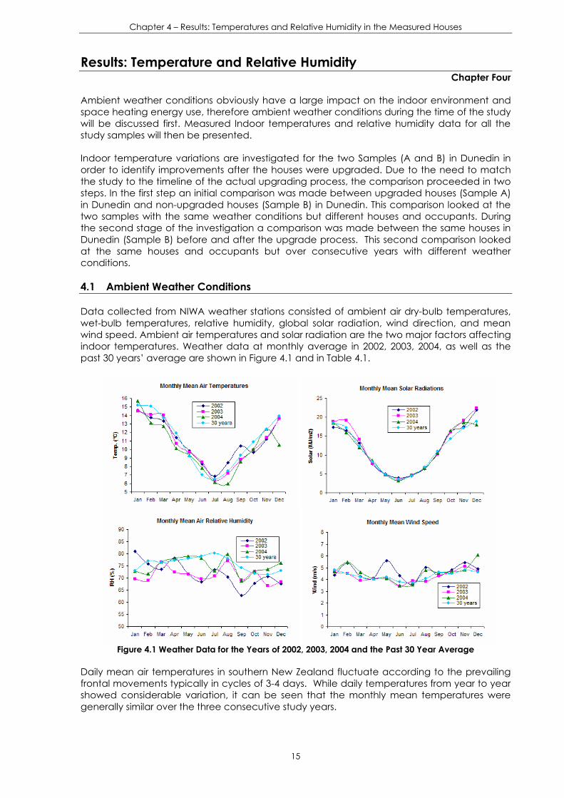
Chapter 4 – Results: Temperatures and Relative Humidity in the Measured Houses
15
Results: Temperature and Relative Humidity Chapter Four
Ambient weather conditions obviously have a large impact on the indoor environment and space heating energy use, therefore ambient weather conditions during the time of the study will be discussed first. Measured Indoor temperatures and relative humidity data for all the study samples will then be presented.
Indoor temperature variations are investigated for the two Samples (A and B) in Dunedin in order to identify improvements after the houses were upgraded. Due to the need to match the study to the timeline of the actual upgrading process, the comparison proceeded in two steps. In the first step an initial comparison was made between upgraded houses (Sample A) in Dunedin and non-upgraded houses (Sample B) in Dunedin. This comparison looked at the two samples with the same weather conditions but different houses and occupants. During the second stage of the investigation a comparison was made between the same houses in Dunedin (Sample B) before and after the upgrade process. This second comparison looked at the same houses and occupants but over consecutive years with different weather conditions.
4.1 Ambient Weather Conditions
Data collected from NIWA weather stations consisted of ambient air dry-bulb temperatures, wet-bulb temperatures, relative humidity, global solar radiation, wind direction, and mean wind speed. Ambient air temperatures and solar radiation are the two major factors affecting indoor temperatures. Weather data at monthly average in 2002, 2003, 2004, as well as the past 30 years’ average are shown in Figure 4.1 and in Table 4.1.
Figure 4.1 Weather Data for the Years of 2002, 2003, 2004 and the Past 30 Year Average
Daily mean air temperatures in southern New Zealand fluctuate according to the prevailing frontal movements typically in cycles of 3-4 days. While daily temperatures from year to year showed considerable variation, it can be seen that the monthly mean temperatures were generally similar over the three consecutive study years.
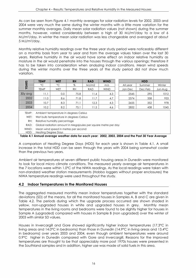
Chapter 4 – Results: Temperatures and Relative Humidity in the Measured Houses
16
As can be seen from Figure 4.1 monthly averages for solar radiation levels for 2002, 2003 and 2004 were very much the same during the winter months with a little more variation for the summer monthly averages. Daily mean solar radiation values (not shown) during the summer months, however, varied considerably between a high of 30 MJ/m2/day to a low of 6 MJ/m2/day. In winter the mean solar radiation was less changeable and averaged at about 5 MJ/m2/day.
Monthly relative humidity readings over the three year study period were noticeably different on a monthly basis from year to year and from the average values taken over the last 30 years. Relative humidity in the air would have some effect on indoor relative humidity as moisture in the air would penetrate into the houses through the various openings; therefore it has to be taken into consideration when analyzing indoor conditions. Mean wind speeds during the winter months over the three years of the study period did not show much variation.
TEMP WET RH RAD WIND HDD °C °C % MJ/m2 m/s All year Summer Winter
YEA
RS
TEMP WET RH RAD WIND Jan-Dec Dec-Feb Jun-Aug
30y avg 11.1 0.0 75.8 11.4 4.3 2545 295 1012 2002 11.0 8.6 71.8 11.7 4.7 2574 358 933 2003 10.7 8.3 71.1 12.3 4.3 2655 352 978 2004 10.2 8.2 75.1 11.5 4.6 2852 438 1045
TEMP: Ambient temperature in degrees Celsius WET: Wet bulb temperature in degrees Celsius
RH: Relative humidity percentage RAD: Global radiation amount in Megajoules per square metre per day
WIND: Mean wind speed in metres per second HDD: Heating Degree Days
Table 4.1 Annual average weather data for each year: 2002, 2003, 2004 and the Past 30 Year Average
A comparison of Heating Degree Days (HDD) for each year is shown in Table 4.1. A small increase in the total HDD can be seen through the years with 2004 being somewhat cooler than the previous two years.
Ambient air temperatures at seven different public housing areas in Dunedin were monitored to look for local micro climate conditions. The measured yearly average air temperatures in the 7 locations were within 1.0ºC of the NIWA readings. As the local readings were taken with non-standard weather station measurements (Hobbo loggers without proper enclosures) the NIWA temperature readings were used throughout the study.
4.2 Indoor Temperatures in the Monitored Houses
The aggregated measured monthly mean indoor temperatures together with the standard deviations (SD) of the means, for all the monitored houses in Samples A, B and C are given in Table 4.2. The periods during which the upgrade process occurred are shown shaded in yellow, non-upgraded houses in white and upgraded houses in grey. Monthly mean temperatures in the living rooms and bedrooms were found to be slightly higher for houses in Sample A (upgraded) compared with houses in Sample B (non upgraded) over the winter of 2003 with similar SD values.
Houses in Invercargill and Gore showed significantly higher indoor temperatures (17.3°C in living areas and 14.0°C in bedrooms) than those in Dunedin (14.9°C in living areas and 13.4°C in bedrooms) over years 2003 and 2004, even though ambient temperatures were around 0.9°C higher in Dunedin compared with Gore and Invercargill. Reasons for the improved temperatures are thought to be that appreciably more post 1970s houses were presented in the Southland samples and in addition, higher use was made of solid fuels in this area.

Chapter 4 – Results: Temperatures and Relative Humidity in the Measured Houses
17
Table 4.2 Measured Monthly Mean Indoor Temperatures for all monitored houses for Dunedin,
Invercargill and Gore showing Ambient Mean Temperature for each city
The monthly mean temperature variation for the houses in Sample A in Dunedin showed that the monthly average living rooms temperatures varied within about a 4°C range during summer but this increased to an 11°C range during winter, with a low median value of 13°C in July. The monthly mean temperature differences across the 3 samples for the bedrooms varied over a relatively small range, only about 1- 2°C during the year. As can be seen in Figure 4.2, the distribution patterns shifted to lower temperatures from summer to winter.
Living Areas - Indoor Temperatures for all monitored houses
5.06.07.08.09.0
10.011.012.013.014.015.016.017.018.019.020.021.022.0
2003 2004
Tem
per
atu
re C
GROUP A - LIVING GROUP B - LIVING GROUP C - INV - LIVING GROUP C - GORE - LIVING AM BIENT
Bedrooms - Indoor Temperatures for all monitored houses
5.06.07.08.09.0
10.011.012.013.014.015.016.017.018.019.020.021.022.0
2003 2004
Tem
per
atu
re C
GROUP A - BEDROOM GROUP B - BEDROOM GROUP C - INV - BEDROOM GROUP C - GORE - BEDROOM AM BIENT
Figure 4.2: Temperature variation for all monitored houses Samples A, B & C
for living rooms and bedrooms (2003 – 2004)
In terms of indoor temperature comfort levels, aggregated hourly temperature data showed that 18°C was too difficult to reach for most of the public housing during the year. Monthly histograms for all houses in Sample A and B in Dunedin for winter time are shown in Figure 4.3.
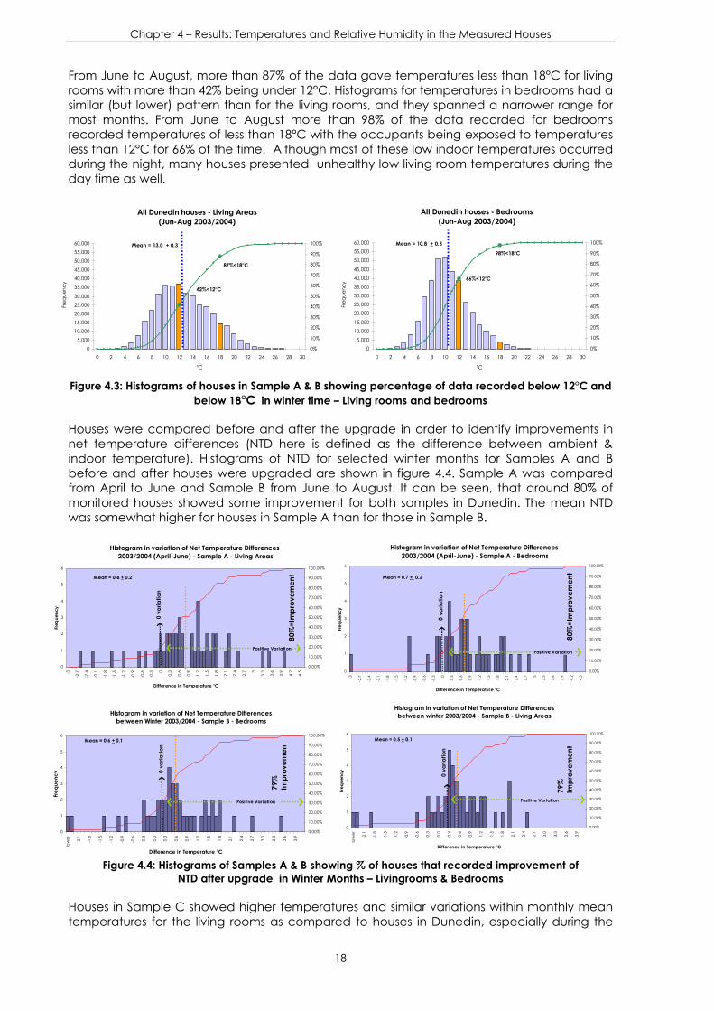
Chapter 4 – Results: Temperatures and Relative Humidity in the Measured Houses
18
From June to August, more than 87% of the data gave temperatures less than 18°C for living rooms with more than 42% being under 12°C. Histograms for temperatures in bedrooms had a similar (but lower) pattern than for the living rooms, and they spanned a narrower range for most months. From June to August more than 98% of the data recorded for bedrooms recorded temperatures of less than 18°C with the occupants being exposed to temperatures less than 12ºC for 66% of the time. Although most of these low indoor temperatures occurred during the night, many houses presented unhealthy low living room temperatures during the day time as well.
All Dunedin houses - Living Areas(Jun-Aug 2003/2004)
42%<12°C
87%<18°C
05,000
10,00015,00020,00025,00030,000
35,00040,00045,00050,00055,00060,000
0 2 4 6 8 10 12 14 16 18 20 22 24 26 28 30
°C
Freq
uenc
y
0%
10%
20%
30%
40%
50%
60%
70%
80%
90%
100%Mean = 13.0 + 0.3
All Dunedin houses - Bedrooms(Jun-Aug 2003/2004)
66%<12°C
98%<18°C
05,000
10,00015,000
20,00025,00030,00035,00040,00045,000
50,00055,00060,000
0 2 4 6 8 10 12 14 16 18 20 22 24 26 28 30
°C
Freq
uenc
y0%
10%
20%
30%
40%
50%
60%
70%
80%
90%
100%Mean = 10.8 + 0.3
Figure 4.3: Histograms of houses in Sample A & B showing percentage of data recorded below 12°C and
below 18°C in winter time – Living rooms and bedrooms
Houses were compared before and after the upgrade in order to identify improvements in net temperature differences (NTD here is defined as the difference between ambient & indoor temperature). Histograms of NTD for selected winter months for Samples A and B before and after houses were upgraded are shown in figure 4.4. Sample A was compared from April to June and Sample B from June to August. It can be seen, that around 80% of monitored houses showed some improvement for both samples in Dunedin. The mean NTD was somewhat higher for houses in Sample A than for those in Sample B.
Histogram in variation of Net Temperature Differences 2003/2004 (April-June) - Sample A - Living Areas
0
1
2
3
4
5
6
-3
-2.7
-2.4
-2.1
-1.8
-1.5
-1.2
-0.9
-0.6
-0.3 0
0.3
0.6
0.9
1.2
1.5
1.8
2.1
2.4
2.7 3
3.3
3.6
3.9
4.2
4.5
Difference in Temperature °C
Freq
uenc
y
0.00%
10.00%
20.00%
30.00%
40.00%
50.00%
60.00%
70.00%
80.00%
90.00%
100.00%
0 va
riatio
n
80%
=Im
prov
emen
t
Positive Variation
Mean = 0.8 + 0.2
Histogram in variation of Net Temperature Differences 2003/2004 (April-June) - Sample A - Bedrooms
0
1
2
3
4
5
6
-3
-2.7
-2.4
-2.1
-1.8
-1.5
-1.2
-0.9
-0.6
-0.3 0
0.3
0.6
0.9
1.2
1.5
1.8
2.1
2.4
2.7 3
3.3
3.6
3.9
4.2
4.5
Difference in Temperature °C
Freq
uenc
y
0.00%
10.00%
20.00%
30.00%
40.00%
50.00%
60.00%
70.00%
80.00%
90.00%
100.00%
0 va
riatio
n
80%
=Im
prov
emen
t
Positive Variation
Mean = 0.7 + 0.2
Histogram in variation of Net Temperature Differences
between Winter 2003/2004 - Sample B - Bedrooms
0
1
2
3
4
5
6
low
er -2.1
-1.8
-1.5
-1.2
-0.9
-0.6
-0.3 0.0
0.3
0.6
0.9
1.2
1.5
1.8
2.1
2.4
2.7
3.0
3.3
3.6
3.9
Difference in Temperature °C
Freq
uenc
y
0.00%
10.00%
20.00%
30.00%
40.00%
50.00%
60.00%
70.00%
80.00%
90.00%
100.00%
0 va
riatio
n
79%
Impr
ovem
ent
Positive Variation
Mean = 0.6 + 0.1
Histogram in variation of Net Temperature Differences between winter 2003/2004 - Sample B - Living Areas
0
1
2
3
4
5
6
low
er -2.1
-1.8
-1.5
-1.2
-0.9
-0.6
-0.3 0.0
0.3
0.6
0.9
1.2
1.5
1.8
2.1
2.4
2.7
3.0
3.3
3.6
3.9
Difference in Temperature °C
Freq
uenc
y
0.00%
10.00%
20.00%
30.00%
40.00%
50.00%
60.00%
70.00%
80.00%
90.00%
100.00%
0 va
riatio
n
79%
Impr
ovem
ent
Positive Variation
Mean = 0.5 + 0.1
Figure 4.4: Histograms of Samples A & B showing % of houses that recorded improvement of
NTD after upgrade in Winter Months – Livingrooms & Bedrooms
Houses in Sample C showed higher temperatures and similar variations within monthly mean temperatures for the living rooms as compared to houses in Dunedin, especially during the

Chapter 4 – Results: Temperatures and Relative Humidity in the Measured Houses
19
winter months. There were similar average bedroom temperatures and variances recorded over all the 3 samples A, B and C.
Exposure to Indoor Temperatures
As other researches have noted (Chapman et. al. 2004) it is not so much the absolute indoor temperatures presented that is important to health concerns as the exposure of occupants to periods of low (or high) temperatures. In this respect exposure in bedrooms is problematic due to the possibility of considerably higher personal “ambient” temperatures being the norm while occupants are actually in bed under high R value blankets and bedding. To this extent the research has differentiated between exposure to indoor temperatures during “awake-hours” (8:00 am to 10:00 pm) and “sleep-hours” (10:00 pm to 8:00 am).
The majority of occupants of the Housing New Zealand Corporation residences were unemployed, low-income people and they often occupied the homes during the day. Indoor temperatures in the living rooms during “awake-hours” (AH) and in bedrooms during “sleep-hours” (SH) would represent a more realistic “exposure” of the occupants to indoor temperatures. As heating was mostly put in place during “awake-hours” it is likely that the “awake-hours” temperatures should be greater than the 24 hour averages. This in fact is what the survey found.
“Awake-hours” temperatures were generally higher than the 24 hour average for living areas while the “sleep-hours” temperatures were generally lower than the 24 hour average for bedrooms. The monthly “awake-hours” mean temperatures in living rooms for houses in Sample A for the winter 2003 was about 0.6°C higher than the 24 hour average. The monthly “sleep-hours” mean temperature in bedrooms was about 0.1°C lower than the 24 hour average in winter and 0.3°C lower in summer. Monthly mean “awake-hours” and “sleep-hours” temperatures for each of the samples are shown in Table 4.3.
Houses in Sample B (before being upgraded) had 0.2°C higher mean temperature in living rooms during “awake-hours” compared with the 24 hour average for winter 2003. “Sleep-hours” temperatures were 1.0°C lower than the 24 hour average in winter for the bedrooms. In summer time living rooms were 0.3°C higher than the 24 hour average and bedrooms were 0.5°C lower than the 24 hour average.
Table 4.3 Monthly Mean “awake-hours” (AH) Temperatures in Living Room and “sleep-hours” (SH) Temperature in Bedroom for All the Monitored Houses in 2003. (Dnd = Dunedin, Inv = Invercargill)
This analysis suggests that houses in Sample A were able to maintain better indoor temperatures throughout the night in bedrooms while providing higher temperatures during the day in the living areas as compared with houses in Sample B.

Chapter 4 – Results: Temperatures and Relative Humidity in the Measured Houses
20
About 83% of the measured hourly living room temperatures in houses in Sample A were lower than 18°C and 33% (4.5 hours) were lower than 12°C during the “awake-hours” in winter. The bedrooms during “sleep-hours” were even cooler with 97% being lower than 18°C and 69% (or 7 hours) lower than 12°C over the winter months. In terms of hours when the occupant could be exposed to low indoor temperatures in the upgraded houses in Dunedin, there were around 4.5 hours each day in winter, in the living rooms, during “awake-hours” and 7.0 hours in the bedrooms during “sleep-hours” when people could be exposed to indoor temperatures of less than 12°C. In total this amounts to 11.5 hours or 48% of the time that the occupants could be exposed to temperatures less than 12°C during the winter months of June to August inclusive.
In addition, the absolute minimum temperature recorded for each house in Sample B only was also analyzed. Bedrooms recorded an average minimum temperature (the individual household minimums averaged over the entire sample of 50 houses), during “sleep-hours”, for the winter months (June to August) of 5°C for 2003 and 5.3°C for 2004. Living areas recorded during “awake-hours” a minimum temperature of 5.3°C in 2003 and 5.4°C in 2004 (see figure 4.5). The above analysis suggests that the upgrade program had little impact in improving these very low absolute temperatures and that during winter months, people could still be exposed to very low indoor temperatures even after houses were upgraded.
Histogram of absolute minimum temperature redorded inSample B - bedrooms during "sleep hours"
Winter (2003 vs 2004)
0
1
2
3
4
5
6
7
8
0.0
0.5
1.0
1.5
2.0
2.5
3.0
3.5
4.0
4.5
5.0
5.5
6.0
6.5
7.0
7.5
8.0
8.5
9.0
9.5
10.0
10.5
11.0
Mor
e
Temperature ºC
Freq
uenc
y
2003 BEDROOM SLEEP HOURS
2003 BEDROOM SLEEP HOURS
Mea
n 5.
0Cº
(200
3)
Mea
n 5.
3Cº
(200
4)
Histogram of absolute minimum temperature redorded in Sample B - livingareas during "awake hours"
Winter (2003 vs 2004)
0
1
2
3
4
5
6
7
8
0.0
0.5
1.0
1.5
2.0
2.5
3.0
3.5
4.0
4.5
5.0
5.5
6.0
6.5
7.0
7.5
8.0
8.5
9.0
9.5
10.0
10.5
11.0
Mor
e
Temperature ºC
Freq
uenc
y
2003 LIVING AREAS - AWAKE HOURS
2004 LIVING AREAS - AWAKE HOURS
Mea
n 5.
3Cº
(200
3)
Mea
n 5.
4Cº
(200
4)
Figure 4.5 Histograms of absolute minimum temperatures for bedrooms during “sleep-hours” and living areas during “awake-hours” in Sample B houses during winter months (2003 vs. 2004)
However, because the second year was slightly colder than the first year, the minimum net temperature differences (the difference between indoor and ambient temperature) improvement after the upgrade was also analyzed. The minimum net temperature differences were almost always negative for all sample houses, indicating that the indoor temperature was on some occasion actually lower than ambient,. This situation would be expected to occur early in the morning when ambient temperatures rise faster than indoor temperatures due to the thermal inertia of the building. An improvement in minimum net temperature differences for the bedrooms during “sleep-hours” after the upgrade was found in 90% of the sample with an average of -3.9°C NTD found for the winter of 2003 (non-upgraded) and -2°C NTD found for the winter of 2004 (upgraded). Living areas however, did not show the same improvement during “awake-hours”, with an average of -3.7°C NTD for the winter of 2003 (non-upgraded) and -4.5°C NTD for the winter of 2004 (upgraded). These findings would be expected as insulation can have little effect on indoor temperatures if there is no space heating, no internal gains, no conduction gains and no sunshine; as in the living areas during the coldest part of the early morning. The bedrooms on the other hand would have at least the internal gain of the occupants. Small gains were observed for the bedrooms but still the absolute temperature regimes observed were extremely low.
Indoor temperature variation due to differences in house structure and vintage
The post-1970s houses were found to be significantly warmer than the other two construction periods especially for the living area (see Figure 4.6). Mean temperatures of 16.4°C in winter
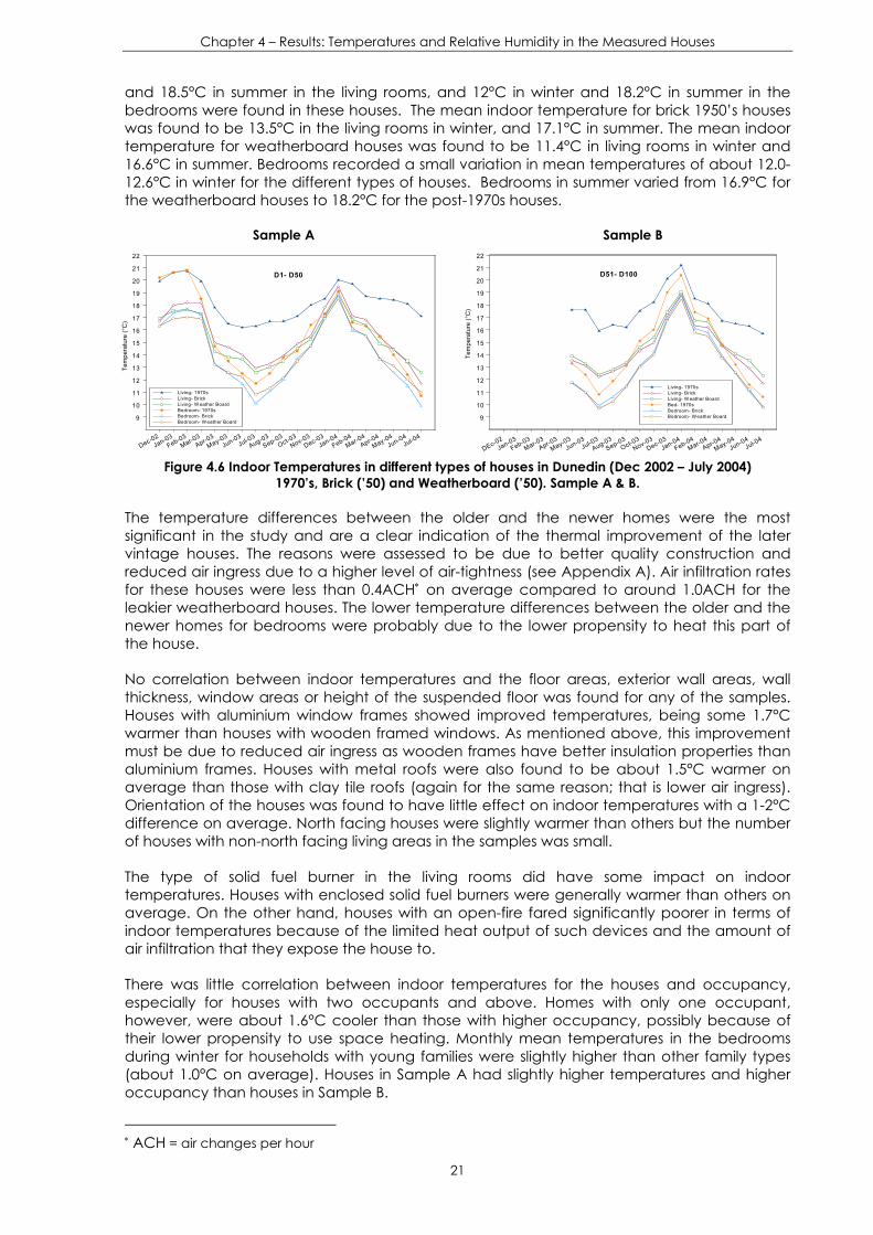
Chapter 4 – Results: Temperatures and Relative Humidity in the Measured Houses
21
and 18.5°C in summer in the living rooms, and 12°C in winter and 18.2°C in summer in the bedrooms were found in these houses. The mean indoor temperature for brick 1950’s houses was found to be 13.5°C in the living rooms in winter, and 17.1°C in summer. The mean indoor temperature for weatherboard houses was found to be 11.4°C in living rooms in winter and 16.6°C in summer. Bedrooms recorded a small variation in mean temperatures of about 12.0-12.6°C in winter for the different types of houses. Bedrooms in summer varied from 16.9°C for the weatherboard houses to 18.2°C for the post-1970s houses.
Sample A Sample B
Dec-02Jan-03
Feb-03Mar-03
Apr-03May-03
Jun-03Jul-03
Aug-03Sep-03
Oct-03Nov-03
Dec-03Jan-04
Feb-04Mar-04
Apr-04May-04
Jun-04Jul-04
Tem
pera
ture
(°C
)
9
10
11
12
13
14
15
16
17
18
19
20
21
22
Living- 1970sLiving- BrickLiving- W eather BoardBedroom- 1970sBedroom- BrickBedroom- W eather Board
D1- D50
DEc-02Jan-03
Feb-03Mar-03
Apr-03May-03
Jun-03Jul-03
Aug-03Sep-03
Oct-03Nov-03
Dec-03Jan-04
Feb-04Mar-04
Apr-04May-04
Jun-04Jul-04
Tem
pera
ture
(°C
)
9
10
11
12
13
14
15
16
17
18
19
20
21
22
Living- 1970sLiving- BrickLiving- W eather BoardBed- 1970sBedroom- BrickBedroom- Weather Board
D51- D100
Figure 4.6 Indoor Temperatures in different types of houses in Dunedin (Dec 2002 – July 2004)
1970’s, Brick (’50) and Weatherboard (’50). Sample A & B.
The temperature differences between the older and the newer homes were the most significant in the study and are a clear indication of the thermal improvement of the later vintage houses. The reasons were assessed to be due to better quality construction and reduced air ingress due to a higher level of air-tightness (see Appendix A). Air infiltration rates for these houses were less than 0.4ACH∗ on average compared to around 1.0ACH for the leakier weatherboard houses. The lower temperature differences between the older and the newer homes for bedrooms were probably due to the lower propensity to heat this part of the house.
No correlation between indoor temperatures and the floor areas, exterior wall areas, wall thickness, window areas or height of the suspended floor was found for any of the samples. Houses with aluminium window frames showed improved temperatures, being some 1.7°C warmer than houses with wooden framed windows. As mentioned above, this improvement must be due to reduced air ingress as wooden frames have better insulation properties than aluminium frames. Houses with metal roofs were also found to be about 1.5°C warmer on average than those with clay tile roofs (again for the same reason; that is lower air ingress). Orientation of the houses was found to have little effect on indoor temperatures with a 1-2°C difference on average. North facing houses were slightly warmer than others but the number of houses with non-north facing living areas in the samples was small.
The type of solid fuel burner in the living rooms did have some impact on indoor temperatures. Houses with enclosed solid fuel burners were generally warmer than others on average. On the other hand, houses with an open-fire fared significantly poorer in terms of indoor temperatures because of the limited heat output of such devices and the amount of air infiltration that they expose the house to.
There was little correlation between indoor temperatures for the houses and occupancy, especially for houses with two occupants and above. Homes with only one occupant, however, were about 1.6°C cooler than those with higher occupancy, possibly because of their lower propensity to use space heating. Monthly mean temperatures in the bedrooms during winter for households with young families were slightly higher than other family types (about 1.0°C on average). Houses in Sample A had slightly higher temperatures and higher occupancy than houses in Sample B.
∗ ACH = air changes per hour

Chapter 4 – Results: Temperatures and Relative Humidity in the Measured Houses
22
4.3 First Comparison of the Measured Indoor Temperatures between Sample A (upgraded) & Sample B (non upgraded) in 2003
Houses participating in the upgrade program were upgraded over a time span of 5 months during the year of the upgrade. The aim was to compare “upgraded” vs. “non-upgraded” houses to be able to identify any improvement in indoor temperatures due to the upgrade. In this case, houses in Sample A were gradually upgraded from January to May 2003. Houses in Sample B were upgraded during the following year from October 2003 to February 2004. The temperature comparisons take into account the progress of the upgrade program, in two stages. In both stages, houses that were upgraded were considered individually in each month and the percentage of houses taking part in the comparison is given at the bottom of each table (4.6 and 4.7). Net temperature differences (NTD) were considered for the comparisons; they represent the difference between indoor and ambient temperatures, with the ambient temperatures as measured by NIWA.
Monthly mean temperatures in the living rooms and bedrooms for the two Samples (A and B) of houses in 2003 had similar standard deviation values for most months (see Table 4.1). In the summer months, similar indoor temperatures between Sample A and Sample B were recorded for the whole house, while in winter months lower temperatures were presented in bedrooms.
The indoor temperature variations over the entire monitoring period are shown in Figure 4.7. Houses in Sample A showed higher indoor temperatures than those of Sample B, both before and after Sample B was upgraded. Reasons for this could include the small structural differences of the sample, including that more weatherboard houses were presented in Sample B (48% compared with 40%), higher occupancy level and/or behavioural differences.
Figure 4.7: Monthly Mean Temperatures Upgraded vs. Non-upgraded Houses
in Living Rooms and Bedrooms (2003 – 2004).
During the first winter of the comparison between Sample A and Sample B, the differences between the means of the two individual samples were 0.6 + 0.1°C for the living rooms, and 0.7° + 0.2°C for the bedrooms, with Sample A being higher than Sample B in both cases. The aggregated average daily mean temperatures for the living rooms were 13.2 ± 0.1°C for the upgraded homes and 12.6 ± 0.1°C for the non-upgraded homes for the two months in winter 2003 (July and August). Daily mean bedroom temperatures closely followed ambient air temperature variations as can be seen in Figure 4.8.

Chapter 4 – Results: Temperatures and Relative Humidity in the Measured Houses
23
Figure 4.8 Comparison of Daily Mean Temperatures in Living Rooms and Bedrooms between Upgraded
and Non-upgraded Houses in Dunedin during the Winter of 2003
The temperatures differences between Sample A and Sample B houses for the monitoring period are shown in Table 4.4. This data suggests that only the living areas were actively heated during winter. It can also be noted that after houses were upgraded, there was a slight increase in NTD, suggesting that the insulation was able to retain some of the heat produced from space heating. It can also be seen that houses in Sample A had higher net temperatures differences than those in Sample B after the upgrade, indicating that the houses in Sample A were on average warmer than with Sample B.
Table 4.4 Indoor/Outdoor Temperatures Differences for Sample A & B Houses in 2003 and 2004
Taking into account the average NTD for both winters for Sample A (already upgraded during both winters), the difference in temperatures for Sample B before and after that sample was upgraded, was calculated. This difference shows that Sample A was warmer than Sample B by 0.3°C in the living rooms and 0.4°C in the bedrooms. This difference was presumed to be

Chapter 4 – Results: Temperatures and Relative Humidity in the Measured Houses
24
due to both the structural and behavioural differences between the two samples. Considering these differences, we can then compare the temperatures recorded during the first winter when Sample A was upgraded and Sample B was not upgraded. The results show that an increase in indoor temperature of 0.6°C occurred in both the living rooms and the bedrooms due to the upgrade (see Table 4.5).
Table 4.5 Improvement in Net Temperature Difference - Sample A vs. Sample B
4.4 Second Comparison of the Measured Indoor Temperatures: for the same Sample of houses before and after upgrade
Sample A (2003 & 2004)
The measured monthly mean temperatures for Sample A houses in the first half of 2003 and 2004 together with the ambient temperature for this period is shown in the Table 4.6.
The NTD’s for the summer months of January to March were similar before and after the upgrade. The winter months of April to June showed an increase in the mean NTD of between 0.9-0.7°C in both the living areas and the bedrooms after the insulation. The period April to June could only be taken as representative of the cooler months as all houses in Sample A had been upgraded by the end of this period. July then presented similar NTD after all the houses were upgraded.
Table 4.6 Comparison of the Measured Monthly Mean Indoor Temperature
for houses in Sample A (D1- D50) in 2003 & 2004. (UCL=Upper Confidence Level, LCL=Lower Confidence Level)
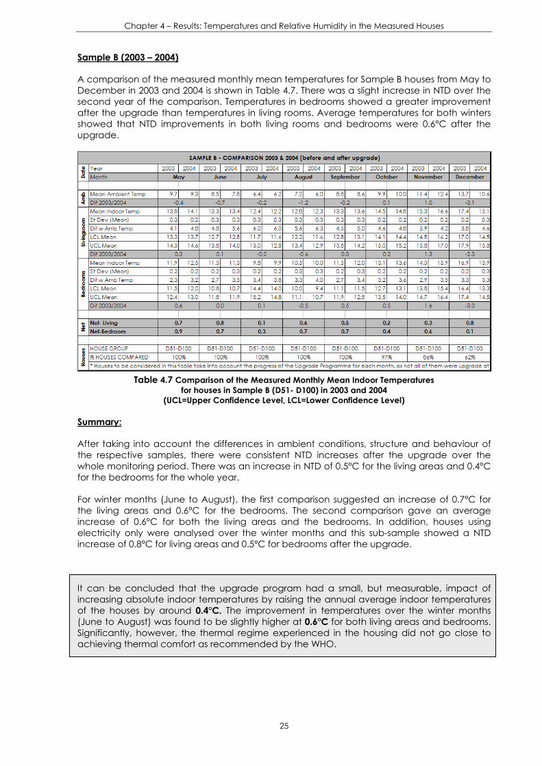
Chapter 4 – Results: Temperatures and Relative Humidity in the Measured Houses
25
Sample B (2003 – 2004)
A comparison of the measured monthly mean temperatures for Sample B houses from May to December in 2003 and 2004 is shown in Table 4.7. There was a slight increase in NTD over the second year of the comparison. Temperatures in bedrooms showed a greater improvement after the upgrade than temperatures in living rooms. Average temperatures for both winters showed that NTD improvements in both living rooms and bedrooms were 0.6°C after the upgrade.
Table 4.7 Comparison of the Measured Monthly Mean Indoor Temperatures for houses in Sample B (D51- D100) in 2003 and 2004
(UCL=Upper Confidence Level, LCL=Lower Confidence Level)
Summary:
After taking into account the differences in ambient conditions, structure and behaviour of the respective samples, there were consistent NTD increases after the upgrade over the whole monitoring period. There was an increase in NTD of 0.5°C for the living areas and 0.4°C for the bedrooms for the whole year.
For winter months (June to August), the first comparison suggested an increase of 0.7°C for the living areas and 0.6°C for the bedrooms. The second comparison gave an average increase of 0.6°C for both the living areas and the bedrooms. In addition, houses using electricity only were analysed over the winter months and this sub-sample showed a NTD increase of 0.8°C for living areas and 0.5°C for bedrooms after the upgrade.
It can be concluded that the upgrade program had a small, but measurable, impact of increasing absolute indoor temperatures by raising the annual average indoor temperatures of the houses by around 0.4°C. The improvement in temperatures over the winter months (June to August) was found to be slightly higher at 0.6°C for both living areas and bedrooms. Significantly, however, the thermal regime experienced in the housing did not go close to achieving thermal comfort as recommended by the WHO.

Chapter 4 – Results: Temperatures and Relative Humidity in the Measured Houses
26
4.5 24 Hour Indoor Temperatures Profiles
Energy use data (see Chapter 5) suggested that the households in the study samples heated rooms intermittently rather than continuously, thus the time dependant behaviour of the indoor temperature was considered.
The 24 hour indoor temperature profiles when averaged across the relevant Samples (A and B) for living areas and bedrooms (Dunedin houses only) are compared with the 24 hour average ambient temperature profiles for January and June for 2003 and 2004 in order to analyse time dependant improvements in the houses after the upgrades. Here the 24 hour ambient temperature profiles were calculated by averaging the NIWA measured hourly profiles for each day of the month.
January 2003-2004 data were analysed for houses in Sample A, representing a typical summer profile. As can be seen in Figure 4.9, a difference was observed between the temperatures in the living rooms and the bedrooms beginning at 10:00 a.m. This difference is driven by solar radiation and internal energy usage in the living areas. The peak temperatures in both rooms occurred at around 7:00 p.m. after which the rooms cooled down to the same temperatures by the next morning at 8:00 a.m. The thermal inertia of the house introduced a clear lag effect, of around 5 hours, between peak indoor temperatures and peak ambient temperatures. As it can be seen, only small differences occur between the bedrooms and the living areas in summer time, most likely due to the predominance of north facing living area windows. There is no sign of substantial internal heat gain from space heating, as might expected for this time of the year.
In winter there was a far greater divergence in temperatures between the (unheated) bedrooms and the (heated) living areas. In addition the NTDs were larger in the living areas which indicated space heating energy was applied sometime between 10:00 a.m. to 8:00 p.m. Houses in Sample A and B were compared for the month of June 2003 and 2004 to identify improvements in NTD variations due to the upgrade. Note that not all the houses in each sample could be included in the comparison due to the actual scheduling of the upgrade. The month of June was used to represent winter conditions with the advantage of this month having similar mean energy consumption for both samples for both years. These results are shown in Figure 4.10.
Figure 4.9 24 Hour Temperature Profiles for houses in Sample A in January 2003 & 2004
As can be seen from these profiles for the living areas, the temperature increases due to solar radiation and internal gain from around 9:00 a.m., then peaking around 5:00 p.m. after which solar radiation ceases and both indoor and ambient temperatures begins to decrease. Space heating generally starts around this time (5:00 p.m.) in living areas, and peaking between 9:00 p.m. and 10:00 p.m. (as indicated by the peak in net temperature differences) after which the rooms cool down over night. It is important to note that after heating is stopped, the period of cooling down for both years follows a separate curve. In 2003, before insulation, the cooling down occurs at a faster rate than during the following year (after the upgrade). This improvement provides a larger net difference in temperatures for the living areas, but
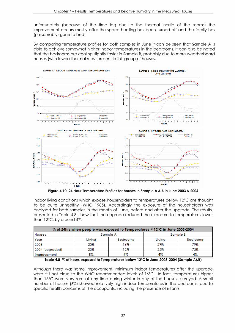
Chapter 4 – Results: Temperatures and Relative Humidity in the Measured Houses
27
unfortunately (because of the time lag due to the thermal inertia of the rooms) the improvement occurs mostly after the space heating has been turned off and the family has (presumably) gone to bed.
By comparing temperature profiles for both samples in June it can be seen that Sample A is able to achieve somewhat higher indoor temperatures in the bedrooms. It can also be noted that the bedrooms are cooling slightly faster in Sample B, probably due to more weatherboard houses (with lower) thermal mass present in this group of houses.
Figure 4.10 24 Hour Temperature Profiles for houses in Sample A & B in June 2003 & 2004
Indoor living conditions which expose householders to temperatures bellow 12°C are thought to be quite unhealthy (WHO 1985). Accordingly the exposure of the householders was analysed for both samples in the month of June, before and after the upgrade. The results, presented in Table 4.8, show that the upgrade reduced the exposure to temperatures lower than 12°C, by around 4%.
Table 4.8 % of hours exposed to Temperatures below 12°C in June 2003-2004 (Sample A&B)
Although there was some improvement, minimum indoor temperatures after the upgrade were still not close to the WHO recommended levels of 16°C. In fact, temperatures higher than 16°C were very rare at any time during winter in any of the houses surveyed. A small number of houses (6%) showed relatively high indoor temperatures in the bedrooms, due to specific health concerns of the occupants, including the presence of infants.

Chapter 4 – Results: Temperatures and Relative Humidity in the Measured Houses
28
4.6 Relative Humidity Results
Relative humidity is a measure of the water vapour content of the air at a given temperature. The amount of moisture in the air is compared with the maximum amount that the air could contain at the same temperature and expressed as a percentage. In general a rise of indoor temperatures will result in the reduction of relative humidity in the room. Relative humidity results were only collected for the houses monitored in detail (i.e. 22 houses in Sample A and 8 houses in Sample C)
Daily mean relative humidity in the living rooms followed similar changes to the ambient air humidity, as can be seen in Figure 4.11. Unlike indoor temperatures, relative humidity did not show any marked seasonal variation. The daily mean relative humidity was about 60% ±6% in the living rooms and 71% ±10% in the ambient air over the whole year. The difference between the average daily mean relative humidity between the indoor and outdoor air was 12% ±7% in 2003.
The mean indoor to outdoor relative humidity difference was 9.0% ±2% from December 2002 to May 2003 and 15% ±3% from July 2003 to July 2004. Thus there was about a 6% reduction in relative humidity in indoor air after the houses were upgraded.
Dec-02Jan-03
Feb-03Mar-03
Apr-03May-03
Jun-03Jul-03
Aug-03Sep-03
Oct-03Nov-03
Dec-03Jan-04
Feb-04Mar-04
Apr-04May-04
Jun-04Jul-04
Mean
40
45
50
55
60
65
70
75
80
RH
(%)
Ambient Air
Figure 4.11 Monthly mean relative humidity (RH) for D1-D22 Houses from December 2002 to July 2004
Plots of the average 24 hour relative humidity variation for the 22 houses in Dunedin in January and July 2003 are shown in Figure 4.12. Mean relative humidity showed profiles without much change during the day. Indoor relative humidity was very close to the ambient air relative humidity in summer as people might be expected to open windows more often at this time of the year. The mean indoor to outdoor difference was 16% ±5% in winter. As might be expected, in general, warmer houses showed lower average relative humidity in the living rooms than cooler houses.
RH of D1- D22 in January 2003
Living Room
Ambient Air
0
10
20
30
40
50
60
70
80
90
100
0:00
1:00
2:00
3:00
4:00
5:00
6:00
7:00
8:00
9:00
10:0
011
:00
12:0
013
:00
14:0
015
:00
16:0
017
:00
18:0
019
:00
20:0
021
:00
22:0
023
:00
Time
RH (%
)
RH of D1- D22 in July 2003
Living Room
Ambient Air
0
10
20
30
40
50
60
70
80
90
100
0:00
1:00
2:00
3:00
4:00
5:00
6:00
7:00
8:00
9:00
10:0
011
:00
12:0
013
:00
14:0
015
:00
16:0
017
:00
18:0
019
:00
20:0
021
:00
22:0
023
:00
Time
RH (%
)
Figure 4.12: The 24 Hour Mean Relative Humidity (RH) Changes for D1- D22 Houses in January and July 2003

Chapter 4 – Results: Temperatures and Relative Humidity in the Measured Houses
29
Indoor air temperatures below 16°C and relative humidity above 65% impose additional hazards to occupants’ health (WHO 1985). Relative humidity above 70% on cold surfaces can start the growth of mould in homes where there is lack of sufficient ventilation. Condensation normally appears on cold surfaces where local temperatures drop to below the air dew point. A monthly comparison between the ambient air and the indoor air regarding the hourly relative humidity data above 70% RH from January 2003 to July 2004 is given in Figure 4.13. This shows a clear reduction of the chance of indoor relative humidity over 70% after all houses were upgraded in June 2003. The average percentages of the measured hourly data of indoor relative humidity over 70% were 23% from January to May 2003 (before upgrade) and 11% from July 2003 to July 2004 (after upgrade). There was about a 12% reduction in the occurrence of indoor air relative humidity reaching over 70% after houses were upgraded.
0%
10%
20%
30%
40%
50%
60%
70%
80%
90%
Jan-
03Fe
b-03
Mar
-03
Apr
-03
May
-03
Jun-
03Ju
l-03
Aug
-03
Sep
-03
Oct
-03
Nov
-03
Dec
-03
Jan-
04Fe
b-04
Mar
-04
Apr
-04
May
-04
Jun-
04Ju
l-04
% o
f RH
Ove
r 70
%
Indoor MeanAmbient Air
Figure 4.13 Comparison of Mean % of hourly RH data exceeded 70% RH
between the Ambient Air and the Indoor Air (before and after the upgrade) for D1-D22 Houses

Chapter 5 – Results: Energy Use in the Study Houses
30
Results: Energy Use Chapter Five
Energy consumption for electricity, solid fuel and LPG was obtained for all the study houses. Electricity usage was obtained in several forms; firstly from the householder and/or read from the meter box, secondly from the supply retailer as historical records and thirdly as 20 minute samples from data loggers attached to the meter box. Non-electricity consumption was obtained from the householder. Data analysis of energy usage for the study houses was conducted by first examining the historical household electricity consumption of all the upgraded houses to get the household monthly means and compute the standard deviations for each sample. This data was then used for the comparison of energy use.
The measured household electricity consumption data for the houses monitored in detail was analyzed both on a monthly basis and on a 24 hour basis (Shen M. 2004). The measured electricity use for water heating for all houses was analyzed to obtain the monthly and yearly mean energy used for hot water production. The monthly energy use for solid fuel and LPG use was analyzed from occupant reported data.
5.1 Household Electricity Usage
Measured Household Electricity Consumption in the 30 Detailed Monitored Houses
The sample houses in Dunedin consumed more electrical energy than those in Invercargill and Gore in the period form December 2002 to July 2004 as can be seen in Figure 5.1. Houses in Gore exhibited a lower variation in electricity use as solid fuel for space heating in winter dominated.
Dec-02Jan-03
Feb-03Mar-03
Apr-03May-03
Jun-03Jul-03
Aug-03Sep-03
Oct-03Nov-03
Dec-03Jan-04
Feb-04Mar-04
Apr-04May-04
Jun-04Jul-04
0
200
400
600
800
1000
1200
1400
1600
1800
2000
2200
kWh
D1- D22 Houses in Dunedin
Mean
Dec-02Jan-03
Feb-03Mar-03
Apr-03May-03
Jun-03Jul-03
Aug-03Sep-03
Oct-03Nov-03
Dec-03Jan-04
Feb-04Mar-04
Apr-04May-04
Jun-04Jul-04
Mean
0
200
400
600
800
1000
1200
1400
1600
1800
2000
2200
kWh
5 Sample Houses in Invercargill
Dec-02Jan-03
Feb-03Mar-03
Apr-03May-03
Jun-03Jul-03
Aug-03Sep-03
Oct-03
Nov-03Dec-03
Jan-04Feb-04
Mar-04Apr-04
May-04Jun-04
Jul-04
Mean
0
200
400
600
800
1000
1200
1400
1600
1800
2000
2200
kWh
3 Sample Houses in Gore
Figure 5.1 Monthly Electricity Consumption for the 30 Detailed Monitored Houses in Dunedin, Invercargill
and Gore from December 2002 to July 2004
As might be expected, more electricity was consumed in the colder months from April to September because of space heating requirements, which peaked in July. The measured 24 hour mean monthly household electricity load patterns for the 22 houses in Dunedin monitored in 2003 are shown in Figure 5.2. The profiles show peaks in the morning around 9:00 am and between 7:00 pm and 9:00 pm. Similar profiles were presented over the summer months. High electricity use occurred during morning (10:00 am) and evenings (6:00 pm) for most houses in summer. The household electricity use in May 2003 showed an unusual profile with sharp peaks occurring in the early morning and the late evening. The reason was found to be the high power draw of water heating at that time due to the retailers’ ripple control of water heating in response to a perceived power shortage in the early winter.
The historical electricity consumption data showed electricity use for water heating was relatively constant throughout the year. Electricity consumption was least during the month of February.
By taking household energy use in February as the non-climate dependant base load for the year, the seasonal energy use (presumed to be mostly for space heating) is shown in Figure 5.3 for January to July 2003. January and March showed similar patterns of electricity use to the base load in February. Increased energy use started in April and peaked in July. Home
Elec
trici
ty C
onsu
mpt
ion
(kW
h)

Chapter 5 – Results: Energy Use in the Study Houses
31
heating was most often applied during evenings in winter. The areas between the monthly curves and the x axis give the monthly net increase of energy use (note the ripple control peaks for hot water usage during May 2003, which was not filtered out, after subtracting the non seasonal electricity consumption). Surprisingly, total electricity consumption during weekends, when most occupants would be at home, was similar to weekdays indicating a relatively high occupancy during the week as well. Extra energy was, however, used at midday instead of evenings during the weekends.
0.00.10.20.30.40.50.60.70.80.91.01.11.21.31.41.51.61.71.81.92.02.12.22.32.4
0:00
1:00
2:00
3:00
4:00
5:00
6:00
7:00
8:00
9:00
10:0
0
11:0
0
12:0
0
13:0
0
14:0
0
15:0
0
16:0
0
17:0
0
18:0
0
19:0
0
20:0
0
21:0
0
22:0
0
23:0
0Time
kW
JanFebMarAprMayJunJulAugSepOctNovDec
Figure 5.2 The 24 Hour Monthly Mean Household Electricity Load Patterns for D1-D22 Houses in
Dunedin in 2003
-0.1
0.0
0.1
0.2
0.3
0.4
0.5
0.6
0.7
0.8
0.9
1.0
1.1
1.2
1.3
1.4
1.5
0:00
1:00
2:00
3:00
4:00
5:00
6:00
7:00
8:00
9:00
10:0
0
11:0
0
12:0
0
13:0
0
14:0
0
15:0
0
16:0
0
17:0
0
18:0
0
19:0
0
20:0
0
21:0
0
22:0
0
23:0
0
Time
kW
Jan
Mar
Apr
May
Jun
Jul
Figure 5.3 The 24 Hour Monthly Mean Space Heating Patterns for D1-D22 Houses in Dunedin
from January to July 2003
Over the whole year a relatively constant load of between 120-240 watts contributed to around 40% of the total household electricity consumption. This load would be the refrigerator and the standby consumption of various appliances. In the winter months, the increased electricity load was in the range of 1.2-4.0 kW for space heating. About 9% of the measured load was over 3.0 kW and 1.5% of the load was above 5.0 kW in winter.
Household Electricity Consumption for all the Sample Houses
Measured monthly mean household electricity and water heating consumption for all the 111 monitored houses in Dunedin, Gore and Invercargill from December 2002 to December 2004 is shown in Table 5.1.
Table 5.1 Monthly Mean Electricity Consumption & Water Heating for the 111 Sample Houses (Dec 2002 to Dec 2004)
Both Samples A and B in Dunedin had similar distributions of household monthly electricity use as can be seen in Figure 5.4. It can also be seen that houses in Sample B used somewhat less
Elec
trici
ty C
onsu
mpt
ion
(kW
h)
Elec
trici
ty C
onsu
mpt
ion
(kW
h)

Chapter 5 – Results: Energy Use in the Study Houses
32
electricity than those in Sample A during both winters. Houses in Southland used less electricity during the whole period as they used less electricity and more solid fuel for space heating.
Electricity Consumption for all monitored houses
0
100
200
300
400
500
600
700
800
900
Dec Ja
n
Feb
Ma
r
Ap
r
Ma
y
Jun Jul
Aug
Sep
Oct
Nov Dec Ja
n
Feb
Ma
r
Ap
r
Ma
y
Jun Jul
Aug
Sep
Oct
Nov Dec
2003 2004
kWh
Sample A Sample B Sample C -Inv Sample C -Gore
Figure 5.4 Monthly Mean Electricity Consumption for the 111 Monitored Houses (2003 – 2004)
A ranked chart of the paired historical and the measured household electricity consumption for all houses in Dunedin and Southland in winter, and a whole year before and after the upgrade are shown in Figures 5.5, 5.6 and 5.7. The consumption after the upgrade of Samples A and C showed a noticeable reduction compared with the historical electricity use.
7787+ 156
6848+ 173
0
1000
2000
3000
4000
5000
6000
7000
8000
&
SAMPLE A - Whole Year July 02/June 03 - July 03 / June 04
KWh
before Upgrade after upgrade
12%
879 + 68
774 + 71
0
100
200
300
400
500
600
700
800
900
1000
&
Winter 2002 - 2003Average(Jul-Aug)
KWh
before Upgrade after upgrade
11.5%
Figure 5.5 Electricity Consumption for Sample A - Whole Year & Winter (July-Aug) Historical Household Electricity Consumption (before upgrade) vs.
Measured Household Electricity Consumption (after upgrade)
4964+ 101
5103+ 99
0
1000
2000
3000
4000
5000
6000
7000
8000
&
Whole YearJuly 02/une 03 - July 03/June 04
KWh
before Upgrade after upgrade
2%
565 + 122
480 + 79
0
100
200
300
400
500
600
700
800
900
1000
&
Winter 2002 - 2003Average(Jul-Aug)
KWh
before Upgrade after upgrade
15%
Figure 5.6 Electricity Consumption for Sample C - Whole Year & Winter (July-Aug)
Historical Household Electricity Consumption (before upgrade) vs. Measured Household Electricity Consumption (after upgraded)
Elec
trici
ty C
onsu
mpt
ion
(kW
h)
Elec
trici
ty C
onsu
mpt
ion
El
ectri
city
Con
sum
ptio
n

Chapter 5 – Results: Energy Use in the Study Houses
33
0
1000
2000
3000
4000
5000
6000
7000
8000
&
SAMPLE B - Whole Year 2003 - 2004
KWh
before Upgrade after upgrade
5%
6659 + 178 6312
+ 171
0
100
200
300
400
500
600
700
800
900
1000
&
Winter 2003 - 2004Average (June/August)
KWh
before Upgrade after upgrade
2%
669 + 24653 + 38
Figure 5.7 Measured Household Electricity Consumption for Sample B
Whole Year & Winter (June/August) before vs. after upgrade
Note: That the values in these graphs do not take into account the difference in weather conditions before and after upgrades .
Houses in Sample B did not show a significant reduction in electricity consumption for the second winter after the upgrade was done. It should be noted, however, that the total energy consumption takes into account non-electric use of energy for space heating and that these had shown an overall reduction for the second year of the comparison (i.e. after all houses were upgraded). Also, the winter in the second year (2004) was somewhat cooler than the first year (2003).
Historical electricity records were easy to obtain from the retailers and so we were able to get consumption data for all samples (A , B and C) both before and after the upgrade. In the case of houses in Sample A and C, electricity consumption over the whole year was compared from July to June of the following year, allowing comparison for both winters before and after the upgrade. In Sample B, the comparison was accomplished taking into account the whole year data from January to December as the upgrade was completed during the summer and thus allowed comparisons to be made for both winter periods.
5.2 Electricity Usage for Water Heating
The measured monthly mean electricity consumption for water heating of the 111 monitored houses in Dunedin and Southland over the whole monitoring period from December 2002 to December 2004 is shown in Table 5.1. The measured data over the 70-80 day intervals were averaged to give daily consumption for that recorded period As for the total electricity consumption, the sample houses in Southland consumed less electricity for water heating than those houses in Dunedin, probably because most of the former had single occupants. Both samples, (A and B) in Dunedin had similar monthly mean electricity usage patterns for water heating over the summer months.
There were wide variations in household electricity consumption for water heating among the sample houses. The monthly hot water electricity usage ranged from as low as 50 kWh up to 450 kWh. Houses in Sample B had similar monthly mean consumption patterns to those in Sample A, and they also had wide distributions for monthly hot water usage. Figure 5.8 shows a histogram of the monthly mean electricity consumption for water heating for all the monitored houses from December 2002 to July 2004. 60% of the measured monthly hot water electricity consumption is in the range between 150- 225 kWh. 9% used less than 100 KWh while 4% used over 350 KWh.
Elec
trici
ty C
onsu
mpt
ion

Chapter 5 – Results: Energy Use in the Study Houses
34
Figure 5.8 Histogram of the Monthly Mean Electricity Consumption for Water Heating
for the 111 monitored houses from December 2002 to July 2004
The measured annual electricity consumption for water heating for all houses in Dunedin and Southland is shown in Table 5.1. Annual electricity usage for water heating in the sample houses ranged from 900 kWh to 5,100 kWh. The annual mean electricity consumption for water heating of these houses was 2,270 ± 86 kWh/annum from May 2003 to April 2004.
Total electricity consumption including hot water and non-hot water for the three Samples are shown in Figure 5.9. As it can be seen, houses in Samples A & B in Dunedin have higher non hot water consumption than houses in Sample C.
Total Electricity Consumption - Sample A
0
200
400
600
800
1000
1200
Dec Feb
Ap
r
Jun
Aug
Oct
Dec Feb
Ap
r
Jun
2003 2004
kWh
Total Electricity ConsumptionWater Heating Consumption
Total Electricity Consumption - Sample B
0
200
400
600
800
1000
1200
Oct
Nov Dec Ja
n
Feb
Ma
r
Ap
r
Ma
y
Jun Jul
Aug
Sep
Oct
Nov Dec
2003 2004
kWh
Total Electricity ConsumptionWater Heating Consumption
Total Electricity Consumption - Sample C
0
200
400
600
800
1000
1200
Dec Feb
Ap
r
Jun
Aug
Oct
Dec Feb
Ap
r
Jun
2003 2004
kWh
Total Electricity ConsumptionWater Heating Consumption
Figure 5.9 Monthly Electricity Consumption for hot water & non hot water
for the monitored period for each Sample
On average the hot water electricity usage, as a fraction of the household total electricity consumption, was close to 35% when averaged over the whole period from December 2002 to July 2004 (see Figure 5.10). In the summer months, electricity consumption for water heating took up around 40-44% of the monthly total household electricity usage due to no electricity being used for space heating. In winter the percentages reduced around to 27-30%. There was approximately an 18% net increase of electricity consumption for water
Elec
trici
ty C
onsu
mpt
ion
(kW
h)
Elec
trici
ty C
onsu
mpt
ion
(kW
h)
Elec
trici
ty C
onsu
mpt
ion
(kW
h)
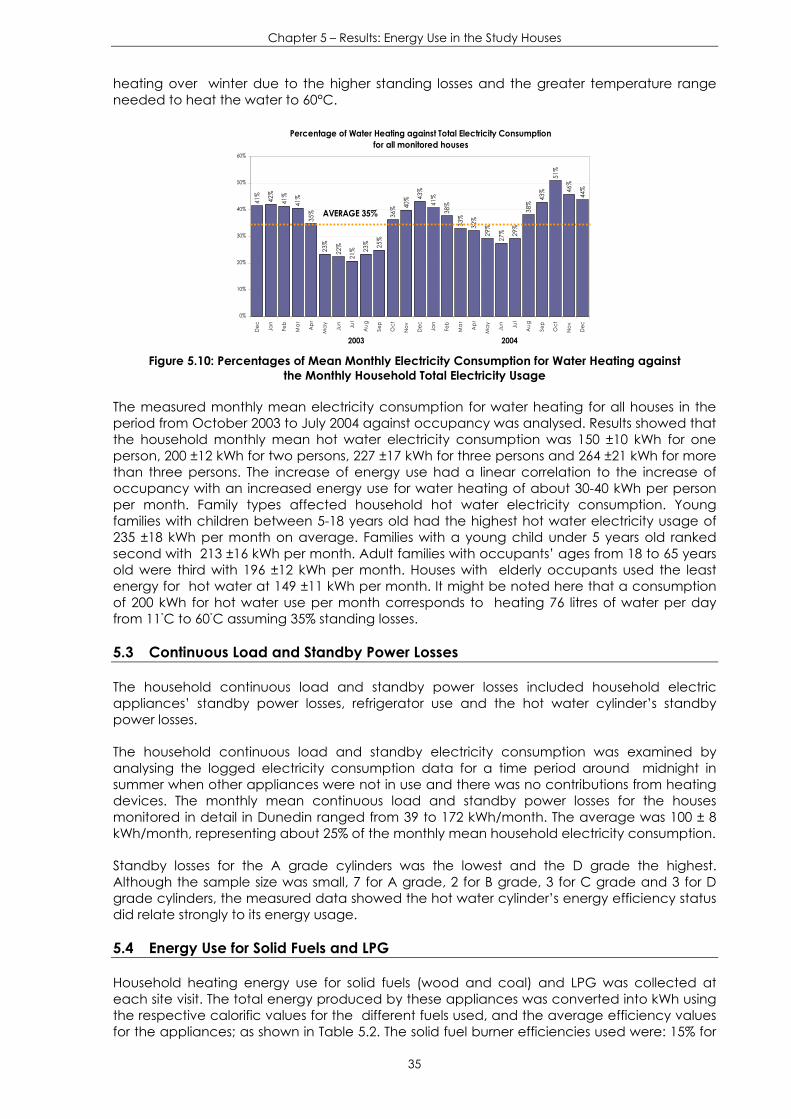
Chapter 5 – Results: Energy Use in the Study Houses
35
heating over winter due to the higher standing losses and the greater temperature range needed to heat the water to 60°C.
Percentage of Water Heating against Total Electricity Consumptionfor all monitored houses
41%
42%
41%
41%
35%
23%
22%
21% 23
% 25%
36% 40
% 43%
41%
38%
33%
32%
29%
27% 29
%
38%
43%
51%
46%
44%
0%
10%
20%
30%
40%
50%
60%
Dec Ja
n
Feb
Ma
r
Ap
r
Ma
y
Jun Jul
Aug
Sep
Oct
Nov Dec Ja
n
Feb
Ma
r
Ap
r
Ma
y
Jun Jul
Aug
Sep
Oct
Nov Dec
2003 2004
AVERAGE 35%
Figure 5.10: Percentages of Mean Monthly Electricity Consumption for Water Heating against the Monthly Household Total Electricity Usage
The measured monthly mean electricity consumption for water heating for all houses in the period from October 2003 to July 2004 against occupancy was analysed. Results showed that the household monthly mean hot water electricity consumption was 150 ±10 kWh for one person, 200 ±12 kWh for two persons, 227 ±17 kWh for three persons and 264 ±21 kWh for more than three persons. The increase of energy use had a linear correlation to the increase of occupancy with an increased energy use for water heating of about 30-40 kWh per person per month. Family types affected household hot water electricity consumption. Young families with children between 5-18 years old had the highest hot water electricity usage of 235 ±18 kWh per month on average. Families with a young child under 5 years old ranked second with 213 ±16 kWh per month. Adult families with occupants’ ages from 18 to 65 years old were third with 196 ±12 kWh per month. Houses with elderly occupants used the least energy for hot water at 149 ±11 kWh per month. It might be noted here that a consumption of 200 kWh for hot water use per month corresponds to heating 76 litres of water per day from 11˚C to 60˚C assuming 35% standing losses.
5.3 Continuous Load and Standby Power Losses
The household continuous load and standby power losses included household electric appliances’ standby power losses, refrigerator use and the hot water cylinder’s standby power losses.
The household continuous load and standby electricity consumption was examined by analysing the logged electricity consumption data for a time period around midnight in summer when other appliances were not in use and there was no contributions from heating devices. The monthly mean continuous load and standby power losses for the houses monitored in detail in Dunedin ranged from 39 to 172 kWh/month. The average was 100 ± 8 kWh/month, representing about 25% of the monthly mean household electricity consumption.
Standby losses for the A grade cylinders was the lowest and the D grade the highest. Although the sample size was small, 7 for A grade, 2 for B grade, 3 for C grade and 3 for D grade cylinders, the measured data showed the hot water cylinder’s energy efficiency status did relate strongly to its energy usage.
5.4 Energy Use for Solid Fuels and LPG
Household heating energy use for solid fuels (wood and coal) and LPG was collected at each site visit. The total energy produced by these appliances was converted into kWh using the respective calorific values for the different fuels used, and the average efficiency values for the appliances; as shown in Table 5.2. The solid fuel burner efficiencies used were: 15% for

Chapter 5 – Results: Energy Use in the Study Houses
36
open-fires and 60% for the multi-fuel burners (ECAN 2004). Un-ducted gas heaters were considered 100% efficient as all of the heat (and combustion products) stayed in the house.
Table 5.2 Calorific Values for Wood, Coal, and LPG (MED July 2003)
For the sample houses in Dunedin, the annual gross energy consumption from solid fuel and LPG use was estimated to be around 70-90% of the household yearly mean electricity usage, while the net heat input was about 30-45% of the annual mean household electricity usage. Houses with solid fuel and LPG for space heating used a daily average of around 6.5 kg of wood, 10.5 kg of coal and 0.55 kg of LPG for the month of July 2003.
The sample houses in Southland relied more on solid fuel and LPG for space heating. These houses used an average of about 6 kg of wood, 20 kg of coal and 0.65 kg of LPG per day for July 2003. Some individual houses used quite large quantities of coal in the inefficient open-fires.
5.5 Total Energy Use for houses in Samples A & B
The monthly mean energy consumption for electricity and other fuels usage (taking into account the burner efficiency factors for solid fuels, i.e. net use for solid fuels) for both samples (A and B) in Dunedin 2003/2004 is shown in Table 5.3. The percentage of each energy source is shown for all months as well as the progress of the upgrade for each sample.
Total energy consumption per annum is seen to be 8687kWh for both Samples with 22% for other fuels (1959 + 430 kWh) and 78% for Electricity (6728 + 180 kWh). The winter average (June to August) for electricity consumption is shown for comparison at the bottom of the table. These figures take into account the HDD differences for the period analysed allowing an estimate of the weather adjusted energy reduction. Table 5.4 shows total energy consumption for both samples for the years monitored with the estimated energy used for space heating.
Solid Fuel Calorific Values (Net): Wood (MJ/kg) Coal (MJ/kg) LPG (MJ/kg)
Fresh Wood 7.4 Ohai 23.69 60/40 45.65
Fuel Wood 10.3 KaiPoint 18.19 General 45.66
Container 13.3 Lignite 14.06 9 kg/Bottle
Furniture 16.3 NewVale 13.82 $1.72/kg
Oven-dried 19.2 Mataura 12.12 I kWh= 3.6 MJ
Density (kg/m3) Coal: 575, Fire Wood: 200-250
Burner Efficiency Factor Open fire: 15%, Multi-fuel burner: 60%
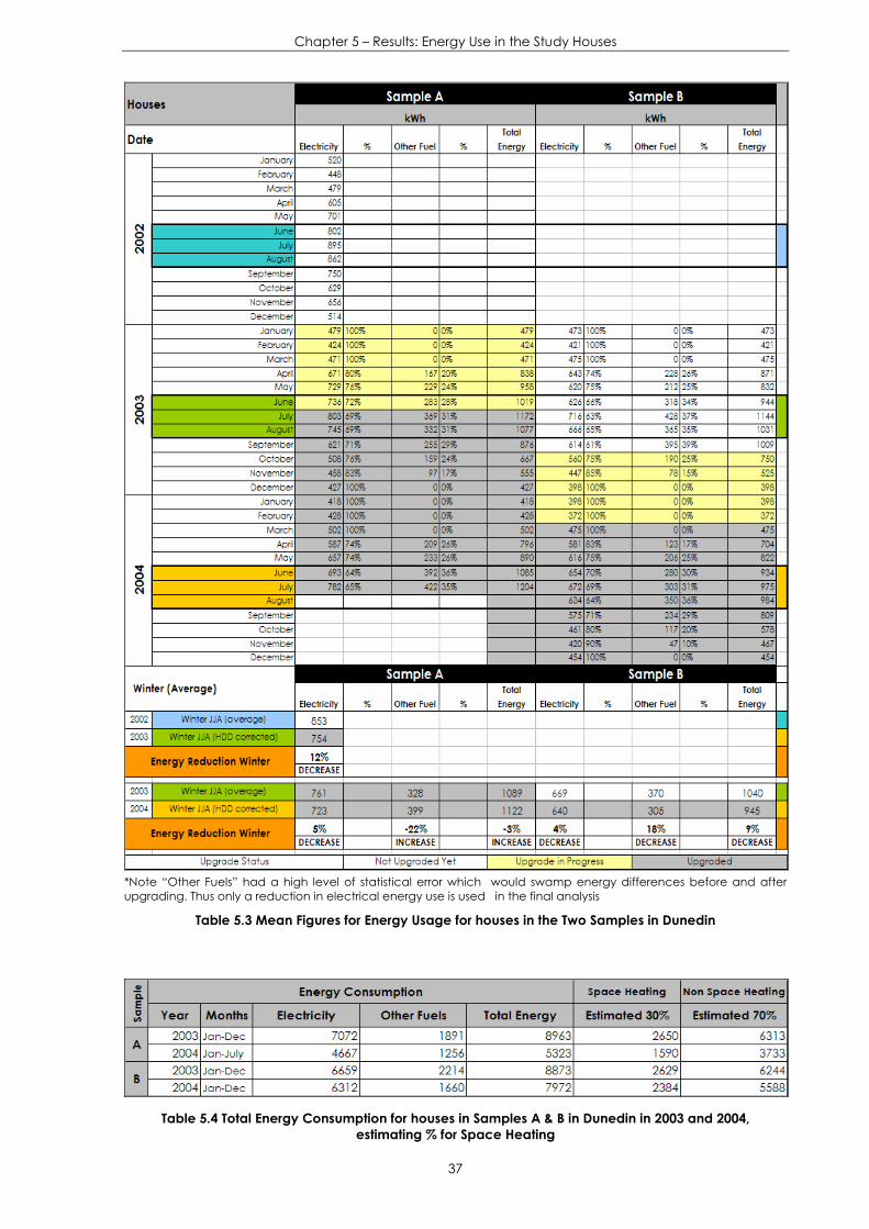
Chapter 5 – Results: Energy Use in the Study Houses
37
*Note “Other Fuels” had a high level of statistical error which would swamp energy differences before and after upgrading. Thus only a reduction in electrical energy use is used in the final analysis
Table 5.3 Mean Figures for Energy Usage for houses in the Two Samples in Dunedin
Table 5.4 Total Energy Consumption for houses in Samples A & B in Dunedin in 2003 and 2004, estimating % for Space Heating
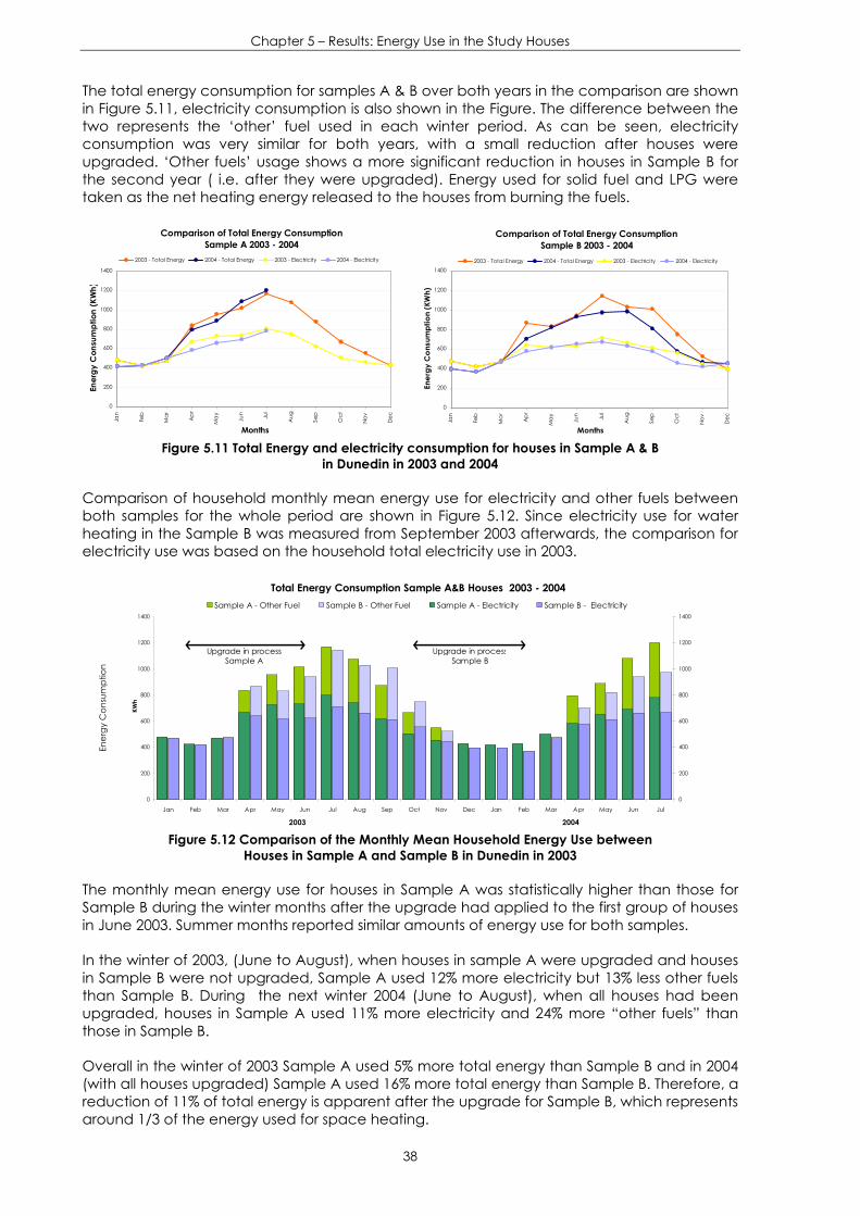
Chapter 5 – Results: Energy Use in the Study Houses
38
The total energy consumption for samples A & B over both years in the comparison are shown in Figure 5.11, electricity consumption is also shown in the Figure. The difference between the two represents the ‘other’ fuel used in each winter period. As can be seen, electricity consumption was very similar for both years, with a small reduction after houses were upgraded. ‘Other fuels’ usage shows a more significant reduction in houses in Sample B for the second year ( i.e. after they were upgraded). Energy used for solid fuel and LPG were taken as the net heating energy released to the houses from burning the fuels.
Comparison of Total Energy ConsumptionSample A 2003 - 2004
0
200
400
600
800
1000
1200
1400
Jan
Feb
Ma
r
Ap
r
Ma
y
Jun Jul
Aug
Sep
Oct
Nov Dec
Months
Ener
gy C
onsu
mpt
ion
(KW
h)
2003 - Total Energy 2004 - Total Energy 2003 - Electricity 2004 - Electricity
Comparison of Total Energy ConsumptionSample B 2003 - 2004
0
200
400
600
800
1000
1200
1400
Jan
Feb
Ma
r
Ap
r
Ma
y
Jun Jul
Aug
Sep
Oct
Nov Dec
MonthsEn
ergy
Con
sum
ptio
n (K
Wh)
2003 - Total Energy 2004 - Total Energy 2003 - Electricity 2004 - Electricity
Figure 5.11 Total Energy and electricity consumption for houses in Sample A & B
in Dunedin in 2003 and 2004
Comparison of household monthly mean energy use for electricity and other fuels between both samples for the whole period are shown in Figure 5.12. Since electricity use for water heating in the Sample B was measured from September 2003 afterwards, the comparison for electricity use was based on the household total electricity use in 2003.
Total Energy Consumption Sample A&B Houses 2003 - 2004
0
200
400
600
800
1000
1200
1400
Jan Feb Mar Apr May Jun Jul Aug Sep Oct Nov Dec Jan Feb Mar Apr May Jun Jul
2003 2004
KWh
0
200
400
600
800
1000
1200
1400
Sample A - Other Fuel Sample B - Other Fuel Sample A - Electricity Sample B - Electricity
Upgrade in processSample A
Upgrade in processSample B
Figure 5.12 Comparison of the Monthly Mean Household Energy Use between
Houses in Sample A and Sample B in Dunedin in 2003
The monthly mean energy use for houses in Sample A was statistically higher than those for Sample B during the winter months after the upgrade had applied to the first group of houses in June 2003. Summer months reported similar amounts of energy use for both samples.
In the winter of 2003, (June to August), when houses in sample A were upgraded and houses in Sample B were not upgraded, Sample A used 12% more electricity but 13% less other fuels than Sample B. During the next winter 2004 (June to August), when all houses had been upgraded, houses in Sample A used 11% more electricity and 24% more “other fuels” than those in Sample B.
Overall in the winter of 2003 Sample A used 5% more total energy than Sample B and in 2004 (with all houses upgraded) Sample A used 16% more total energy than Sample B. Therefore, a reduction of 11% of total energy is apparent after the upgrade for Sample B, which represents around 1/3 of the energy used for space heating.
Ener
gy C
onsu
mpt
ion

Chapter 5 – Results: Energy Use in the Study Houses
39
Houses in Sample A used more ‘other fuels’ for space heating during the second winter while houses in sample B presented a significant reduction in ‘other fuels’ after houses were upgraded. It is important to note that while houses in Sample A consumed more energy, they had slightly higher indoor temperatures. It also might be noted that Sample B had 5% more houses that used electricity for space heating as first choice, as compared with Sample A.
There was a similar monthly electricity consumption for water heating in the two housing samples in the summer and winter months. Houses in Sample B with a slightly lower occupancy used less electricity for non-hot water heating in each month. Houses in Sample A showed higher energy use for space heating than those in Sample B during winter 2004. The 16% more energy (electricity and fuels) spent by houses in Sample A from June to August was probably the reason why their indoor temperatures were slightly higher than those in Sample B houses in the winter of 2004 (see chapter 4).
5.6 Comparison of Energy Use for the Same Sample of Houses in 2003 and 2004 (with different weather conditions and same occupants)
This section compares energy consumption taking into account the difference in weather conditions and also the status of upgrade (i.e. non upgrade houses are being compared with the same houses after being upgraded the following winter).
As it can be seen in Table 5.5 there were higher HDD for year 2004 compared with the year before in most of the months, suggesting more energy would be needed for space heating for the second winter in the comparison. The difference between both years is shown at the bottom of the table. By taking into account HDD differences for both years it can be calculated how much energy it would be expected to be used to achieve the same temperature in the following year if the same physical conditions applied. As differences in indoor temperatures were known, any difference recorded in energy use could be attributed to a change in physical aspects of the house (eg insulation), change in occupants behaviour and/or any other weather conditions as wind and isolation variations.
HDD Year Jan Feb Mar Apr May Jun Jul Aug Sep Oct Nov Dec
2003 108 109 122 219 258 284 360 335 276 251 198 134
2004 71 137 164 237 269 306 367 372 283 248 167 231 dif 37 -28 -42 -18 -11 -22 -7 -38 -7 3 31 -96
Table 5.5 Heating Degree Days for 2003 & 2004
Sample A
A comparison of the household monthly mean energy use for electricity and other fuels for the Sample A houses in 2003 and 2004 is shown in Figure 5.13. Energy use for water heating remained the same in the same months before and after the insulation upgrade because few hot water cylinders had been insulated.
0100200300400500600700800900
10001100120013001400
Jan
Feb Mar Apr May Jun Ju
l
kWh
Fuel 2004Non-Hot Water 2004Hot Water 2004Fuel 2003Non-Hot Water 2003Hot Water 2003
Figure 5.13 Comparison of the Monthly Mean Household Energy Use and Hot Water
for Houses in Sample A in 2003 and 2004
Ener
gy C
onsu
mpt
ion
(kW
h)

Chapter 5 – Results: Energy Use in the Study Houses
40
The historical electricity consumption for the period before the upgrade (July 2002 to June 2003) was compared with the monitored electricity consumption after the upgrade (July 2003 to June 2004). The corrected reduction was found to be between 11% and 15% for electricity only.
Sample A houses had a reduced electricity consumption during winter months of 12% after the upgrade (2002 vs. 2003) and had had a further reduction of 5% when comparing both winters with all houses upgraded (2003 vs. 2004). With the colder weather in 2004, there was about 22% more ‘other fuels’ used for space heating in that year. There was a similar amount of energy used in July over the two years under the same weather conditions and with all houses being upgraded.
Sample B
A comparison of household monthly mean energy use for electricity and other fuels for houses in Sample B in 2003 and 2004 is shown in Figure 5.14. In this case, houses were upgraded during the summer months while being monitored, allowing comparison over both winters before and after insulation. This sample of houses showed a small reduction in electricity use for non-hot water energy when comparing both years, but a higher reduction was found in ‘other fuels’ used for space heating (data collected for water heating was available from October 2003 onwards). A comparison can be made for both years by estimating similar hot water usage assuming similar behaviour from the occupants for both years.
Total Energy Consumption Sample B Houses 2003 - 2004
0
200
400
600
800
1000
1200
1400
Jan Feb March April May June July Aug Sep Oct Nov Dec
Months
KWh
0
200
400
600
800
1000
1200
1400
2003 Other Fuel 2004 Other Fuel 2003 Electricity 2004 Electricity Total Electricity Consumption Sample B Houses 2003 - 2004
0
200
400
600
800
1000
1200
1400
Jan Feb March April May June July Aug Sep Oct Nov Dec
Months
KWh
0
200
400
600
800
1000
1200
1400
2003 Non Hot Water 2004 Non Hot Water 2003 Hot Water 2004 Hot Water
Figure 5.14 Comparison of the Monthly Mean Household Energy Use and Hot Water for houses in Sample
B in 2003 and 2004
For the whole year analysis, in 2004, houses in Sample B used 7% less electricity and 26% less ‘other fuels’ than in 2003. As it can be seen the difference in energy consumption for this sample of houses was mainly due to the large reduction of ‘other fuels’ energy use for space heating on during the second year. Note: As mentioned previously, the statistical errors in the ‘other fuels’ energy use make any conclusions regarding this data statistically insignificant.
During the winter months (June-August) after the upgrade, the total household energy consumption for Sample B showed a reduction of about 9%, based on comparing data for the winter 2003 (non upgraded) against the winter of 2004 (upgraded) for electricity and other fuels. In the winter of 2004, after houses were upgraded, Sample B used 4% less electricity and 18% less other fuels than in 2003. While Sample B showed a decrease in electricity consumption for space heating, it also showed an increased net indoor temperature difference in winter of 0.6°C.
Summary
The annual mean household total energy use for all houses in Dunedin was 8687 kWh which was composed of 6728 kWh + 181 kWh (78%) for electricity consumption and 1959 kWh + 430kWh (22%) for other fuels.
After correction of the space heating energy usage for weather conditions, a reduction of between 7% and 13% in electricity consumption was recorded after the upgrade for Dunedin
Ener
gy C
onsu
mpt
ion
(kW
h)

Chapter 5 – Results: Energy Use in the Study Houses
41
houses participating in this research. This reduction represents between 5% and 9% of the total household energy use. The weather corrected decrease in ‘other fuels’ was -16% (ie. an increase) for Sample A and +34% for Sample B comparing 2003 with 2004 but with a standard deviation in the mean consumption of ‘other fuels’ of 22% neither change could be considered significant.
Comparison for the winter months only from June to August after houses were upgraded showed a reduction of between 4% and 12% for electricity only. This reduction in electricity consumption during winter would have an impact of between 3% and 9% on the total winter energy consumption. This represents between 1/6 and 1/3 of the energy used for space heating. In addition to the decrease in energy consumption the sample houses also exhibited a net indoor temperature improvement over the winter months of 0.6 + 0.2˚C.
The annual reduction in electricity consumption found in Dunedin houses after the upgrade was between 5% and 9% of the total household energy consumption. As energy consumption for space heating accounts for around 30% of the total annual consumption (Isaac, N. et at 2004), we can estimate that the reduction represents between 1/6 and 1/3 of energy consumption used for space heating. Houses also increased their annual indoor temperature by 0.4 + 0.2˚C.

Chapter 6 – Intensive monitoring of two State Houses in Dunedin
42
Intensive monitoring of two State Houses in Dunedin Chapter 6
As the efficacy of the HNZC upgrade program was not obvious from the main monitoring program, two State Houses participating in the energy efficient upgrade program located in Dunedin were selected to be intensively monitored over a short time period. The aim was to identify specific improvements in the thermal performance of the building envelope after both houses were upgraded. A brick veneer house and a weatherboard house were each intensively monitored over a two weeks period, with no occupants and on loan from HNZC. The monitoring recorded changes in indoor temperatures and energy input as well as ambient weather conditions. Data collected was then used for simulation in both steady state and dynamic modelling tools (ALF3 and Virtual Environment). Model results were then validated against the monitored performance of the houses.
6.1 Methodology
The houses were first investigated using a lumped thermal resistance model, looking at losses and gains from applied heating but with no solar gains. The houses were heated with electric resistance heating, during times when the ambient temperature was reasonably constant and there was no solar gain to a steady state internal temperature. Air circulation fans were used to reduce temperature stratification and differences in the rooms as much as possible. Measured indoor temperatures taken during these times were compared with the model. Houses were then modelled using ALF3 and Virtual Environment and results were compared with the measurements.
Once the VE model was tuned to give good agreement between actual measurements and the simulated results over short time periods, the software was used to model a typical Housing NZ house (both before and after the upgrade) over the years 2003 and 2004. The model results were then compared with the actual monitoring data.
Steady State Analysis
The specific thermal losses in W K-1 were determined through the total envelope of the building. Data were collected from the houses to be able to make this analysis before and after the upgrade allowing an estimation to be made for the difference in the lumped thermal resistance of the building envelope.
Monitoring Process
Temperatures Monitoring:
In order to monitor the variation in indoor temperature, iButton data loggers were placed in each room. The loggers were set to record at 3 minute intervals at two different heights (1 m and 2 m) for the whole monitoring period for each room in both houses.
Ambient temperatures were obtained from a calibrated weather station at the Physics Department (University of Otago) which was 2.4 km from the monitoring site. In addition, iButtons were also installed outside of the houses under the eaves but as these measurements were affected by heat gains from the internally heated houses, they were not used for heat loss calculations.
Energy input:
Constant power output electric resistance heaters were installed at a power level close to 2 kW per 13.4 m2 of floor space (around one 2 kW heater per room). The heaters were calibrated before and after the monitoring process using a digital watt meter (Topward - Aameter 1301). A circulation fan was installed to generate internal air movement and to minimize the stack effect of warm air rising to the ceiling. Electricity consumption was

Chapter 6 – Intensive monitoring of two State Houses in Dunedin
43
recorded by on site meter reading. External windows were checked to be all closed during the monitoring period.
House 1 was monitored during one week before and one week after the house was upgraded (with the standard HNZC upgrade package) with 5 heaters providing a constant thermal power of around 10 kW (2kW each heater). All internal doors in the house were left open during the tests and the fan provided additional forced circulation.
In the case of House 2, the analysis concentrated on measurements in the living room and bedroom 2. The thermal performance was examined before and after the upgrade. In this case the ‘after upgrade’ analysis had a second stage whereby additional upgrade work was undertaken to improve the thermal performance. This additional work included detailed sealing of the building envelope (reducing air leakage by around 40%) and the installation of thick curtains. Whereas the heaters in House 1 were manually controlled, the heaters in House 2 had on-off timers installed to automatically turn them on at 4:20 pm and off at 8:00 am (i.e. at times with no solar gain during winter months) .
Air Tightness:
A standard blower door test was used to quantify the amount of air leakage in both houses, before and after upgrade.
Modelling
Two simulation programs were used for further modelling the houses: ALF and VE.
The ALF (Annual Loss Factor) method was developed by BRANZ for NZ use only and is a steady state model of heat gain and loss. It uses historical local climate information and has four different heating schedules, at three different temperatures (16ºC, 18ºC and 20ºC). The house physical dimensions collected from site survey were entered into the program together with information on the construction materials of the houses in order to simulate the thermal performance.
Virtual Environment is a dynamic model created by IES in the UK. It is a complete building-
modelling package including dynamic thermal simulation. Physical data from the house was entered into the program together with actual local weather from the Physics weather station and actual heating schedules.
6.2 The two houses…
Figure 6.1 Aerial photo of both houses (18, Dover St. & 22, Forrester St. Pine Hill, Dunedin)
Both State Houses were located in the Pine Hill suburb of Dunedin (see aerial photos figure 6.1). Details for each house are provided in Table 2 and in the following notes.
House 1 was a two bedroom weatherboard house; built in the 1950s. Layout is shown in Figure 6.2. The house was a single story house, surrounded by garden with good solar access. The home had a suspended floor, which was elevated 1.2 m from the ground and enclosed by a brick wall. In this case the upgrade involved the total HNZC energy
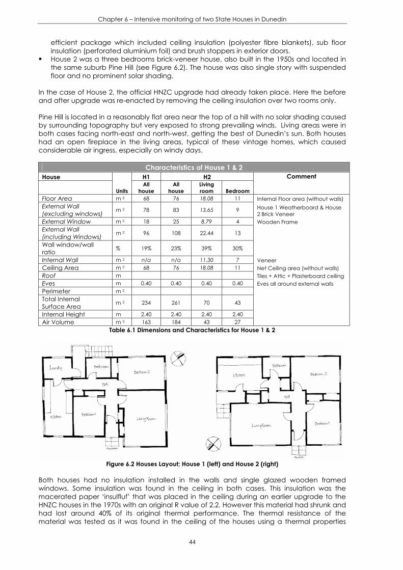
Chapter 6 – Intensive monitoring of two State Houses in Dunedin
44
efficient package which included ceiling insulation (polyester fibre blankets), sub floor insulation (perforated aluminium foil) and brush stoppers in exterior doors.
House 2 was a three bedrooms brick-veneer house, also built in the 1950s and located in the same suburb Pine Hill (see Figure 6.2). The house was also single story with suspended floor and no prominent solar shading.
In the case of House 2, the official HNZC upgrade had already taken place. Here the before and after upgrade was re-enacted by removing the ceiling insulation over two rooms only.
Pine Hill is located in a reasonably flat area near the top of a hill with no solar shading caused by surrounding topography but very exposed to strong prevailing winds. Living areas were in both cases facing north-east and north-west, getting the best of Dunedin’s sun. Both houses had an open fireplace in the living areas, typical of these vintage homes, which caused considerable air ingress, especially on windy days.
Characteristics of House 1 & 2 House H1 H2
Units All
house All
house Living room Bedroom
Comment
Floor Area m 2 68 76 18.08 11 Internal Floor area (without walls) External Wall (excluding windows) m 2 78 83 13.65 9 House 1 Weatherboard & House
2 Brick Veneer External Window m 2 18 25 8.79 4 Wooden Frame External Wall (including Windows) m 2 96 108 22.44 13
Wall window/wall ratio % 19% 23% 39% 30%
Internal Wall m 2 n/a n/a 11.30 7 Veneer Ceiling Area m 2 68 76 18.08 11 Net Ceiling area (without walls) Roof m Tiles + Attic + Plasterboard ceiling Eves m 0.40 0.40 0.40 0.40 Eves all around external walls Perimeter m 2 Total Internal Surface Area m 2 234 261 70 43
Internal Height m 2.40 2.40 2.40 2.40 Air Volume m 3 163 184 43 27
Table 6.1 Dimensions and Characteristics for House 1 & 2
Figure 6.2 Houses Layout; House 1 (left) and House 2 (right)
Both houses had no insulation installed in the walls and single glazed wooden framed windows. Some insulation was found in the ceiling in both cases. This insulation was the macerated paper ‘insulfluf’ that was placed in the ceiling during an earlier upgrade to the HNZC houses in the 1970s with an original R value of 2.2. However this material had shrunk and had lost around 40% of its original thermal performance. The thermal resistance of the material was tested as it was found in the ceiling of the houses using a thermal properties

Chapter 6 – Intensive monitoring of two State Houses in Dunedin
45
analyser (QL-30, Anter Corp – US) to have an R value of 1.32 K m2 W-1 for a 60mm thickness. It would be expected that considerable variation in this value would occur as the surface was observed to be quite uneven.
6.3 Results: Modelling the theory
Thermal modelling was accomplished using R values incorporating standard thermal resistances of the materials and structures these values were obtained from “Energy Efficient Building Design” (Hoger, W. 2000) and “Introduction to Architectural Science”(Szokolay, S.V. 2004). R-Values used are given in Table 6.2.
Characteristics of materials - House 1 & 2
Components R-Value U-value K m2 W-1 W K-1 m-2
Tiled roof - With original insulation 1.7 0.59 Tiles 0.3
Insulfluf 1.32 Plasterboard 0.08
Tiled roof - With new insulation 4.7 0.21
Roof
Polyester Blankets 3 Timber stood frame – No insulation 0.7 1.43
Weatherboard 0.62 Air gap 0
Wa
ll H1
Plasterboard 0.08 Brick Veneer - No insulation 0.56 1.79
Brick 0.46 Air gap 0
Wa
ll H2
Timber Frame + Plasterboard 0.1 Timber floor with carpet - No insulation 0.9 1.1
Timber + floor joists + bearers + piers 0.6 Carpet 0.3
Timber floor with carpet and foil insulation 1.2 0.83 Floo
r
Foil Insulation 0.3 Basement Wall - Continuous Glass 0.16 6.25
Oth
ers
Glass and Thermal Curtains 0.21 4.76
Measured original ACH H1 - all 1.1 H2 - all 1.2
H2 – Living 1.1 Air
Inf
H2 – Bedroom 1.2 Table 6.2 Thermal Resistances of Materials showing R-values & U-values for House 1 & 2
The specific thermal losses through each component of the building envelope, for House 1, were calculated before and after the upgrade (Table 6.3). As can be seen, the steady state modelling suggests an expected 0.07 K m2 W-1 increase in the lumped thermal resistance R-value after the upgrade.
U value R value W K-1 House 1 Area Before After Before After Before After Floor 68 1.10 0.83 0.91 1.20 75 56 Walls 79 1.43 1.43 0.70 0.70 113 113
Windows 18 6.25 6.25 0.16 0.16 113 113 Ceiling 68 0.59 0.21 1.69 4.76 40 14
Air Infiltration 62 62 H1 -
TEST
1 &
2
Total Surface 233 402 358
R-va
lue
Impr
ovem
ent
0.07 R-value (K m2 W-1) 0.58 0.65 12% Table 6.3 Improvement in lumped thermal resistance House 1 – Before & After the Upgrade (Test 1&2)
The same analysis was repeated for house 2 which showed an improvement of between 0.05-0.06 K M2 W-1 for the living room and bedroom 2 after the standard HNZC upgrade. With the additional upgrade work, a final improvement of 0.07 K m2 W-1 for the living room after

Chapter 6 – Intensive monitoring of two State Houses in Dunedin
46
reducing air leakage and a final R value improvement of 0.15 K m2 W-1 in the bedroom after reducing heat losses through the single glassed windows by providing thick curtains was calculated.
6.4 Results: Physical monitoring of the houses
Results for House 1:
Test-1 was undertaken by monitoring the house during three days before the upgrade. The house was then upgraded on the fourth day. Testing resumed on the upgraded house as Test 2 which was undertaken during the next consecutive three days.
The whole house was heated during all the tests, external windows were closed, the fireplace was sealed and all internal doors were left open. The significant level of heating applied meant that large temperature differences could be induced thus reducing percentage errors. The mean indoor temperature was calculated by averaging the outputs of all indoor temperature data loggers. The net temperature differences (defined as the differences between the indoor and ambient temperatures) were then found using the measured ambient temperatures obtained from the Physics department weather station. The equilibrium temperature values were obtained overnight between 1:00AM and 5:00AM thus avoiding any solar gain and at times when ambient was reasonably steady.
Test 1: 3 days before the upgrade: all house net temperature difference = 18.7ºC Test 2: 3 days after the upgrade: all house net temperature difference = 19.5ºC
Results thus showed an increase in net temperature difference (NTD) of about 0.8ºC after the upgrade. Considering that Q = Area of Surface x ∆t / U, results show that:
Before the upgrade: U value 2.00 W K-1 m-2 which equals to R-value of 0.5 K m2 W-1 After the upgrade: U value 1.88 W K-1 m-2 which equals to R-value of 0.54 K m2 W-1
As it can be seen only a small difference in the total resistance of the building envelope was detected after the upgrade. The R value improves by only by 0.04 K m2W-1 (8%) compared to the value of 0.07 Km2W-1 or 12% improvement calculated using the steady state lumped resistance model.
Results for House 2:
House 2 was tested by monitoring the house three days before being upgraded (test 1 with the insulation withdrawn from bedroom 2 and the living room). The after upgrade monitoring (all insulation in place) was accomplished over two days for the standard upgrade only (test 2), then a further two days with the additional upgrade consisting of sealing the living room (test 3) and a final 2 days during which curtains were installed in the bedroom (test 4).
The living room and bedroom were heated from 4:00PM to 8:00AM, the external windows and doors were closed and fire place was sealed. Indoor temperature was increased achieving steady state in the early morning as before. Data collected was used to calculate net differences. Again, the equilibrium values were calculated between 1:00AM and 5:00AM, to avoid any solar heating. Houses recorded net temperature differences for each test of:
Test 1: 3 days before the upgrade: living room NTD = 20.6ºC & bedroom NTD = 21.8ºC Test 2: 2 days after the upgrade: living room NTD = 20.9ºC & bedroom NTD = 22.5ºC Test 3: 2 days after the upgrade & sealing: living room NTD = 21.7ºC Test 4: 2 days after the upgrade & curtains: bedroom NTD = 26.0ºC
Results show an increase in net temperature differences after the upgrade. Thus after the upgrade the building envelope has increased its R value. Results are shown for each test:

Chapter 6 – Intensive monitoring of two State Houses in Dunedin
47
Test 2 (Average of Days 4 to 6). After upgrading the house with the standard energy efficiency package, the results show a net temperature difference improvement of 0.3ºC for the living room and 0.7ºC for the bedroom after the upgrade. The corresponding R values showed an increase of around 0.03 K m2 W-1.
Test 3 (Average of Days 6 to 8). After upgrading the house and reducing around 40% of total air leakage by sealing the living room, results have showed a NTD increase of 1.1ºC. The corresponding R values shows an increase of 0.04 K m2 W-1
Test 4 (Average of Days 6 to 8). After upgrading the house and reducing heat losses through the windows by installing curtains in the bedroom, which might have some impact in reducing some air leakage, results have shown a net temperature difference improvement of 4.2ºC. The corresponding increase in R values is 0.1 K m2 W-1
Similar to the results for the first house, House 2 demonstrated a low increase in R value, for the two rooms only, after upgrading of 0.03 K m2 W-1. Improving the sealing in the living room by around 40% gave an increase in the R value for this room of about 0.04 K m2 W-1. Finally, reducing heat losses through windows by using thick curtains gave a higher increase of 0.1 K m2 W-1 in the R value for the bedroom suggesting that this may be a useful way to improve the R value of the houses.
Summary
Figure 6.2 shows the modelling of heat losses through different components of the building envelope for House 1. The first house figure gives an estimate of how the building performed as originally built in the 1950s with no insulation anywhere. The second figure shows the house as found before the 2004 upgrade with the ‘insulfluf’ insulation in place that was installed in the ceiling in the 1970’s retrofit. The third house figure shows the house after upgraded by the latest HNZC energy efficiency program.
As it can be seen there is only a small percentage improvement likely to be attributed to the new insulation installed in the ceiling during the last upgrade. Only 4% of the final heat losses occur through the insulated ceiling. The first insulation upgrade using the “insulfluf” was providing reasonable heat retention even though the material had shrunk and had lost some of its original thermal characteristics. This material had reduced the heat losses through the ceiling from 32% for the original un-insulated ceiling to just 10%. Adding more insulation on the top of the insulfluf would reduce the losses occurring through the ceiling by only 6% (with total losses for the double insulated ceiling being only 4% of the total losses).
House Original House ‘70s Retrofit House Upgraded 2005
538 W K-1 402 W K-1 357 W K-1 25% reduction 11% reduction
Figure 6.3 House 1: % of Heat Losses through the different components of the building envelope
As little had been done to the rest of the building envelope and not much to the air tightness of the houses, the single glazed windows accounted for 31% and the un-insulated walls accounted for 32% of total losses. The upgraded floor and air infiltration represent around 17% total losses each.
4%
32%
16%
31%
17%
10%
28%
19%
28%
15%
32%
21%
14%
21%
12%

Chapter 6 – Intensive monitoring of two State Houses in Dunedin
48
Figure 6.3 shows similar results for House 2. A higher reduction (21%) of heat losses through the ceiling was found after the first 1970s upgrade. Again the new upgrade had only reduced a further 5% of the losses through the insulated ceiling. Walls and windows accounted for more than 60% of the losses and air infiltration and floor accounted for around 15%.
House Original House ‘70s Retrofit House Upgraded 2005
663 W K-1 509 W K-1 459 W K-1 23% reduction 10% reduction
Figure 6.4 House 2: % of Heat Losses through the different components of the building envelope
As it can be seen only a small reduction in the original thermal losses through the ceiling were achieved by installing the new insulation as in the current HNZC upgrade. This small decrease in heat losses then is the main reason why there was so little improvement in terms of improved indoor temperatures in both these intensively monitored homes and in the upgraded homes reported in the main test results.
HOUSE 1
0
50
100
150
200
250
Ceiling Floor Walls Windows Air Infiltration
W/˚
C
non insulated (original) 70s upgrade 2004 upgrade
HOUSE 2
0
50
100
150
200
250
Ceiling Floor Walls Windows Air Infiltration
W/˚
C
non insulated (original) 70s upgrade 2004 upgrade
Figure 6.5 Comparison of heat losses through the different components of the building envelope:
original vs. ’70s retrofit vs. 2004 upgrade package (House 1 & 2)
4%
32%
14%
34%
16%
9%
29%
17%
30%
15%
30%
22%
13%
24%
11%

Chapter 6 – Intensive monitoring of two State Houses in Dunedin
49
6.5 Results: Modelling with Virtual Environment
While ALF3 gives the steady state results the time dependant situation needs a dynamic simulation package such as that provided by Virtual Environment. To this end both houses were modelled using this package where the weather data to the model was provided by the actual weather measurements obtained from the Physics Department weather station. House 1 was modelled by Virtual Environment and the results for bedroom 2 (facing south) are shown in Figure 6.6. The first graph shows the monitoring period before the upgrade and the second graph shows the period after the upgrade. The thick line represents our measurements on site and the dotted line provides the VE simulation. As it can be seen, the VE model results are in remarkable agreement with the results recorded by our instrumentation. The cooling rate occurs faster some days in the model, which suggests that there might be some lower value in the thermal mass assumed by the program for this weatherboard house.
House 1 - Before Upgrade
0.00
5.00
10.00
15.00
20.00
25.00
30.00
35.00
40.00
45.00
0.0 12.0 24.0 36.0 48.0 60.0 72.0 84.0 96.0 108.0 120.0 132.0 144.0
Tem
p ºC
VE - BED BED -MONITORED AMBIENT
House 1 - After Upgrade
0.00
5.00
10.00
15.00
20.00
25.00
30.00
35.00
40.00
45.00
180.0 192.0 204.0 216.0 228.0 240.0 252.0 264.0 276.0
Tem
p ºC
VE - BED AMBIENT BED MONITORED
Figure 6.6 House 1: Thermal performance of Bedroom 2 - VE vs. measured
before and after the upgrade
House 2 was also modelled by Virtual Environment and the results for the living room are shown in Figure 6.7. The first graph shows the monitored days before the upgrade and the second graph shows results after the upgrade. As before the thick line represents our measurement and the dotted line is gives the VE simulation predicted values. As it can be seen the agreement is again good but not quite as good as for house 1. Again there is some suggestion that problems with the thermal mass of the brick house may account for the differences.

Chapter 6 – Intensive monitoring of two State Houses in Dunedin
50
House 2 - Before upgraded - Test 1
0.00
5.00
10.00
15.00
20.00
25.00
30.00
35.00
40.00
36 48 60 72 84 96 108
Tem
p ˚C
VE Bedroom Ambient Bedroom UP Ambient
Day 1 Day 2 Day 3 Day 4Day 1 Day 2 Day 3 Day 4
House 2 - After Upgrade - Test 2-3-4
0
5
10
15
20
25
30
35
40
12 24 36 48 60 72 84 96 108
Tem
p ºC
VE Bedroom Ambient Bedroom Monitored
Day 4 Day 5 Day 6 Day Figure 6.7 House 2: Thermal performance of bedroom - VE vs. measured
before and after the upgrade
House 2 - Before upgraded - Test 1
0
5
10
15
20
25
30
35
36 48 60 72 84 96 108
Tem
p ˚C
VE Livingroom Ambient LIVING 1
Day Day 2 Day 3 Day 4
House 2 - After Upgrade - Test 2-3-4
0
5
10
15
20
25
30
35
40
12 24 36 48 60 72 84 96 108
Tem
p ºC
VE Livingroom Ambient Livingroom - Monitored
Day 4 Day 5 Day 6 Day Figure 6.8 House 2: Thermal performance of livingroom - VE vs. measured
before and after the upgrade
Test 1: Day 1 to 4 (Before the upgrade) Test 2: Day 4 to 6 (Upgraded with the Energy Efficient Package) Test 3: Day 6 to 8 (Living room sealing: reducing air leakage) Test 4: Day 6 to 8 (Bedroom with curtains)

Chapter 6 – Intensive monitoring of two State Houses in Dunedin
51
24 HOUR PROFILE - HOUSE 2 - VE
0.0
2.0
4.0
6.0
8.0
10.0
12.0
14.0
16.0
18.0
20.0
0.0 6.0 12.0 18.0 24.0
HOURS
TEM
PERA
TURE
˚C
Bedroom before Upg Liv ing before Upg Bedroom after Upg Liv ing after Upg Ambient
Figure 6.9 House 2: 24 Hour profile
In addition, a 24 hour temperature profile was investigated for House 2 under more normal heating conditions. The situation was simulated by providing 1.5 kWh of constant heating applied to the living area from 5 pm to 10 pm during a winter month. The aim of the simulation was to compare the thermal performance of the building to real data. The simulation (see Figure 6.9) shows that the building would achieve higher temperatures after the upgrade when heating is applied to the living room, and in addition it shows that the room cools down slower overnight. This result is in good agreement with the data measurements in the real houses (see chapter 4) suggesting, however, that some of the benefit of the upgrade would occur after the occupants leave the heated room overnight. It should be noted that other internal gains were not added to the model in this simulation. In addition, the measurements presented in chapter 4 are the averages of all the houses in the Dunedin sample thereby smoothing the data considerably. Overall net temperature, differences however, are similar to those measured, with higher values observed during sleep hours, (see the 24 hour profile analysed in chapter 5).
6.6 Computer Modelling vs. Real Data: Samples A & B in Dunedin
Modelling with Virtual Environment Once the dynamic behaviour of the VE model was considered to be consistent with measured data, House 2 was simulated with different levels of space heating energy, with the aim to compare changes after the upgrade in condition similar to those found in practice. The modelling results can be seen in figure 6.10. Here temperature increases are plotted as a function of the space heating energy before and after the upgrade. The simulations were undertaken both for the whole year and for winter months (June to August) and results were compared with measured data for Sample A and B in Dunedin. The simulation output was found to be consistent with our measurements, in particular that the simulations predict: A temperature increase of 0.5ºC in the annual average temperatures of the living area
after the upgrade if the same energy is applied before and after the upgrade (2,700 kWh per annum). If the temperature is forced to remain constant after the upgrade a reduction of 20% in annual energy consumption for space heating is achieved after the upgrade (at 14.7ºC annual average temperature).
A temperature increase of 0.84ºC in the average temperature over the winter months of June to August if the same energy is applied before and after the upgrade (at 1600kWh per three months). If the temperature is forced to remain constant after the upgrade a reduction of 18% in winter energy consumption for space heating is achieved after the upgrade (at 13.2ºC average temperature over the three months of June – August).
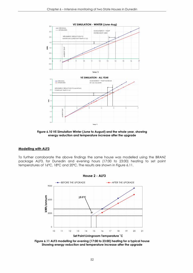
Chapter 6 – Intensive monitoring of two State Houses in Dunedin
52
VE SIMULATION - WINTER (June-Aug)
-1.0
-0.5
0.0
0.5
1.0
1.5
2.0
2.5
3.0
6 7 8 9 10 11 12 13 14 15 16 17
Temp ˚C
MW
h
ORIGINALUPGRADED SAME ENERGY = TEMP
INCREASE BY 0.85C @ 6 h
18% ENERGY REDUCTION TO MAINTAIN CONSTANT TEMP @ 13.2
AM
BIEN
T TE
MP
VE SIMULATION - ALL YEAR
-3.0
-2.0
-1.0
0.0
1.0
2.0
3.0
4.0
5.0
10 11 12 13 14 15 16 17
Temp ˚C
MW
h
ORIGINALUPGRADED
20% ENERGY REDUCTION TO MAINTAIN CONSTANT TEMP @ 14.7
SAME ENERGY = TEMP INCREASE BY 0.5C @2.5MWh
AM
BIEN
T TEM
P
Figure 6.10 VE Simulation Winter (June to August) and the whole year, showing energy reduction and temperature increase after the upgrade
Modelling with ALF3 To further corroborate the above findings the same house was modelled using the BRANZ package ALF3, for Dunedin and evening hours (17:00 to 23:00) heating to set point temperatures of 16ºC, 18ºC and 20ºC. The results are shown in Figure 6.11.
House 2 - ALF3
0
3000
6000
9000
10 11 12 13 14 15 16 17 18 19 20 21
Set Point Livingroom Temperature ˚C
kWh/
annu
m
BEFORE THE UPGRADE AFTER THE UPGRADE
+0.5°C
Figure 6.11 ALF3 modelling for evening (17:00 to 23:00) heating for a typical house
Showing energy reduction and temperature increase after the upgrade

Chapter 6 – Intensive monitoring of two State Houses in Dunedin
53
By interpolating the whole house set point temperatures, an increase of 0.5ºC in whole house temperature is predicted by ALF3 after the upgrade at a heating level of 2700kWh/annum (which was the average amount of energy applied for space heating for State houses in Dunedin participating in the program). This result is again consistent with our measurements. In addition ALF3 gives an annual energy saving of about 19% if the house set point indoor temperatures are not allowed to increase after the upgrade (i.e. at 16ºC).
These results using ALF3 are probably somewhat fortuitous, however, as it is known that “ALF3 reliability will decrease with internal temperatures below 14ºC as the temperature difference between inside and outside is too small, and above 22ºC as the supporting modelling did not explore these temperatures” (Isaacs N., 2005). In addition, the ALF3 temperatures are whole house temperatures and the heating regimes are for the whole house.
Comparing modelling with measurements… The modelling results (see figure 6.12 and Table 6.4) for indoor temperature increases and space heating energy reductions after the upgrade are consistent with the measurements taken in the sample houses participating in the research (green rectangle). For the whole year both programs (VE and ALF3) have suggested that with a constant space heating level of 2700 kWh/annum (corresponding to about the levels observed in the HNZC sample) a temperature increase of 0.5ºC (annual average) is observed after the upgrade. Our measurements have shown an increase of between 0.2 - 0.6ºC in annual average indoor temperature, with a reduction of between 5 - 9% of electricity consumption (16 - 30% of energy for space heating). The graphs below also show the situation for houses with electric heating only (pink), which also show a slightly higher indoor temperature increase and similar energy consumption after the upgrade.
Figure 6.12 Space heating energy reduction: VE Modelling against Measurements
Winter and all year
Temperature Increase ºC Space heating energy decrease %
with space heating energy
decrease
with constant space heating
energy
with constant indoor
temperature
with 0.2ºC increase in
indoor temp. all year
with 0.5ºC increase in
indoor temp. winter
Measurements Full year 0.2 - 0.6 - - 15 - 30% - VE (full year) - 0.5 20 % 15 % - ALF3 (full year) 0.5 19% 15% Measurements winter only 0.4 – 0.8 - - - 10 - 20% VE (winter only) - 0.8 18 % - 8 %
Table 6.4 Comparison of space heating energy reduction: Modelling against Measurements

Chapter 7 – Summary of Results
54
Summary of Results Chapter Seven
The thermal upgrading of public housing in NZ was put forward as a major project by the New Zealand Government, and implemented by HNZC with two main results in mind. They were: Improving indoor temperatures, and decreasing energy use for space heating and hot water production. A summary of the measurements taken during the present survey in order to quantify any such improvements is given below. In addition, the associated measurements for humidity changes and air quality (particulates only) changes are discussed as well as changes in occupant perceptions. Chapter 8 will then address our conclusions from these results.
7.1 Indoor Temperatures and Relative Humidity
A first comparison was made between two Dunedin samples; that is, upgraded versus non-upgraded houses over the same time span with the advantage of having similar weather conditions but different occupants that might have behaved differently.
Accounting for the structural and behavioural differences between the samples, the upgraded houses of sample A were on average 0.4°C warmer than the non-upgraded houses in sample B over the winter of 2003.
In winter, houses in sample A presented higher net temperature differences (an increase of 0.7°C) than those in sample B (an increase of 0.5°C).
Houses in both samples showed higher net differences temperatures during ‘sleep-hours’ (6.6°C) than in “awake-hours” (5.5°C) after the upgrade, especially in the living rooms which were usually heated during the evenings.
The annual average improvement in indoor temperatures was 0.4 °C ± 0.2°C. The winter (June to August) average improvement in indoor temperatures was 0.6°C±
0.2°C.
A second comparison was made by analysing houses in both samples before and after the upgrade, with the advantage of having the same houses and the same occupants but different weather conditions.
Net temperature differences for both samples were similar before and after the upgrade.
Houses in sample B showed an increase after the upgrade in net temperature difference during the winter in the living areas and the bedrooms of 0.6°C. Summer months also showed an increase of about 0.4°C. Bedrooms in this sample showed a slightly greater improvement after the upgrade than the living rooms.
The annual average improvement in indoor temperatures was 0.4°C ± 0.2 °C
By comparing the year 2003 with 2004 and taking into consideration changes in weather conditions, the results show that after houses were upgraded only a small improvement was recorded in indoor temperatures. The bottom line was that there was an increase of 0.4°C in average annual indoor temperature after upgrading the houses (averaged over the sample). Temperature improvement in winter months from June to August was higher at 0.6°C ± 0.2°C. Improved insulation was able to increase net temperature differences (the difference between the indoor and the outdoor temperatures) after space heating was applied in the living areas, but generally low levels of space heating meant that increases in absolute temperatures in the houses were minimal. Unfortunately, the gain in living room temperatures was most pronounced in the late evening, probably after the rooms were unoccupied for the night.
Results showed that indoor air temperatures were strongly correlated with the ambient air temperatures during winter months in both years 2003 and 2004. Net temperature differences (the difference between indoor temperatures and ambient) ranged from 3.3°C to 11.8°C in living rooms and 2.2°C to 5.9°C in bedrooms. Absolute temperatures were very low in winter

Chapter 7 – Summary of Results
55
averaging around 13.9°C + 0.4oC for the living rooms and 10.6°C + 0.3°C for bedrooms. After upgrading, both samples recorded a 5% reduction in the number of hours that occupants would be exposed to temperatures below 12°C in June.
Absolute temperatures, however, were not close to the WHO recommended minimum of 16°C. In fact, temperatures higher than 16°C during the winter months were very rare in any of the houses participating in the study. Alarmingly, occupants could be exposed to indoor temperatures of less than 12°C, for nearly half (48%) of a 24 hour day during the three winter months of June July and August. Also, the minimum temperatures (averaged over the sample) recorded in those winter months was between 5°C and 5.4°C with little improvement after the upgrade.
Temperature differences between the older and the newer homes were the most significant in the study and are a clear indication of the thermal improvement presented in the later vintage houses. Significantly, the later vintage houses (post 1970s) with brick cladding and aluminium window frames presented higher average indoor temperatures (17.4°C + 0.6 for living rooms and 14.2°C + 1.0 for bedrooms) than the earlier build brick and weatherboard homes (14.6°C + 0.2 for living rooms and 13.4°C + 0.2 for bedrooms) for the whole year average.
Solid fuel burner types in the living rooms did have some impact on indoor temperatures. Houses in Southland showed higher net temperatures differences for the living rooms (see table 4.2 in chapter 5) as compared to houses in Dunedin, especially during the winter months as they relied more on solid fuel and LPG for space heating.
The measured data showed that there was about a 6% reduction in relative humidity in the living rooms after the insulation upgrade. This reduction at 10-15°C would come from a 0.4°C increase in temperature and is thus consistent with the measured 0.4oC improvement in indoor temperature.
7.2 Energy Usage
Changes in energy use after the upgrades was somewhat difficult to analyze due to the fact that large changes in reported use of ‘other fuels’ (mainly wood and bottled LPG) tended to swamp changes in electricity use. As the reported use of these ‘other fuels’ was considered to be less reliable than the measured electricity use, the two changes are reported separately. In addition, the changes in weather over the monitoring period necessitated correcting the energy use data to constant degree days (see chapter 5).
The historically obtained household annual mean electricity consumption for houses in Sample A was 7,500 ± 360 kWh in 2002. The measured household annual mean electricity consumption from July 2003 to June 2004 was 6,850 ±110 kWh after the insulation upgrade. Therefore there was a reduction of 12% in electricity consumption for the whole year after insulation (2002 vs. 2003). After considering HDD differences between the two years the reduction was found to be increased slightly to 13%.
In winter months, after the degree day correction, the electricity energy consumption for sample A was found to have reduced by 12% after the upgrade (2002 versus 2003). With the colder weather in the second year, there was more ‘other fuels’ energy use for space heating after the upgrade. The decrease in electricity and increase in other fuels tended to balance out and in total, sample A households used a similar amount of total energy for space heating over both winters (2003-2004).
Electricity consumption for houses in Sample B was 6660 ± 110 kWh in 2003 and 6310 ± 110 kWh in 2004, after houses were upgraded. This gives an annual reduction in electricity consumption of 5% over the whole year. After considering HDD differences, the reduction in electricity consumption was found to increase slightly to 7%.

Chapter 7 – Summary of Results
56
For winter 2004 (June to August), and after taking into account differences in HDD, houses in Sample B used 4% less electricity and 18% less ‘other fuels’ than in 2003. As it can be seen, the difference in energy consumption for this sample of houses was mainly due to the large (but statically insignificant) reduction of ‘other fuels’ energy use for space heating over the second winter.
Because of the higher sampling errors involved in the ‘other fuels’ (i.e. non electricity) these results were analysed separately from the results for electric space heating consumption. This analysis showed a reduction of between 7% and 13% of total household electricity consumption for the whole year was recorded in houses of sample A and B after the upgrade. This electricity consumption reduction represents between a 5% and 9% reduction of the total household energy consumption. The reduction is equivalent to a reduction of between 1/6 and 1/3 of the household energy consumption used for space heating alone. A reduction of between -16% and + 28% was found for ‘other fuels’, but because of the high errors involved in estimation of ‘other fuels’ the change was not significant.
Energy consumption for water heating was found to account for, on average, around 35% of the total year electricity consumption for the study houses. This percentage is in good agreement with other studies (Isaac N., et al. 2004). In the summer months this percentage was between 40-44% of the monthly total household electricity usage due to no electricity being used for space heating, while in winter the percentage reduced to 27-30%. There was about an 18% net increase in electricity consumption for water heating in winter. There was no significant reduction in hot water energy consumption after the upgrade due to only 2% of the cylinders being insulated because of the lack of space around the cylinders. The measured hot water energy consumption for the survey sample was some 19% lower than the national average of 2,774 kWh found by BRANZ in their HEEP study (EECA 2001).
7.3 Indoor Air Quality
Indoor air quality (particulates only) was found to be dependent on occupants’ living habits with high concentrations observed in houses in which an occupant smoked cigarettes or where solid fuel burners were being used. Smoking cigarettes in houses could result in the measured PM10 figures reaching to 400-600 µg/m3. Measured PM10 for the majority of the sample houses were about 20-60 µg/m3 over the entire study period. Data resulting from unusual activities, like vacuuming or cooking, also resulted in temporary higher particulate concentrations during the measurement. The data reported is the average figures for the houses without smokers. Statistical analysis showed the difference after the upgrade was not significant (paired two sample t-test, p-values of 0.7364 for PM10 and 0.8334 for PM4). The measured data for the houses in Sample B showed similar results indicating that the upgrade didn’t significantly affect the infiltration rate for the upgraded houses to cause an increase in particulates.
A BRANZ study of housing in NZ found that the major air leakage areas was found at windows, doors, interior lining and the timber floor (Bassett 1995). Without more compete sealing for these leakage areas than as undertaken during the upgrade, the air change rate and indoor air quality would not be changed significantly.
7.4 Modelling and single house investigation
Overall, the survey found reasonably small quantitative improvements after the standard HNZC upgrade. Thus the questions arise: Was the upgrade really cost effective in terms of savings and improved health and well being of the occupants? And how could the upgrade be changed to deliver greater increases in indoor temperatures and/or decreases in energy consumption? To answer the second question, the appropriate methodology is to use a modelling approach, whereby changes could be made in the physical construction (in the model) and related to changes in temperature and energy consumption. The modelling is very much work in progress but the following section summarizes the work undertaken so far.

Chapter 7 – Summary of Results
57
7.5 Computer Modelling Results
Two houses were intensively monitored for a short period of time both before and after a standard upgrade and the results were compared with computer modelling. Results for the physical monitoring have shown an increase in the thermal resistance of the building envelope of 8% compared to 12% obtained using a steady state resistance model. Computer modelling was undertaken using ALF3 and Virtual Environment (VE). ALF3, a simple steady state model, was developed by BRANZ. Virtual Environment was developed by an UK company IES and it is a complete dynamic thermal building modelling package with time series output of temperatures, energy and many other parameters.
Modelling the HNZC Dunedin houses before and after the upgrade package with a typical heating schedule similar to that reported by the householders participating in the program was undertaken using ALF3 and VE. An increase of around 0.5°C in annual average indoor living room temperature was predicted by both the ALF3 and VE packages assuming a constant use of space heating. This result was consistent with our measurements which showed an increase of 0.4°C + 0.2°C in living room temperatures but with a concurrent reduction of between 20% and 30% of electricity usage for space heating.
Results using ALF3 predicted the annual energy savings after the upgrade, if no increase in temperature was taken of 19% per annum. It has to be noted that for ALF3, the temperature increases are interpolations of the set point temperatures. Virtual Environment simulation gave 20% reduction in space heating energy per annum for no increase in indoor temperature.
In addition, the modelling showed that a typical state house in Dunedin would need between 12,800kWh and 15,400kWh for space heating per annum to maintain a constant indoor temperature of even 16ºC (the lower value being for the house after the upgrade and the higher value before the upgrade). The energy needed went up by around 25% when the indoor temperature was increased to 18ºC. This value is considerably higher than the measured energy use in the households participating in the program. These measurements suggested less than 3,000 kWh on average per household was used for space heating (see chapter 5); a factor of 5 lower than that needed even for a basic temperature of 16ºC. These values of required heating agree with other research (Lloyd 2006), which suggested that for Dunedin the residential household energy needs to keep similar houses at temperatures that would satisfy the UK fuel poverty definition (of adequate thermal environment) would be between 13,000 and 16,000 kWh/annum. The HNZC houses in Dunedin were drastically under-heated by developed world standards.
Based on the results obtained from the modelling, a typical State house was analysed using standard thermal resistances for each material in the building fabric in order to understand the heat flow through the building envelope. Three physical progressions of upgrading were identified and analysed. Figure 7.1 shows results of heat losses through the different components in these three stages. The first graph shows an estimate of how the building performed as originally built in the 1950s with no insulation at all. The second graph shows the house as retrofitted in the 1970s (with ‘insulfluf’ installed in the ceiling) and the third graph shows the house after the current upgrade done by the HNZC energy efficiency program.
As can be seen there was a considerable reduction of heat loss through the ceiling after the first upgrade. After this upgrade around 90% of heat losses occurred through building components other than the ceiling. The current energy efficiency upgrade package targeted insulation of the ceiling and sub floor. As might be expected, insulating the ceiling only offered a small improvement over the earlier upgrade through reducing the loss through the ceiling to only 5% from the earlier 10%. While this improvement was 50% in loss through the ceiling only, the overall improvement after the upgrade was only a 5% reduction in heat loss. Improving the floor had an impact in further reducing 8% of the overall heat losses, but there is some uncertainly over the long term efficacy of foil insulation as the low emissivity of the foil is lost at least on the upper surface as it becomes coated with dust and grime. Dust settling on the reflective surface will greatly reduce performance (Home 2005). Uninsulated walls and

Chapter 7 – Summary of Results
58
single glazed wooden frame windows account for more than 60% of the losses, while air infiltration represents some 19%. In terms of the total amount of heat losses, there was a possible reduction of 23% after the first ‘70s retrofit and only a further 15% after the current upgrade.
591 W/ºC 452 W/ºC 382 W/ºC
23% reduction 15% reduction
Figure 7.1 Comparison of heat losses through the different components of the building envelope for a typical State House: original vs. ’70s retrofit vs. 2004 upgrade package
7.6 Perceptions of the Occupants
Perceptions of the occupants from the 61 upgraded houses in Dunedin and Southland during the first year of the research showed that 25% of them were delighted with the upgrade, saying the house was “much warmer than before”, 17% said it was “warmer”, 18% indicated only “slightly warmer”, and 40% expressed the feeling that there was “not much difference in thermal comfort”. The same comfort questions had been asked to these occupants again in the second winter at the completion of the monitoring, similar comments were found. Most occupants expressed that the ‘other fuel’ usage had slightly reduced after the insulation upgrade, however, this data was not accurate enough to make a valid comparison in energy saving for non-electric fuels.
The householder perceptions reflected the relatively low level of increase in internal temperatures felt by them. The insulation may have increased the radiant temperatures from the ceiling and decreased unwanted cold draughts from the floor and the exterior doors for the upgraded houses. The non-measurable subjective improvement perceived by the occupants would be a desirable benefit from the energy efficiency upgrade.

Chapter 8 – Conclusions and Recommendations
59
Conclusions and Recommendation Chapter Eight
8.1 Conclusions:
After three years of study and many data points being analysed, what can we say about the results? Does installing insulation in houses make any difference to either indoor temperatures or energy consumption? And does it provide a healthy indoor environment or other societal benefits? First let us put the first question in context.
The 1971-1972 survey of household electricity consumption (Report on the Temperature Insulation Study) undertaken by the NZ Department of Statistics (DOS 1976) found that:
“the mean temperature levels in the kitchens, lounges and main bedrooms of insulated houses were not significantly higher or lower than the mean temperature levels in the corresponding rooms of uninsulated houses.”
In terms of energy use, the above study suggested that in theory the insulation should lead to a 30% to 35% reduction in electricity used for home heating but in practice this saving was not achieved, possibly due to the insulated houses having a greater installed capacity of electric heating, although this increase should have been reflected in higher indoor temperatures. The measured results of electricity consumption for space heating only, before and after insulation, showed no statistically significant reduction for this study. In this early 1970s study the level of insulation was not recorded, other than full or partial, but it might be assumed the R level of the ceiling was improved by around R= 2.0 for the insulated houses. Table 13 of the 1971-1972 study details the measured, non-statistically significant, average temperature changes for a sample size of 100 houses, which ranged from 0.4ºC to 0.5ºC for different rooms.
This improvement is consistent with our present measured statistically significant increase of around 0.4ºC (annual indoor temperature) and with the preliminary results reported by Howden (Howden-Chapman, P. et. al. 2004) for a similar upgrade involving ceiling insulation and under-floor insulation. Here our study increased the ceiling insulation from around R= 1.3 to around R= 4.3. BRANZ in their HEEP study have reported that houses built after the 1978 insulation standards were introduced in NZ were on average 1.0ºC warmer than houses built before the regulations came into force. The insulation difference here, however, included wall insulation (R=1.7) as well as ceiling insulation (R=2.2).
Thus the bottom line from our results is a small increase of 0.4ºC in annual average indoor temperatures after a relatively modest upgrade package and unfortunately no real improvement in absolute indoor temperatures observed since at least the 1972 survey. In answer to the initial question; improving insulation at the levels used (ceiling insulation and limited under floor insulation) does not improve indoor temperatures in the southern part of the South Island in NZ to levels that would be considered healthy.
The modelling results together with the measurements suggest that if no indoor temperature increase was achieved after the upgrade, then a reduction of between 6% and 10% in total household energy consumption for Dunedin houses participating in the research might have been expected. An energy saving for a 10% reduction in total electricity use is equivalent to around 870kWh per year, which would cost $NZ156 (at $0.18/kWh) and save 160 kg of CO2 (using the 2004 figures for electricity generation and CO2 emissions in NZ of 0.185 kg CO2 per kWh). The savings would equate to a Simple Payback time of 10 years as the initial cost of the upgrade package was around $1,600 (2004 prices).

Chapter 8 – Conclusions and Recommendations
60
The above analysis indicates that household energy savings in electricity use after the insulation upgrade would be at best marginal, when taking into account the cost of capital. The reasons for this small improvement in both temperature increase and energy reduction is due primarily to two factors, the marginal improvement in insulation afforded by the new ceiling insulation over the existing ‘insulfluf’ and the low rate of heating of the homes. The second factor introduces a major risk in terms of the upgrade contributing to increased thermal comfort; that is, if the householders do not heat the houses then adequate thermal comfort will not be obtained. The frequency distribution below is an estimate of the space heating used by the full sample of 111 houses in the study. The mean consumption for space heating is seen to be 2970 kWh/annum with a standard deviation of the mean of 130 kWh. The mean can be compared to that necessary to afford adequate heating (to the UK standard in the fuel poverty definition) of around 14,000 kWh/annum. The mean actual consumption is around 8 standard deviations, or a factor of nearly 5, from that necessary for adequate thermal comfort in the upgraded houses. Figure 8.1 shows a histogram of the energy consumption used for space heating for all the period monitored.
Histogram - Energy Consumption for Space Heating
0
2
4
6
8
10
12
14
16
18
20
0
1000
2000
3000
4000
5000
6000
7000
8000
9000
1000
0
1100
0
1200
0
1300
0
1400
0
1500
0
kWh/annum - Heating
Freq
uenc
y
Frequency
Figure 8.1 Histogram of Energy consumption for space heating for all houses participating in the
program for the whole period monitored
These findings were quite surprising in the first instance. The upgrade program had the goal of making houses warmer by reducing heat loss through improved thermal insulation in the houses. Our results showed a small but measurable improvement, but overall the indoor temperatures observed in the southern regions of the South Island did not come close to those recommended for healthy living. The reasons for this small improvement were multiple and involved factors such as the public houses being originally poorly built from a thermal viewpoint, with heat losses through the un-insulated light frame walls, leaky windows, single glass panes and large gaps in the external building fabric (especially in the suspended floors) still remaining significant after the upgrade. In addition, the impact of an earlier upgrade in the 1980s (consisting of ‘insulfluf’ in the ceiling cavity) did not seem to be taken into account when the new upgrade was proposed. Finally, and importantly, the occupants were (and still are) accustomed to providing little heating to living areas and even less to bedrooms. Unless there is significant internal and (or) solar gain, adequate temperatures cannot be reached if there is little or no space heating.
In terms of ‘non-energy’ benefits, more than half of the householders expressed that their houses were somehow warmer than before because they had been insulated. The upgrade might have some impact in how people live and react in their home after it has been insulated. Also the expression of improvement could be due to the fact that they know that something has been done to their houses and that they should expect to feel the difference.
Peoples’ behaviour are as important as the materials that enclose their home. If people have the sense of belonging they are more likely to respect and try to maintain a healthy environment (including reducing heat losses if they know how). Good advice on how to maintain their indoor environment may be as important as what has been done to the houses to improve their conditions. “A warm, damp free healthy indoor environment requires adequate ventilation, heating and insulation. Strategies that do not address all three factors
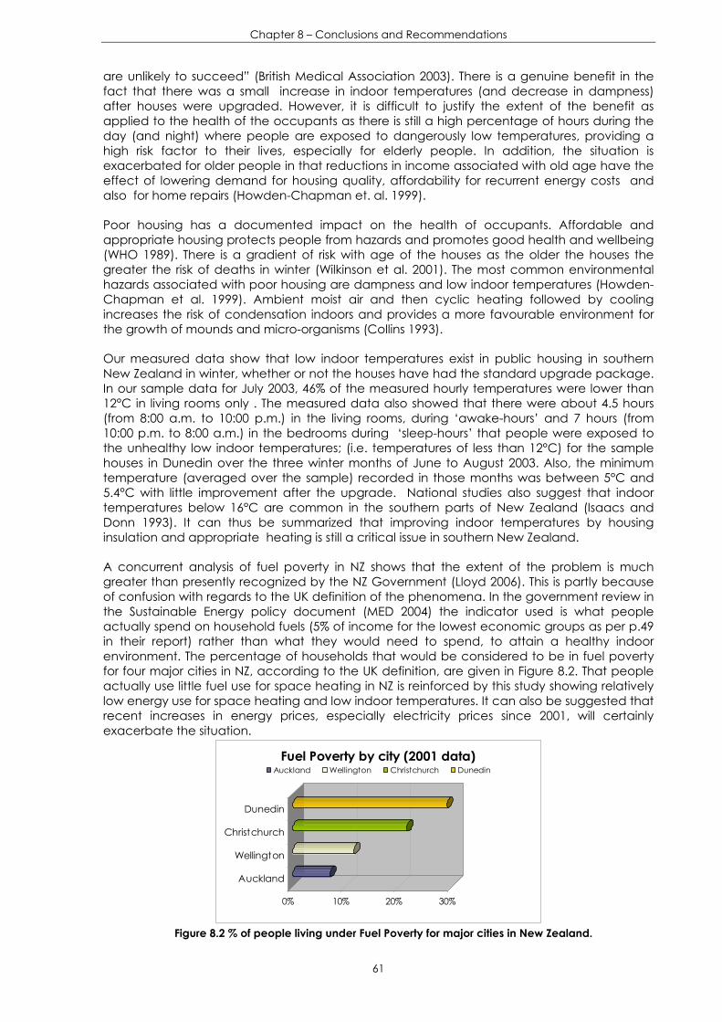
Chapter 8 – Conclusions and Recommendations
61
are unlikely to succeed” (British Medical Association 2003). There is a genuine benefit in the fact that there was a small increase in indoor temperatures (and decrease in dampness) after houses were upgraded. However, it is difficult to justify the extent of the benefit as applied to the health of the occupants as there is still a high percentage of hours during the day (and night) where people are exposed to dangerously low temperatures, providing a high risk factor to their lives, especially for elderly people. In addition, the situation is exacerbated for older people in that reductions in income associated with old age have the effect of lowering demand for housing quality, affordability for recurrent energy costs and also for home repairs (Howden-Chapman et. al. 1999).
Poor housing has a documented impact on the health of occupants. Affordable and appropriate housing protects people from hazards and promotes good health and wellbeing (WHO 1989). There is a gradient of risk with age of the houses as the older the houses the greater the risk of deaths in winter (Wilkinson et al. 2001). The most common environmental hazards associated with poor housing are dampness and low indoor temperatures (Howden-Chapman et al. 1999). Ambient moist air and then cyclic heating followed by cooling increases the risk of condensation indoors and provides a more favourable environment for the growth of mounds and micro-organisms (Collins 1993).
Our measured data show that low indoor temperatures exist in public housing in southern New Zealand in winter, whether or not the houses have had the standard upgrade package. In our sample data for July 2003, 46% of the measured hourly temperatures were lower than 12°C in living rooms only . The measured data also showed that there were about 4.5 hours (from 8:00 a.m. to 10:00 p.m.) in the living rooms, during ‘awake-hours’ and 7 hours (from 10:00 p.m. to 8:00 a.m.) in the bedrooms during ‘sleep-hours’ that people were exposed to the unhealthy low indoor temperatures; (i.e. temperatures of less than 12°C) for the sample houses in Dunedin over the three winter months of June to August 2003. Also, the minimum temperature (averaged over the sample) recorded in those months was between 5°C and 5.4°C with little improvement after the upgrade. National studies also suggest that indoor temperatures below 16°C are common in the southern parts of New Zealand (Isaacs and Donn 1993). It can thus be summarized that improving indoor temperatures by housing insulation and appropriate heating is still a critical issue in southern New Zealand.
A concurrent analysis of fuel poverty in NZ shows that the extent of the problem is much greater than presently recognized by the NZ Government (Lloyd 2006). This is partly because of confusion with regards to the UK definition of the phenomena. In the government review in the Sustainable Energy policy document (MED 2004) the indicator used is what people actually spend on household fuels (5% of income for the lowest economic groups as per p.49 in their report) rather than what they would need to spend, to attain a healthy indoor environment. The percentage of households that would be considered to be in fuel poverty for four major cities in NZ, according to the UK definition, are given in Figure 8.2. That people actually use little fuel use for space heating in NZ is reinforced by this study showing relatively low energy use for space heating and low indoor temperatures. It can also be suggested that recent increases in energy prices, especially electricity prices since 2001, will certainly exacerbate the situation.
0% 10% 20% 30%
Auckland
Wellington
Christchurch
Dunedin
Fuel Poverty by city (2001 data)Auckland Wellington Christchurch Dunedin
Figure 8.2 % of people living under Fuel Poverty for major cities in New Zealand.

Chapter 8 – Conclusions and Recommendations
62
The conclusion must be that deleterious health effects will result from such low temperatures, especially for occupants in the over 65 years age group. In addition, the present low levels of warmth in southern New Zealand homes and the long pay-back periods, of as much as 10 years for the upgrade, may make this energy efficiency measure not so attractive on a purely financial basis.
In terms of energy reduction and the associated CO2 mitigation, again our findings are consistent with the 1976 NZ Statistics report in that the savings in electricity use found at between 6 and 10% may only just be statistically significant.
In terms of water heating, the poor improvement in energy efficiency noticed after the upgrade was due to the low implementation of cylinder wraps. However, according to the HEEP study wrapped cylinders provided a significant reduction of the standing heat losses in their monitored houses, showing evidence that “Cylinder wraps clearly do work” (Isaac, N. et. al 2005).
The reason for the low level of thermal comfort improvement is suggested to be that the simple insulation upgrade, involving only one aspect of the building fabric, for the poorly built and not well heated public HNZC housing was not a complete solution. If improving indoor thermal comfort, and at the same time making energy efficiency at homes was the goal, then more intensive housing insulation measures, or better home energy efficiency technologies would need to be applied. Considerably larger Government subsidies, possibly including complete replacement of the older poorer public housing and subsidized space heating appliances, are likely to be needed to reach satisfactory health goals and promote energy efficiency in the residential area.
8.2 Future Work/Recommendations
Further work will need to be completed in order to firm up on any recommendations that may lead to the solution of some of the questions posed. In particular we intend to progress the computer modelling to look at alternative scenarios for improved upgrades. In addition, we intend to complete further field work looking at installing double glazing and high efficiency light bulbs. We are also planning the complete refurbishment of up to two HNZC houses up to the present (1996) building standards to quantify the improved thermal environment and to detail the costs of completing the upgrade. Further investigations will also take into the account possible mass transfer of water vapour within the wall cavity.
Some recommendations can be made immediately, however, including:
• Unwanted air ingress was a common problem most occupants complained during the survey. Leaky houses with regards to air ingress will result in more heat loss and consume more energy. It is thus recommended that ‘Blower door’ tests be done before and after upgrades in order to estimate the improvement in air leakage rates in the houses. A minimum rate of 0.75 ACH after the upgrade should be adopted.
• Hot water heaters are the biggest single residential home energy consumer (specifically because of very low space heating use) taking about 35% of the household annual electricity consumption. The number of houses that could accept the insulated cylinder wraps in the study homes was extremely small at 2%. A program should be put in place to replace the earlier B, C and D grade cylinders entirely, and relocating the cylinder if necessary so a wrap can be accommodated. In addition, as New Zealand gets reasonably good solar radiation across the country, promoting solar water heating or hot water heat pumps in the residential sector has considerable potential and could significantly reduce energy consumption nationwide. Ways of introducing a subsidized solar heating package (including heat pump hot water systems) into public rental housing should be investigated. Finally, adjusting the

Chapter 8 – Conclusions and Recommendations
63
thermostat for hot water cylinders should be a mandatory component of any upgrade process.
• It was clear that the homes in the study were grossly under-heated. An adequate indoor thermal environment will not be reached using improved insulation unless this situation is changed. It is recommended that ways to encourage efficient space heating in HNZC homes be investigated, including the installation of subsidized equipment such as space heating heat pumps and energy efficient wood burners if necessary. In this regard it is thought essential that all existing open fires be sealed or replaced with energy efficient appliances.
• The use of thermal curtains improved the thermal performance of the one test house by more than the HNZC standard upgrade. Consideration should be given to providing curtains with pelmets instead of applying ceiling insulation to houses for the remainder of the upgrade program. It is also likely that under floor insulation with fibreglass batts will be of greater benefit than the under floor foil insulation but this will be confirmed in the next set of studies to be undertaken.

References
64
References ASHRAE (2001). 2001 ASHRAE Handbook- Fundamentals (SI), American Society of Heating,
Refrigerating, and Air-Conditioning Engineers. 01-Jan-2001. Bassett, M. (1995). A Practical Study of Retrofit Airtightening Old Houses for Energy Efficiency.
Wellington, New Zealand, BRANZ. BRANZ (2000). The 'Annual Loss Factor" Method- A Design Tool for Energy-efficient Houses.
Wellington, Building Research Association of New Zealand. BRANZ (2001). Thermal performance of Buildings with heavy walls. Wellington, Building
Research Association of New Zealand. British Medical Association (2003) Housing and Helath - Building for the future, p30 Close, D. J., H. Suehrcke, A. Masatto. (1995) "The Effect Of Water Vapour Transfer On Natural
Convection Building Cavities". Proceedings of Building Simulation '95: 1-6. Townsville, Australia.
Collins, K. J. (1993). "Cold and Heat-related Illness in the Indoor Environment in Unhealthy Housing: Research Remedies and Reform." E and F.N. Spon, London: 117-140.
DOS (1973). Report on the Survey of Household Electricity Consumption 1971-72. Wellington, Department of Statistics, New Zealand.
DOS (1976). Survey of Household Electricity Consumption 1971-72: Report on the Temperature/ Insulation Study. Wellington, Department of Statistics, New Zealand.
EECA (2000). The Dynamics of Energy Efficiency Trends in New Zealand. Wellington, Energy Efficiency and Conservation Authority, New Zealand.
EECA (2001). National Energy Efficiency and Conservation Strategy. Wellington, Energy Efficiency and Conservation Authority, New Zealand.
HNZC (2001). Energy Efficiency Retro-fit Program, HNZC Housing Spec - Maintenance, Housing New Zealand Corporation, New Zealand.
HNZC (2003). Housing New Zealand Corporation, Wellington, New Zealand. http://www.hnzc.co.nz/.
Hoger W. (2000) Energy Efficient Building Design, Renewable Energy Centre, Brisbane Institute of TAFE. Australia.
Home (2005) Third edition. A joint initiative of the Australian Government and the design and construction industries. Commonwealth of Australia, http://www.greenhouse.gov.au/.
Howden-Chapman, P., Signal, L and Crane, J. (1999). "Housing and Health in Older People: Ageing in Place" Social Policy Journal of New Zealand(13).
Howden-Chapman, P., et. al. (2003). "The Housing, Insulation and Health Study" http://hrc.govt.nz/.
Howden-Chapman, P., Matheson, A., Crane, J., Viggers, H., Cunningham, M., Blakely, T., O'Dea, D., Cunningham, C., Woodward, A., Seville-Smith, K., Baker, M., Waipara, N., Kennedy, M., Davie,. G. (2004). "Retrofitting houses with insulation to reduce health inequalities: A community based randomised trial"
IES (2001). Virtual Environment. Glasgow, Integrated Environmental Solutions Ltd, UK. Isaacs, N.P., Amitrano, L., Camilleri, M., Pollard, A. and Stoecklein, A. (2003). Energy Use in
New Zealand Households: Report on the Year 7 Analysis for the Household Energy End-use Project (HEEP). BRANZ (Study Report SR 122) Wellington, New Zealand.
Isaacs, N.P., Amitrano, L., Camilleri, M., French, L., Pollard, A., Saville-Smith, K., Fraser, R. and Rossouw, P. (2004). Energy Use in New Zealand Households: Report on the Year 8 Analysis for the Household Energy End-use Project (HEEP). BRANZ (Study Report SR 133) Wellington, New Zealand.
Isaacs, N., Camilleri, M., French, L., Pollard A., Saville-Smith, K., Fraser, R., Rossouw, P. and Jowett, J.,(2005). Energy Use in New Zealand Households: Report on the Year 9 Analysis for the Household Energy End-use Project (HEEP). BRANZ (Study Report SR 141) Wellington, New Zealand.
Isaacs, N., Donn, M. (1993). "Health and Housing- Seasonality in New Zealand Mortality" Australian Journal of Public Health 17(1).
Infiltec (1995-2004) DM4 Dual Digital Micro-manometer User's Manual. Version 6. http://www.infiltec.com/.

References
65
Lloyd, C.R. and S. Shannon (2003). Impact of Housing on Health in Dunedin New Zealand. University of Otago, Dunedin, New Zealand.
Lloyd, C.R. (2006) Fuel Poverty in New Zealand: Dunedin, Physics Department, New Zealand. To be published Social Policy Journal of New Zealand.
MED (Jul. 2003). Energy Data File. Wellington, Ministry of Economic Development, New Zealand.
MED (2004). Energy Data File. Wellington, Ministry of Economic Development, New Zealand. NIWA (2004a). Residential Carbon Dioxide Calculator, National Institute of Water &
Atmospheric Research, New Zealand. http://www.niwa.co.nz/. NIWA (2004b). The Climate of New Zealand, National Institute of Water & Atmospheric
Research, New Zealand. http://www.niwa.co.nz/edu/resources/climate/overview/. NZBC H1(1977) New Zealand Building Code. Building Industry Authority. Wellington, New
Zealand. NZS 4214 (1977) New Zealand Standard: Methods of determining the total thermal resistance
of parts of buildings, NZS4218:1977. Wellington, Standards New Zealand. NZS 4218 (1996). New Zealand Standard: Energy Efficiency - Housing and Small Building
Envelope, NZS4218:1996. Wellington, Standards New Zealand. Rankine, J. (2005) "Housing and Health in Auckland", Auckland Regional Public Health Board,
Auckland, New Zealand. Rossouw, P. (2002). New Zealand Building Stock Dynamics and NEECS Initiatives. Dunedin,
New Zealand. Schipper, L., Unander F, Marie-Lilliu, C, Walker I, Urtishaw, S. 2000. Energy Use in New Zealand
in an International Perspective: Comparison of Trends Through the Mid 1990s. Paris: Int. Energy Agency/Wellington, NZ: ECCA .
Schrock, D. W. (1997). Load Shape Development. Tulsa Oklahoma, PennWell Publishing Company, USA.
Shen M. (2004) "Monitoring of the Energy Efficiency of State Houses in Southern New Zealand". University of Otago, Dunedin, New Zealand.
Staley, H. and Howden-Chapman P. (2004) "A healthy return from investing in insulation" Presentation to governments officials, Wellington, New Zealand.
STNZ (2004). Statistics New Zealand Website. Wellington, http://www.stats.govt.nz/. Stoecklein, A., Pollard, A., Camilleri, M., Amitrano, L., Isaacs, N.P., Pool, F. and Clark, S. (ed)
(2001). Energy Use in New Zealand Households: Report on the Year 5 Analysis for the Household Energy End-use Project (HEEP). Wellington, BRANZ, New Zealand.
Szokolay, S.V. (2004) "Introduction to Architectural Science, The basis of Sustainable Design" Architectural Press, UK.
WHO (1985). Health Impact of Low Indoor Temperatures. Copenhagen, World Health Organization.
WHO (1989). Health Principles for Housing. Geneva. Wilkinson, P., Armstrong, B., Landon, M., (2001) The impact of Housing Conditions on Excess
Winter Deaths. London, Environmental Epidemiology Unit, London School of Hygiene & Tropical Medicine, United Kingdom.

APPENDIX A
I
Air Tightness of Surveyed Houses in Dunedin
“Blower Door” Tests In order to measure the amount of heat lost through air leakage, blower door tests were performed on 34 of the survey state houses in Dunedin. The specific device used was an Infiltec Model E-3 Blower Door manufactured in the US. The use of such tests is an approach to identifying and controlling air infiltration, they also provide a way to quantify air flow and the resulting heat loss (see for instance: Building Ventilation, Theory and Measurement, by David Etheridge and Mats Sandberg, Wiley, 1996). A blower door consists in a fan mounted in an adjustable panel that temporarily fits in a doorway. The unit then pressurizes (blows into) or depressurizes (blow out of) the house, typically forcing a 50 Pascals pressure difference. This controlled airflow can be used to identify specific leaks. The test generates an estimate of “air changes per hour” (ACH) of the house under normal winter conditions by multiplying the 50 Pa air flow buy a multiplier which in the present case was 1/14. Doors and windows to the outside were closed while all interior doors were opened. Because open fires were blocked to prevent intrusion of soot from the chimney into the house, the tests did not give accurate results for houses with such openings. Wind is usually the major driving force in infiltration, so it is reasonable to expect higher infiltration rates in windy areas. Location and surrounding of the houses would somehow affect on how they are exposed to wind and the amount of air infiltration that is occurring in the leakage process of each one. Of a total of 34 houses measured in Dunedin using the blower door system, the average infiltration was found to be 0.82 ACH/hour. As it can be seen in the chart there are few houses with less than 0.5 Ach/h and just one was identified to have over 1.5ARCH/h. Most of the houses were between 0.6 and 1.0 ACH/hr. Very air tight houses have average heating season infiltration rates below 0.1 ACH/hr and very leaky houses are above 1.0 ACH/hr. Houses in this case are into the acceptable average but lowering the amount of air leakage would improve the levels of heat lost through this means.
Histogram for the Hourly Air Change Rate
0
1
2
3
4
5
6
7
0.3
0.4
0.5
0.6
0.7
0.8
0.9 1
1.1
1.2
1.3
1.4
1.5
1.6
1.7
1.8
1.9 2
More
Air Change / hr
Freq
uenc
y
AVERAGE

APPENDIX B
II
Energy Efficiency -Household Survey Part A
Location of House ……………………………………………………………………………………………………………………… Occupants Name…………………………………………………………………Phone #……………………………………….. Surveyors …………………………………………………………………………………………………………………………………….
1.0 General
1.1 Number of occupants usually living in the house …………………..in the house 1.2 Number of years living in this house……………….
2.0 Energy Consumption
2.1 Average winter electricity bill………. $/ month: Average summer electricity bill …….$/month
2.2 Average winter wood use……………….cm Average summer wood use ………………………cm
2.3 Gas (LPG) usage Winter ……………………………kg Summer ………………………………kg
2.4 Coal use in Winter ………………………..kg (or $) Summer…………………………kg
3.0 Energy Use 3.1 Main space heating? (1) Type …………… ……Location …………. Winter………………(h) Summer ……………(h) 3.2 Other heaters (2) Type …………… ……Location …………. Winter………………(h) Summer ……………(h) 3.3 Other heaters (3) Type …………… ……Location …………. Winter………………(h) Summer ……………(h) 3.4 Other heaters ( 4) Type …………… ……Location …………. Winter………………(h) Summer ……………(h)
APPENDIX B
III
3.5 Hot water heater type ………………………………… Power rating………………………… Capacity……………………… 3.6 Hot water temperature …………… Cold water temperature………………Shower flow rate @ 40 oC……………………l/m 3.7 Approximate hours of shower use /day…………………………. 3.8 Hours of use/day for TV…………… refrigerator……….clothes washer…………clothes dryer, dishwasher………..micro wave………..cooking stove………….ventilation fan………….lights other……………………..
4.0 Other
4.1 Approximate weekly income for the household ……………………. $/ p.w. 5.0 Health, Temperature, and Comfort 5.1 Is your house at a comfortable temperature in Winter…………… Summer……………….. 5.2 Do you experience mold or damp in your house?………………………….. If so where? ……………………..
5.3Have you experienced any draughts in the house?……………………… Where? 5.4 Have any family members been sick during the last winter?………………………… Type of illness…………………………………………………………………………………. 6.0 Other
6.1 Approximate weekly income for the household ……………………. $/ p.w. 6.2What do you think will be the benefits of upgrading your house for better energy efficiency : ……………………………………………………………………………………………………………………………………………………………………………………………………………………………………………………………………………………………………………………………………………………………………………………………………………………………………………………………………………………………….
Thank you very much for your cooperation!

APPENDIX C
IV
Energy Efficiency -Household Survey Part B
Location of House ……………………………………………………………………………………………………………………… Occupants Name…………………………………………………………………Phone #……………………………………….. Surveyor …………………………………………………Date surveyed………………………………………………………
Loggers ibutton (1) Ser#………………………………………………… Location……………………………………………… (2) Ser #………………………………………………. Location……………………………………………… Energy pulse counter (3)………………………………………………………….. Location……………………………………………… Hot water hour meter (4)………………………………………………………… Location……………………………………………… Hobo temperature humidity(5)………………………………………………. Location ……………………………………………..
1. The Building and its Structure 1.1 Age of house……………… Number of stories………….. Ceiling height…………………………… 1.2 Heater (1) type …………………..Heater (2) type ………………………… Heater (3) type…………………
1.3 Heating cycle hours in Morning …………………. Evening………………………… Day………………… Night………………
1.4 Total floor area is …………………m2. Type of floor construction …………………Insulated………………….
1.5 Floor covering type (1) ………………….area …………. Floor covering type (2) ………………………area………………….
2.0 The outside wall material (1) ................................. thickness…………………………Insulation............................… 2.1 The outside wall material (2) ................................. thickness…………………………Insulation............................…
3.0 Wall area ………………………….N……………………….NW…………………………W………………………..SW
…………………………….S………………………...SE…………………………E………………………..NE

APPENDIX C
V
4.0 Window area ……………………...N……………………….NW…………………………W………………………..SW …………………………….S………………………...SE…………………………E………………………..NE Shading of windows ……………………………………………………………………………………………………………. 5.0 Window construction……………………………………………………….. 6.0 Roof Construction……………………………………… Roof area……………………………………….. .
5.0 Roof Insulation ………………………………………… Skylight area…………………………………….
6.0 Air Leakage ……………………………………… Open fires…………………………Flues……………………