chapter v - middle east technical...
TRANSCRIPT
Ugur HALICI - METU EEE - ANKARA 11/18/2004
EE543 - ANN - CHAPTER 5 1
Annealing by Stochastic Annealing by Stochastic Neural Networks for Optimization Neural Networks for Optimization
CHAPTER CHAPTER VV
CHAPTER CHAPTER V :V : Annealing by Stochastic Annealing by Stochastic NNsNNs for Optimizationfor Optimization
Introduction
Two major classes of optimization techniques are the deterministic gradient methods and stochastic annealing methods.
Gradient descent algorithms are greedy algorithms, which are subject to a fundamental limitation of being easily trapped in local minima of the cost function.
Hopfield networks usually converge to a local minimum of energy function. This problem is overcome by the use of stochastic annealing algorithms since they provide opportunity to escape from local minima.
Boltzmann machine has capability of escaping local minima through a relaxation technique based on simulated annealing

Ugur HALICI - METU EEE - ANKARA 11/18/2004
EE543 - ANN - CHAPTER 5 2
CHAPTER CHAPTER V :V : Annealing by Stochastic Annealing by Stochastic NNsNNs for Optimizationfor Optimization
IntroductionHowever, the use of simulated annealing is also responsible for an excessive computation time requirement that has hindered experimentation with the Boltzmannmachine [Hinton et al 83].
In order to overcome this major limitation of the Boltzmann machine mean field approximation may be used, according to which the binary state stochastic neurons of the Boltzmann machine are replaced by deterministic mean values [Amit et al 85].
The Gaussian machine [Aiker et al 91], is another stochastic neural network developed over the continuous Hopfield model allowing escape from local minima.
CHAPTER CHAPTER V :V : Annealing by Stochastic Annealing by Stochastic NNsNNs for Optimizationfor Optimization
5.1. Statistical Mechanics and the Simulated Annealing
Consider a physical system with a set of states χ={x}, each of which has energy E(χ).
For a system at a temperature T>0, its state χ varies with time, and quantities such as E(χ) that depend on the state fluctuates.
After a change of parameters, the fluctuations has, on the average a definite direction such that the energy E(χ) decreases.
However, some times later, any such trend ceases and the system just fluctuates around a constant average value. Then we say that the system is in thermal equilibrium.
Ugur HALICI - METU EEE - ANKARA 11/18/2004
EE543 - ANN - CHAPTER 5 3
CHAPTER CHAPTER V :V : Annealing by Stochastic Annealing by Stochastic NNsNNs for Optimizationfor Optimization
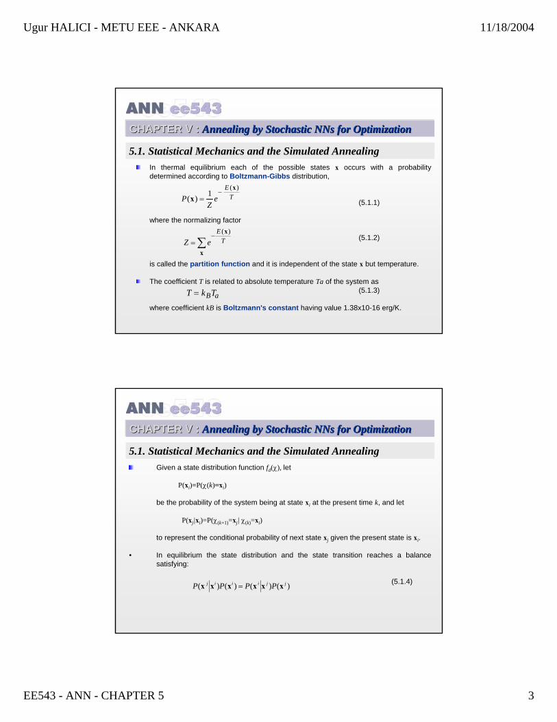
5.1. Statistical Mechanics and the Simulated AnnealingIn thermal equilibrium each of the possible states x occurs with a probability determined according to Boltzmann-Gibbs distribution,
(5.1.1)
where the normalizing factor
(5.1.2)
is called the partition function and it is independent of the state x but temperature.
The coefficient T is related to absolute temperature Ta of the system as(5.1.3)
where coefficient kB is Boltzmann's constant having value 1.38x10⁻¹⁶ erg/K.
PZ
eE
T( )( )
xx
=−1
Z eE
T=−
∑( )x
x
T k TB a=
CHAPTER CHAPTER V :V : Annealing by Stochastic Annealing by Stochastic NNsNNs for Optimizationfor Optimization
5.1. Statistical Mechanics and the Simulated AnnealingGiven a state distribution function fd(χ), let
P(xi)=P(χ(k)=xi)
be the probability of the system being at state xi at the present time k, and let
P(xj|xi)=P(χ(k+1)=xj| χ(k)=xi)
to represent the conditional probability of next state xj given the present state is xi.
• In equilibrium the state distribution and the state transition reaches a balance satisfying:
(5.1.4))()()()( jjiiij PPPP xxxxxx =

Ugur HALICI - METU EEE - ANKARA 11/18/2004
EE543 - ANN - CHAPTER 5 4
CHAPTER CHAPTER V :V : Annealing by Stochastic Annealing by Stochastic NNsNNs for Optimizationfor Optimization
5.1. Statistical Mechanics and the Simulated AnnealingRemember:
(5.1.1)
• Therefore, in equilibrium the Boltzmann Gibbs distribution given by equation (5.1.1) results in:
(5.1.6)
where
∆E=E(x j)-E(x i).
TEij
eP /1
1)( ∆+=xx
PZ
eE
T( )( )
xx
=−1
CHAPTER CHAPTER V :V : Annealing by Stochastic Annealing by Stochastic NNsNNs for Optimizationfor Optimization
5.1. SM & SA: Metropolis Algorithm
The Metropolis algorithm provides a simple method for simulating the evolution of physical system in a heat bath to thermal equilibrium [Metropolis et al].
It is based on Monte Carlo Simulation technique, which aims to approximate the expected value <g(.)> of some function g(χ) of a random vector with a given density function fd(.).

Ugur HALICI - METU EEE - ANKARA 11/18/2004
EE543 - ANN - CHAPTER 5 5
CHAPTER CHAPTER V :V : Annealing by Stochastic Annealing by Stochastic NNsNNs for Optimizationfor Optimization
5.1. SM & SA: Metropolis Algorithm
For this purpose several χ vectors, say χ=Xk, k=1..K, are randomly generated according to the density function fd(χ) and then Yk is found as Yk=g(Xk).
By using the strong law of large numbers:
(5.1.7)
the average of generated Y vectors can be used as an estimate of <g(.)> [Sheldon 1989].
>>=<=<∑∞→)(lim 1 χYY gkk
kKK
CHAPTER CHAPTER V :V : Annealing by Stochastic Annealing by Stochastic NNsNNs for Optimizationfor Optimization
5.1. SM & SA: Metropolis AlgorithmIn each step of the Metropolis algorithm, an atom (unit) of the system is subjected to a small random displacement, and the resulting change E in the energy of the system is observed.
If E ≤ 0, then the displacement is accepted,
If E >0, the configuration with the displaced atom is accepted with a probability given by:
(5.1.8)
Provided enough number of transitions in the Metropolis algorithm, the system reaches thermal equilibrium.
It effectively simulates the motions of the atoms of a physical system at temperature T obeying Boltzmann-Gibbs distribution provided previously.
P E e E T( ) /∆ ∆= −

Ugur HALICI - METU EEE - ANKARA 11/18/2004
EE543 - ANN - CHAPTER 5 6
CHAPTER CHAPTER V :V : Annealing by Stochastic Annealing by Stochastic NNsNNs for Optimizationfor Optimization
5.1. SM & SA: Effects of T on distributionNotice that In Boltzmann-Gibbs distribution
P(xi) > P(xj) ⇔ E(xi) < E(xj)
This property is independent of the temperature, although the discrimination becomes more apparent as the temperature decrease. (Figure 5.1)
Energy
Prob
abili
ty
High Temprature
Low Temprature
Figure 5.1 Relation Between temperature and probability of the State
CHAPTER CHAPTER V :V : Annealing by Stochastic Annealing by Stochastic NNsNNs for Optimizationfor Optimization
5.1. SM & SA: Effects of T on distribution
However, if the temperature is too high, all the states will have a similar level of probability.
On the other hand, as T→ 0, the average state gets closer to the global minimum.
In fact, with a low temperature, it will take a very long time to reach equilibrium and, more seriously, the state is more easily trapped by local minima.

Ugur HALICI - METU EEE - ANKARA 11/18/2004
EE543 - ANN - CHAPTER 5 7
CHAPTER CHAPTER V :V : Annealing by Stochastic Annealing by Stochastic NNsNNs for Optimizationfor Optimization
5.1. SM & SA: Effects of T on distribution
Therefore, it is necessary to start at a high temperature and then decrease it gradually. Correspondingly, the probable state then gradually concentrate around the globally minimum (Figure 5.2).
Figure 5.2 The energy levels adjusted for high and low temperature
High Temprature
Low Temprature
CHAPTER CHAPTER V :V : Annealing by Stochastic Annealing by Stochastic NNsNNs for Optimizationfor Optimization
5.1. SM & SA: Metallurgical Annealing
This has an analogy with metallurgical annealing, in which a body of metal is heated near to its melting point and is then slowly cooled back down to room temperature.
This process eliminates dislocations and other crystal lattice disruptions by thermal agitation at high temperature.
Furthermore, it prevents the formation of new dislocations by cooling the metal very slowly. This provides necessary time to repair any dislocations that occur as the temperature drops.
The essence of this process is that global energy function of the metal will eventually reach a global minimum value.
If the material is cooled rapidly, its atoms are often captured in unfavorable locations in the lattice

Ugur HALICI - METU EEE - ANKARA 11/18/2004
EE543 - ANN - CHAPTER 5 8
CHAPTER CHAPTER V :V : Annealing by Stochastic Annealing by Stochastic NNsNNs for Optimizationfor Optimization
5.1. SM & SA: Metallurgical Annealing
In order to escape from local minima and to have the lattice in the global energy minimum, the thermal fluctuations can be enhanced by reheating the material until energy-consuming local rearrangements occur at a reasonable rate.
A great deal of experience is required to perform the annealing in an optimal way. If the temperature is decreased quickly, some thermal fluctuations are frozen in. On the other hand, if one proceeds too slowly, the process never ends.
The amazing thing about annealing is that the statistical process of thermal agitation leads to approximately the same final energy state.
This result is independent of the initial condition of the metal and any of the details of the statistical annealing process.
The mathematical concept of simulated annealing derives from an analogy with this physical behavior.
CHAPTER CHAPTER V :V : Annealing by Stochastic Annealing by Stochastic NNsNNs for Optimizationfor Optimization
5.1. SM & SA: Simulated AnnealingThe simulated annealing algorithm, is a variant of the Metropolis algorithm in which the temperature is time dependent.
The annealing schedule developed by [Kirkpatrick et al 1983] is as follows.
SIMULATED ANNEALING
Step 1. Set Initial values: assign a high value to temperature as T(0)= T0, decide on constants κT, A and S, Typical values for which are 0.8< κT<0.99, A=10, and S=3.
Step 2. Decrement the temperature: , where κT is a constant smaller but close to unity.
Step 3. Attempt enough number of transitions at each temperature, so that there are A accepted transitions per experiment on the average.
Step 4. Stop if the desired number of acceptances is not achieved at S successive temperatures else repeat steps 2 and 3.
)1()( −= kTkT Tκ

Ugur HALICI - METU EEE - ANKARA 11/18/2004
EE543 - ANN - CHAPTER 5 9
CHAPTER CHAPTER V :V : Annealing by Stochastic Annealing by Stochastic NNsNNs for Optimizationfor Optimization
5.1. SM & SA: Simulated Annealing
Provided the initial temperature T0 is high enough, if T(k) at iteration k is chosen such that it satisfies
(5.1.9)
then the system will converge to the minimum energy configuration [Geman and Geman 84].
A very important property of simulated annealing is its asymptotic convergence.
The main drawback of simulated annealing is the large amount of computational time necessary for stochastic relaxation.
T k Tk
( )log( )
≥+
01
CHAPTER CHAPTER V :V : Annealing by Stochastic Annealing by Stochastic NNsNNs for Optimizationfor Optimization
5.2. Boltzmann Machine
Boltzmann machine [Hinton et al 83] is a connectionist model having stochastic nature.
The structure of the Boltzmann machine is similar to Hopfield network, but it adds some probabilistic component to the output function.
It uses simulated annealing concepts, in spite of the deterministic nature in state transition of the Hopfield network [Hinton et al 83, Aarts et al 1986, Allwright and Carpenter 1989, Laarhoven and Aarts 1987].
A Boltzmann machine can be viewed as a recurrent neural network consisting of Ntwo-state units.
Depending on the purpose, the states can be chosen from binary space, that is x{0,1}N or from bipolar space x{-1,1}N .

Ugur HALICI - METU EEE - ANKARA 11/18/2004
EE543 - ANN - CHAPTER 5 10
CHAPTER CHAPTER V :V : Annealing by Stochastic Annealing by Stochastic NNsNNs for Optimizationfor Optimization
5.2. Boltzmann Machine
The objective of a Boltzmann machine is to reach the global minimum of its energy function, which is the state having minimum energy.
Similar to simulated annealing algorithm, the state transition mechanism of Boltzmann Machine uses a stochastic acceptance criterion, thus allowing it to escape from its local minima.
In a sequential Boltzmann machine, units change their states one by one, while they change state all together in a parallel Boltzmann machine
CHAPTER CHAPTER V :V : Annealing by Stochastic Annealing by Stochastic NNsNNs for Optimizationfor Optimization
5.2. Boltzmann Machine
The energy function of the Boltzmann machine is:
(5.2.1)
The connections are symmetrical by definition, that is wij=wji. Furthermore in the bipolar case, the convergence of the machine requires wii=0.
However in the binary case self-loops are allowed.
E w x x xij ij
N
i
Nj i
i
Ni( )x = − −∑∑ ∑1
2θ

Ugur HALICI - METU EEE - ANKARA 11/18/2004
EE543 - ANN - CHAPTER 5 11
CHAPTER CHAPTER V :V : Annealing by Stochastic Annealing by Stochastic NNsNNs for Optimizationfor Optimization
5.2. Boltzmann Machine
Let X denote the state space of the machine, that is the set of all possible states.
Among these, the state vectors differing only one bit are called neighboring states.
The neighborhood Nx⊂X is defined as the set of all neighboring states of x.
CHAPTER CHAPTER V :V : Annealing by Stochastic Annealing by Stochastic NNsNNs for Optimizationfor Optimization
5.2. Boltzmann Machine
Let to denote the neighboring state that is obtained from x by changing the state of neuron j.
Hence, in binary case we have
(5.2.2)
In bipolar case, this becomes:
(5.2.3)
x xx Ni
ji i j
i i j n j= − ∈ ∈=≠
1 0 1ifif ( , ) ,x x x
x xx Ni
ji i j
i i j n j= − ∈ − ∈=≠
ifif ( , ) ,x x x1 1
x j

Ugur HALICI - METU EEE - ANKARA 11/18/2004
EE543 - ANN - CHAPTER 5 12
CHAPTER CHAPTER V :V : Annealing by Stochastic Annealing by Stochastic NNsNNs for Optimizationfor Optimization
5.2. Boltzmann MachineRemember:
• The difference in energy when the global state of the machine is changed from x to is:
(5.2.4)
• Note that the contribution of the connections wkm, for k≠j, m≠j, to E(x) and areidentical, furthermore wij=wij. For the binary case, by using energy equation we obtain
(5.2.5)
x j
∆E E Ej j( ) ( ) ( )x x x x= −
E j( )x
N
ijiijj
j xwxE }1,0{))(12()( ∈+−=∆ ∑ xxx θ
E j( )x
E w x x xij ij
N
i
Nj i
i
Ni( )x = − −∑∑ ∑1
2θ
CHAPTER CHAPTER V :V : Annealing by Stochastic Annealing by Stochastic NNsNNs for Optimizationfor Optimization
5.2. Boltzmann Machine
For the bipolar case it is
(5.2.6)
Therefore, for both of the cases, the change in the energy can be computed by considering only local information.
0,}1,1{))(2()( =−∈+=∆ ∑ iiN
ijiijj
j wxwxE xxx θ
Ugur HALICI - METU EEE - ANKARA 11/18/2004
EE543 - ANN - CHAPTER 5 13
CHAPTER CHAPTER V :V : Annealing by Stochastic Annealing by Stochastic NNsNNs for Optimizationfor Optimization
5.2. Boltzmann Machine
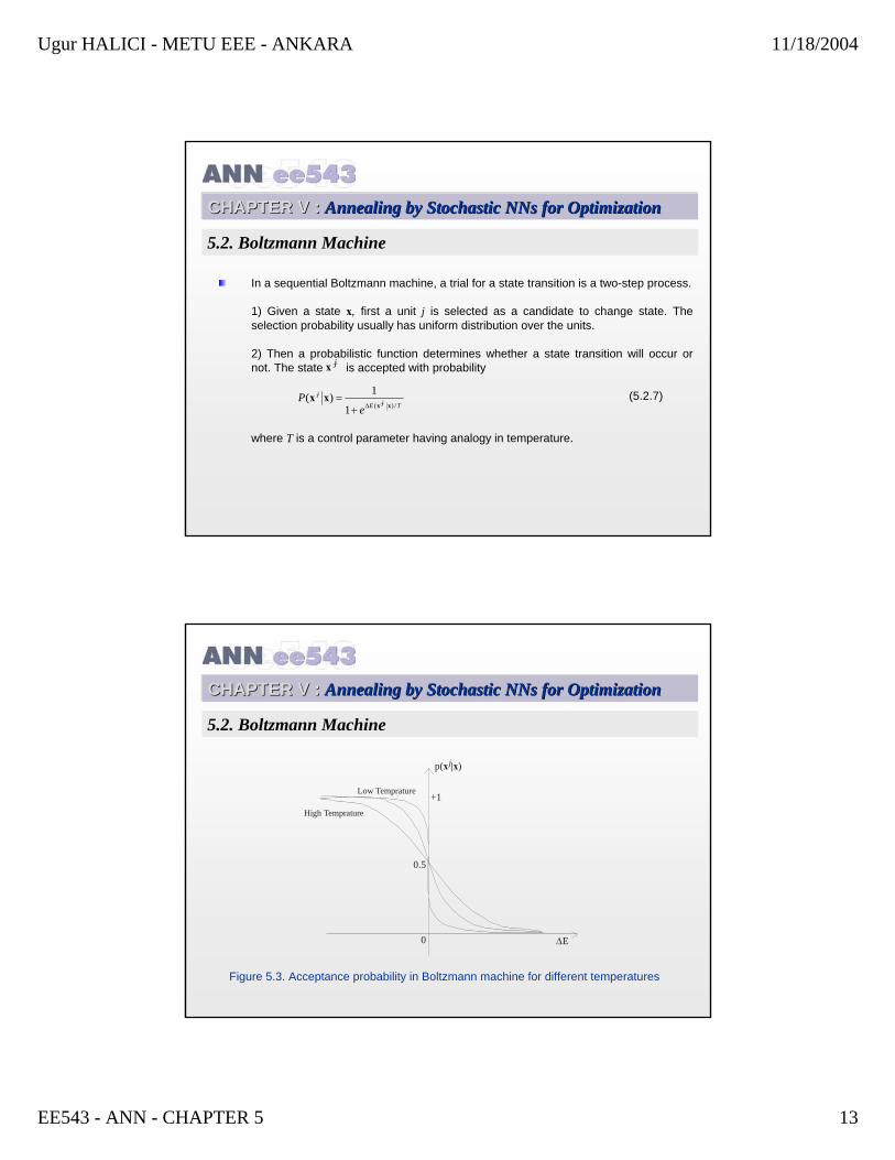
In a sequential Boltzmann machine, a trial for a state transition is a two-step process.
1) Given a state x, first a unit j is selected as a candidate to change state. The selection probability usually has uniform distribution over the units.
2) Then a probabilistic function determines whether a state transition will occur or not. The state is accepted with probability
(5.2.7)
where T is a control parameter having analogy in temperature.
x j
TjE
j
eP
/)(1
1)(xx
xx∆+
=
CHAPTER CHAPTER V :V : Annealing by Stochastic Annealing by Stochastic NNsNNs for Optimizationfor Optimization
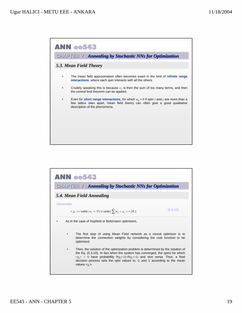
5.2. Boltzmann Machine
Figure 5.3. Acceptance probability in Boltzmann machine for different temperatures
p( )x |x
0.5
+1
0 ∆E
Low Temprature
High Temprature
j

Ugur HALICI - METU EEE - ANKARA 11/18/2004
EE543 - ANN - CHAPTER 5 14
CHAPTER CHAPTER V :V : Annealing by Stochastic Annealing by Stochastic NNsNNs for Optimizationfor Optimization
5.2. Boltzmann Machine
A Boltzmann machine starts execution with a random initial configuration. Initially, the value of T is very large.
A cooling schedule determines how and when to decrement the control parameter T.
As T→ 0, less and less state transitions occur.
If no state transitions occur for a specified number of trials, it is decided that the Boltzmann machine has reached the final state.
CHAPTER CHAPTER V :V : Annealing by Stochastic Annealing by Stochastic NNsNNs for Optimizationfor Optimization
5.2. Boltzmann MachineA state x*∈X is called a locally minimal state, if
(5.2.8)
Let the set of all local minima be denoted by X*.
Note that, a local minimum is a state whose energy can not be increased by a single state transition.
While the Hopfield network is trapped mostly in one of these local minima, the Boltzmann machine can escape from the local minima because of its probabilistic nature.
NjE j ..10*)*( =≥∆ xx

Ugur HALICI - METU EEE - ANKARA 11/18/2004
EE543 - ANN - CHAPTER 5 15
CHAPTER CHAPTER V :V : Annealing by Stochastic Annealing by Stochastic NNsNNs for Optimizationfor Optimization
5.2. Boltzmann Machine
Although the machine asymptotically converges to a global minimum, the finite-time approximation of the Boltzmann Machine does not guarantee convergence to a state with minimum energy.
However, still the final state of the machine will be a nearly minimum one among X*.
Use of Boltzmann machine as a neural optimizer involves two phases as it is explained for the Hopfield network in Chapter 4.
In the first phase, the connection weights are determined. For this purpose, a cost function for the given application is decided. The next step is to determine the connection weights {wij} by comparing the energy function with this cost function.
Then in the second phase, the machine searches the global minimum through the annealing procedure.
CHAPTER CHAPTER V :V : Annealing by Stochastic Annealing by Stochastic NNsNNs for Optimizationfor Optimization
5.3. Mean Field Theory
Although the use of simulated annealing provides for escaping from the local minima, it results in an excessive computation time requirement that has hindered experimentation with the Boltzmann machine.
Not only does simulated annealing require iterations at a sequence of temperatures that defines the annealing cycle but also each iteration requires many sweeps of its own.
In order to overcome this major limitation of the Boltzmann machine, mean field approximation may be used.
In mean field network, the binary state stochastic neurons of the Boltzmannmachine are replaced by deterministic analogue neurons [Amit et al 87].

Ugur HALICI - METU EEE - ANKARA 11/18/2004
EE543 - ANN - CHAPTER 5 16
CHAPTER CHAPTER V :V : Annealing by Stochastic Annealing by Stochastic NNsNNs for Optimizationfor Optimization
5.3. Mean Field Theory
Mean-field approximation is a well-known concept in statistical physics [Glauber63].
In the context of a stochastic machine it would be desirable to know the states of the neurons at all time.
However, in the case of a network with a large number of neurons, the neural states contain vastly more information than what is required in practice.
In fact, to answer the most of the physical questions about the stochastic behavior of the network, we need only to know the average values of neural states or the average products of pairs of neural states.
CHAPTER CHAPTER V :V : Annealing by Stochastic Annealing by Stochastic NNsNNs for Optimizationfor Optimization
5.3. Mean Field TheoryConsider the discrete Hopfield network that we considered previously, where states were restricted to be x{-1,1}N.
Now lets replace the deterministic units in this network by stochastic units [Hinton and Sejnowski 83, Peretto 84] that behave in the following manner:
(5.3.1)
where fT(.) is the sigmoid function:
(5.3.2)
Moreover, T is the pseudo temperature. Such a stochastic unit may be interpreted as ordinary deterministic threshold unit with a random threshold θ drawn from a probability density .
χ iT i
T i
Nwith probability f awithprobability f a
=+− −
∈ −11 1
1 1( )
( )( , )x
f ae
T a T( ) /=+ −
11 2
′fT ( )θ

Ugur HALICI - METU EEE - ANKARA 11/18/2004
EE543 - ANN - CHAPTER 5 17
CHAPTER CHAPTER V :V : Annealing by Stochastic Annealing by Stochastic NNsNNs for Optimizationfor Optimization
5.3. Mean Field TheoryRemember
(5.3.2)
• Notice that the sigmoid function defined by equation (5.3.2) has the property
(5.3.5)
• In the case of the network having a single element, the average value for χ=x1 can be calculated as:
(5.3.6)
1− = −f a f aT T( ) ( )
< >= = + + + = − −
=+
−+
=−
+=
− +
−
−
χ χ χP P
e ee ee e
a T
a T a T
a T a T
a T a T
( ).( ) ( ).( )
tanh( / )
/ /
/ /
/ /
1 1 1 1
11
112 2
f ae
T a T( ) /=+ −
11 2
CHAPTER CHAPTER V :V : Annealing by Stochastic Annealing by Stochastic NNsNNs for Optimizationfor Optimization
5.3. Mean Field Theory
fh(a/T)=tanh(a/T) function has the same kind of shape as fT(.) except that it goes from -1 to 1 instead of 0 to 1. In fact
(5.3.7)
It should be not forgotten that, at a given time, χ itself is still either +1 or -1. It flips back and forth randomly between these two values, taking on one of them more frequently according to fT(a).
f a T a T f ah T( / ) tanh( / ) ( )= = −2 1

Ugur HALICI - METU EEE - ANKARA 11/18/2004
EE543 - ANN - CHAPTER 5 18
CHAPTER CHAPTER V :V : Annealing by Stochastic Annealing by Stochastic NNsNNs for Optimizationfor Optimization
5.3. Mean Field Theory
In the case of many interacting neurons, the problem is not easily solved.
The evolution of a spin, represented by i depends on the activation
(5.3.8)
which involves random variables χj that themselves fluctuate back and forth.
ij
n
jjii w θχα +=∑
=1
CHAPTER CHAPTER V :V : Annealing by Stochastic Annealing by Stochastic NNsNNs for Optimizationfor Optimization
5.3. Mean Field Theory
The basic idea of mean-field approximation is to replace the actual fluctuating activation ∝j for each neuron j in the network by its average <∝j> as:
(5.3.9)
Then, we can compute the average < ∝j > as in the case of single-unit problem:
(5.3.10)
These are still N non-linear equations in N unknowns, but at least they no longer involve stochastic variables
ij
n
jijij
n
jiji ww θχθχα +><≅>+>=<< ∑∑
∑ +><≅><>=<n
jiTjijTii wT )tanh()/tanh( 11 θχαχ
Ugur HALICI - METU EEE - ANKARA 11/18/2004
EE543 - ANN - CHAPTER 5 19
CHAPTER CHAPTER V :V : Annealing by Stochastic Annealing by Stochastic NNsNNs for Optimizationfor Optimization
5.3. Mean Field Theory
• The mean field approximation often becomes exact in the limit of infinite range interactions, where each spin interacts with all the others.
• Crudely speaking this is because ∝i is then the sum of too many terms, and then the central limit theorem can be applied.
• Even for short range interactions, for which wij ≈ 0 if spin i and j are more than a few lattice sites apart, mean field theory can often give a good qualitative description of the phenomena.
CHAPTER CHAPTER V :V : Annealing by Stochastic Annealing by Stochastic NNsNNs for Optimizationfor Optimization
5.4. Mean Field Annealing
• The first step of using Mean Field network as a neural optimizer is to determine the connection weights by considering the cost function to be optimized.
• Then, the solution of the optimization problem is determined by the solution of the Eq. (5.3.10). In fact when the system has converged, the spins for which <χi> > 0 have probability P(χi=1)>P(χi=-1) and vice versa. Thus, a final decision process sets the spin values to -1 and 1 according to the mean values <χi>.
Remember
(5.3.10)
• As in the case of Hopfield or Boltzmann optimizers,
∑ +><≅><>=<n
jiTiijTii wT )tanh()/tanh( 11 θχαχ

Ugur HALICI - METU EEE - ANKARA 11/18/2004
EE543 - ANN - CHAPTER 5 20
CHAPTER CHAPTER V :V : Annealing by Stochastic Annealing by Stochastic NNsNNs for Optimizationfor Optimization
5.4. Mean Field Annealing
• Contrary to simulated annealing, this method is intrinsically parallel by nature.
• The convergence process of the mean field algorithm is purely deterministic and is controlled by a dynamical system. This reduces the computational effort considerably.
• The main drawback of this method is the difficulty in the choice of the parameter T.
• It has no major influence on the quality of the results when it is chosen in a certain range.
• In order to overcome the difficulty in choice of the ambient temperature, mean field annealing is proposed.
CHAPTER CHAPTER V :V : Annealing by Stochastic Annealing by Stochastic NNsNNs for Optimizationfor Optimization
5.4. Mean Field Annnealing
• An approach in mean field annealing consists of annealing during the convergence of the mean field approximation.
• That is, the temperature is decreased slowly, while the coupled mean field equations for the averages <χj > are solved iteratively.
• This can be done simply by using a continuous valued Hopfield network, in which the shape of the sigmoid output function changes as a function of temperature.
• The temperature can be slightly decreased from a high value to a smaller one as soon as each neuron has been updated once.
• The system does not reach a near equilibrium state at any temperature during the convergence process but when the temperature is small enough, the system is frozen in a good stable state.
Ugur HALICI - METU EEE - ANKARA 11/18/2004
EE543 - ANN - CHAPTER 5 21
CHAPTER CHAPTER V :V : Annealing by Stochastic Annealing by Stochastic NNsNNs for Optimizationfor Optimization
5.3. Mean Field Annealing
Another approach [Van den Bout and Miller 88] uses the critical temperature. During cooling process, there is a critical temperature Tc at which the mean field variables <χi> begin to move significantly towards +1 and -1.
The principle is then to estimate theoretically this critical temperature and to let the system evolve at this temperature until equilibrium is reached.
Then one decreases the temperature to near zero and iterates until the system has reached a near equilibrium state.
CHAPTER CHAPTER V :V : Annealing by Stochastic Annealing by Stochastic NNsNNs for Optimizationfor Optimization
5.5. Gaussian Machine
An extension of the mean field annealing is the Gaussian machine, whose structure is the same as continuous the state asynchronous Hopfield network except the following properties:
A Gaussian distributed random noise is added to each input.
The gain of the amplifiers is time- variant.
The total input si to neuron i is given by formula
(5.5.1)
where wji is the synaptic weight between neurons j and i, xj is the output of neuron i, θi is the input bias and ε is a Gaussian distributed random noise having zero mean and σ2 variance.
εθ ++=∑ ij
jii jxws

Ugur HALICI - METU EEE - ANKARA 11/18/2004
EE543 - ANN - CHAPTER 5 22
CHAPTER CHAPTER V :V : Annealing by Stochastic Annealing by Stochastic NNsNNs for Optimizationfor Optimization
5.5. Gaussian Machine
This noise term breaks the determinism of each neuron in the Hopfield network and allows escaping from local minima.
The deviation σ is defined as
(5.5.2)
where k is a constant equal to and T is the pseudo-temperature whose value decreases in time to zero.
kT=σ
π8
CHAPTER CHAPTER V :V : Annealing by Stochastic Annealing by Stochastic NNsNNs for Optimizationfor Optimization
5.5. Gaussian MachineGaussian distribution, which is known also as normal distribution, has the following formula:
(5.5.3)
where µ is the mean and has value 0 in our case.
• The activation value ai of neuron i is changed according to the difference equation
(5.5.4)
where is the time constant that can be set to 1 with no loss of generality.
∆t has the range 0 < ∆t ≤ 1.
f u e u( ) ( ) /= − −12
2 22πσ
µ σ
iii s
at
a+
−=
∆∆
τ

Ugur HALICI - METU EEE - ANKARA 11/18/2004
EE543 - ANN - CHAPTER 5 23
CHAPTER CHAPTER V :V : Annealing by Stochastic Annealing by Stochastic NNsNNs for Optimizationfor Optimization
5.5. Gaussian Machine
For the simulation of the Gaussian machine, [Akiyama et al 91] uses asynchronous neuron updates.
The output value xi is determined by the sigmoid function
(5.5.5)
as defined previously, where 1/A is the gain of the curve and the value of A is decreased in time so that the sigmoid function becomes unit step function.
x
e
i ai=
+−
1
1 Α
CHAPTER CHAPTER V :V : Annealing by Stochastic Annealing by Stochastic NNsNNs for Optimizationfor Optimization
5.5. Gaussian MachineThe activation level A is started from some large value and decreased in time towards zero. A is controlled by the following hyperbolic scheduling:
(5.5.6)
where A0 is the initial value of A and τA is the time constant of the sharpening schedule.
A At A
=+
01 / τ

Ugur HALICI - METU EEE - ANKARA 11/18/2004
EE543 - ANN - CHAPTER 5 24
CHAPTER CHAPTER V :V : Annealing by Stochastic Annealing by Stochastic NNsNNs for Optimizationfor Optimization
5.5. Gaussian Machine
The temperature T is also decreased in time, in turn it decreases the deviation ofthe noise . T is controlled by the following hyperbolic annealing schedule:
(5.5.7)
where T0 is the initial temperature and τT is the time constant of the annealing schedule, which may differ from τA.
The choice of A0, T0, τA and τT for the Gaussian machine for a good performance (in terms of convergence in a shorter time and convergence to a better minimum)is not a trivial task.
T Tt T
=+
01 / τ