chapter 9: fm receivers - n0gsgn0gsg.com/ecfp/ch9_sample.pdfat the conclusion of this chapter, ......
TRANSCRIPT
© 2017 Tom A. Wheeler. Sample for Evaluation. WWW.N0GSG.COM/ECFP 306
Chapter 9: FM Receivers
Chapter 9 Objectives At the conclusion of this Chapter, the reader will be able to: FM is popular as a communications mode because of its superior noise performance
and fidelity, when compared to AM. The operation of AM and FM receivers is very similar; the same familiar circuit techniques are used in both. The primary differences in an FM receiver stem from the relatively high frequencies used for FM transmission (the VHF and UHF bands), and the differences in detector circuitry. FM receivers tend to be more "feature-laden." The addition of circuitry to support FM stereo, SCA, automatic (microcomputer-driven) tuning, and other features adds complexity to the set.
FM is a fundamental technology, like AM. Its techniques are used in satellite and data communications, telemetry (remote measurement), and a score of other non-broadcast applications. A professional with a strong knowledge of FM can go far in communications!
9-1 FM Superheterodyne Receivers
FM receivers use the superheterodyne principle, as shown in Figure 9-1. Recall that a superhet receiver operates by converting the desired incoming RF carrier frequency down to the IF or intermediate frequency, where most of the amplification is provided and receiver bandwidth is defined. The sections of the receiver that are new or different compared to an AM receiver are in blue.
• Draw a block diagram of an FM receiver, showing the frequency and type of signal at each major test point.
• Explain the operation and alignment of Foster-Seeley/Ratio, PLL, and quadrature FM detector circuits.
• Describe the features of noise-suppressing circuits in an FM receiver. • Draw a block diagram of a frequency-synthesized FM receiver. • Trace the signal flow through FM stereo and SCA decoder circuits. • Describe the alignment procedures unique to FM receivers. • Apply basic troubleshooting methods to FM receivers.

© 2017 Tom A. Wheeler. Sample for Evaluation. WWW.N0GSG.COM/ECFP 307
Preselec tor RF
Amplifi er
Preselec tor Tank
Recei ve Antenna
AFC Error Voltage
IF Amplifier 10.7 MHz
Limiter
FM Detector and
Deemphasis
AFC Low-Pass
Filter
Audi o Amplifi er
Local
Oscillator
Local Oscillator Tank
Speaker
DC (AFC Voltage)
AC (Information)
Figure 9-1: An FM Superheterodyne Receiver
An FM receiver contains several stages that are new or different from those in an
AM set. These include the detector, limiter, RF amplifier, and AFC stages. Naturally, detecting an FM signal requires different circuitry than that for
demodulating AM. There are several popular types of FM detectors. All them can be thought of as frequency to voltage converters. That is, they take a varying input frequency (a frequency-modulated carrier wave) and convert that into a varying output voltage. This is exactly the opposite of the action of the modulator in an FM transmitter, so the output of an FM detector is a replica of the original information signal.
In FM the information is encoded by changing the frequency of the carrier wave.
Ideally, the carrier wave amplitude remains constant; in other words, the transmitter does not amplitude-modulate the carrier, and the envelope carries no information.
However, between the transmitter and receiver are various sources of external noise, such as atmospheric noise and man-made noise sources. These noise sources add at random to the voltage of the FM signal envelope, as shown below in Figure 9-2(a). An AM receiver is affected quite strongly by noise because an AM receiver recovers the envelope of the modulated wave. Not so with FM!
FM Detector
Limiter

© 2017 Tom A. Wheeler. Sample for Evaluation. WWW.N0GSG.COM/ECFP 308
a)FM Waveformwith Noise
b) FM WaveformAfter Limitingand Reshaping
LimiterThresholdVoltage
Figure 9-2: An FM signal Before and After Limiting
Because an FM signal contains information only in the wave's frequency, an FM
receiver can safely ignore all amplitude changes without losing any information. The limiter in an FM receiver is a stage that essentially flattens the top and bottom of the modulated waveform prior to detection, as shown in Figure 9-2(b).
Flattening or clipping the waveform eliminates most of the noise, but preserves the information. This is why FM reception is virtually free of all sorts of static interference, even in the immediate presence of very strong noise signals (thunderstorms, nearby electric motors, and so on). Because the limiter removes most of the amplitude changes, the detector sees only frequency changes in the modulated waveform, and therefore, the output of the detector is only the original information signal.
In an AM broadcast receiver, there is seldom an RF amplifier in the front end. In an
FM broadcast receiver, an RF amplifier provides two important actions, amplification and local oscillator energy suppression. The signal from the antenna in a VHF receiver (such as an FM broadcast receiver) can be very tiny. A "strong" signal may be only 50 µV, and often signals are only a few microvolts in strength. This is due to the high frequencies (VHF and UHF) that are being used, combined with the small antennas employed for reception at these frequencies (recall that wavelength and antenna size decrease as frequency increases). When such a small signal is mixed with the local oscillator (for conversion down to the IF frequency), it can be easily lost in the noise from the mixer. The mixer adds a considerable level of internal noise to signals that pass through it. In an AM broadcast receiver, this is not a problem; signal levels at the antenna are in the hundreds of microvolts. An RF amplifier is not needed. The RF amplifier provides sufficient gain for the incoming RF signal to overcome the noise floor of the mixer. The noise floor of the mixer is the noise power level, in dBm (decibels with respect to 1 mW) , that the mixer produces by itself with no RF input from the antenna.
The RF amplifier serves a second purpose: local oscillator energy suppression. The local oscillator in a receiver operates at a typical power level of 0 dBm (1 mW) to 10 dBm (10 mW). This doesn't sound like much energy, but think about what could happen if the local oscillator's output were coupled to an antenna. The receiver would become a transmitter! The wavelength at VHF is short compared to the MF frequencies used for AM broadcast. This means that even the telescoping rod antenna of a portable receiver can be a fairly effective transmitting antenna. If the local oscillator energy is allowed to couple to the antenna, the receiver can become quite a potent interference source. The RF amplifier
RF Amplifier

© 2017 Tom A. Wheeler. Sample for Evaluation. WWW.N0GSG.COM/ECFP 309
prevents local oscillator reradiation by allowing signals to flow in only one direction, from the antenna to the mixer circuit. This prevents most of the energy from leaving the receiver.
Example 9-1
What is the wavelength of a 100 MHz FM broadcast signal? Compare this to the length of a typical rod antenna (20"). Solution From Chapter 1, we know that:
metersMHz
SMfv 3
100/103 8
=×
==λ
To compare these lengths, let's convert the wavelength into inches:
"11.1181
"37.3931
"37.39=×=×=
MM
Mmetersinches λλ
Only about one-quarter of a wavelength is needed for an antenna to be an efficient radiator. One quarter of 118.11" is 29.5". You can see that the rod antenna isn't nearly this long, but it is in the ballpark (20"), and therefore could radiate significantly! (We will discuss the theory of antennas in much more detail in a later chapter.)
The local oscillator in an FM receiver operates at very high frequencies. Before the
advent of frequency synthesizers, the frequency of the local oscillators in FM receivers was controlled by discrete LC resonant “tank” circuits, just like in an AM receiver. Using an LC tank allows the oscillator to drift off frequency and as luck would have it, drift becomes much more difficult to control in a VHF oscillator. In addition, receiver frequency drift rapidly degrades the quality of FM reception. The signal becomes distorted quickly as tuning degrades. The automatic frequency control or AFC system is built into analog FM receivers to correct local oscillator drift. The receiver local oscillator is essentially frequency-locked onto the carrier frequency from the transmitter, which is crystal controlled.
The AFC control voltage is developed at the FM detector, which is a frequency-to-voltage converter. As the receiver drifts off frequency, a positive or negative DC voltage is produced at the FM detector. This DC voltage is fed back to the local oscillator, which pushes the local oscillator back in the correct direction. A low-pass filter is included so that only steady DC is sent back to the local oscillator circuit. The local oscillator contains a reactance modulator, not shown in Figure 9-1, which converts the DC AFC voltage into a varying capacitance or inductance, which corrects the oscillator frequency. The AFC system operates almost exactly like the control method in a Crosby FM transmitter.
Many modern receivers are digitally synthesized. They lack the mechanical tuning capacitors of older sets; instead, they sport keypads, buttons, and digital frequency displays. In synthesized receivers, there is no need for AFC, since the local oscillator is actually a PLL or DDS frequency synthesizer, and is locked to a stable quartz frequency reference.
AFC Stages

© 2017 Tom A. Wheeler. Sample for Evaluation. WWW.N0GSG.COM/ECFP 310
There's one other difference between AM and FM receivers that you may have
already noticed. The standard IF frequency for AM is 455 kHz, and FM it is 10.7 MHz. Why is a higher IF frequency used?
Recall from Chapter 8 that the bandwidth allocated for each FM broadcast station is 200 kHz, including guard bands. An AM broadcast uses only 10 kHz. FM uses a lot more bandwidth than AM! By raising the IF frequency, the IF bandwidth increases accordingly. Accomodating a 200 kHz-wide signal in a 455 kHz IF would be tough!
In general, the wider the bandwidth of the receiver, the higher the chosen
IF frequency will be.
Example 9-2
Calculate the range of local oscillator frequencies required for an FM broadcast receiver (88.1 to 107.9 MHz) with an IF of 10.7 MHz, assuming high-side injection. Solution From Chapter 5, we know that when high-side injection is being used:
IFcLO fff += So this same relationship will be applied at bottom and top of the FM broadcast band. At the bottom of the band, we get:
MHzMHzMHzfff IFcMINLO 8.987.101.88)( =+=+= And at the top of the band:
MHzMHzMHzfff IFcLO 6.1187.109.107 =+=+= 118.6 MHz falls within the aviation band. This is one reason why you can't play a portable FM radio onboard a commercial aircraft. The local oscillator energy may leak out and interfere with the sensitive communication receivers onboard the plane!
Even though an FM receiver uses an RF amplifier to prevent local oscillator energy
leakage, a tiny amount of RF does leak out of an FM receiver. You can easily demonstrate this by "listening" to the local oscillator of a receiver with a second receiver. Analog sets in plastic cases work best:
• Place the two receivers close together (a few inches is best). • Tune one receiver to a blank spot high on the FM dial (such as 107.3 MHz). • Tune the second receiver 10.7 MHz below the frequency of the first ( 96.6 MHz, for
example). This is the "transmitter." If your second receiver is a good "leaker," you'll hear the sound of dead air in the first
receiver. The local oscillator is an unmodulated carrier, after all! Feeling adventuresome? If you've picked up the carrier, carefully turn up the volume
on the first receiver (107.3 MHz) and at the same time, tap on the case of the second unit. What do you hear, and why?
Choice of IF Frequency
Annoy your Friends!

© 2017 Tom A. Wheeler. Sample for Evaluation. WWW.N0GSG.COM/ECFP 311
FM receivers don't respond to amplitude variations, thanks to the operation of the
limiter circuitry. Because the relative amplitude of the signal going into the limiter and detector is unimportant, most FM receivers don't have any automatic gain control (AGC) circuitry. The exceptions to this rule are certain communications-grade FM receivers that must operate over a very wide range of antenna signal voltages. In these receivers, a modified AGC called delayed AGC or DAVC is often used.
Section Checkpoint
9-1 What type of receiver is used for both AM and FM? 9-2 An FM detector converts ________ into ________. 9-3 What is the purpose of the limiter in an FM receiver? 9-4 Give two reasons for the use of an RF amplifier in an FM receiver. 9-5 Why is AFC needed in analog FM receivers? 9-6 What type of FM receivers don't require AFC? 9-7 What governs the choice of IF frequency in a receiver? 9-8 Why isn't AGC used in most FM receivers?
9-2 Detection of FM Signals
Over the years, many different circuits have been developed for the detection of FM signals. FM demodulation is a little more complicated than that for AM, and as technology has evolved, new FM detector circuits have been developed. The latest circuits can be almost entirely contained on an IC chip; additionally, use of digital signal processing techniques can entirely eliminate the FM detector.
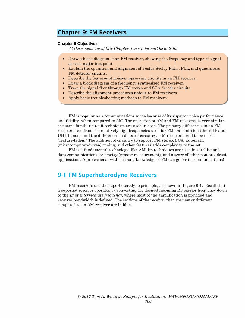
The oldest and least practical FM detector is the slope detector of Figure 9-3. This
detector relies on the frequency response of a tuned circuit. The slope detector works by utilizing the slope of a tuned circuit's frequency
response. It can be best understood as a two-step detector. First, the FM signal is converted into an AM signal, and then the resulting AM signal is envelope detected.
In Figure 9-3(a), the tuned circuit consists of transformer T1 and its internal capacitor, and the AM portion of the detector is built from D1, R1, and C1. This is in fact a standard AM detector circuit! In normal operation (AM detection), the input signal would be at the resonant frequency of the tank. In FM operation, the tank is deliberately mistuned, as shown in Figure 9-3(b).
No Need for AGC
Slope Detection
© 2017 Tom A. Wheeler. Sample for Evaluation. WWW.N0GSG.COM/ECFP 312
Detected OutputFM Input
T1D1
1N60
C10.01 uF
R14.7K
f
Resonant Frequency of Tank
Carrier Frequency
fc
fc + δ
fc - δ
Active Region
Second Possible Active Region
a) Slope Detector Circuit
b) Slope Detector Operation
Figure 9-3: The Slope Detector
By moving the tank frequency up, the carrier frequency now falls on the left-hand
slope of the tuned circuit's frequency response. As the carrier frequency increases, the amplitude of the tuned circuit output increases; as the carrier frequency decreases, the amplitude falls. The amplitude of the circuit's output depends on the frequency of the FM signal! By passing the resulting AM signal into the diode detector, the information is recovered.
The slope detector isn't an entirely practical FM detector for two reasons. First, this detector has a dual response. There are two points on the tuning curve of the tuned circuit that will provide a detected output. This will result in ambiguous tuning characteristics (a station will appear at two adjacent points on the tuning dial). Second, the shape of the tuned circuit's frequency response is not very linear, unless only a very small portion of the curve is used. For wideband FM detection, this would not work very well; the resulting carrier frequency swings are quite large (+/- 75 kHz), and considerable distortion of the sound would result.
The Foster-Seeley detector circuit is a vast improvement over the slope detector. It
provides a single response, and reasonably linear characteristics for wideband FM detection. This circuit can be best understood if developed in steps, as shown in Figure 9-4.
The Foster-Seeley
Detector

© 2017 Tom A. Wheeler. Sample for Evaluation. WWW.N0GSG.COM/ECFP 313
Va
Va
Vb
Vb
| Vac |
| Vbc |
T1
FM INPUT
REFERENCE FREQUENCY
Vc
T1
FM INPUT
REFERENCE FREQUENCY
Vc
C1
C1
D1
D2
R1
R2
C2RF BP
C3RF BP
FM INPUT
C2RF BP
C3RF BPD2
R2C1
T1
D1
R1
L1
C4
RF COUPLING
Vac
Vbc
AF OUTPUT = |Vac| - |Vbc|
AF OUTPUT = |Vac| - |Vbc|
a) Converting Frequency Changes to Phase Shifts
b) Summing the Magnitudes of Vac and Vbc Vectors
c) Eliminating the Reference Frequency Source
Figure 9-4: Development of the Foster-Seeley Detector
The operation of the Foster-Seeley detector is a two-step process, just like the slope
detector. Instead of converting input frequency changes to AM, the Foster-Seeley circuit converts the incoming FM signal into a series of phase shifts. The resulting signal, though not a true PM signal, is then phase-detected to produce a varying output voltage. The circuit can be developed in three steps.
Figure 9-4(a) shows the first step. The FM signal is coupled into transformer T1, whose secondary is parallel-resonated by C1 at the IF center frequency (usually 10.7 MHz). Capacitor C1 and the secondary inductance of T1 form a phase shifter circuit. A steady sine wave at the IF frequency of 10.7 MHz, voltage Vc, is applied to the center tap of T1.
© 2017 Tom A. Wheeler. Sample for Evaluation. WWW.N0GSG.COM/ECFP 314
Vc
Vb
Va
a) fin = fc : Vac = Vbc
Vac
Vbc
Vc
Vb
Va b) fin > fc : Vac > Vbc
Vac
Vbc
Vc
Vb
Va
c) fin < fc : Vac < Vbc
Vac
Vbc
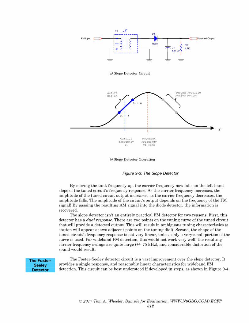
Figure 9-5: Phasor Relationships in the Foster-Seeley Detector
The phase shift produced at the secondary of T1 depends on the instantaneous
frequency of the FM signal being applied. At rest (f = fc ), the phase shift adjusted to be 90 degrees by tuning T1. The phasors appear as in Figure 9-5(a). Notice that the top output of the circuit is the phasor sum of the voltages Vc (the reference) and Va (the voltage from the top of T1). This voltage is Vac. The same happens at the bottom side of T1, and the voltage Vbc is developed here. Note the phase relationship between Va and Vb: They are 180 degrees out of phase. This is true due to the center-tap on the secondary of T1. When f = fc, the circuit is balanced. The outputs Vac and Vbc are equal in magnitude, and if their absolute values are subtracted, the result is zero.
What happens when the FM carrier frequency deviates upward? The phasor result is shown in Figure 9-5(b). Again, Va and Vb maintain their 180 degree relationship; they both

© 2017 Tom A. Wheeler. Sample for Evaluation. WWW.N0GSG.COM/ECFP 315
rotate in a counter-clockwise direction. Since Vc is the reference, it does not move. As you can see, the phasor results Vac and Vbc are now out of balance; Vac is much larger. To detect the out-of-balance condition, the circuit of 9-4b is used. Diodes D1 and D2 serve to rectify the AC voltages Vac and Vbc. The algebraic output of 9-4(b) is ( |Vac | - |Vbc | ).
Therefore, in Figure 9-4(b), when the input frequency rises, the rectified output Vac is larger than the |Vbc | output, and a positive output voltage results. The opposite effect occurs when the carrier frequency is lowered; now |Vbc | becomes larger, and the output voltage becomes negative. The circuit has effectively converted voltage into frequency.
The final refinement of the circuit is shown in Figure 9-4(c). The first two circuits require an oscillator to provide a reference frequency, and this oscillator must be phase-locked to the FM carrier signal. This is not very convenient, so the oscillator is replaced with a sample of the RF carrier voltage in Figure 9-4(c). The carrier voltage is coupled into the circuit through C4, and inductor L1 (which is usually adjustable) serves to allow an RF voltage drop to be developed to serve as the reference voltage.
Why does this work? The answer is that two rates of phase change occur in the circuit. The portion of the circuit containing L1 changes phase relatively slowly when the input frequency changes, because it contains only L1. The resonant circuit consisting of T1's secondary and C1 changes phase more quickly because it has two reactive parts (T1 and C1). Therefore, for practical purposes, the phase change across L1 is small enough to consider that portion of the circuit to have an approximately constant phase angle. The voltage across L1 is approximately a "reference" voltage.
The Foster-Seeley detector can reproduce a high-quality information signal, but has one limitation. In Figure 9-5, the size of the vectors Va and Vb determines the magnitude of voltage output from the detector. If the input voltage of the FM signal changes, these vectors will change in size, and the detector's output voltage will change accordingly. In other words, a Foster-Seeley detector doesn't reject AM. Since most noise is in the form of amplitude disturbances, it will pass through a Foster-Seeley detector and be reproduced in the audio. To prevent this, a limiter stage must precede a Foster-Seeley detector to prevent AM noise from reaching the circuit.
A modification to the Foster-Seeley circuit results in the ratio detector circuit of Figure 9-6. One thing most people notice immediately about this circuit is that "one of the diodes is in backwards!"
-Vbc
Vac
AF OUTPUT
D2
C3RF BP
D1
C2RF BP
C1
FM INPUT
C4
RF COUPLING
T1
L1
R1
R2
C5+
Figure 9-6: A Ratio Detector Circuit
The Ratio Detector

© 2017 Tom A. Wheeler. Sample for Evaluation. WWW.N0GSG.COM/ECFP 316
The operation of the ratio detector is very similar to that of the Foster-Seeley circuit. The difference involves how the audio output voltage is developed. Notice that the voltages Vac and -Vbc are developed on the top and bottom legs of the circuit, and that both of these voltages are ground referenced. The bottom voltage -Vbc appears as a negative value because D2 is reversed. Resistors R1 and R2 form a voltage divider. When the two voltages Vac and Vbc are equal, the output from the divider will be zero, since R1 and R2 are equal values. When Vac and Vbc become unequal, the voltage divider unbalances, and a positive or negative voltage output is produced, depending upon which voltage (Vac or Vbc) is larger, which in turn depends upon the input frequency.
In this manner, the operation is very similar to the Foster-Seeley circuit. The primary addition is capacitor C5, which sees the total voltage ( |Vac| + |Vbc| ). Even when the circuit unbalances, the sum of these two voltages is constant (when one gets smaller, the other becomes larger to compensate). Capacitor C5 is a large electrolytic, usually around 10 µF, and tends to stabilize the total voltage across the circuit. The benefit of capacitor C5 is that the circuit has a built-in limiting action, but only for short-term (less than a second or so) amplitude changes. The ratio detector does a better job of rejecting AM noise than the Foster-Seeley Circuit, but must still be preceded by a limiter amplifier circuit.
Vc
D2
C3RF BP
D1
C2RF BP
C1
T1
C5+
T2
FM INPUT
R1
R2
AF OUTPUT
Figure 9-7: A Very Common Form of the Ratio Detector
Figure 9-7 shows a very common form of the ratio detector that uses two adjustable
transformers. The operation is identical to Figure 9-6, except that the secondary of T2 is used to provide the reference voltage Vc. Usually T1 and T2 are a matched set of transformers designed especially for ratio detector duty, and may even be contained in one metal can (with the two screw adjustments visible).
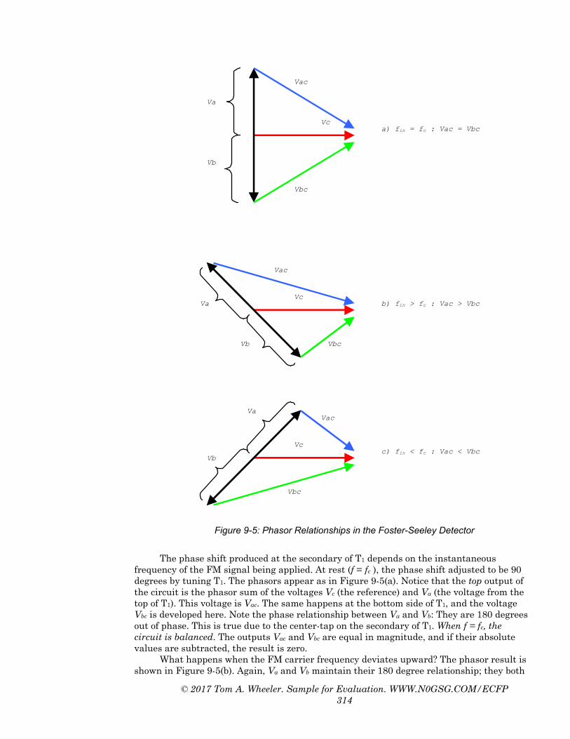
The Foster-Seeley and ratio detectors are excellent FM detectors, but require the use of bulky RF transformers. A phase-locked-loop, or PLL can be used as an FM detector by extracting the audio signal at the low-pass filter output, as shown in Figure 9-8.
PLL FM Detection
© 2017 Tom A. Wheeler. Sample for Evaluation. WWW.N0GSG.COM/ECFP 317
A
Loop Low Pass F i l te r VCO
Phase Detec tor
B
Y
A B C
D FM Input
Recovered Audio Output
Figure 9-8: The PLL FM Detector
The PLL FM detector looks too good to be true. How can such a simple circuit detect
FM? The answer comes from looking at the basic action of a phase locked loop. You might recall that the basic function of a PLL is to lock the VCO frequency exactly
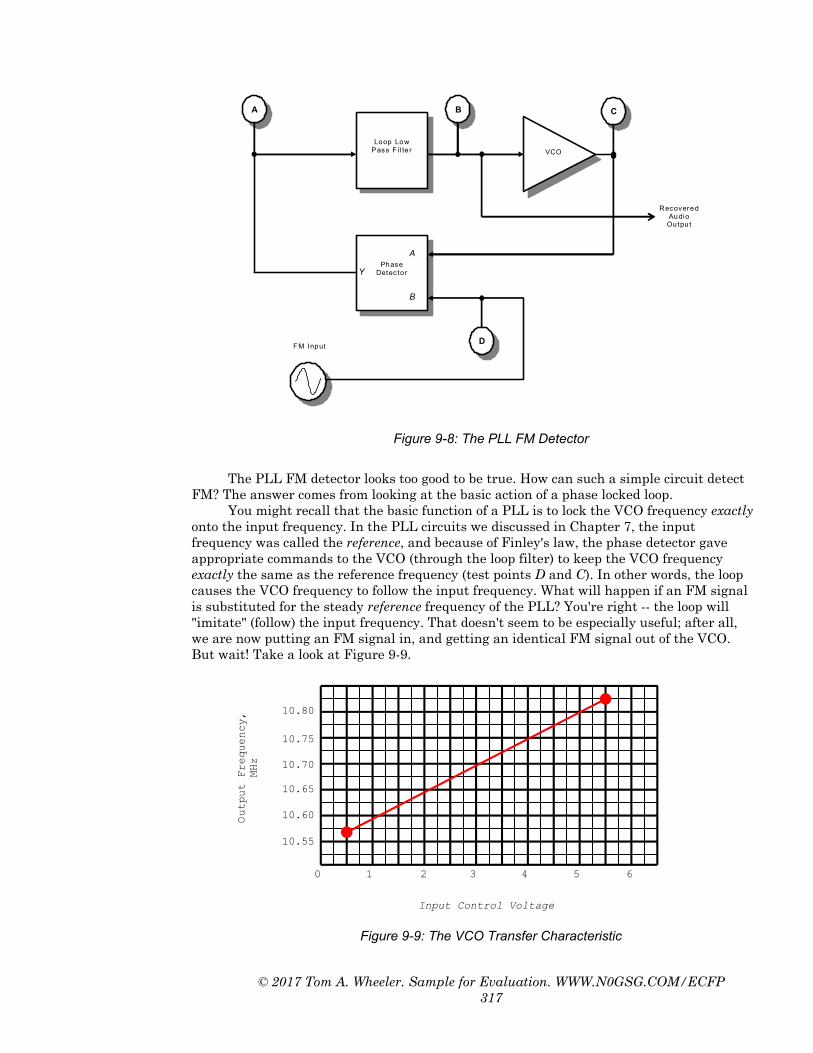
onto the input frequency. In the PLL circuits we discussed in Chapter 7, the input frequency was called the reference, and because of Finley's law, the phase detector gave appropriate commands to the VCO (through the loop filter) to keep the VCO frequency exactly the same as the reference frequency (test points D and C). In other words, the loop causes the VCO frequency to follow the input frequency. What will happen if an FM signal is substituted for the steady reference frequency of the PLL? You're right -- the loop will "imitate" (follow) the input frequency. That doesn't seem to be especially useful; after all, we are now putting an FM signal in, and getting an identical FM signal out of the VCO. But wait! Take a look at Figure 9-9.
Input Control Voltage
Output Frequency,
MHz
10.80
10.75
10.70
10.65
10.60
10.55
0 1 2 3 4 5 6
Figure 9-9: The VCO Transfer Characteristic

© 2017 Tom A. Wheeler. Sample for Evaluation. WWW.N0GSG.COM/ECFP 318
Figure 9-9 tells us that for the VCO frequency to change, its control voltage must change. The phase detector and low-pass filter in the loop will determine the correct control voltage for any applied input frequency. The "correct" voltage, of course, is the one that makes the VCO frequency exactly equal to the FM input frequency.
Suppose the input frequency is 10.7 MHz (the IF center frequency). What VCO control voltage will result? According to the graph in Figure 9-9, the VCO requires approximately 3 volts DC to produce 10.7 MHz out, so the DC control voltage will be 3 volts. An input of 10.7 MHz is converted to a DC voltage of 3 volts.
When the carrier frequency increases in a positive direction, the loop must follow. Suppose that an input frequency of 10.775 MHz (+75 kHz deviation) is applied. What VCO control voltage will result? Again, Figure 9-9 suggests that the VCO "needs" 4.5 volts for this to happen. An input of 10.775 MHz is converted to 4.5 volts.
Can you see what is happening? The loop must follow the input frequency changes. We're taking advantage of that behavior by "peeking" inside the loop to extract the DC control voltage for the VCO. The information signal will be riding on top of the DC control voltage; we simply block the DC with a capacitor to extract the information!
The PLL is an excellent FM detector, and can be built without any RF transformers at all. In fact, all of the circuitry can be built onto a chip. This makes it well suited for miniature circuitry. Since the input to the PLL is a digital input, it can be equipped with a Schmitt trigger, which provides automatic limiting action. The PLL can provide true limiting action on its own, without the addition of a limiter amplifier.
Figure 9-10 shows a PLL FM detector using the LM/NE565 PLL IC. This circuit is designed to operate on a carrier of 100 kHz, with nominal deviation of +/- 10 kHz. Variable resistor R106 sets the free-running frequency of the loop, which should be adjusted to 100 kHz (at pin 4 of the IC, the VCO output) with no signal applied to the FM INPUT. The LM565 IC contains the phase detector, VCO, and filter resistor. C105 and C106 are part of the loop RC filter circuit; R108 and C107 also act as part of the loop filter. R109, R110, C108, and C109 filter any 100 kHz RF signal from the detected FM output. C110 is a DC block, which leaves only the information signal at the AF OUT terminal.
Figure 9-10: A PLL FM Detector Utilizing the LM/NE565
V+ R TIN 1
IN 2
VCO OUT
PD VCO IN
V- C T
2
3
4
5
10 8
7
1 9
CTRLVLTG
NE565
VCO Free RunAdjustment
R 101
10R 10610K
R1071K
R109
10K
R110
10K
R10847K
C1010.1 uF
C1020.1 uF
C103
0.1 uF
C104470 pF
C10547 pF
C10647 pF
C107150 pF
C108.0022
C109.001 uF
C 110
10 uF
+
R102
4.7K
R103
4.7K
R10410K
R10510K
+15 V
FM INPUT
AF OUT

© 2017 Tom A. Wheeler. Sample for Evaluation. WWW.N0GSG.COM/ECFP 319
The quadrature detector of Figure 9-11 is a simple digital FM detector. It is perhaps
the simplest of the FM detectors; like the PLL, it provides built-in limiting action through a Schmitt-trigger input, and can be implemented on an IC chip.
AF OUTPUTFM Input
R1
L1
QUAD COIL
R2
C1
C2
+
Figure 9-11: The Quadrature Detector
The quadrature detector relies on conversion of frequency to phase shift, just like a
Foster-Seeley detector. In the quadrature detector above, the exclusive-OR gate functions as a phase detector. The FM input signal is applied directly to the top gate input, and indirectly to the bottom gate input through isolator resistor R1 and the quadrature coil, L1 (which usually contains a built-in capacitor to resonate at the IF center frequency).
R1 and L1 form a phase shifter network. As the FM input changes in frequency, the phase shift developed across R1, L1, and L1's internal capacitor varies. This causes the phase of the two signals at the phase-detector XOR gate to vary, which in turn causes the duty cycle of the pulses at the gate's output to vary. Figure 9-12 shows the phase-versus-output frequency relationship for the XOR phase detector.
Phase Difference, (B-A), Degrees
Output Duty Cycle,
%
100
80
60
40
20
0
0 45 90 135 180 225 270 315 360
Detector is adjusted for 90 degree shift @ fc
Figure 9-12: Output Voltage of the XOR Gate as a Function of Phase
The Quadrature
Detector

© 2017 Tom A. Wheeler. Sample for Evaluation. WWW.N0GSG.COM/ECFP 320
The varying duty-cycle output of the XOR gate is converted to a DC level by the filter comprised of R2 and C1. This DC level has the information riding on top of it. Capacitor C2 removes the DC level, leaving only recovered audio.
A quadrature detector is very easy to align. The technician simply applies the center frequency to the detector's input (usually 10.7 MHz) using an RF generator, and then monitors the DC voltage at the right hand portion of R2. The quadrature coil is adjusted until this voltage is one-half (50%) of Vcc; this provides a 90 degree phase shift between the two gate inputs (see Figure 9-12). This adjustment is necessary to provide a centered-Q point to allow both positive and negative frequency deviation. Alternately, the technician can insert the 10.7 MHz signal from the signal generator, and view the waveform at the XOR gate output pin with a scope. The quadrature coil is adjusted until a 50% duty cycle is obtained, which again signifies a 90 degree phase shift.
Some quadrature detectors require no alignment at all. It is possible to replace the parallel resonant circuit (L1 and its internal capacitor) with either a quartz crystal (in parallel resonant mode) or a ceramic resonator. This technique is commonly employed in narrowband communications-grade FM receivers.
Section Checkpoint
9-9 Explain how a slope detector works. What is the FM signal converted into before detection? 9-10 Give two reasons why the slope detector is not a very practical FM demodulator. 9-11 In a Foster-Seeley detector, what two voltages are equal when the input frequency is
equal to the center frequency? 9-12 What is the purpose of the diodes in a Foster-Seeley detector? 9-13 What two components are adjusted to align a Foster-Seeley detector? 9-14 What is the advantage of a ratio detector when compared to the Foster-Seeley circuit? 9-15 What is the purpose of capacitor C5 in Figure 9-6? 9-16 Explain how a PLL can be used to detect an FM signal. 9-17 How should R106 be adjusted in Figure 9-10? What does it set? 9-18 Explain how to align the quadrature detector of Figure 9-11.
9-3 A Complete FM Receiver
The circuit of a complete monaural FM receiver is shown in Figure 9-13. The receiver can also be viewed in block diagram form as Figure 9-1.
The FM receiver of Figure 9-13 is easiest to understand if analyzed one stage at a time. Let's follow each stage the incoming signal must take as it makes its way from the antenna to the loudspeaker.
The carrier signal from the rod antenna first enters the RF amplifier, Q4, after
entering the bandpass filter comprised of L3 and C15. (L3 and C15 are tuned to the center of the FM broadcast band. In a better quality unit, C15 would be tunable as a third ganged section of the tuning capacitor C17). You might notice that Q4 is a common base amplifier. Q4 has been drawn with the base electrode point down to emphasize this to the reader; this is a common convention in the world of RF. The common-base configuration gives much better high-frequency power gain than the common-emitter configuration.
The RF signal enters Q4's emitter through coupling capacitor C8, and leaves Q4's collector (in amplified form) and passes through the preselector bandpass filter. C17A (half of the tuning capacitor) and L2 form the preselector bandpass filter.
RF Amplifier
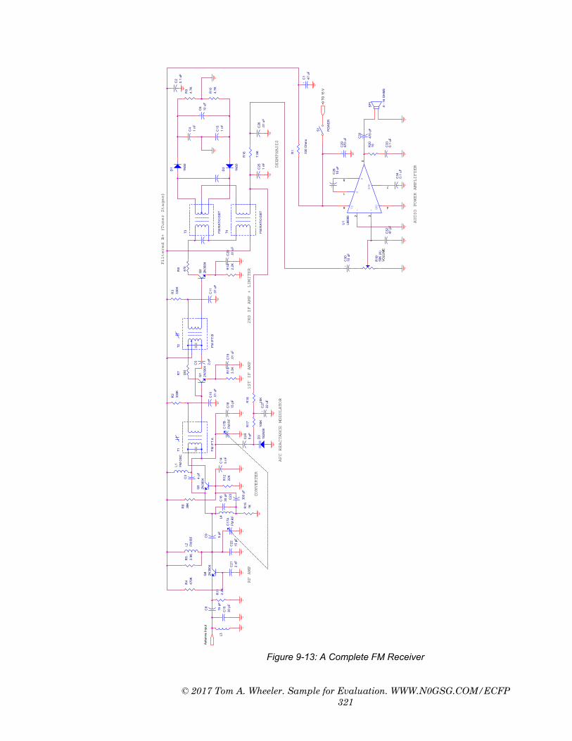
© 2017 Tom A. Wheeler. Sample for Evaluation. WWW.N0GSG.COM/ECFP 321
Figure 9-13: A Complete FM Receiver
AFC REACTANCE MODULATOR
RF AMP
CONVERTER
1ST IF AMP
2ND IF AMP + LIMITER
DEEMPHASIS
AUDIO POWER AMPLIFIER
Filtered B+ (Tuner Stages)
Q4
2N39
04
R4
470K
R11
2.2K
L3
L2 FM R
FR
53.
9K
C15
30 p
FC
212
nFC
2215
pF
C9
5 pF
C17
AFM
RF
C8
15 p
F
C24
5 pF
D3
1S26
38
R15
1K
C18
15 p
F
C16
30 p
F
T1 FM
IF
T A
R12
22K
R17
100K
R6
39K
C14
5 nF
R18
10K
C23
300
pF
L1 FM
OSC
L4
C3
4 pF
Q3
2N39
04Q
12N
3904
C27
22 u
F+
R13
3.3K
C19
.01
uF
T2 FM
IF
T B
R7
330
C5
2 pF
C11
.01
uF
Q2
2N39
04
R14
2.2K
C20
.01
uF
R8
470
D2
1N60
D1
1N60
C4
1 nF
C6
10 u
F+
T4 FM
RAT
IO D
ET
R9
4.7K
T3 FM
RAT
IO D
ET
R10
4.7K
C13
1 nF
C25
1 nF
R16
7.5K
C26
.01
uF
C2
0.1
uF
R1
330
Ohm
s
S1 POW
ER
SP1
4 - 1
6 O
HM
S
C34
0.1
uF
C30
10 u
F+
C32
47 p
F
C28
10 u
F
+
C29
470
uF+
C33
0.1
uF
C31
470
uF
+
R19
50K
(A)
VOLU
ME
R20
10
U1
LM38
6
- +
Vs
G
G
BYP
GND
2 3
6
1
8
5
7
4
C17
BFM
RF
C1
47 u
F+
C10
.01
uF
R2
330K
R3
330K
Ant
enna
Inpu
t
+9 T
O 1
5 V