Chapter 8

R t L T h iRoot Locus Techniques

Introduction

S t f d t bilit d t i d b l d l l

Typical closed-loop feedback control system

)1()( +ssG)3()( +

=ssH

System performance and stability determined by closed-loop poles

)2()(

+=

sssG

)4()(

+=

ssH

)3()1( ++ ssK sKGsT )()( =

Open-loop TF Closed-loop TF

)4()3(

)2()1()()(

++

++

=ss

sssKsHsKG

Zeros -1, -3 KsKsKsssKsHsKG

sT

3)48()6()4)(1(

)()(1)(

23 +++++++

=

+=

•Location of poles easily found•Variation of gain K do not affect the

•Location of poles need to factor the denominator difficult

•variation of gain K do change the location of

Poles 0, -2, -4

Easy way to know the CL pole locations w/o solving higher-order characteristic equation of CLTF for various gain K?

f g fflocation of any poles poles

various gain K?Root locus

• graphical representation of the closed-loop poles as a function of system parameters• Can be used to design system parameters of the high order systems to yield a desired system

specifications• Estimating closed-loop poles’ location when gain K is varied using open-loop poles• Represent the poles of T(s) as K varies

Vector representation of complex numbers

Vector Representation of Complex Numbers

Vector representation of complex numbers

Magnitude M and angle as θ∠Mθ

ωσ js +=Complex number

Magnitude M and angle , as θ∠Mθ

jF +++ )()()(Comple f nction hen ωσ js +)()(F ωσ jaassF ++=+= )()()(Complex function when ωσ js +=

Complex function F(s) has a zero at -a

)()( assF +=

)( as +a complex number can be represented by avector drawn from the zero of the function to thepoint s

)()(Ex) 25)7()(

jsssF

+→+=

Complicated functionm

)(

)()(

1

1

i

n

j

ii

ps

zssF

+∏

+∏=

=

= ∏ : productM: number of zerosN: number of poles

where

Value of F(s) at any point s

Each complex factor vector magnitude & angle

Magnitude of F(s)

i

n

j

i

m

i

ps

zs

lengthspolelengthszeroM

+∏

+∏=

∏∏

=

=

=

1

1

j=1

izs + Magnitude of the vector drawn from to the point s

ips + Magnitude of the vector drawn from to the point sipiz

whereip g p

Angle of F(s) at any point s ∑∑ −=nm

polestoangleszerostoanglesθ

∑∑==

+∠−+∠=n

ji

m

ii pszs

11)()(

Measured from the positive real axispositive real axis

Ex) Find F(s) at the point s = -3 + j4

)2()1()(

++

=ssssF Magnitude

217.017520

414342

21

==+−+−

+−=

++

=∏∏

=jj

jss

slengthpolelengthzeroM

ooo 010491266116

)( −=∠ ∑∑ polestoangleszerostoanglessF

θθθ

Angle

o

ooo

3.114

0.1049.1266.116201

−=

−−=−−= −==−= ppz θθθ

oo 6.11642tan90 1 =⎟⎠⎞

⎜⎝⎛+ −

4 ⎠⎝

444 111 ⎟⎞

⎜⎛

⎟⎞

⎜⎛

⎟⎞

⎜⎛

or

o34.1141

4tan3

4tan2

4tan)( 111 −=⎟⎠⎞

⎜⎝⎛−

−⎟⎠⎞

⎜⎝⎛−

−⎟⎠⎞

⎜⎝⎛−

=∠ −−−sF

Subject tracking camera system

Properties of Root LocusKnob에해당

Subject tracking camera system

Equivalent closed loop TF Closed loop poles function of gain K

241010 2

2,1KP −±−

=

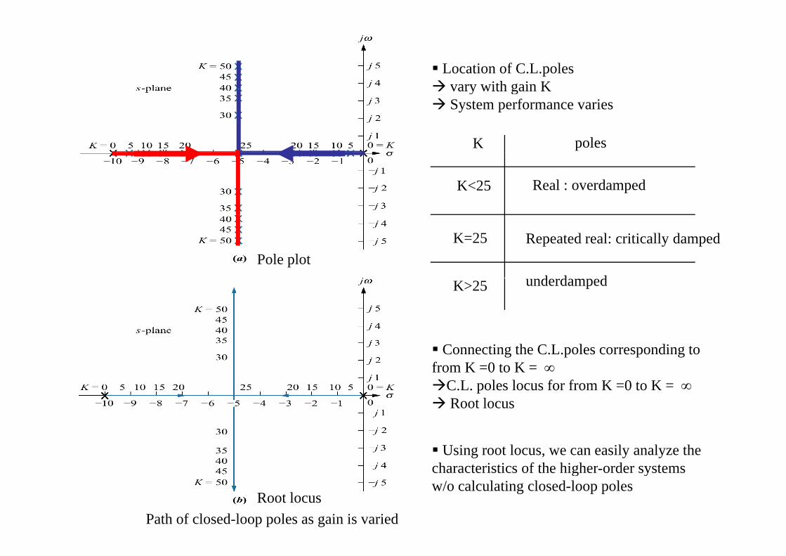
Location of C.L.polesvary with gain K

polesK

vary with gain KSystem performance varies

K<25 Real : overdamped

Pole plotK=25 Repeated real: critically damped

d d dK>25 underdamped

Connecting the C.L.poles corresponding to from K =0 to K = ∞

C.L. poles locus for from K =0 to K = ∞Root locusRoot locus

Using root locus, we can easily analyze the characteristics of the higher order systems

Root locusPath of closed-loop poles as gain is varied

characteristics of the higher-order systems w/o calculating closed-loop poles

Properties of Root Locus

Higher-order systems difficult to calculate the closed-loop pole location for various gain K’s.Using root locus, without solving denominator polynomial of closed loop TF, it is possible to

have rapid sketch of closed-loop poles location change for various gain K’s(root locus)

)()(1)()(

sHsKGsKGsT

+=C.L.T.F.

(root locus)

)()(1 sHsKG+

Characteristic equation (i.e. C.L. poles = the values that satisfy the characteristic equation

0)()(1 =+ sHsKGo180)12(11)()( +∠=−= ksHsKG L,3,2,1,0 ±±±=k

o180)12()()(∠ kHKG

1)()( =sHsKG

o180)12()()( +=∠ ksHsKG

1Any complex number s that

f h d)()(

1sHsG

K =

Angle condition ⇒ determines the root locus

satisfies these conditions⇒ closed-loop poles!

Angle condition ⇒ determines the root locusMagnitude condition ⇒ Determines the specific position corresponding to

specific value of K on the root locus

Ex)

)4)(3()()( ++=

ssKsHsKG )4)(3()( ssKsT ++=

Open-loop TF Closed-loop TF

)2)(1()()(

++=

sssHsKG

)122()73()1()( 2 KsKsK

sT+++++

=

jbIf a pole is a closed-loop pole for some value of gain K

t ti f djbas +=

)()(o180)12()()(∠ kHKGjbas += must satisfy and

Consider as the first test point 321 js +−=

1)()( =sHsKGo180)12()()( +=∠ ksHsKG

)()(∠ ∑∑ ltltlHKG

321 js +−=

o

oooo

55.70

43.1089057.7131.56

)()(

4321

11

−=

−−+=−−+=

−=∠ ∑∑θθθθ

polestoangleszerostoanglessHsKG

o180≠321 js +−= is not a closed-loop pole

What about )2/2(22 js +−= o180)()( 22 =∠ sHsKG

is a closed-loop pole for some value of gain K2

)2/2(22 js +−=

33.0)12.2)(22.1(

22)22.1(

2/222/21

2/22/21

4321

)()(1

22

22

22

==++

+−=

++++

=∏∏

==jj

jj

ssss

lengthzerolengthpole

sHsGK

is a closed-loop pole (i.e. is a point on the root locus) when K= 0.33)2/2(22 js +−=

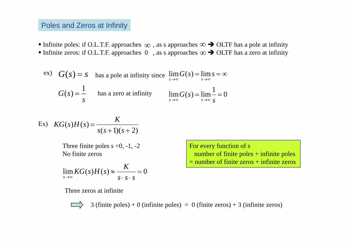
Poles and Zeros at Infinity

Infinite poles: if O.L.T.F. approaches , as s approaches OLTF has a pole at infinityInfinite zeros: if O.L.T.F. approaches 0 , as s approaches OLTF has a zero at infinity

∞ ∞∞

ssG =)(

sG 1)( =

has a pole at infinity since

has a zero at infinity

∞==∞→∞→

ssGsslim)(lim

01lim)(lim ==sG

ex)

ssG )( y

)()( KsHsKG

0lim)(lim ==∞→∞→ s

sGss

Ex)

For every function of sb f fi i l i fi i l

)2)(1()()(

++=

ssssHsKG

Three finite poles s =0, -1, -2N fi i

Ex)

number of finite poles + infinite poles = number of finite zeros + infinite zeros

No finite zeros

0)()(lim =⋅⋅

≈∞→ sss

KsHsKGs sss

Three zeros at infinite

3 (finite poles) + 0 (infinite poles) = 0 (finite zeros) + 3 (infinite zeros)( p ) ( p ) ( ) ( )

Sketching the Root Locus

1 Mark open loop poles with x’s and open loop zeros with o’sK=0~ 변할때 root locus가어떻게변하는지본다.∞

Shows how location of the CL poles move as K varies from 0 to ∞

1. Mark open loop poles with x s and open loop zeros with o s

K>0일때, 실수축상에서 Test point의오른쪽에있는 pole과 zero의수의합이홀수이면2. Draw root loci on the real-axis to the left of an odd number of real poles plus zeros

그점은 root loucs상에있다

3 Root locusstarts at (finite and infinite) open-loop poles

and

(i.e. K = 0)o180)12()()( +=∠ ksHsKGSatisfying the angle condition

3. Root locus

4 Draw the asymptote of root locus

andends at (finite and infinite) open-loop zeros

(i.e. K = )∞4. Draw the asymptote of root locus

a. Real-axis intercept or center of asymptote

zerosfinitepolesfinite −= ∑∑σ

zerosfinitepolesfinitea ## −σ

k 180)12( +=

o

θ 3210 ±±±=kb. 양의실수축과이루는각도

Note.Number of branches of the root locus = number of closed loop poles = system order

zerosfinitepolesfinitea ## −θ 3,2,1,0 ±±±k

- Number of branches of the root locus = number of closed-loop poles = system order(Branch: path that one pole traverse)

- The root locus is symmetrical about the real axis

)4)(3()()( ++=

ssKsHsKG

Open-loop TF

)2)(1()()(

++=

sssHsKG

Root locus starts at -1 and -2 meet between -1 and -2meet between -1 and -2break out into complex planereturn to real axis somewhere between -3 and -4ends at -3 and -4ends at 3 and 4

ex 8.2)Ends at zero t i fi it

1 Mark OL poles and zeros

at infinity

1. Mark OL poles and zeros2. Draw loci on real axis to the left of odd number3. Start at poles and end at zeros4. Draw asymptote

34

14)3()4210(

−=−−−−−

=aσ314 −

##180)12(

−+

=zerosfinitepolesfinite

kaθ

o 3/ππ

23/5103/

======

kforkforkfor

πππ

3/5π

Ends at zero at infinity

23/5 == kforπ

# of asymptotes = # finite poles - #finite zeros = 3# f b h # f CL l d 4# of branches = # of CL poles = system order = 4

Ends at zero at infinity

The root locus is symmetrical about the real axisCheck!

# infinite zeros (3) + #finite zero (1) = #finite poles (4)

Refining the Sketch(breakaway from real axis and move into the complex plane)

A. Real-axis Breakaway and Break-in Point

1σ−

2σ: Breakaway point: Break-in Point

As K increases2

Break-in and Breakaway angle :n

o180

n: # of CL poles arriving at or departing fromn: # of CL poles arriving at or departing from the BA or BI on the real axis

Two poles 90o at BATwo zeros 90o at BITwo zeros 90 at BI

Determine the location of BA and BI pointOn the real axis between open-loop poles, gain K is maximum at BA pointp p p g pOn the real axis between open-loop zeros, gain K is minimum at BI point

0=ddK

1

=σsds

σ is an either BA or BI point where

0)()(1 =+ sHsKGQ)()(1

sHsGK −= ( )

where

Characteristic equation

Ex))23(

)158()2)(1()5)(3()()( 2

2

+++−

=++−−

=ssssK

ssssKsHsKG

)())((

)158()23(

2

2

+++

−=ssssK

)158( +− ss

)82)(23()158)(32( 22 ++++ ssssssdK

)612611(

)158()82)(23()158)(32(

2

22

−−

+−−++−+−+

−===

σσσσ ss ss

ssssssdsdK

823451

0)158(

)612611(22 =

+−=

σσσσ

A d i82.3,45.1−=σ BA and BI point

B. j -Axis Crossingsω

A point on the root locus that separates the stable operation of the system from the

bl iunstable operation

A pole on j -axis at a certain gain KωA pole on j axis at a certain gain Kω

How to find the value of and K?ω

Method I) Substitute s = j directly into characteristic equationω

ωσ js +=(A pole on j -axisω0

)

Method II) Use Routh table A row of entire zeros of Routh table pole on j -axis possible ω

Ex) find the frequency and gain K for which the root locus crosses the imaginary axis.

KsKssssKsT

3)8(147)3()( 234 +++++

+=

C.L.T.F.

Method I) Characteristic equation:

)(

Method I)03)8(147 234 =+++++ KsKsss

q

S b tit t j i t h t i ti tiωAs j is a pole of closed-loop system, it must satisfy characteristic equationω

03))(8()(14)(7)( 234 =+++++ KjKjjj ωωωω

234

Substitute s = j into characteristic equationω

03))(8(147 234 =+++−− KjKj ωωωω

0314 24 =+− KωωReal part

0)8(7 3 =++− ωω KImaginary part

Solve for and Kω59.1±=ω

65.9=KRoot locus crosses j -axis at at a gain of

ω 59.1js ±=65.9=K

Method II) Use Routh tableKsKsss

sKsT3)8(147

)3()( 234 ++++++

=

No sign changes from s4 to s2

2 LHP l2 LHP poles2 remaining, but even polynomials of s2

requires symmetric poles2 poles should be on j -axis ω

Only s1 row can make all zero row 0720652 =+−− KK

p jω

65.9=KAssuming K>0, then

Form even polynomial using s2 row22 07.20235.8021)90( 22 =+=+− sKsK

59.1js ±=59.1j65.9=K

Root locus crosses j -axis at at a gain of

6590 <≤ KSystem is stable for

ω 59.1js ±=

59.1j−65.9=K

0=K0=K65.9=K

65.90 <≤ KSystem is stable for 59.1j65.9K

C. Angles of Departure and Arrival

Root locus starts at open-loop poles (ex. p1) and ends at finite and infinite open-loop zeros (ex. z2)For more accurate root locus, need to know the root locus departure angle from the complex poles

arrival angle to the complex zeros

If a complex number s1 is on root-locus and close ( ) to a complex pole p1, i.e. is one of the closed-loop poles, it must satisfy angle condition

ε

11

180)12(

)()(

+=

−=∠ ∑∑ok

polestoangleszerostoanglessHsKG

Test point

z2

541362

)(θθθθθθ −−−++=

ps1p1

if t t k th d t l f l lif want to know the departure angle from a complex pole p1

o180)12(543621 +−−−++= kθθθθθθ

C. Angles of Departure and Arrival

Root locus starts at open-loop poles (ex. p1) and ends at finite and infinite open-loop zeros (ex. z2)For more accurate root locus, need to know the root locus departure angle from the complex poles

arrival angle to the complex zeros

If a complex number s1 is on root-locus and close ( ) to a complex pole p1, i.e. is one of the closed-loop poles, it must satisfy angle condition

ε

11

180)12(

)()(

+=

−=∠ ∑∑ok

polestoangleszerostoanglessHsKGTest point

s1

541362

)(θθθθθθ −−−++=

if t t k th d t l f l l

1

if want to know the departure angle from a complex pole p1

o180)12(543621 +−−−++= kθθθθθθ

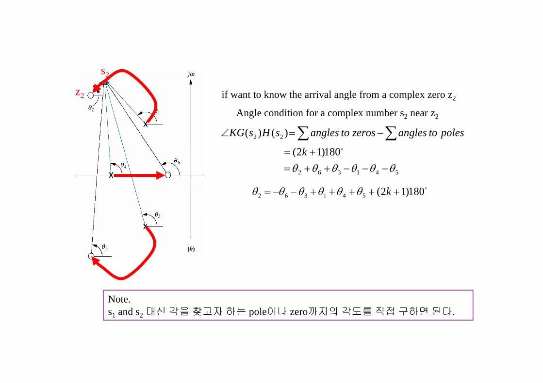
if want to know the arrival angle from a complex zero z2z2

s2

Angle condition for a complex number s2 near z2

22

180)12(

)()( −=∠ ∑∑ok

polestoangleszerostoanglessHsKG

o180)12( +++++= kθθθθθθ

541362

180)12(θθθθθθ −−−++=

+= ok

180)12(541362 +++++−−= kθθθθθθ

Note. s1 and s2대신각을찾고자하는 pole이나 zero까지의각도를직접구하면된다.

Ex) find the angle of departure from the complex poles and sketch the root locus

Open loop poles at -3, -1±j1

Departure angle from -1+j1

o180)12(4213 +=−−− kθθθθ

oo

o

1801tan901tan

180)12(

11

4231

⎟⎞

⎜⎛

⎟⎞

⎜⎛

+−−−=

−−

kθθθθ

o

o

41086.251

1802

tan901

tan

−=

−⎟⎠

⎜⎝

−−⎟⎠

⎜⎝

=

4.108=

D. Plotting and Calibrating the Root Locus

How to find exact point at which root locus satisfies certain conditions and the gain at that point?How to find exact point at which root locus satisfies certain conditions and the gain at that point?

Ex) Find exact point at which root locus crosses the 0.45 damping line and the gain at that point)3(K

Method I)

)4)(2)(1()3()()(+++

+=

sssssKsHsKG

θζ cos=

θ

θζ cos=

o25.63)45.0(cos 1 == −θ

On the line only a point with radius r = 0 747 satisfies angle condition450ζOn the line, only a point with radius r = 0.747 satisfies angle conditiono180)12()()( +=∠ ksHsKG

54312 θθθθθ −−−−=

45.0=ζ

lengthspolelengthszerosHsG

ps

zssHsG

i

n

j

i

m

i

∏∏

=⇒+∏

+∏=

=

= )()()(

)()()(

1

1

At that point, the corresponding gain 71.1)()(

1==

∏∏

==B

EDCAlengthzerolengthpole

sHsGK

Ex) Find exact point at which root locus crosses the 0.358 damping line and the gain at that pointMethod II)

)6)(4)(1(1)(

+++=

ssssG

2222

23

))((1

))((1

124101

)(1)(

)()(

ssssGsG

sRsC

ζ==

+++=

+=

2223

2222

)716.0()716.0(1

)716.0)(()2)((

nnnn

nnnn

sss

ssssss

αωωαωαω

ωωαωζωα

+++++=

++++++

o02.69)358.0(cos 1 == −θ

3580=ζ

⎪

⎪⎨

⎧

=+

=+

24716.0

10716.02nn

n

ωαω

αω8133.2=nω

3580=ζ 627200721 js ±=

358.0ζ

⎪⎩ =12

nαω358.0=ζ

CL pole pair on =0.358 damping lineζ180 69 02o

627.20072.1 jsd ±−=

θθABC

627.20072.11 2 jjs nn ±−=−±−= ζωζω ×××180-69.02o

-4 -1 0-6×

1θ2θ3θ

o180321 =−−− θθθCBAlengthzerolengthpole

sHsGK =

∏∏

==)()(

1

Comments

To be stableTo be stable⇒All C.L. poles must be in LHP

If#O.L. poles - #finite zeros ⇒ There is a vlue of the gain K beyond

3≥which root roci enter the RHP(i..e system becomes unstable)

Nonminimum-Phase SystemsSkip!

Minimum phase system: all the poles and zeros lie in LHP

Nonminimum phase system: at least one pole or zero lies in RHPNonminimum phase system: at least one pole or zero lies in RHP

)1()1()(

+−

=Tss

sTKsG a0&1)( >= aTsH)1( +Tss )( a

)1()1()(

+−

−∠=∠Tss

sTKsG a Phase shift ⇒ this is why it is called nonminimum phase

)12(180

180)1()1()(

o

o

+±=

++−

∠=

kTss

sTK a oo 02180)1()1(

=⋅±=+−

∠ kTss

sTK a

)12(180 +±= k

Locus Not on here!

Generalized Root Locus

So far, root locus as a function of the forward-path gain KHow to draw root locus for variations of other parameters? Ex) root locus for variations of the value of open loop pole p1?

10))(2(

10)()(1pss

sHsKG++

= gain K was a multiplying factor of the function but P1 is not.

Denominator of C.L.T.F. for a root locus for gain K variation )()(1 sHsKG+g

10)()( ==sKGsT

)()(1 1 sHsGp+

)()(

For a root locus for p1 variation, we need a CLTF denominator

)2(10210

102)2()()(1)(

12

112

++++=

++++=

+=

spss

pspssHsKGsT

Isolating p1 )2(102 1 ++++ spss

)2(102

102

+++= sp

ss

102)2(1 2

1

+++

+ss

sp

102)2()()( 2

1

+++

=ss

spsHsKGPath of closed loop poles

P1 is now a multiplying factor of the open loop transfer function

102)2()()( 2 ++

+=

ssssHsG

Path of closed loop poles as p1 is increased

Summary of the Steps for Constructing Root Loci

1. Convert into a form in which system parameter is a multiplying factor2. Locate the open-loop poles and zeros on the s-plane3. The branches start from open-loop poles and end at finite or infinite zerosp p p4. Draw the root locus on the real axis5. Determine the asymptotes of root locus6. Find the breakaway and break-in points7 D t i th l f d t / i l f /t l l /7. Determine the angle of departure/arrival from/to a complex pole/zero8. Find the points where the root loci may cross the imaginary axis9. Locate the closed-loop poles on the root locus and determine the corresponding gain K by

use of the magnitude conditiong

Root Locus for Positive-Feedback System

)()()()( sKGsT =

)()(1)(

sHsKG−

Positive feedback system

0)()(1 =− sHsKGA closed-loop pole s exist when

ksHsKG o36011)()( ∠== 3,2,1,0 ±±±=k

Angle condition for a root locus of positive feedback system kHKG o360)()(Angle condition for a root locus of positive feedback system ksHsKG 360)()( =

Rules for sketching root locusRead by yourself…