chapter 8 · chapter 8 halocarbon scenarios, ozone depletion potentials, and global warming...
TRANSCRIPT
CHAPTER 8Halocarbon Scenarios, Ozone Depletion
Potentials, and Global Warming Potentials
Lead Authors:J.S. Daniel
G.J.M. Velders
Coauthors:A.R. DouglassP.M.D. Forster
D.A. HauglustaineI.S.A. Isaksen
L.J.M. KuijpersA. McCulloch
T.J. Wallington
Contributors:P. Ashford
S.A. MontzkaP.A. NewmanD.W. Waugh
Final Release: February 2007From Scientific Assessment of Ozone Depletion: 2006

CHAPTER 8
HALOCARBON SCENARIOS, OZONE DEPLETION POTENTIALS,AND GLOBAL WARMING POTENTIALS
Contents
SCIENTIFIC SUMMARY . . . . . . . . . . . . . . . . . . . . . . . . . . . . . . . . . . . . . . . . . . . . . . . . . . . . . . . . . . . . . . . . . . . . . 8.1
8.1 INTRODUCTION . . . . . . . . . . . . . . . . . . . . . . . . . . . . . . . . . . . . . . . . . . . . . . . . . . . . . . . . . . . . . . . . . . . . . . . 8.5
8.2 HALOCARBON LIFETIMES, OZONE DEPLETION POTENTIALS, AND GLOBALWARMING POTENTIALS . . . . . . . . . . . . . . . . . . . . . . . . . . . . . . . . . . . . . . . . . . . . . . . . . . . . . . . . . . . . . . . . 8.5
8.2.1 Introduction . . . . . . . . . . . . . . . . . . . . . . . . . . . . . . . . . . . . . . . . . . . . . . . . . . . . . . . . . . . . . . . . . . . . . 8.58.2.2 Ozone Depletion Potentials . . . . . . . . . . . . . . . . . . . . . . . . . . . . . . . . . . . . . . . . . . . . . . . . . . . . . . . . . 8.5
8.2.2.1 Atmospheric Lifetimes . . . . . . . . . . . . . . . . . . . . . . . . . . . . . . . . . . . . . . . . . . . . . . . . . . . . . . 8.68.2.2.2 Fractional Release Factors . . . . . . . . . . . . . . . . . . . . . . . . . . . . . . . . . . . . . . . . . . . . . . . . . . . 8.68.2.2.3 Ozone Destruction Effectiveness . . . . . . . . . . . . . . . . . . . . . . . . . . . . . . . . . . . . . . . . . . . . . . 8.78.2.2.4 ODP Values . . . . . . . . . . . . . . . . . . . . . . . . . . . . . . . . . . . . . . . . . . . . . . . . . . . . . . . . . . . . . . 8.8
8.2.3 Direct Global Warming Potentials . . . . . . . . . . . . . . . . . . . . . . . . . . . . . . . . . . . . . . . . . . . . . . . . . . . . 8.88.2.4 Degradation Products and Their Implications for ODPs and GWPs . . . . . . . . . . . . . . . . . . . . . . . . . 8.13
8.3 FUTURE HALOCARBON SOURCE GAS CONCENTRATIONS . . . . . . . . . . . . . . . . . . . . . . . . . . . . . . . . .8.138.3.1 Introduction . . . . . . . . . . . . . . . . . . . . . . . . . . . . . . . . . . . . . . . . . . . . . . . . . . . . . . . . . . . . . . . . . . . . 8.138.3.2 Baseline Scenario (A1) . . . . . . . . . . . . . . . . . . . . . . . . . . . . . . . . . . . . . . . . . . . . . . . . . . . . . . . . . . . . 8.15
8.3.2.1 Emissions . . . . . . . . . . . . . . . . . . . . . . . . . . . . . . . . . . . . . . . . . . . . . . . . . . . . . . . . . . . . . . . 8.158.3.2.2 Mixing Ratios . . . . . . . . . . . . . . . . . . . . . . . . . . . . . . . . . . . . . . . . . . . . . . . . . . . . . . . . . . . . 8.218.3.2.3 Equivalent Effective Stratospheric Chlorine . . . . . . . . . . . . . . . . . . . . . . . . . . . . . . . . . . . . 8.25
8.3.3 Alternative Projections . . . . . . . . . . . . . . . . . . . . . . . . . . . . . . . . . . . . . . . . . . . . . . . . . . . . . . . . . . . . 8.288.3.3.1 Emissions . . . . . . . . . . . . . . . . . . . . . . . . . . . . . . . . . . . . . . . . . . . . . . . . . . . . . . . . . . . . . . . 8.288.3.3.2 Mixing Ratios . . . . . . . . . . . . . . . . . . . . . . . . . . . . . . . . . . . . . . . . . . . . . . . . . . . . . . . . . . . . 8.288.3.3.3 Equivalent Effective Stratospheric Chlorine . . . . . . . . . . . . . . . . . . . . . . . . . . . . . . . . . . . . 8.30
8.3.4 Uncertainties in ODS Projections . . . . . . . . . . . . . . . . . . . . . . . . . . . . . . . . . . . . . . . . . . . . . . . . . . . . 8.32
8.4 OTHER PROCESSES RELEVANT TO FUTURE OZONE EVOLUTION . . . . . . . . . . . . . . . . . . . . . . . . . . 8.34
8.5 INDIRECT GWPS . . . . . . . . . . . . . . . . . . . . . . . . . . . . . . . . . . . . . . . . . . . . . . . . . . . . . . . . . . . . . . . . . . . . . . 8.35
REFERENCES . . . . . . . . . . . . . . . . . . . . . . . . . . . . . . . . . . . . . . . . . . . . . . . . . . . . . . . . . . . . . . . . . . . . . . . . . . . . . 8.36

HALOCARBON SCENARIOS, ODPs, AND GWPs
8.1
SCIENTIFIC SUMMARY
Ozone Depletion Potentials and Global Warming Potentials
• The effectiveness of bromine compared with chlorine on a per-atom basis for global ozone depletion, typi-cally referred to as αα , has been re-evaluated upward from 45 to a value of 60. The calculated values from threeindependent two-dimensional models range between 57 and 73, depending on the model used and depending on theassumed amount of additional bromine added to the stratosphere by very short-lived substances (VSLS).
• Semi-empirical Ozone Depletion Potentials (ODPs) have been re-evaluated, with the most significant changebeing a 33% increase for bromocarbons due to the update in the estimate for the value of αα . A calculationerror in the previous Assessment, which led to a 13% overestimate in the halon-1211 ODP, has been corrected.
• Direct Global Warming Potentials (GWPs) have been updated to account for revised radiative efficiencies(HFC-134a, carbon tetrafluoride (CF4), HFC-23, HFC-32, HFC-227ea, and nitrogen trifluoride (NF3)) andrevised lifetimes (trifluoromethylsulfurhexafluoride (SF5CF3) and methyl chloride (CH3Cl)). In addition, thedirect GWPs for all compounds have been affected by slight decreases in the carbon dioxide (CO2) absolute GlobalWarming Potentials for various time horizons.
• Indirect GWPs have been updated primarily to reflect the later return of ozone-depleting substances (ODSs)to 1980 levels estimated in this Assessment and to account for the increased bromine efficiency factor. Directand indirect GWPs are presented separately due to concern over the appropriateness of combining them into netGWPs for application in certain climate change issues.
Projections of Halocarbon Abundances and Implications for Policy Formulation
• Several of the options evaluated for accelerating the future reduction of ODS abundances demonstrategreater effectiveness than assessed previously. These options are assessed using equivalent effective strato-spheric chlorine (EESC) derived from projections of the atmospheric abundances of ODSs based on historic emis-sions, observations of concentrations, reported production, estimates of future production, and newly availableestimates of the quantities of ODSs present in products in 2002 and 2015.
• The date when EESC relevant to midlatitude ozone depletion returns to pre-1980 levels is 2049 for the base-line (A1) scenario, about 5 years later than projected in the previous Assessment. This later return is prima-rily due to higher estimated future emissions of CFC-11, CFC-12, and HCFC-22. The increase in CFC emissionsis due to larger estimated current bank sizes, while the increase in HCFC-22 emissions is due to larger estimatedfuture production.
• For the polar vortex regions, the return of EESC to pre-1980 conditions is projected to occur around 2065,more than 15 years later than the return of midlatitude EESC to pre-1980 abundances. This later return isdue to the older age of air in the lower stratosphere inside the polar vortex regions. This metric for the polar vortexregions has not been presented in previous ozone Assessments.
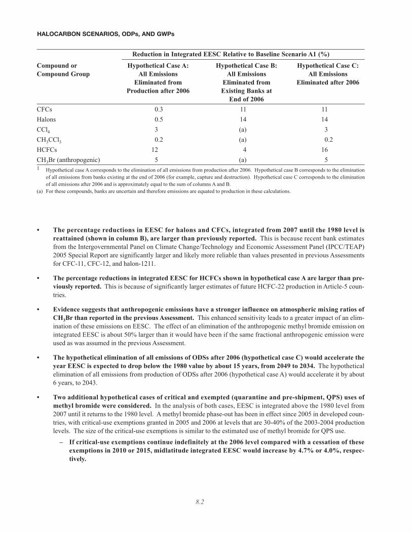
• Three classes of hypothetical cases are presented here to illustrate the maximum potential for reducing mid-latitude EESC if anthropogenic production or emission were eliminated after 2006 and if the existing banksat the end of 2006 were fully eliminated. The sizes of the banks considered for elimination are equal to the totalestimated production through 2006 minus all estimated emissions through 2006. These cases are not mutuallyexclusive, and separate effects of the elimination of production, emissions, and banks are not additive.
The table below shows the percentage reductions in integrated EESC relative to the baseline (A1) scenario that canbe achieved in these hypothetical cases (see table footnote 1). EESC is integrated above the 1980 level from 2007until it returns to the 1980 level (about 2050), and any potential contribution from VSLSs is neglected.
8.2
• The percentage reductions in EESC for halons and CFCs, integrated from 2007 until the 1980 level isreattained (shown in column B), are larger than previously reported. This is because recent bank estimatesfrom the Intergovernmental Panel on Climate Change/Technology and Economic Assessment Panel (IPCC/TEAP)2005 Special Report are significantly larger and likely more reliable than values presented in previous Assessmentsfor CFC-11, CFC-12, and halon-1211.
• The percentage reductions in integrated EESC for HCFCs shown in hypothetical case A are larger than pre-viously reported. This is because of significantly larger estimates of future HCFC-22 production in Article-5 coun-tries.
• Evidence suggests that anthropogenic emissions have a stronger influence on atmospheric mixing ratios ofCH3Br than reported in the previous Assessment. This enhanced sensitivity leads to a greater impact of an elim-ination of these emissions on EESC. The effect of an elimination of the anthropogenic methyl bromide emission onintegrated EESC is about 50% larger than it would have been if the same fractional anthropogenic emission wereused as was assumed in the previous Assessment.
• The hypothetical elimination of all emissions of ODSs after 2006 (hypothetical case C) would accelerate theyear EESC is expected to drop below the 1980 value by about 15 years, from 2049 to 2034. The hypotheticalelimination of all emissions from production of ODSs after 2006 (hypothetical case A) would accelerate it by about6 years, to 2043.
• Two additional hypothetical cases of critical and exempted (quarantine and pre-shipment, QPS) uses ofmethyl bromide were considered. In the analysis of both cases, EESC is integrated above the 1980 level from2007 until it returns to the 1980 level. A methyl bromide phase-out has been in effect since 2005 in developed coun-tries, with critical-use exemptions granted in 2005 and 2006 at levels that are 30-40% of the 2003-2004 productionlevels. The size of the critical-use exemptions is similar to the estimated use of methyl bromide for QPS use.
– If critical-use exemptions continue indefinitely at the 2006 level compared with a cessation of theseexemptions in 2010 or 2015, midlatitude integrated EESC would increase by 4.7% or 4.0%, respec-tively.
Reduction in Integrated EESC Relative to Baseline Scenario A1 (%)
Compound or Hypothetical Case A: Hypothetical Case B: Hypothetical Case C:Compound Group All Emissions All Emissions All Emissions
Eliminated from Eliminated from Eliminated after 2006Production after 2006 Existing Banks at
End of 2006CFCs 0.3 11 11Halons 0.5 14 14CCl4 3 (a) 3CH3CCl3 0.2 (a) 0.2HCFCs 12 4 16CH3Br (anthropogenic) 5 (a) 51 Hypothetical case A corresponds to the elimination of all emissions from production after 2006. Hypothetical case B corresponds to the elimination
of all emissions from banks existing at the end of 2006 (for example, capture and destruction). Hypothetical case C corresponds to the eliminationof all emissions after 2006 and is approximately equal to the sum of columns A and B.
(a) For these compounds, banks are uncertain and therefore emissions are equated to production in these calculations.
HALOCARBON SCENARIOS, ODPs, AND GWPs

HALOCARBON SCENARIOS, ODPs, AND GWPs
8.3
– If production of methyl bromide for QPS use were to continue at present levels and cease in 2015, mid-latitude integrated EESC would decrease by 3.2% compared with the case of continued production atpresent levels.
Uncertainties and Sensitivities
• Recent bank estimates from the IPCC/TEAP (2005) report are significantly larger and likely more reliablethan values presented in previous Assessments for some compounds (CFC-11, CFC-12, halon-1211, andhalon-1301). However, there remain potential shortcomings in these new bank estimates that lead to uncertaintiesin assessing the potential for reducing integrated future EESC.
• While the future evolution of the ozone layer depends largely on the abundances of ozone-depleting sub-stances, changes in climate arising from natural and anthropogenic causes are likely to also play an impor-tant role. Many of these changes are expected to induce spatially dependent chemical and dynamical perturbationsto the atmosphere (Chapters 5 and 6), which could cause ozone to return to 1980 levels earlier or later than whenEESC returns to 1980 levels. Furthermore, the changes may alter the lifetimes of the important ozone-depletingsubstances.

8.1 INTRODUCTION
This chapter provides an update of future halocarbonmixing ratio estimates and of Ozone Depletion Potentialsand Global Warming Potentials. Future scenarios of halo-carbons are constructed based on the current MontrealProtocol and build on the previous Scientific Assess-ments of Ozone Depletion (WMO, 1999, 2003) and on therecently published Intergovernmental Panel on ClimateChange/Technology and Economic Assessment Panel(IPCC/TEAP) Special Report on Safeguarding the OzoneLayer and the Global Climate System: Issues Related toHydrofluorocarbons and Perfluorocarbons (IPCC/TEAP,2005). A number of hypothetical cases are presented todemonstrate how halocarbon production and emission, andhalocarbons present in current applications, may contributeto the future ozone-depleting substance (ODS) loading ofthe atmosphere. Uncertainties in future emissions andatmospheric concentrations are discussed, as are the impor-tant differences from previous Assessments.
8.2 HALOCARBON LIFETIMES, OZONEDEPLETION POTENTIALS, AND GLOBALWARMING POTENTIALS
8.2.1 Introduction
Halocarbons released from the Earth’s surfacebecome mixed in the lower atmosphere and are transportedinto the stratosphere by normal air circulation patterns.They are removed from the atmosphere by photolysis, reac-tion with hydroxyl (OH) radicals (for compounds containingcarbon-hydrogen bonds), and for some compounds, uptakeby the oceans. Halocarbon molecules that are transportedto the stratosphere deposit their degradation productsdirectly. A small fraction of the degradation products fromhalocarbons destroyed before leaving the troposphere canalso be transported to the stratosphere (see Chapter 2). Thefinal degradation products are inorganic halogen speciescontaining fluorine, chlorine, bromine, and iodine atoms.A significant fraction of inorganic chlorine, bromine, andiodine are in the form of X (X = Cl, Br, or I) and XO thatparticipate in efficient ozone destruction in the stratosphere.Fluorine atoms, in contrast, are rapidly converted intohydrogen fluoride (HF), which is a stable reservoir and pre-vents fluorine from contributing to ozone destruction toany significant degree. Iodine atoms participate in catalyticozone destruction cycles, but rapid tropospheric loss ofiodine-containing compounds limits the amount of iodinereaching the stratosphere (see Chapter 2).
All halocarbons also absorb terrestrial radiation(long-wavelength infrared radiation emitted from the
Earth’s surface and by the atmosphere) and contribute tothe radiative forcing of climate change. The relative con-tribution of individual compounds to stratospheric ozonedepletion and global warming can be characterized by theirOzone Depletion Potentials (ODPs) and Global WarmingPotentials (GWPs), respectively. ODPs and GWPs havebeen used in past ozone and climate Assessments (IPCC,1990; 1995; 1996; 2001; 2005; WMO, 1995; 1999; 2003)and in international agreements such as the MontrealProtocol and the Kyoto Protocol.
8.2.2 Ozone Depletion Potentials
Ozone Depletion Potentials are indices that providea simple way to compare the relative ability of variousODSs to destroy stratospheric ozone (Fisher et al., 1990;Solomon et al., 1992; Wuebbles, 1983). The concept ofthe ODP has been discussed extensively in previous WMOreports (WMO, 1995; 1999; 2003). ODPs are often cal-culated assuming steady-state conditions with constantemissions (for compounds that are removed by linearprocesses, this is equivalent to assuming an emissionpulse and integrating over the entire decay of the com-pound (Prather, 1996; Prather, 2002)) and are notdependent on time. Time-dependent ODPs can also becalculated (Solomon and Albritton, 1992), which reflectthe different time scales over which the compound andreference gas (the chlorofluorocarbon CFC-11) liberatechlorine and bromine into the stratosphere. Compoundsthat have shorter (longer) atmospheric lifetimes than CFC-11 have ODPs that decrease (increase) with increasingintegration time.
The ODPs considered here are steady-state ODPs,integrated quantities that are distinct for each halocarbonspecies. The ODP of a well-mixed ozone-destroyingspecies i is given by:
ODPi = (8-1)
This quantity can be calculated using computer models,with the accuracy depending on the model’s ability tosimulate the distribution of the considered halocarbonand the ozone loss associated with it. Because ODPs aredefined relative to the ozone loss caused by CFC-11, theODP values demonstrate less sensitivity to photochemicalmodeling errors than do absolute ozone loss calculations.
Taking advantage of this reduced sensitivity,Solomon et al. (1992) proposed a semi-empirical approachto estimate ODPs that approximates and simplifies theaccurate representation of ozone photochemistry andprovides an observational constraint to the model-based
HALOCARBON SCENARIOS, ODPs, AND GWPs
8.5
global O3 loss due to unit mass emission of iglobal O3 loss due to unit mass emission of CFC-11
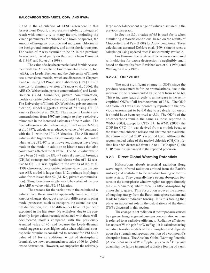
results. In this approach, measurements of correlationsbetween halocarbons are used to evaluate chlorine andbromine relative stratospheric release values. Theserelease rates are used with lifetimes, molecular weights,and the number and type of halogen atoms per moleculeto estimate the effect of a small source gas pulse emissionon stratospheric ozone depletion. In the case of bromineand iodine, the catalytic efficiency for ozone destructionrelative to chlorine is needed and differs from unity partlydue to the different partitioning of the halogen chemicalfamilies. For long-lived chlorocarbons and bromocarbonsthat are well mixed in the troposphere, the semi-empiricalODP definition can be expressed by:
(8-2)
where f is the fractional halogen release factor, α is therelative effectiveness of bromine compared with chlorinefor ozone destruction, τ is the global lifetime, M is themolecular weight, and nCl (nBr) is the number of chlorine(bromine) atoms contained in the compound. CFC-11 sub-scripts indicate quantities for CFC-11, while i subscriptsdenote quantities pertaining to the compound for whichthe ODP is desired. This equation has been altered slightlyfrom the form given in the previous Assessment (Equation1-6, WMO, 2003) because it was less clear how to accountfor compounds with both chlorine and bromine atomsusing the previous form. For very short-lived substances(VSLSs), the location and season of emission affect theamount of halogen that can make it to the stratosphere,making Equation (8-2) an inappropriate choice for ODPestimates of these gases (see Chapter 2 of this Assess-ment, as well as Chapter 2 of WMO, 2003).
8.2.2.1 ATMOSPHERIC LIFETIMES
The lifetimes of atmospheric trace gases given inTables 8-1 and 8-2 have been assessed in Chapter 1. Adetailed explanation of global lifetimes can be found inWMO (2003). For these reported lifetimes, it is assumedthat the gases are uniformly mixed throughout the tropo-sphere. This assumption is less accurate for gases withlifetimes <1/2 year, and is but one reason why single valuesfor global lifetimes, ODPs, or GWPs are less appropriatefor such short-lived gases (see Chapter 2). However, themajority of ozone-depleting substances and their replace-ments have atmospheric lifetimes greater than 2 years,much longer than tropospheric mixing times; hence theirlifetimes, ODPs, and GWPs are not significantly alteredby the location of sources within the troposphere.
8.2.2.2 FRACTIONAL RELEASE FACTORS
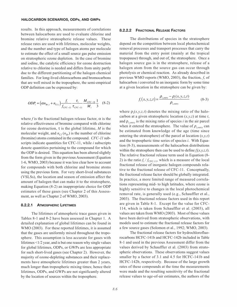
The distributions of species in the stratospheredepend on the competition between local photochemicalremoval processes and transport processes that carry thematerial from the entry point (mainly at the tropicaltropopause) through, and out of, the stratosphere. Once ahalogen source gas is in the stratosphere, release of ahalogen atom from the source gas can occur throughphotolysis or chemical reaction. As already described inprevious WMO reports (WMO, 2003), the fraction, f, ofhalocarbon i converted to an inorganic form by some timeat a given location in the stratosphere can be given by:
(8-3)
where ρi(x,y,z,t) denotes the mixing ratio of the halo-carbon at a given stratospheric location (x,y,z) at time t,and ρi,entry is the mixing ratio of species i in the air parcelwhen it entered the stratosphere. The value of ρi,entry canbe estimated from knowledge of the age (time sinceentering the stratosphere) of the parcel at location (x,y,z)and the tropospheric time series of species i. With Equa-tion (8-3), measurements of the halocarbon distributionswithin the stratosphere then can be used to define fi(x,y,z,t).The relative fractional release term used in Equation (8-2) is the ratio fi / fCFC-11, which is a measure of the localfractional release of inorganic halogen compounds rela-tive to the fractional release of CFC-11. Conceptually,the fractional release factor should be globally integrated.In practice, a more limited range of measured correla-tions representing mid- to high latitudes, where ozone ishighly sensitive to changes in the local photochemicalremoval rate, is generally used (e.g., Schauffler et al.,2003). The fractional release factors used in this reportare given in Table 8-1. Except for the value for CFC-114, which is taken from Schauffler et al. (2003), allvalues are taken from WMO (2003). Most of these valueshave been derived from stratospheric observations, withmodels used to estimate the fractional release factors fora few source gases (Solomon et al., 1992; WMO, 2003).
The fractional release factors for hydrochlorofluo-rocarbons HCFC-141b and HCFC-142b included in Table8-1 and used in the previous Assessment differ from thevalues derived by Schauffler et al. (2003) from strato-spheric observations. These observations suggest valuessmaller by a factor of 3.1 and 4.5 for HCFC-141b andHCFC-142b, respectively. Because of the large growthrates of these compounds at the time the measurementswere made and the resulting sensitivity of the fractionalrelease values to age-of-air estimates, the authors of the
HALOCARBON SCENARIOS, ODPs, AND GWPs
8.6
ODP n nf
f
Mi Br i Cl i
i
CFC
i
CFC
CFC= +( )− −
−α ττ, ,
11 11
111 1
3Mi
f x y z tx y z t
ii entry i
i entry
, , ,( , , , ),
,
( ) =−ρ ρρ
previous Assessment did not adopt these new values. Withno additional estimates available since this disagreementwas discussed in the previous Assessment, the discrep-ancy remains an unresolved issue and we continue to usethe older, model-derived values. Model estimates for allother gases agree with the values estimated from observa-tions to within 2 times the quoted error bars of the obser-vational estimates (Schauffler et al., 2003) except for
HCFC-22. The HCFC-22 value based on observations isabout 17% lower than calculated in Solomon et al. (1992).
8.2.2.3 OZONE DESTRUCTION EFFECTIVENESS
Although the relative effectiveness of brominecompared with chlorine for ozone depletion, referred toas α, is treated as a single, fixed quantity in Equation 8-
HALOCARBON SCENARIOS, ODPs, AND GWPs
8.7
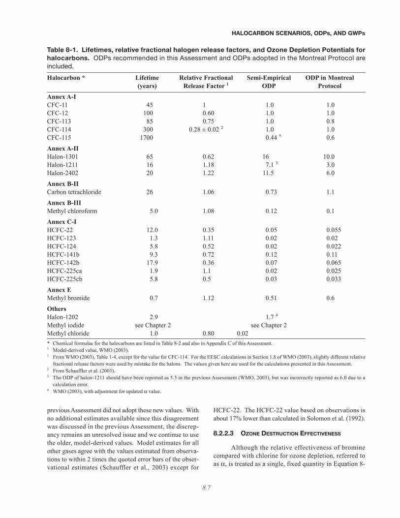
Table 8-1. Lifetimes, relative fractional halogen release factors, and Ozone Depletion Potentials forhalocarbons. ODPs recommended in this Assessment and ODPs adopted in the Montreal Protocol areincluded.
Halocarbon * Lifetime Relative Fractional Semi-Empirical ODP in Montreal(years) Release Factor 1 ODP Protocol
Annex A-ICFC-11 45 1 1.0 1.0CFC-12 100 0.60 1.0 1.0CFC-113 85 0.75 1.0 0.8CFC-114 300 0.28 ± 0.02 2 1.0 1.0CFC-115 1700 0.44 † 0.6
Annex A-IIHalon-1301 65 0.62 16 10.0Halon-1211 16 1.18 7.1 3 3.0Halon-2402 20 1.22 11.5 6.0
Annex B-IICarbon tetrachloride 26 1.06 0.73 1.1
Annex B-IIIMethyl chloroform 5.0 1.08 0.12 0.1
Annex C-IHCFC-22 12.0 0.35 0.05 0.055HCFC-123 1.3 1.11 0.02 0.02HCFC-124 5.8 0.52 0.02 0.022HCFC-141b 9.3 0.72 0.12 0.11HCFC-142b 17.9 0.36 0.07 0.065HCFC-225ca 1.9 1.1 0.02 0.025HCFC-225cb 5.8 0.5 0.03 0.033
Annex EMethyl bromide 0.7 1.12 0.51 0.6
OthersHalon-1202 2.9 1.7 4
Methyl iodide see Chapter 2 see Chapter 2Methyl chloride 1.0 0.80 0.02* Chemical formulae for the halocarbons are listed in Table 8-2 and also in Appendix C of this Assessment.† Model-derived value, WMO (2003).1 From WMO (2003), Table 1-4, except for the value for CFC-114. For the EESC calculations in Section 1.8 of WMO (2003), slightly different relative
fractional release factors were used by mistake for the halons. The values given here are used for the calculations presented in this Assessment.2 From Schauffler et al. (2003).3 The ODP of halon-1211 should have been reported as 5.3 in the previous Assessment (WMO, 2003), but was incorrectly reported as 6.0 due to a
calculation error.4 WMO (2003), with adjustment for updated α value.
2 and in the calculation of EESC elsewhere in thisAssessment Report, it represents a globally integratedresult with sensitivity to many factors, including thekinetic parameters for chlorine and bromine species, theamount of inorganic bromine and inorganic chlorine inthe background atmosphere, and atmospheric transport.The value of α was assumed to be 45 in the previousAssessment, based partly on the results from Daniel etal. (1999) and Ko et al. (1998).
The value of α has been recalculated for this Assess-ment with the Atmospheric Environmental Research, Inc.(AER), the Leeds-Bremen, and the University of Illinoistwo-dimensional models, which are discussed in Chapters2 and 6. Using Jet Propulsion Laboratory (JPL) JPL-05kinetics (preliminary version of Sander et al., 2006), theAER (D. Weisenstein, private communication) and Leeds-Bremen (B.-M. Sinnhuber, private communication)models calculate global values of 61 and 71, respectively.The University of Illinois (D. Wuebbles, private commu-nication) model suggests a value of 57 using JPL-02kinetics (Sander et al., 2002). The change in kinetics rec-ommendations from 1997 are thought to play a relativelyminor role in the increased estimates of the α value. TheLeeds-Bremen model, when using JPL-97 rates (DeMoreet al., 1997), calculates a reduced α value of 64 comparedwith the 71 with the JPL-05 kinetics. The AER modelvalue is also higher than its previously calculated valuewhen using JPL-97 rates; however, changes have beenmade in the model in addition to kinetic rates that alsocould have affected the α value. The AER value wouldhave been 52 with the JPL-97 rates if a methyl bromide(CH3Br) stratosphere fractional release value of 1.12 rela-tive to CFC-11 was applied to the results of Ko et al.(1998); however, the calculated release value from the cur-rent AER model is larger than 1.12, perhaps implying avalue for α lower than 52 (M. Ko, private communica-tion). Thus, there is no simple way to be certain of the pre-cise AER α value with JPL-97 kinetics.
The reasons for the variations in the calculated αvalues from these models apparently arise not fromkinetics changes alone, but also from differences in othermodel processes, such as transport, the ozone loss spa-tial distribution, etc. The differences have not yet beenexplained in the literature. Nevertheless, due to the con-sistently larger values recently calculated with these well-documented models compared with the previouslyassumed value of 45, and because the Leeds-Bremenmodel suggests an even higher value when additional strat-ospheric bromine is considered to account for VSLSs (avalue of 73 for an additional 6 ppt of stratosphericbromine), we now recommend an α value of 60 for globalozone destruction. However, we emphasize the relatively
large model-dependent range of values discussed in theprevious paragraph.
In Section 8.3, a value of 65 is used for α whensimulating Antarctic conditions, based on the results ofChipperfield and Pyle (1998) for Arctic conditions. Thesecalculations assumed DeMore et al. (1994) kinetic rates; acalculation using updated rates is not currently available.
For fluorine, the relative effectiveness comparedwith chlorine for ozone destruction is negligibly smallbased on the results from Ravishankara et al. (1994) andWallington et al. (1995).
8.2.2.4 ODP VALUES
The most significant change in ODPs since theprevious Assessment is for the bromocarbons, due to theincrease in the recommended value of α from 45 to 60.This α increase leads directly to an increase in the semi-empirical ODPs of all bromocarbons of 33%. The ODPof halon-1211 was also incorrectly reported in the pre-vious Assessment to be 6.0 due to a calculation error;it should have been reported as 5.3. The ODPs of thechlorocarbons remain the same as those reported inWMO (2003), except for CFC-114. In WMO (2003), theODP for CFC-114 was derived from a model; becausethe fractional chlorine release and lifetime are available,the semi-empirical ODP is reported here. Although therecommended value of the methyl chloride (CH3Cl) life-time has been decreased from 1.3 to 1.0 (Chapter 1), theODP remains unchanged to the reported precision.
8.2.3 Direct Global Warming Potentials
Halocarbons absorb terrestrial radiation (longwavelength infrared radiation emitted from the Earth’ssurface) and contribute to the radiative forcing of the cli-mate system. They generally have strong absorption fea-tures in the atmospheric window region (at approximately8-12 micrometers) where there is little absorption byatmospheric gases. This absorption reduces the amountof outgoing energy from the Earth-atmosphere system andleads to a direct radiative forcing. It is this forcing thatplays an important role in the calculations of the directGWPs discussed in this section.
The change in net radiation at the tropopause causedby a given change in greenhouse gas concentration or massis referred to as radiative efficiency. Radiative efficiencyhas units of W m-2 ppb-1 or W m-2 kg-1; it is calculated usingradiative transfer models of the atmosphere and dependsupon the strength and spectral position of a compound’sabsorption bands. The Absolute Global Warming Potential(AGWP) has units of W m-2 ppb-1 yr or W m-2 k-1 yr andquantifies the future integrated radiative forcing of a unit
HALOCARBON SCENARIOS, ODPs, AND GWPs
8.8
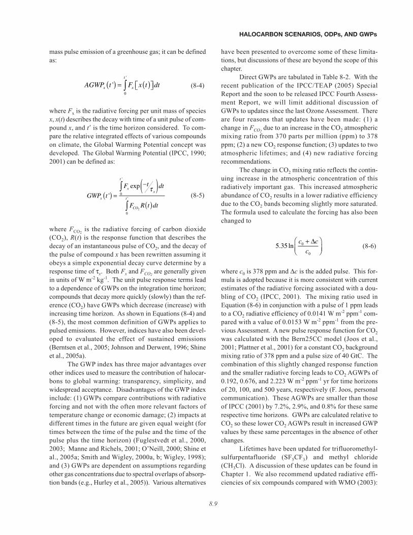
mass pulse emission of a greenhouse gas; it can be definedas:
(8-4)
where Fx is the radiative forcing per unit mass of speciesx, x(t) describes the decay with time of a unit pulse of com-pound x, and t9 is the time horizon considered. To com-pare the relative integrated effects of various compoundson climate, the Global Warming Potential concept wasdeveloped. The Global Warming Potential (IPCC, 1990;2001) can be defined as:
(8-5)
where FCO2is the radiative forcing of carbon dioxide
(CO2), R(t) is the response function that describes thedecay of an instantaneous pulse of CO2, and the decay ofthe pulse of compound x has been rewritten assuming itobeys a simple exponential decay curve determine by aresponse time of τx. Both Fx and FCO2
are generally givenin units of W m-2 kg-1. The unit pulse response terms leadto a dependence of GWPs on the integration time horizon;compounds that decay more quickly (slowly) than the ref-erence (CO2) have GWPs which decrease (increase) withincreasing time horizon. As shown in Equations (8-4) and(8-5), the most common definition of GWPs applies topulsed emissions. However, indices have also been devel-oped to evaluated the effect of sustained emissions(Berntsen et al., 2005; Johnson and Derwent, 1996; Shineet al., 2005a).
The GWP index has three major advantages overother indices used to measure the contribution of halocar-bons to global warming: transparency, simplicity, andwidespread acceptance. Disadvantages of the GWP indexinclude: (1) GWPs compare contributions with radiativeforcing and not with the often more relevant factors oftemperature change or economic damage; (2) impacts atdifferent times in the future are given equal weight (fortimes between the time of the pulse and the time of thepulse plus the time horizon) (Fuglestvedt et al., 2000,2003; Manne and Richels, 2001; O’Neill, 2000; Shine etal., 2005a; Smith and Wigley, 2000a, b; Wigley, 1998);and (3) GWPs are dependent on assumptions regardingother gas concentrations due to spectral overlaps of absorp-tion bands (e.g., Hurley et al., 2005)). Various alternatives
have been presented to overcome some of these limita-tions, but discussions of these are beyond the scope of thischapter.
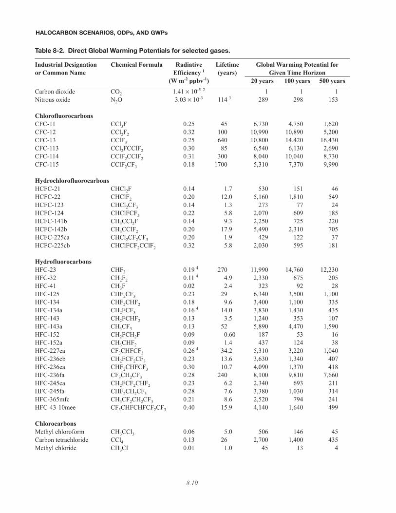
Direct GWPs are tabulated in Table 8-2. With therecent publication of the IPCC/TEAP (2005) SpecialReport and the soon to be released IPCC Fourth Assess-ment Report, we will limit additional discussion ofGWPs to updates since the last Ozone Assessment. Thereare four reasons that updates have been made: (1) achange in FCO2
due to an increase in the CO2 atmosphericmixing ratio from 370 parts per million (ppm) to 378ppm; (2) a new CO2 response function; (3) updates to twoatmospheric lifetimes; and (4) new radiative forcingrecommendations.
The change in CO2 mixing ratio reflects the contin-uing increase in the atmospheric concentration of thisradiatively important gas. This increased atmosphericabundance of CO2 results in a lower radiative efficiencydue to the CO2 bands becoming slightly more saturated.The formula used to calculate the forcing has also beenchanged to
(8-6)
where c0 is 378 ppm and ∆c is the added pulse. This for-mula is adopted because it is more consistent with currentestimates of the radiative forcing associated with a dou-bling of CO2 (IPCC, 2001). The mixing ratio used inEquation (8-6) in conjunction with a pulse of 1 ppm leadsto a CO2 radiative efficiency of 0.0141 W m-2 ppm-1 com-pared with a value of 0.0153 W m-2 ppm-1 from the pre-vious Assessment. A new pulse response function for CO2was calculated with the Bern25CC model (Joos et al.,2001; Plattner et al., 2001) for a constant CO2 backgroundmixing ratio of 378 ppm and a pulse size of 40 GtC. Thecombination of this slightly changed response functionand the smaller radiative forcing leads to CO2 AGWPs of0.192, 0.676, and 2.223 W m-2 ppm-1 yr for time horizonsof 20, 100, and 500 years, respectively (F. Joos, personalcommunication). These AGWPs are smaller than thoseof IPCC (2001) by 7.2%, 2.9%, and 0.8% for these samerespective time horizons. GWPs are calculated relative toCO2 so these lower CO2 AGWPs result in increased GWPvalues by these same percentages in the absence of otherchanges.
Lifetimes have been updated for trifluoromethyl-sulfurpentafluoride (SF5CF3) and methyl chloride(CH3Cl). A discussion of these updates can be found inChapter 1. We also recommend updated radiative effi-ciencies of six compounds compared with WMO (2003):
HALOCARBON SCENARIOS, ODPs, AND GWPs
8.9
AGWP t F x t dtx x
t
''
( ) = ( ) ∫0
GWP t
F t dt
F R t dtx
xx
t
CO
t'
exp'
'( ) =
−( )( )
∫
∫
τ0
02
5 35 0
0
. lnc c
c
+ ∆
HALOCARBON SCENARIOS, ODPs, AND GWPs
8.10
Table 8-2. Direct Global Warming Potentials for selected gases.
Industrial Designation Chemical Formula Radiative Lifetime Global Warming Potential foror Common Name Efficiency 1 (years) Given Time Horizon
(W m-2 ppbv-1) 20 years 100 years 500 yearsCarbon dioxide CO2 1.41 × 10⁻⁵ 2 1 1 1Nitrous oxide N2O 3.03 × 10⁻³ 114 3 289 298 153
ChlorofluorocarbonsCFC-11 CCl3F 0.25 45 6,730 4,750 1,620CFC-12 CCl2F2 0.32 100 10,990 10,890 5,200CFC-13 CClF3 0.25 640 10,800 14,420 16,430CFC-113 CCl2FCClF2 0.30 85 6,540 6,130 2,690CFC-114 CClF2CClF2 0.31 300 8,040 10,040 8,730CFC-115 CClF2CF3 0.18 1700 5,310 7,370 9,990
HydrochlorofluorocarbonsHCFC-21 CHCl2F 0.14 1.7 530 151 46HCFC-22 CHClF2 0.20 12.0 5,160 1,810 549HCFC-123 CHCl2CF3 0.14 1.3 273 77 24HCFC-124 CHClFCF3 0.22 5.8 2,070 609 185HCFC-141b CH3CCl2F 0.14 9.3 2,250 725 220HCFC-142b CH3CClF2 0.20 17.9 5,490 2,310 705HCFC-225ca CHCl2CF2CF3 0.20 1.9 429 122 37HCFC-225cb CHClFCF2CClF2 0.32 5.8 2,030 595 181
HydrofluorocarbonsHFC-23 CHF3 0.19 4 270 11,990 14,760 12,230HFC-32 CH2F2 0.11 4 4.9 2,330 675 205HFC-41 CH3F 0.02 2.4 323 92 28HFC-125 CHF2CF3 0.23 29 6,340 3,500 1,100HFC-134 CHF2CHF2 0.18 9.6 3,400 1,100 335HFC-134a CH2FCF3 0.16 4 14.0 3,830 1,430 435HFC-143 CH2FCHF2 0.13 3.5 1,240 353 107HFC-143a CH3CF3 0.13 52 5,890 4,470 1,590HFC-152 CH2FCH2F 0.09 0.60 187 53 16HFC-152a CH3CHF2 0.09 1.4 437 124 38HFC-227ea CF3CHFCF3 0.26 4 34.2 5,310 3,220 1,040HFC-236cb CH2FCF2CF3 0.23 13.6 3,630 1,340 407HFC-236ea CHF2CHFCF3 0.30 10.7 4,090 1,370 418HFC-236fa CF3CH2CF3 0.28 240 8,100 9,810 7,660HFC-245ca CH2FCF2CHF2 0.23 6.2 2,340 693 211HFC-245fa CHF2CH2CF3 0.28 7.6 3,380 1,030 314HFC-365mfc CH3CF2CH2CF3 0.21 8.6 2,520 794 241HFC-43-10mee CF3CHFCHFCF2CF3 0.40 15.9 4,140 1,640 499
ChlorocarbonsMethyl chloroform CH3CCl3 0.06 5.0 506 146 45Carbon tetrachloride CCl4 0.13 26 2,700 1,400 435Methyl chloride CH3Cl 0.01 1.0 45 13 4
HALOCARBON SCENARIOS, ODPs, AND GWPs
8.11
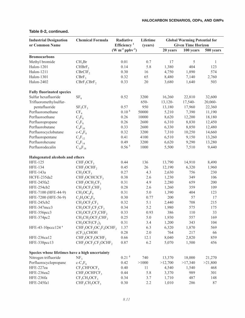
Table 8-2, continued.
Industrial Designation Chemical Formula Radiative Lifetime Global Warming Potential foror Common Name Efficiency 1 (years) Given Time Horizon
(W m-2 ppbv-1) 20 years 100 years 500 yearsBromocarbonsMethyl bromide CH3Br 0.01 0.7 17 5 1Halon-1201 CHBrF2 0.14 5.8 1,380 404 123Halon-1211 CBrClF2 0.30 16 4,750 1,890 574Halon-1301 CBrF3 0.32 65 8,480 7,140 2,760Halon-2402 CBrF2CBrF2 0.33 20 3,680 1,640 503
Fully fluorinated speciesSulfur hexafluoride SF6 0.52 3200 16,260 22,810 32,600Trifluoromethylsulfur- 650- 13,120- 17,540- 20,060-
pentafluoride SF5CF3 0.57 950 13,180 17,960 22,360Perfluoromethane CF4 0.10 4 50000 5,210 7,390 11,190Perfluoroethane C2F6 0.26 10000 8,620 12,200 18,180Perfluoropropane C3F8 0.26 2600 6,310 8,830 12,450Perfluorobutane C4F10 0.33 2600 6,330 8,850 12,480Perfluorocyclobutane c-C4F8 0.32 3200 7,310 10,250 14,660Perfluoropentane C5F12 0.41 4100 6,510 9,150 13,260Perfluorohexane C6F14 0.49 3200 6,620 9,290 13,280Perfluorodecalin C10F18 0.56 5 1000 5,500 7,510 9,440
Halogenated alcohols and ethersHFE-125 CHF2OCF3 0.44 136 13,790 14,910 8,490HFE-134 CHF2OCHF2 0.45 26 12,190 6,320 1,960HFE-143a CH3OCF3 0.27 4.3 2,630 756 230HCFE-235da2 CHF2OCHClCF3 0.38 2.6 1,230 349 106HFE-245fa2 CHF2OCH2CF3 0.31 4.9 2,280 659 200HFE-254cb2 CH3OCF2CHF2 0.28 2.6 1,260 359 109HFE-7100 (HFE-44-9) CH3OC4F9 0.31 5.0 1,390 404 123HFE-7200 (HFE-56-9) C2H5OC4F9 0.30 0.77 200 57 17HFE-245cb2 CH3OCF2CF3 0.32 5.1 2,440 708 215HFE-347mcc3 CH3OCF2CF2CF3 0.34 5.2 1,980 575 175HFE-356pcc3 CH3OCF2CF2CHF2 0.33 0.93 386 110 33HFE-374pc2 CH3CH2OCF2CHF2 0.25 5.0 1,930 557 169
CH3OCF(CF3)2 0.31 3.4 1,200 343 104HFE-43-10pccc124 a CHF2OCF2OC2F4OCHF2 1.37 6.3 6,320 1,870 569
(CF3)2CHOH 0.28 2.0 764 217 66HFE-236ca12 CHF2OCF2OCHF2 0.66 12.1 8,040 2,820 859HFE-338pcc13 CHF2OCF2CF2OCHF2 0.87 6.2 5,070 1,500 456
Species whose lifetimes have a high uncertaintyNitrogen trifluoride NF3 0.21 4 740 13,370 18,000 21,270Perfluorocyclopropane c-C3F6 0.42 >1000 >12,700 >17,340 >21,800HFE-227ea CF3CHFOCF3 0.40 11 4,540 1,540 468HFE-236ea2 CHF2OCHFCF3 0.44 5.8 3,370 989 301HFE-236fa CF3CH2OCF3 0.34 3.7 1,710 487 148HFE-245fa1 CHF2CH2OCF3 0.30 2.2 1,010 286 87
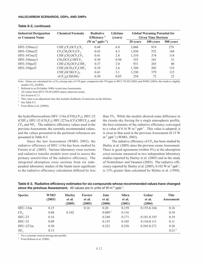
the hydrofluorocarbons HFC-134a (CFH2CF3), HFC-23(CHF3), HFC-32 (CH2F2), HFC-227ea (CF3CHFCF3), andCF4 and NF3. The radiative efficiency values used in theprevious Assessment, the currently recommended values,and the values presented in the pertinent references arepresented in Table 8-3.
Since the last Assessment (WMO, 2003), theradiative efficiency of HFC-134a has been studied byForster et al. (2005). Various laboratory cross sectionsand radiative transfer models were used to assess theprimary sensitivities of the radiative efficiency. Theintegrated absorption cross sections from six inde-pendent laboratory studies of the bands most significantto the radiative efficiency calculation differed by less
than 5%. While the models showed some difference inthe cloudy-sky forcing for a single atmospheric profile,the best estimates of the radiative efficiency convergedto a value of 0.16 W m-2 ppb-1. This value is adopted; itis close to that used in the previous Assessment (0.15 Wm-2 ppb-1) (WMO, 2003).
The radiative efficiency of CF4 has been studied byHurley et al. (2005) since the previous ozone Assessment.There is good agreement (within 4%) in the absorptioncross sections measured in two independent laboratorystudies reported by Hurley et al. (2005) and in the studyof Nemtchinov and Varanasi (2003). The radiative effi-ciency reported by Hurley et al. (2005), 0.102 W m-2 ppb-1,is 15% greater than calculated by Myhre et al. (1998).
HALOCARBON SCENARIOS, ODPs, AND GWPs
8.12
Table 8-2, continued.
Industrial Designation Chemical Formula Radiative Lifetime Global Warming Potential foror Common Name Efficiency 1 (years) Given Time Horizon
(W m-2 ppbv-1) 20 years 100 years 500 yearsHFE-329mcc2 CHF2CF2OCF2CF3 0.49 6.8 3,060 919 279HFE-338mcf2 CF3CH2OCF2CF3 0.43 4.3 1,920 552 168HFE-347mcf2 CHF2CH2OCF2CF3 0.41 2.8 1,310 374 114HFE-356mec3 CH3OCF2CHFCF3 0.30 0.94 355 101 31HFE-356pcf2 CHF2CH2OCF2CHF2 0.37 2.0 931 265 80HFE-356pcf3 CHF2OCH2CF2CHF2 0.39 3.6 1,760 502 153
CHF2OCH(CF3)2 0.41 3.1 1,330 379 115-(CF2)4CH(OH)- 0.30 0.85 254 72 22
Note: Values are calculated for a CO2 mixing ratio of 378 ppm, compared with 370 ppm in IPCC/TEAP (2005) and WMO (2003); this leads to slightlysmaller CO2 AGWPs.
a Referred to as H-Galden 1040x in previous Assessments.1 All values from IPCC/TEAP (2005) unless otherwise noted.2 See Section 8.2.3.3 This value is an adjustment time that includes feedbacks of emissions on the lifetime.4 See Table 8-3.5 From Shine et al. (2005b).
Table 8-3. Radiative efficiency estimates for six compounds whose recommended values have changedsince the previous Assessment. All values are in units of W m-2 ppb-1.
Species WMO Hurley Forster Jain Sihra Gohar This (2003) et al. et al. et al. et al. et al. Assessment
(2005) (2005) (2000) (2001) (2004)HFC-134a 0.15 0.16 0.20 0.159 0.155-0.166 0.16CF4 0.08 0.102 0.089 1 0.116 0.10HFC-23 0.16 0.248 0.171 0.181-0.193 0.19HFC-32 0.09 0.155 0.105 0.110-0.111 0.11HFC-227ea 0.30 0.322 0.256 0.243-0.271 0.26NF3 0.13 0.21 2
1 For a constant vertical mixing ratio profile.2 From Robson et al. (2006).
About a 10% increase is explained by the larger cross sec-tion and the remaining 5% is believed to be due to dif-fering radiative transfer codes employed.
Since the last ozone Assessment, radiative effi-ciencies of HFC-23, HFC-32, and HFC-227ea have beenstudied by Gohar et al. (2004), using two independentsets of radiation codes. There is a greater than 20% dif-ference in the calculated radiative efficiencies of thesegases reported by Sihra et al. (2001) and Jain et al.(2000), both of which were considered in the previousAssessment. At the time of the previous Assessment,the reason for the differences was not clear and averagesof the two datasets were used. While the reason for thedifferences between the Jain et al. and Sihra et al. valuesare still unknown, the results of Gohar et al. (2004) sup-port the values given by Sihra et al. (2001), leading toan update of the recommendations given in Table 8-3.The calculations by Gohar et al. (2004) also illustratethe sensitivity of the radiative efficiency calculations tothe particular model choice.
The radiative efficiency of NF3 has been re-eval-uated recently by Robson et al. (2006). The radiativeefficiency used in previous Assessments (IPCC, 2001;WMO, 1999, 2003) was calculated from the absorptioncross section data of Molina et al. (1995) by K.P. Shineusing the simple radiative method given in Pinnock etal. (1995), as no radiative efficiency was provided in theMolina et al. (1995) work. The Robson et al. (2006)study suggests that the more intense infrared (IR) fea-tures reported by Molina et al. (1995) were saturated,causing the inferred radiative efficiency to be too small.Molina et al. (1995) did not report the precise conditionsused to derive their absorption cross section values,making an unambiguous evaluation of the importanceof saturation impossible. We adopt the radiative effi-ciency of 0.21 W m-2 ppb-1 from the more comprehen-sive study by Robson et al. (2006).
The 2σ uncertainty associated with the directGWPs shown is estimated to be ±35%. This value hasbeen adopted from previous ozone and climate Assess-ments (IPCC, 2001; WMO, 2003; IPCC/TEAP, 2005) andis primarily due to uncertainties in the radiative efficien-cies and lifetimes of the halocarbons and to uncertaintiesin our understanding of the carbon cycle (IPCC, 2001).However, because the uncertainties in the carbon cycle arethought to be an important part of this uncertainty, the errorin the relative GWP values among halocarbons should beless than 35% (IPCC, 2001).
The indirect radiative forcing and indirect GWPsof a species quantify the radiative effects from changes inabundances of other greenhouse gases resulting from the
addition of the species considered. Because the indirectforcing and GWPs due to stratospheric ozone loss dependon the future evolution of stratospheric ozone and thus onthe specific ODS emission scenario, these are presented inSection 8.5 of this chapter, after the halocarbon scenariosare discussed.
8.2.4 Degradation Products and TheirImplications for ODPs and GWPs
Degradation products of CFCs, HCFCs, and HFCshave been discussed in IPCC/TEAP (2005). The mainconclusion was that the intermediate degradation productsof most long-lived CFCs, HCFCs, and HFCs have shorterlifetimes than the source gases, and therefore have loweratmospheric concentrations and smaller radiative forcings.Intermediate products and final products are removed fromthe atmosphere via deposition and washout processes andmay accumulate in oceans, lakes, and other aquatic reser-voirs. Trifluoroacetic acid is a persistent degradationproduct of some HCFCs and HFCs and is removed fromthe atmosphere mainly by wet deposition. Its sources (nat-ural and anthropogenic), sinks, and potential environ-mental effects have been reviewed by Tang et al. (1998),Solomon et al. (2003), and IPCC/TEAP (2005). The avail-able environmental risk assessment and monitoring dataindicate that the source of trifluoroacetic acid from thedegradation of HCFCs and HFCs will not result in envi-ronmental concentrations capable of significant eco-system damage.
8.3 FUTURE HALOCARBON SOURCE GASCONCENTRATIONS
8.3.1 Introduction
Projections of future atmospheric halocarbonmixing ratios require knowledge of future emissions andatmospheric/oceanic loss rates in addition to currentatmospheric abundances. In this section, we use estimatesof these quantities in a simple box model to calculateaverage future surface mixing ratios, which are assumedto be related to mean atmospheric mixing ratios by a fixedfactor. These calculated mixing ratios are used to generateequivalent effective stratospheric chlorine (EESC) esti-mates, which are used to evaluate the effects of differenthalocarbon production/emission scenarios and hypothet-ical test cases. The lifetimes presented in Table 8-1 (seealso Chapter 1) are estimated from the loss rates of theODSs and are used in the box model. Any future changesin the hydroxyl radical (OH) amount (IPCC, 2001) and/or
HALOCARBON SCENARIOS, ODPs, AND GWPs
8.13
distribution, and any changes in circulation (see, e.g.,Chapters 5 and 6) that might affect lifetimes, are neglected.To include more complicated atmospheric interactionssuch as these, more sophisticated two-dimensional (2-D)and three-dimensional (3-D) atmospheric models shouldbe used.
The box model approach used here has also beenused in previous Assessments (WMO, 1995; 1999; 2003).Global mean mixing ratios are calculated using theequation
(8-7)
where ρ is the global mean mixing ratio (in ppt), τ is thetotal atmospheric lifetime, E is the emission rate (inkg/year), and F is the factor that relates the mass emittedto the global mean mixing ratio, given by
(8-8)
where F is in units of ppt/kg, and M is the molecularweight (in kg/mole). The i subscripts refer to the speciesconsidered in the calculation. As in the previous ozoneAssessment, the calculated global mean mixing ratios aremultiplied by a factor of 1.07 to represent surface mixingratios. This factor is meant to account for the generaldecrease of the halocarbon mixing ratios with altitudeabove the tropopause. Using a constant factor such asthis neglects the dependence of this factor on the partic-ular species and neglects any change in this factor thatcould be caused by changes in circulation or by the vari-ability of the surface emission (and the resulting vari-ability in the atmospheric vertical distribution).
Accurate projections of emissions require an under-standing of the amount of halocarbons in equipment andproduct banks, the rates of release from these banks, thequantity of equipment and products using ODSs that willbe put into service, emissive uses, and the future productionof ODSs. Banks here are defined as the quantity of ODSsproduced but not yet emitted to the atmosphere. Due to theimportance of policy decisions, energy cost, technologicaladvancement, and economic growth rates in estimatingfuture production and banks, the uncertainty level in futureemissions remains high. However, with each passing year,as more years of emissions can be calculated from atmos-pheric abundance observations and fewer years remain forthe legal consumption of ODSs under the Montreal Proto-col, future projections should become more constrained.
Scenarios and test cases have been developed todescribe the possible range of future atmospheric abun-dances of ODSs. These cases are generated using the cur-rent understanding of global production, emission, andbanks of the most widely used halocarbons. Scenario A1is meant to represent the current baseline or “best guess”scenario, analogous to the Ab scenario from the previousAssessment. An estimated “maximum” scenario, devel-oped for previous Assessments, is not generated for thisAssessment because developed and developing countrieshave produced less CFCs in 2000-2004 than allowed underthe Montreal Protocol and the HCFC production in devel-oping countries is not controlled before 2016. Hence, anyattempt to develop such a scenario would be largely spec-ulative on our part. Indeed, it is this uncertainty in futureHCFC emission that represents a major reason for thedifference that will be discussed later between the cur-rent A1 scenario and the comparable Ab scenario of theprevious Assessment.
Consistent with past Assessments, our approach torelating annual production, emission, and banks sizesplaces most confidence on the emission values calculatedfrom atmospheric observations and global lifetimes. Accu-rate estimates of yearly averaged ODS emissions fromatmospheric observations are possible when global life-times are long and accurately known, and accurate globalmixing ratio observations of ODSs are available. Thisapproach, when used to estimate current bank sizes fromhistoric production and emission data, is sometimesreferred to as a top-down approach. In past Assessments,any inconsistency between mixing ratio observations andemission estimates based on the best knowledge of ODSproduction, sales, and application-specific release func-tions was eliminated by adjusting the bank size so theemissions would be consistent with the observations. Thebank that remained after the sum of adjustments for allyears was used in the future projections. Because the bankis an accumulating difference often between two largenumbers, this method has an uncertainty that is difficult toquantify and can lead to unreasonable bank sizes; indeedthe estimate of no bank in 2002 for CFC-12 in the previousozone Assessment is such an example (IPCC/TEAP, 2005).One way an unreasonable bank could be attained is in acase in which annual production numbers are accuratelyknown, but the atmospheric lifetime assumed is incorrect.In such a case, a lifetime that is too small (large) will resultin an annual release from the bank that must be too large(small) for calculated mixing ratios to agree with observa-tions. Such a situation would occur year after year andcould result in a potentially significant error in the bankestimate today, depending on the compound (Daniel et al.,
HALOCARBON SCENARIOS, ODPs, AND GWPs
8.14
d
dtFEi
i ii
i
ρ ρτ
= −
FMi
i
=× −5 68 10 9.
2006). But without an independent estimate of bank size,such an error would be difficult to identify.
A different approach for determining bank sizes istaken in this Assessment because of the new independentestimates of bank sizes for several ODSs for the years 2002and 2015 (Clodic and Palandre, 2004; IPCC/TEAP, 2005).These estimates are independent of atmospheric abun-dance observations and have been determined from thenumber of units of equipment that use a particular ODSand the amount of ODS in each unit. This is commonlyreferred to as a bottom-up approach. An extensive expla-nation of this methodology can be found in IPCC/TEAP(2005). Future emissions until 2015 estimated in thisAssessment are calculated by beginning with the 2002bottom-up bank from IPCC/TEAP (2005), and then byadding annual production and applying a constant annualbank emission factor needed to attain the bottom-up bankestimated in 2015 by IPCC/TEAP (2005). After 2015,emissions are calculated using the same constant bankemission factors as immediately before 2015. Thus, whenbottom-up bank size estimates for 2002 and 2015 are avail-able for a particular ODS, the scenarios in this chapter areconsistent with them in most cases.
Bottom-up estimates are also not without prob-lems; indeed bottom-up 2002 emission estimates for CFC-11, HCFC-141b, and HCFC-142b (IPCC/TEAP, 2005),which are dominated by emissions from foams, are smallerby more than a factor of two when compared with what isneeded to be consistent with mixing ratio observations.Nevertheless, it is felt that these bottom-up bank estimatesrepresent an important new constraint to current bank sizesthat warrants a large role in the future projections in thischapter. In Sections 8.3.2.1 and 8.3.4, more discussion ofthe uncertainties involved with bottom-up and top-downemission estimates and their potential effects on the sce-narios is presented.
8.3.2 Baseline Scenario (A1)
In this chapter, estimates of future banks and emis-sions have been calculated for most ODSs using annualproduction reported to the United Nations EnvironmentProgramme (UNEP, 2005), emissions estimated fromatmospheric observations, and bank size estimates basedon the bottom-up calculations of IPCC/TEAP (2005). Thespecific information used for each ODS considered isdescribed in Table 8-4. Due to the uncertainty in theimportance of and likely future trends in very short-lived(τ < ~0.5 years) organic bromine and chlorine sourcegases, they are not considered in any of these scenarios.However, the bromocarbons considered in this chaptercannot explain the entire stratospheric inorganic bromine
abundance alone, so the very short-lived gases may proveto be important. Detailed information about these com-pounds can be found in Chapter 2.
It should be noted that the assumptions made in cal-culating the baseline scenario are critical to the interpreta-tion of the reduced production and emission scenariosbased on it. For example, if the production and/or banksizes and/or future production rates are underestimated inthe baseline scenario, the “no emission/production” resultspresented in the scenarios would be underestimates of thepotential reduction benefit.
8.3.2.1 EMISSIONS
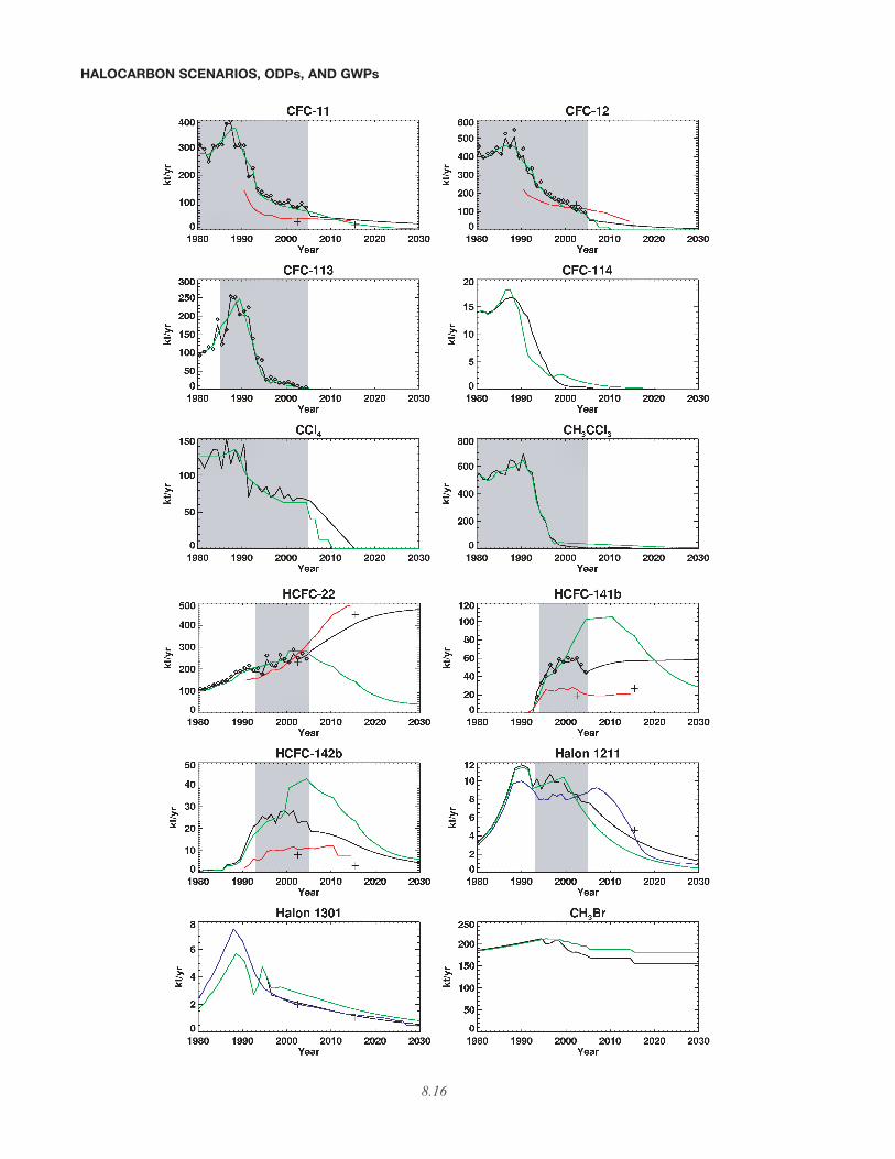
In Figure 8-1, the emission estimates from the 1-box model for the baseline scenario, A1, are comparedwith those of the Ab “best guess” scenario from the pre-vious Assessment, with the IPCC/TEAP (2005) (business-as-usual (BAU) scenario) emissions, with the emissionsof Clodic and Palandre (2004), and with the emissions cal-culated using the 12-box model discussed in Chapter 1.The emissions calculated with the 1-box model are calcu-lated directly from mixing ratio observations (those shadedin Table 8-5) as are the emissions calculated with the 12-box model. The 12-box model, by having some verticalresolution, includes some changes in atmospheric lifetimesdue to variations in atmospheric abundance distributionscaused by increasing or decreasing trends; hence, the 12-box model can presumably better determine the relation-ship between surface mixing ratios and global averagesand can better estimate changes in global lifetimes thatarise from different atmospheric distributions. The com-parisons between the A1 estimated emissions (1-boxmodel) and the 12-box emissions are good most times, butdo show some systematic differences. Throughout themeasurement periods (shaded regions in the figure), the12-box model consistently estimates more emission thanthe 1-box model, with the cumulative differences rangingfrom a 1.2% higher emission for HCFC-141b through themeasurement period as calculated by the 12-box model, toa 6.3% higher emission for CFC-12. There are also notice-able differences between A1 and Ab emissions, many ofwhich are due to the additional information acquired fromcontinued measurements over the past 4 years. Importantdifferences between A1 and Ab include the larger futureemissions of CFC-11 and CFC-12, due to their larger esti-mated banks in A1. The CFC-11 increase in emissionpast 2010 is also due to a decrease of the bank releaserate from plastic foams. The CFC-11 and CFC-12 banksize differences as calculated by the bottom-up method(IPCC/TEAP, 2005) and the top-down method of WMO(2003) have been shown by Daniel et al. (2006) to be large
HALOCARBON SCENARIOS, ODPs, AND GWPs
8.15
HALOCARBON SCENARIOS, ODPs, AND GWPs
8.16
8.17
HALOCARBON SCENARIOS, ODPs, AND GWPs
Table 8-4. Assumptions made in obtaining production and emission estimates for the baseline A1 sce-nario.
General Approach for All Species
Production: For the years when production is reported to UNEP, reported values (or best estimates of production valuesfor cases in which reporting is incomplete or reporting is made by classes of compounds) are used. Beforethis, WMO (2003) production values are generally used. In the future, annual figures are determined fromthe lesser of the Montreal Protocol limitations and the most recent annual estimates.
Emission: For the years when abundance observations are available, emissions are calculated using the box modeldescribed in Section 8.3.1 with the lifetimes of Table 8-1. Emissions before this are usually consistent withWMO (2003) but are also forced to yield mixing ratios that meld smoothly into the measurement record.Future emissions are determined in order to yield banks consistent with IPCC/TEAP (2005).
Bank: The bank assumed to be in place at the start of the measurement record is set at such a value that the IPCC/TEAP(2005) bank for 2002 is attained; the future annual fractional bank release is adjusted so that the IPCC/TEAP(2005) bank for 2015 is attained.
Approach for Specific Species
Species Description
CFC-11 Production:1950-1985: WMO (2003)1986, 1989-2004: UNEP * 1987-1988: McCulloch et al. (2001)2005-2006: Fixed at 2004 levels for Article 5(1) countries, with no other production2007-2009: Protocol limits on Article 5(1) countries, with no other production2010-on: No production
Emission:1980-2004: Emissions calculated from observations2005-on: Emission is a constant fraction of the bank, determined to give a bank in 2015 consistent with
IPCC/TEAP (2005)
CFC-12 Production:Same as CFC-11 except:1987-1988: Interpolated from 1986 and 1989 values2005-2006: Protocol limits for Article 5(1) countries with no other production
Emission:Same formalism as for CFC-11
Figure 8-1. Comparison of scenario A1 emissions (black) with those of scenario Ab of the previousAssessment (green), the emissions of Clodic and Palandre (2004) (red), the IPCC/TEAP (2005) emissions(crosses), and emissions calculated from atmospheric abundance observations using a 12-box model (smalldiamonds), all in units of kilotons per year. Corrected data are used for emissions of halon-1211 according toTEAP (2005) and hence differ from the data reported in IPCC/TEAP (2005). Also shown for halon-1301 arethe emissions estimates from the 2002 report of the Halons Technical Options Committee (HTOC) (UNEP,2003) and, for halon-1211, updates to that report (blue curves). Shaded regions indicate years for which A1emissions are determined with a 1-box model (see text) so that calculated mixing ratios are exactly equal tothe observations. At times, the emissions from the two Assessments are identical, causing the green curveto obscure the black one.
HALOCARBON SCENARIOS, ODPs, AND GWPs
8.18
CFC-113 Production:Same formalism as for CFC-11
Emission:1986-2004: Emissions calculated from observations
CFC-114 Production:Same formalism as for CFC-11 except:1987-1988: WMO (2003)2005-2100: No production
Emission:1951-1959: WMO (2003)1960-2100: Assume an annual fractional bank release of 0.4, chosen because it leads to bank results rel-
atively close to those estimated by AFEAS (Alternative Fluorocarbons Environmental AcceptabilityStudy) in the 1980s
CFC-115 Production:Same formalism as for CFC-11 except:1987-1988: WMO (2003)2005-2100: No production
Emission:1950-2100: Assume an annual fractional bank release of 0.25, chosen because it leads to bank results
relatively close to those estimated by AFEAS in the 1980s
CCl4 Production:Not considered due to gaps in our understanding of where much of the global emission originates
Emission:1951-1979: WMO (2003) (except the mixing ratio at the beginning of 1951 is assumed to be 37.0 rather
than 35.0 (WMO, 2003) to achieve slightly better continuity with the measurements beginning in1980
1980-2004: Emissions calculated from observations2005-2015: Linear decrease from 65 ktons in 2005 (compared with 67.4 ktons calculated for 2004) to 0
in 20152015-2100: No emission
CH3CCl3 Production:Not considered
Emission:1950-1978: WMO (2003)1979-2004: Emissions calculated from observations2005-2009: Assume 2004 emissions because this value is lower than the limit in the Protocol (30%
reduction relative to the 1998-2000 emission average; although the Protocol limits production andconsumption and not emission, it is assumed that there is a negligibly small bank for this com-pound and that the limitations may be applied to emission)
2010-2014: Emission is 30% of the 1998-2000 average2015-2100: No emission
HCFC-22 Production:1950-1988: WMO (2003)1989-2004: UNEP *2005-2015: Linear interpolation of demand estimates from IPCC/TEAP (2005) for 2002 and 20152016-2030: Fixed at 2015 value
Table 8-4, continued.
Approach for Specific Species
HALOCARBON SCENARIOS, ODPs, AND GWPs
8.19
2030-2040: Linear interpolation from 2030 value to 0Emission:
1950-1992: Emissions calculated to yield mixing ratios consistent with WMO (2003) but moved 1 yearearlier (the 1-year offset is to make the mixing ratios meld smoothly with the observations)
1993-2004: Emissions calculated from observations2005-2100: Assume a bank release fraction of 0.13 (average of 2002-2004)
Bank:1993 WMO (2003) bank is reduced by 193 ktons from 1,036 ktons to obtain the IPCC/TEAP (2005)
2002 bank estimate; the bank in 2015 is 2,652 ktons compared with 1,879 ktons in IPCC/TEAP(2005); a much larger release fraction of 0.19 and increase in emissions in the near future would beneeded to be consistent with the lower bank
HCFC-141b Production:1989-2004: UNEP *2005-2015: Linear interpolation of demand estimates from IPCC/TEAP (2005) for 2002 and 20152016-2030: Fixed at 2015 value2030-2040: Linear interpolation from 2030 value to 0
Emission:1993-2004: Emissions calculated from observations2005-2100: Assume a bank release fraction of 0.05
Bank:1993 bank from WMO (2003) is not increased in spite of an apparent need for a larger 1993 bank to
attain the 2002 IPCC/TEAP (2005) bank; the increase is not applied because the increase neededwould lead to a 1993 bank too large to be consistent with estimated global production before 1993;hence the 2002 bank is 674 ktons, while the IPCC/TEAP (2005) estimate is 836 ktons; the 2015bank is in agreement with the IPCC/TEAP (2005) bank
HCFC-142b Production:1992-2004: UNEP * (except for 1993)1993: AFEAS data used because of unexplained drop in UNEP data for 1993 2005-2015: Linear interpolation of demand estimates from IPCC/TEAP (2005) for 2002 and 20152016-2030: Fixed at 2015 value2030-2040: Linear interpolation from 2030 value to 0
Emission:1971-1992: WMO (2003) multiplied by 1.225 to attain a mixing ratio consistent with the start of the
measurements in 19931993-2004: Emissions calculated from observations2005-2100: Assume a bank release fraction of 0.08
Bank:1993 WMO (2003) bank is increased by 18 ktons to 103 ktons so the bank in 2002 is equal to the
IPCC/TEAP (2005) 2002 bank; the bank release fraction of 0.08, which is consistent with the valuesestimated from 2002-2004 (0.085-0.089), leads to a bank in 2015 of 157 ktons, considerably lowerthan the 331 ktons estimated by IPCC/TEAP (2005)
Halon-1211 Production:1989-2004: Corrected values from the Halons Technical Options Committee (HTOC) 2002 report
(UNEP, 2003)2005-2015: Linear interpolation of demand estimates from IPCC/TEAP (2005) for 2002 and 20152016-2030: Fixed at 2015 value2030-2040: Linear interpolation from 2030 value to 0
Table 8-4, continued.
Approach for Specific Species
HALOCARBON SCENARIOS, ODPs, AND GWPs
8.20
Emission:1950-1992: WMO (2003) multiplied by 1.02 to attain a mixing ratio in 1993 consistent with measure-
ments1993-2004: Emissions calculated from observations2005-2100: Assume a bank release fraction of 0.07
Bank:2002 bank of 122 ktons is only 3 ktons below the IPCC/TEAP (2005) bank; the bank release fraction of
0.07, which is consistent with the release fraction from 1993-2004, leads to a bank in 2015 of 52ktons compared with 31 ktons from IPCC/TEAP (2005); the 2002 bank of 125 ktons is larger thanthe 72 ktons in WMO (2003)
Note that corrected data are used for banks and emissions of halon-1211 (TEAP, 2005) and hence differ fromthe data reported in IPCC/TEAP (2005). The 2002 emission data are changed from 17 to 8 ktons per year.
Halon-1301 Production:1986-2009: HTOC 2002 report (UNEP, 2003)2010-2100: No production
Emission:1950-1995: WMO (2003)1996-2100: Assume a bank release fraction of 0.05 (leads to mixing ratios between NOAA/ESRL and
AGAGE observations)Bank:
2002 and 2015 banks agree with IPCC/TEAP (2005)
Halon-1202 Same as WMO (2003)
Halon-2402 Same as WMO (2003)
CH3Br Production:Natural production/emission assumed to be 146 ktons2005: Natural plus 10.7 ktons for quarantine/pre-shipment plus 14.1 ktons for critical uses plus 0.5
ktons for Article 5(1) production (same as 2004 reported to UNEP)2006-2014: Same as 2005 but 13.0 ktons of critical uses2015-2100: Natural plus 10.7 ktons for quarantine/pre-shipment
Emission:1950-2004: Emissions calculated from surface observations and South Pole firn observations (using
global lifetime of 0.7 years, Table 8-1)2005-2100: Emission equal to 0.88 times the anthropogenic production plus natural emissions; this
combination of anthropogenic and natural emissions, constrained by the total emissions derivedfrom observations of concentrations, leads to an anthropogenic fraction of the total production of0.30 in 1992, in agreement with Montzka et al. (2003).
Bank:No bank considered
CH3Cl Emission:Same as WMO (2003); assumed mostly natural (i.e., no future changes due to anthropogenic activity)1950-1995: Emissions calculated from firn observations at the South Pole1996-2100: Emissions held constant at 1995 levels
* Estimated in cases in which reporting is not complete or reporting is made in compound classes rather than individually. The production data perspecies per year are obtained from UNEP (UNEP, 2005) and are consistent with the totals per class of species as usually reported by UNEP.
Table 8-4, continued.
Approach for Specific Species
enough to have significant implications concerning theenvironmental benefits of reusing or destroying CFCs con-tained in existing equipment and products. Increases inthe projected HCFC-22 emissions, due to larger reported(to UNEP) historic production in developing countries in2000-2004 than projected in the Ab scenario, and expecta-tions of greater future use based on IPCC/TEAP (2005),are also important.
While the historic emissions calculated with the 1-box model for this Assessment are completely constrainedby the observations, emissions from Clodic and Palandre(2004) and IPCC/TEAP (2005) are based exclusively onestimates of the banks and bank release fractions and canbe substantially different from those estimated frommixing ratio observations. As previously stated, for somespecies that have significant foam applications, i.e., CFC-11, HCFC-141b, and HCFC-142b, these emission differ-ences are greater than a factor of two, with the estimatedbottom-up emission underpredicting those derived fromobserved mixing ratio changes. In Table 1-7 of Chapter 1,an uncertainty range for the emissions in 2003 is givenbased on an uncertainty range in the lifetimes of the ODSsand calculations with the 12-box model. The uncertaintyranges of the inferred 2003 emissions are somewhat largerthan those given in IPCC/TEAP (2005), but the IPCCranges were due to model differences and to the variationsin the trends of the different global networks, rather thandifferent assumed lifetimes. Nevertheless, the top-downemissions in scenario A1 and bottom-up emissions ofIPCC/TEAP (2005) for CFC-11, HCFC-141b, and HCFC-142b cannot be reconciled taking these uncertainties inemissions into account. These differences illustrate thatthere is a need for greater understanding regarding thepossible shortcomings of the bottom-up approach and thedifferences between it and past approaches. The discrep-ancies are large enough to cast some doubt on projectedfuture emissions that are based on the published bottom-up results alone. Section 8.3.4 contains a more extensivediscussion of uncertainties.
8.3.2.2 MIXING RATIOS
The projected ODS mixing ratios for the baselinescenario are mostly consistent with those of the previousAssessment before the year 2002 because the previousAssessment’s past mixing ratios were based on observa-tions, and here observations are used as a direct constraint(see Figure 8-2). The observations are taken primarilyfrom the Earth System Research Laboratory / Global
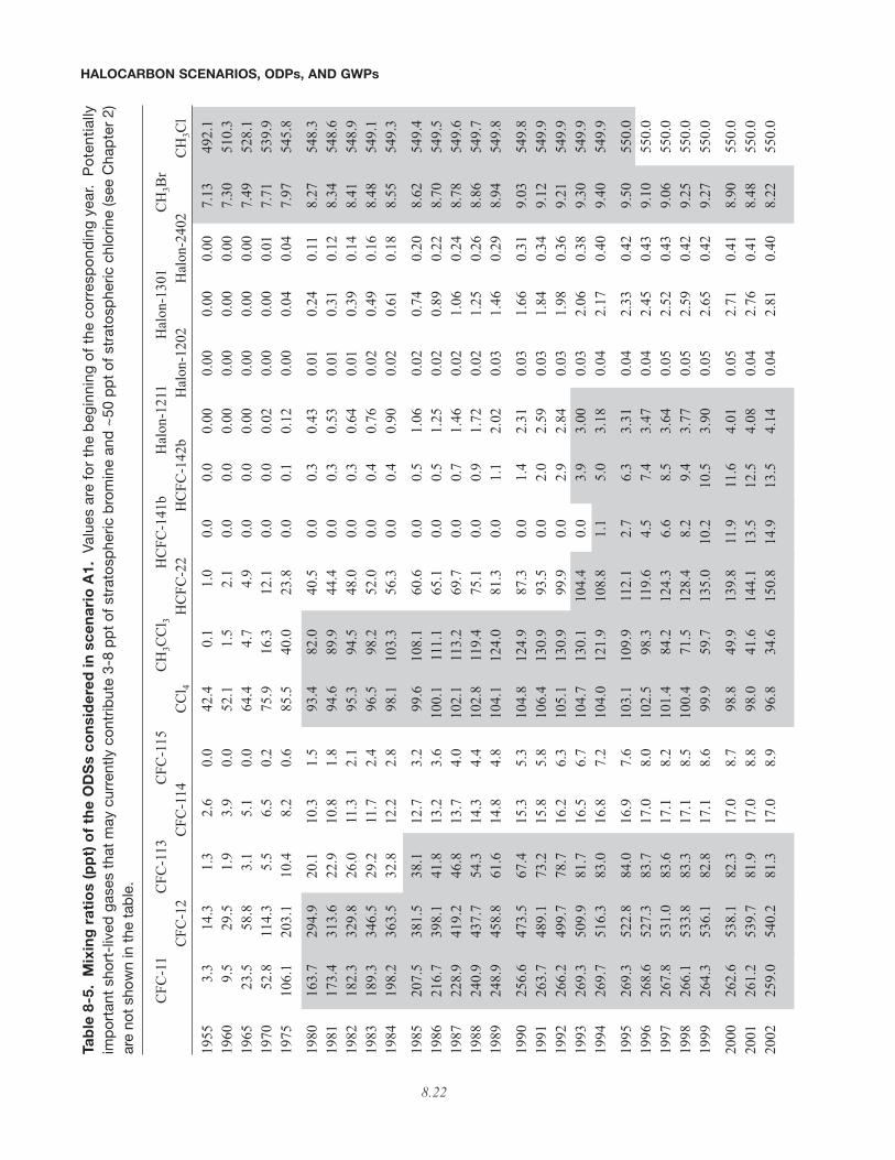
Monitoring Division (ESRL/GMD) (formerly ClimateMonitoring and Diagnostics Laboratory, CMDL)(Montzka et al., 1999) and Advanced Global AtmosphericGases Experiment (AGAGE) networks (Prinn et al., 2005)(and include the University of East Anglia observationsfor halon-1211), and the calibration factors were calcu-lated in a similar manner as in Table 1-15 of WMO (2003).After correcting for calibration differences, the meanmixing ratios of the ESRL/GMD and AGAGE networksare used for temporally overlapping periods for the CFCs,CH3CCl3, and for CCl4. For periods before any overlapexists, the ratios of the measurements are used to extendthe record backward in time in a consistent manner. Theaverage of the December and January observations areassumed to represent the mixing ratios at the start of theyear, with the mixing ratios for the rest of the year calcu-lated from estimated emissions and lifetimes. Althoughthe model is run in 0.1-year time steps, yearly observa-tions are used instead of monthly ones in order to avoidthe impact of seasonal variability on the inferred emis-sions, which are assumed to be constant throughout eachyear. Calculated mixing ratios are tabulated in Table 8-5for each of the considered halocarbons from 1955 through2100. The yearly observations used are indicated in thetable by the shaded regions.
Time series are shown in Figure 8-2 for the currentA1 scenario and the previous Ab scenario. There are somedifferences between mixing ratios of this Assessmentcompared with the previous one for the period 2001-2004,but the greatest differences are found in the future projec-tions. The HCFC-22 projection exhibits the most strikingdifferences compared with the previous Assessment’s sce-nario Ab projection with a peak mixing ratio over 150 ppthigher and peaking more than 20 years later. In contrast,HCFC-141b, HCFC-142b, and halon-1301 exhibitdecreases in near-term projected mixing ratios comparedwith the Ab scenario, due to the decrease in observedgrowth rates from 2001 through 2004 and the expectationof lower future emissions for these species (Figure 8-1).Due to the increased emissions discussed in Section8.3.2.1, future CFC-11 and CFC-12 mixing ratios alsoexhibit modest, but important, increases compared withthe previous Assessment. Carbon tetrachloride decreasesmore slowly in A1 due to greater emission in the comingdecade, with the increased emission based on the uncer-tain source of much of the global CCl4 emission (seeChapter 1) and the slow decline of annual emissions overthe past 15 years.
HALOCARBON SCENARIOS, ODPs, AND GWPs
8.21
HALOCARBON SCENARIOS, ODPs, AND GWPs
8.22
Tab
le 8
-5.
Mix
ing
rat
ios
(pp
t) o
f th
e O
DS
s co
nsi
der
ed in
sce
nar
io A
1. V
alue
s ar
e fo
r th
e b
egin
ning
of
the
corr
esp
ond
ing
yea
r. P
ote
ntia
llyim
por
tant
sho
rt-l
ived
gas
es t
hat
may
cur
rent
ly c
ontr
ibut
e 3-
8 p
pt
of s
trat
osp
heric
bro
min
e an
d ~
50 p
pt
of s
trat
osp
heric
chl
orin
e (s
ee C
hap
ter
2)ar
e no
t sho
wn
in th
e ta
ble
.
CFC
-11
CFC
-113
CFC
-115
CH
3CC
l 3H
CFC
-141
bH
alon
-121
1H
alon
-130
1C
H3B
rC
FC-1
2C
FC-1
14C
Cl 4
HC
FC-2
2H
CFC
-142
bH
alon
-120
2H
alon
-240
2C
H3C
l
1955
3.3
14.3
1.3
2.6
0.0
42.4
0.1
1.0
0.0
0.0
0.00
0.00
0.00
0.00
7.13
492.
119
609.
529
.51.
93.
90.
052
.11.
52.
10.
00.
00.
000.
000.
000.
007.
3051
0.3
1965
23.5
58.8
3.1
5.1
0.0
64.4
4.7
4.9
0.0
0.0
0.00
0.00
0.00
0.00
7.49
528.
119
7052
.811
4.3
5.5
6.5
0.2
75.9
16.3
12.1
0.0
0.0
0.02
0.00
0.00
0.01
7.71
539.
919
7510
6.1
203.
110
.48.
20.
685
.540
.023
.80.
00.
10.
120.
000.
040.
047.
9754
5.8
1980
163.
729
4.9
20.1
10.3
1.5
93.4
82.0
40.5
0.0
0.3
0.43
0.01
0.24
0.11
8.27
548.
319
8117
3.4
313.
622
.910
.81.
894
.689
.944
.40.
00.
30.
530.
010.
310.
128.
3454
8.6
1982
182.
332
9.8
26.0
11.3
2.1
95.3
94.5
48.0
0.0
0.3
0.64
0.01
0.39
0.14
8.41
548.
919
8318
9.3
346.
529
.211
.72.
496
.598
.252
.00.
00.
40.
760.
020.
490.
168.
4854
9.1
1984
198.
236
3.5
32.8
12.2
2.8
98.1
103.
356
.30.
00.
40.
900.
020.
610.
188.
5554
9.3
1985
207.
538
1.5
38.1
12.7
3.2
99.6
108.
160
.60.
00.
51.
060.
020.
740.
208.
6254
9.4
1986
216.
739
8.1
41.8
13.2
3.6
100.
111
1.1
65.1
0.0
0.5
1.25
0.02
0.89
0.22
8.70
549.
519
8722
8.9
419.
246
.813
.74.
010
2.1
113.
269
.70.
00.
71.
460.
021.
060.
248.
7854
9.6
1988
240.
943
7.7
54.3
14.3
4.4
102.
811
9.4
75.1
0.0
0.9
1.72
0.02
1.25
0.26
8.86
549.
719
8924
8.9
458.
861
.614
.84.
810
4.1
124.
081
.30.
01.
12.
020.
031.
460.
298.
9454
9.8
1990
256.
647
3.5
67.4
15.3
5.3
104.
812
4.9
87.3
0.0
1.4
2.31
0.03
1.66
0.31
9.03
549.
819
9126
3.7
489.
173
.215
.85.
810
6.4
130.
993
.50.
02.
02.
590.
031.
840.
349.
1254
9.9
1992
266.
249
9.7
78.7
16.2
6.3
105.
113
0.9
99.9
0.0
2.9
2.84
0.03
1.98
0.36
9.21
549.
919
9326
9.3
509.
981
.716
.56.
710
4.7
130.
110
4.4
0.0
3.9
3.00
0.03
2.06
0.38
9.30
549.
919
9426
9.7
516.
383
.016
.87.
210
4.0
121.
910
8.8
1.1
5.0
3.18
0.04
2.17
0.40
9.40
549.
9
1995
269.
352
2.8
84.0
16.9
7.6
103.
110
9.9
112.
12.
76.
33.
310.
042.
330.
429.
5055
0.0
1996
268.
652
7.3
83.7
17.0
8.0
102.
598
.311
9.6
4.5
7.4
3.47
0.04
2.45
0.43
9.10
550.
019
9726
7.8
531.
083
.617
.18.
210
1.4
84.2
124.
36.
68.
53.
640.
052.
520.
439.
0655
0.0
1998
266.
153
3.8
83.3
17.1
8.5
100.
471
.512
8.4
8.2
9.4
3.77
0.05
2.59
0.42
9.25
550.
019
9926
4.3
536.
182
.817
.18.
699
.959
.713
5.0
10.2
10.5
3.90
0.05
2.65
0.42
9.27
550.
0
2000
262.
653
8.1
82.3
17.0
8.7
98.8
49.9
139.
811
.911
.64.
010.
052.
710.
418.
9055
0.0
2001
261.
253
9.7
81.9
17.0
8.8
98.0
41.6
144.
113
.512
.54.
080.
042.
760.
418.
4855
0.0
2002
259.
054
0.2
81.3
17.0
8.9
96.8
34.6
150.
814
.913
.54.
140.
042.
810.
408.
2255
0.0
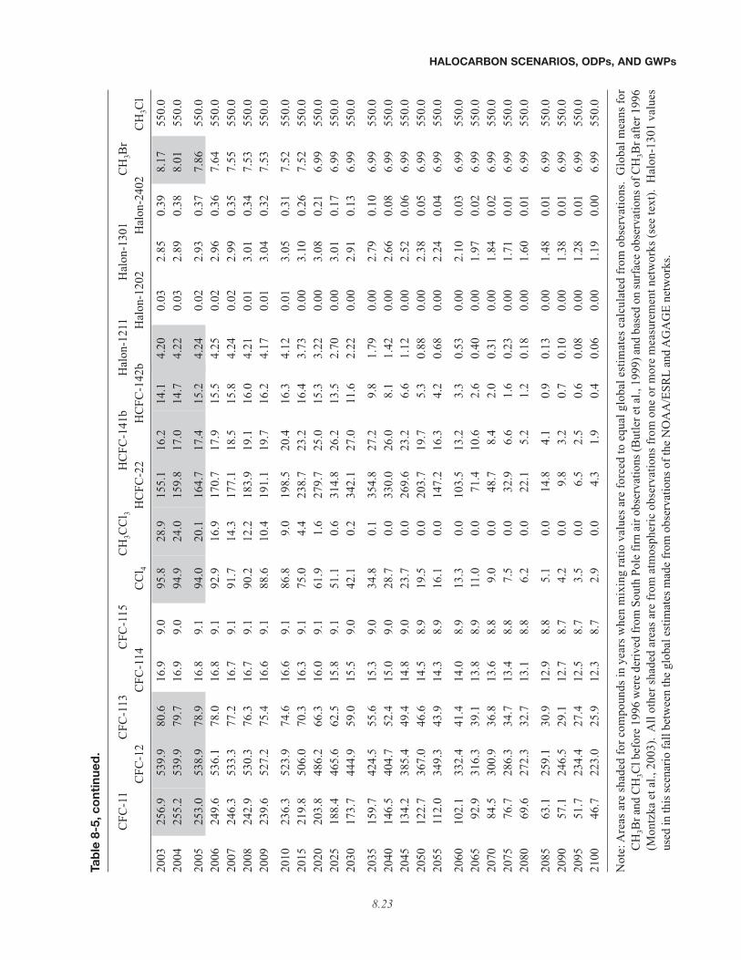
HALOCARBON SCENARIOS, ODPs, AND GWPs
8.23
Tab
le 8
-5, c
ont
inue
d.
CFC
-11
CFC
-113
CFC
-115
CH
3CC
l 3H
CFC
-141
bH
alon
-121
1H
alon
-130
1C
H3B
rC
FC-1
2C
FC-1
14C
Cl 4
HC
FC-2
2H
CFC
-142
bH
alon
-120
2H
alon
-240
2C
H3C
l
2003
256.
953
9.9
80.6
16.9
9.0
95.8
28.9
155.
116
.214
.14.
200.
032.
850.
398.
1755
0.0
2004
255.
253
9.9
79.7
16.9
9.0
94.9
24.0
159.
817
.014
.74.
220.
032.
890.
388.
0155
0.0
2005
253.
053
8.9
78.9
16.8
9.1
94.0
20.1
164.
717
.415
.24.
240.
022.
930.
377.
8655
0.0
2006
249.
653
6.1
78.0
16.8
9.1
92.9
16.9
170.
717
.915
.54.
250.
022.
960.
367.
6455
0.0
2007
246.
353
3.3
77.2
16.7
9.1
91.7
14.3
177.
118
.515
.84.
240.
022.
990.
357.
5555
0.0
2008
242.
953
0.3
76.3
16.7
9.1
90.2
12.2
183.
919
.116
.04.
210.
013.
010.
347.
5355
0.0
2009
239.
652
7.2
75.4
16.6
9.1
88.6
10.4
191.
119
.716
.24.
170.
013.
040.
327.
5355
0.0
2010
236.
352
3.9
74.6
16.6
9.1
86.8
9.0
198.
520
.416
.34.
120.
013.
050.
317.
5255
0.0
2015
219.
850
6.0
70.3
16.3
9.1
75.0
4.4
238.
723
.216
.43.
730.
003.
100.
267.
5255
0.0
2020
203.
848
6.2
66.3
16.0
9.1
61.9
1.6
279.
725
.015
.33.
220.
003.
080.
216.
9955
0.0
2025
188.
446
5.6
62.5
15.8
9.1
51.1
0.6
314.
826
.213
.52.
700.
003.
010.
176.
9955
0.0
2030
173.
744
4.9
59.0
15.5
9.0
42.1
0.2
342.
127
.011
.62.
220.
002.
910.
136.
9955
0.0
2035
159.
742
4.5
55.6
15.3
9.0
34.8
0.1
354.
827
.29.
81.
790.
002.
790.
106.
9955
0.0
2040
146.
540
4.7
52.4
15.0
9.0
28.7
0.0
330.
026
.08.
11.
420.
002.
660.
086.
9955
0.0
2045
134.
238
5.4
49.4
14.8
9.0
23.7
0.0
269.
623
.26.
61.
120.
002.
520.
066.
9955
0.0
2050
122.
736
7.0
46.6
14.5
8.9
19.5
0.0
203.
719
.75.
30.
880.
002.
380.
056.
9955
0.0
2055
112.
034
9.3
43.9
14.3
8.9
16.1
0.0
147.
216
.34.
20.
680.
002.
240.
046.
9955
0.0
2060
102.
133
2.4
41.4
14.0
8.9
13.3
0.0
103.
513
.23.
30.
530.
002.
100.
036.
9955
0.0
2065
92.9
316.
339
.113
.88.
911
.00.
071
.410
.62.
60.
400.
001.
970.
026.
9955
0.0
2070
84.5
300.
936
.813
.68.
89.
00.
048
.78.
42.
00.
310.
001.
840.
026.
9955
0.0
2075
76.7
286.
334
.713
.48.
87.
50.
032
.96.
61.
60.
230.
001.
710.
016.
9955
0.0
2080
69.6
272.
332
.713
.18.
86.
20.
022
.15.
21.
20.
180.
001.
600.
016.
9955
0.0
2085
63.1
259.
130
.912
.98.
85.
10.
014
.84.
10.
90.
130.
001.
480.
016.
9955
0.0
2090
57.1
246.
529
.112
.78.
74.
20.
09.
83.
20.
70.
100.
001.
380.
016.
9955
0.0
2095
51.7
234.
427
.412
.58.
73.
50.
06.
52.
50.
60.
080.
001.
280.
016.
9955
0.0
2100
46.7
223.
025
.912
.38.
72.
90.
04.
31.
90.
40.
060.
001.
190.
006.
9955
0.0
Not
e: A
reas
are
shad
ed fo
r com
poun
ds in
yea
rs w
hen
mix
ing
ratio
val
ues a
re fo
rced
to e
qual
glo
bal e
stim
ates
cal
cula
ted
from
obs
erva
tions
. G
loba
l mea
ns fo
rC
H3B
r and
CH
3Cl b
efor
e 19
96 w
ere
deriv
ed fr
om S
outh
Pol
e fir
n ai
r obs
erva
tions
(But
ler e
t al.,
199
9) a
nd b
ased
on
surf
ace
obse
rvat
ions
of C
H3B
r afte
r 199
6(M
ontz
ka e
t al.,
200
3).
All
othe
r sha
ded
area
s are
from
atm
osph
eric
obs
erva
tions
from
one
or m
ore
mea
sure
men
t net
wor
ks (s
ee te
xt).
Hal
on-1
301
valu
esus
ed in
this
scen
ario
fall
betw
een
the
glob
al e
stim
ates
mad
e fr
om o
bser
vatio
ns o
f the
NO
AA
/ESR
Lan
d A
GA
GE
netw
orks
.
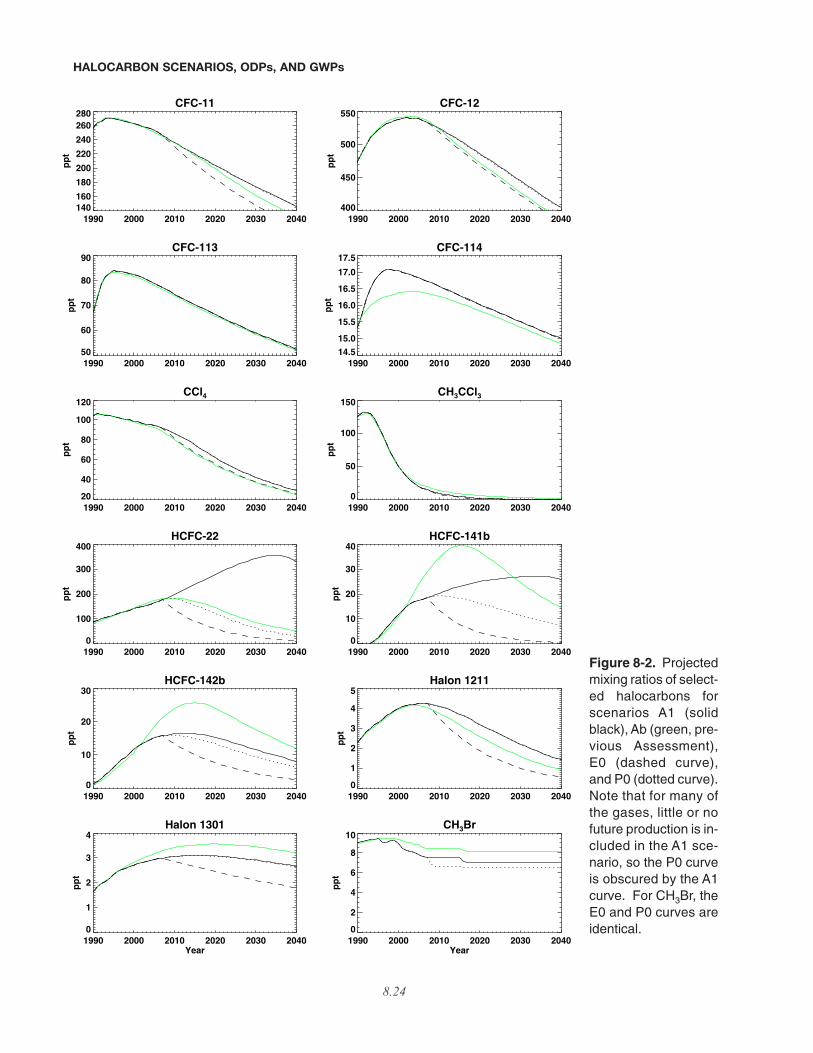
HALOCARBON SCENARIOS, ODPs, AND GWPs
8.24
CFC-11
1990 2000 2010 2020 2030 2040
140160
180
200
220
240
260280
pp
t
CFC-12
1990 2000 2010 2020 2030 2040
400
450
500
550
pp
t
CFC-113
1990 2000 2010 2020 2030 2040
50
60
70
80
90
pp
t
CFC-114
1990 2000 2010 2020 2030 2040
14.5
15.0
15.5
16.0
16.5
17.0
17.5
pp
t
CCl4
1990 2000 2010 2020 2030 2040
20
40
60
80
100
120
pp
t
CH3CCl3
1990 2000 2010 2020 2030 2040
0
50
100
150
pp
t
HCFC-22
1990 2000 2010 2020 2030 2040
0
100
200
300
400
pp
t
HCFC-141b
1990 2000 2010 2020 2030 2040
0
10
20
30
40
pp
t
HCFC-142b
1990 2000 2010 2020 2030 2040
0
10
20
30
pp
t
Halon 1211
1990 2000 2010 2020 2030 2040
0
1
2
3
4
5
pp
t
Halon 1301
1990 2000 2010 2020 2030 2040Year
0
1
2
3
4
pp
t
CH3Br
1990 2000 2010 2020 2030 2040Year
0
2
4
6
8
10
pp
t
Figure 8-2. Projectedmixing ratios of select-ed halocarbons forscenarios A1 (solidblack), Ab (green, pre-vious Assessment),E0 (dashed curve),and P0 (dotted curve).Note that for many ofthe gases, little or nofuture production is in-cluded in the A1 sce-nario, so the P0 curveis obscured by the A1curve. For CH3Br, theE0 and P0 curves areidentical.
8.3.2.3 EQUIVALENT EFFECTIVE STRATOSPHERIC
CHLORINE
The equivalent effective stratospheric chlorine(EESC) index (see Daniel et al., 1995; WMO, 2003) hasbeen used in past Assessments and is summarized in Box8-1. It is used as a measure of the amount of chlorine andbromine available in the stratosphere to destroy ozone.Here, we set fCFC-11, the absolute fractional release value forCFC-11 (Equation 1 of Box 8-1), to be 0.84 as was done inthe previous Assessment, with the ρ values assumed to beequal to the surface mixing ratios. This factor was incor-rectly stated to be 0.8 in footnote “a” of Table 1-4 in the pre-vious Assessment. It should also be noted that the CH3Brmixing ratio at the tropopause may be less than the surfacemixing ratio by a non-negligible amount due to its relativelylarge tropospheric loss (see Chapter 2); this would lead to
an additional reduction in the EESC contribution fromCH3Br that is not considered in this chapter. Newman et al.(2006) have extended the definition of EESC in order for itto correspond to the actual amount of inorganic chlorineand bromine in various stratospheric locations by applyinglocation-appropriate age spectra, fractional release values,and “fCFC-11” values. We do not consider the variation ofEESC with stratospheric location, except in accounting forthe older age of air in the Antarctic polar vortex as discussedbelow. Instead, we continue using EESC as an index thatis only proportional to overall stratospheric inorganic chlo-rine and bromine. Very short-lived species are currently notincluded in the EESC calculation. In the future, as ourknowledge of the very short-lived bromocarbon sourcegases improves (see Chapter 2), it may be warranted tolink EESC directly with spatially varying inorganic chlo-rine and bromine in order to assess the importance of
HALOCARBON SCENARIOS, ODPs, AND GWPs
8.25
Box 8-1. Equivalent Effective Stratospheric Chlorine (EESC)
Due to the established relationship between stratospheric ozone depletion and inorganic chlorine and bromineabundances, the temporal evolution of chlorine- and bromine-containing source gases is an important indicator of thepotential effects of anthropogenic activity on the health of stratospheric ozone. Indices have been developed to demon-strate this halogen evolution in a simple manner. They account for the greater per-atom potency of stratosphericbromine (Br) compared with chlorine (Cl) in its ozone destructiveness with a constant factor, α (Section 8.2.2.3), andinclude the varying rates at which Cl and Br will be released in the stratosphere from different source gases.
EESC provides a simple index that relates the time evolution of long-lived surface abundances of ODSs withthe ozone-destructive ability of stratospheric halogens that come from these long-lived source gases (WMO, 1995,1999, 2003). Contributions of very short-lived chlorine- and bromine-containing sources gases and of troposphericinorganic halogens generally have been neglected. EESC is defined as
(Daniel et al., 1995), where n is the number of chlorine or bromine atoms in the source gas, fi / fCFC-11 represents theefficiency of the stratospheric halogen release relative to that of CFC-11, denoted by fCFC-11 (Section 8.2.2.2), andρi,entry is the tropospheric mixing ratio of source gas i when it entered the stratosphere. Traditionally, ρi,entry is calcu-lated assuming a simple time lag Γ from the surface observations, i.e.,
where ρi (t) is the surface mixing ratio at time t. In WMO (2003), EESC was estimated assuming Γ = 3 years (typicalof the lower, midlatitude stratosphere) to obtain a value appropriate for relating to midlatitude-averaged ozone loss.Effective equivalent chlorine (EECl) (Montzka et al., 1996) is a quantity similar to EESC, but includes no considera-tion of the transport lag time.
To retain the simplicity of the EESC index, several assumptions are generally made in its calculation. One suchassumption is that the stratospheric entry mixing ratio for a given time is taken to be the surface mixing ratio at thattime. This could be an overestimate of the EESC contribution for shorter-lived gases, like CH3Br, whose abundancemay be reduced before reaching the tropopause. In Montzka et al. (2003), this issue has been addressed by reducingthe surface mixing ratio by 7% in the calculation of EESC. A second assumption generally made in EESC calculations
EESC t f nf
fn
f
fCFC ii
CFCi entry i
i
CF
( ) = +−−
1111
ρ α,CC
i entryBr containinghalocarbons
Cl co −−−∑
11
ρ ,nntaining
halocarbons
∑
(1)
ρ ρi entry it t, ( ) = −( )Γ (2)
Continued, next page.
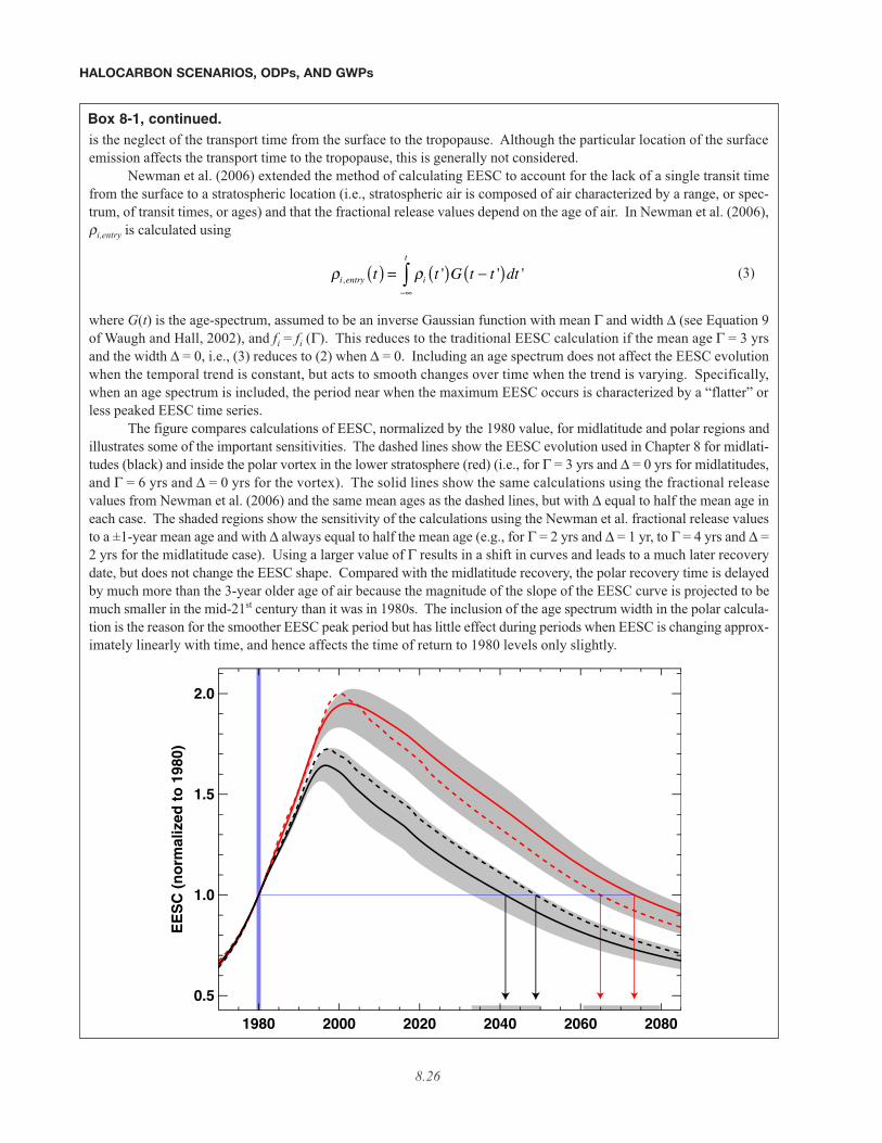
HALOCARBON SCENARIOS, ODPs, AND GWPs
8.26
is the neglect of the transport time from the surface to the tropopause. Although the particular location of the surfaceemission affects the transport time to the tropopause, this is generally not considered.
Newman et al. (2006) extended the method of calculating EESC to account for the lack of a single transit timefrom the surface to a stratospheric location (i.e., stratospheric air is composed of air characterized by a range, or spec-trum, of transit times, or ages) and that the fractional release values depend on the age of air. In Newman et al. (2006),ρi,entry is calculated using
where G(t) is the age-spectrum, assumed to be an inverse Gaussian function with mean Γ and width ∆ (see Equation 9of Waugh and Hall, 2002), and fi = fi (Γ). This reduces to the traditional EESC calculation if the mean age Γ = 3 yrsand the width ∆ = 0, i.e., (3) reduces to (2) when ∆ = 0. Including an age spectrum does not affect the EESC evolutionwhen the temporal trend is constant, but acts to smooth changes over time when the trend is varying. Specifically,when an age spectrum is included, the period near when the maximum EESC occurs is characterized by a “flatter” orless peaked EESC time series.
The figure compares calculations of EESC, normalized by the 1980 value, for midlatitude and polar regions andillustrates some of the important sensitivities. The dashed lines show the EESC evolution used in Chapter 8 for midlati-tudes (black) and inside the polar vortex in the lower stratosphere (red) (i.e., for Γ = 3 yrs and ∆ = 0 yrs for midlatitudes,and Γ = 6 yrs and ∆ = 0 yrs for the vortex). The solid lines show the same calculations using the fractional releasevalues from Newman et al. (2006) and the same mean ages as the dashed lines, but with ∆ equal to half the mean age ineach case. The shaded regions show the sensitivity of the calculations using the Newman et al. fractional release valuesto a ±1-year mean age and with ∆ always equal to half the mean age (e.g., for Γ = 2 yrs and ∆ = 1 yr, to Γ = 4 yrs and ∆ =2 yrs for the midlatitude case). Using a larger value of Γ results in a shift in curves and leads to a much later recoverydate, but does not change the EESC shape. Compared with the midlatitude recovery, the polar recovery time is delayedby much more than the 3-year older age of air because the magnitude of the slope of the EESC curve is projected to bemuch smaller in the mid-21st century than it was in 1980s. The inclusion of the age spectrum width in the polar calcula-tion is the reason for the smoother EESC peak period but has little effect during periods when EESC is changing approx-imately linearly with time, and hence affects the time of return to 1980 levels only slightly.
1980 2000 2020 2040 2060 2080
0.5
1.0
1.5
2.0
EE
SC
(n
orm
aliz
ed t
o 1
980)
(3)ρ ρi entry i
t
t t G t t dt, ' ' '( ) = ( ) −( )−∞∫
Box 8-1, continued.
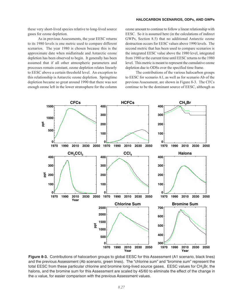
these very short-lived species relative to long-lived sourcegases for ozone depletion.
As in previous Assessments, the year EESC returnsto its 1980 levels is one metric used to compare differentscenarios. The year 1980 is chosen because this is theapproximate date when midlatitude and Antarctic ozonedepletion has been observed to begin. It generally has beenassumed that if all other atmospheric parameters andprocesses remain constant, ozone depletion relates linearlyto EESC above a certain threshold level. An exception tothis relationship is Antarctic ozone depletion. Springtimedepletion became so great around 1990 that there was notenough ozone left in the lower stratosphere for the column
ozone amount to continue to follow a linear relationship withEESC. So it is assumed here (in the calculations of indirectGWPs, Section 8.5) that no additional Antarctic ozonedestruction occurs for EESC values above 1990 levels. Thesecond metric that has been used to compare scenarios isthe integrated EESC value above the 1980 level, integratedfrom 1980 or the current time until EESC returns to the 1980level. This metric is meant to represent the cumulative ozonedepletion due to ODSs over the specified time frame.
The contributions of the various halocarbon groupsto EESC for scenario A1, as well as for scenario Ab of theprevious Assessment, are shown in Figure 8-3. The CFCscontinue to be the dominant source of EESC, although as
HALOCARBON SCENARIOS, ODPs, AND GWPs
8.27
CFCs
1970 1990 2010 2030 2050
0
500
1000
1500
pp
t
HCFCs
1970 1990 2010 2030 2050
0
100
200
300
400
CH3CCl3
1970 1990 2010 2030 2050Year
0
100
200
300
400
pp
t
CCl4
1970 1990 2010 2030 2050
0
100
200
300
400
CH3Br
1970 1990 2010 2030 2050
0
100
200
300
400
Halons
1970 1990 2010 2030 2050
0
100
200
300
400
Chlorine Sum
1970 1990 2010 2030 2050Year
0
500
1000
1500
2000
2500
pp
t
Bromine Sum
1970 1990 2010 2030 2050Year
300
400
500
600
700
Figure 8-3. Contributions of halocarbon groups to global EESC for this Assessment (A1 scenario, black lines)and the previous Assessment (Ab scenario, green lines). The “chlorine sum” and “bromine sum” represent thetotal EESC from these particular chlorine and bromine long-lived source gases. EESC values for CH3Br, thehalons, and the bromine sum for this Assessment are scaled by 45/60 to eliminate the effect of the change inthe α value, for easier comparison with the previous Assessment values.

HALOCARBON SCENARIOS, ODPs, AND GWPs
8.28
a group their contribution has begun to decrease, drivenmostly by the decline of CFC-11. In terms of EESC, themost striking differences between the A1 and Ab sce-narios are the HCFCs. As discussed in Sections 8.3.2.1and 8.3.2.2, this increasing importance of the HCFCs isprimarily due to the increase in expected future produc-tion and emission of HCFC-22 (Table 8-4). The updatesto future emissions of CFCs and HCFCs lead to slightincreases in the importance of these ODS groups to EESCin the future. Updates to the fractional halogen releasevalues of the halons lead to a slightly larger contributionof these compounds. Estimated CH3Br abundances arealso noticeably different from WMO (2003). The differ-ences from 1996 through 2004 arise because of the avail-ability of new global surface data (Montzka et al., 2003,and updates). After that period, differences arise becauseof the larger assumed anthropogenic fraction of CH3Bremission compared with WMO (2003) (30% comparedwith 20%), also based on Montzka et al. (2003). Overall,the updates to the future ODS emissions projections andthe increase in the estimated value for α lead to a later“recovery” of midlatitude-relevant EESC, defined here asa return to pre-1980 values, by about 5 years.
In past Assessments, quantification of midlatitude-relevant EESC was used exclusively. These calculationsassumed a lag of 3 years between surface and stratosphericmixing ratios and assumed a value for α of 45. However,it is known that the age of air in the wintertime polar vortexis greater than 3 years (Andrews et al., 2001; Daniel et al.,1996; Harnisch et al., 1999), and there are indications thatthe value of α should be larger, due to the stronger cou-pling of bromine monoxide (BrO) with chlorine monoxide(ClO) (Chipperfield and Pyle, 1998). Both of these pointsact to delay the halocarbon recovery of the polar vortexcompared with midlatitudes. Consideration of the spec-trum of ages that make up wintertime vortex air can fur-ther delay halocarbon recovery (Newman et al., 2006). Thetime lag increase is expected to be particularly importantbecause of the fast increase in halocarbon abundancesin the 1980s and the relatively slow decline expected inthe future due to halocarbon lifetimes of decades. If atime lag is assumed to be 6 years and a value of α of 65(Chipperfield and Pyle, 1998), the year of EESC recoveryfor Antarctic conditions is 2065, more than 15 years latercompared with the midlatitude EESC recovery; the timelag increase is responsible for almost 13 of the 15 years,with the change in α responsible for the rest. Due to thelarge sensitivity of the EESC recovery to the age of air,all scenarios will be performed for midlatitude-relevantand polar vortex-relevant EESC. Newman et al. (2006)have also shown that the use of a simple lag can lead to
errors in estimated EESC, particularly near the peakperiod. However, because there is little difference in therecovery date when using a simple lag or a more compli-cated age spectrum, and because there is no agreement ona particular globally averaged age spectrum to use, wecontinue to use a simple time lag in this Assessment.
8.3.3 Alternative Projections
8.3.3.1 EMISSIONS
The alternative hypothetical cases used to examinethe relative environmental effects of reducing future pro-duction and emissions of groups of halocarbons are com-pared in Table 8-6 and fall into three categories, each ofwhich is based on the baseline A1 scenario: (1) “no futureemission” cases (E0); (2) “no future production” cases(P0); and (3) cases of the full capture and destruction ofthe 2007 bank (B0). Assumptions of the alternative pro-jections lead to various decreases in future emissions whencompared with the baseline scenario. The hypotheticalelimination of all future emissions (E0) represents thegreatest possible reduction in future abundances. Thehypothetical elimination of future production (P0)allows the ODSs currently residing in banks to continueto be released to the atmosphere as they would in the base-line scenario. The projections that consider the full cap-ture and destruction of the 2007 bank (B0) complementthe “no production” cases in that the full 2007 bank isdestroyed in a manner that releases no ODS to the atmos-phere; future production and the resulting future buildupof banks is allowed to continue, however. This expectedfuture production is small for the CFCs and halons, butsignificant for the HCFCs. A case consistent with the mit-igation scenario presented in IPCC/TEAP (2005) isassessed to illustrate the importance of emissions reduc-tions from this carefully developed scenario on the futureevolution of EESC. The mitigation scenario has a signifi-cant effect only on the banks of HCFC-22, HCFC-123,and HFCs in 2015 (the latter two are not considered in thecases or scenarios of this chapter).
8.3.3.2 MIXING RATIOS
The calculated mixing ratios from 1990 through2040 are shown in Figure 8-2 for the E0 and P0 cases inaddition to the previously discussed A1 and Ab scenarios.These calculations suggest that all ODSs consideredhere, except for the HCFCs and possibly halon-1301 havealready reached their peak mixing ratios. The HCFCs areexpected to reach peak abundances between 2010 and
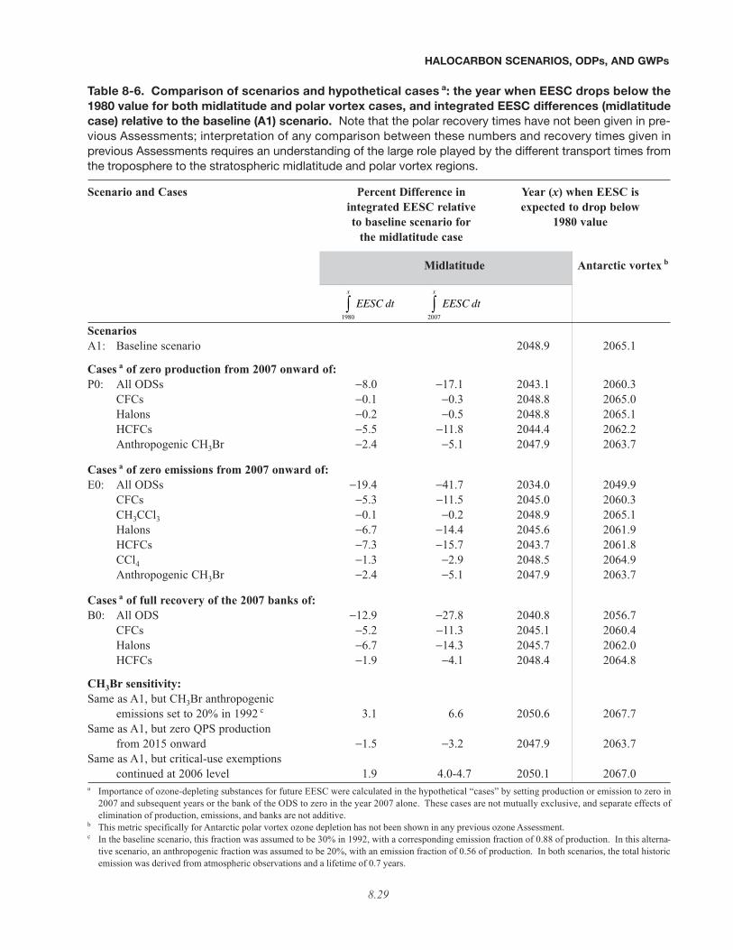
HALOCARBON SCENARIOS, ODPs, AND GWPs
8.29
EESC dtx
1980∫ EESC dt
x
2007∫
Table 8-6. Comparison of scenarios and hypothetical cases a: the year when EESC drops below the1980 value for both midlatitude and polar vortex cases, and integrated EESC differences (midlatitudecase) relative to the baseline (A1) scenario. Note that the polar recovery times have not been given in pre-vious Assessments; interpretation of any comparison between these numbers and recovery times given inprevious Assessments requires an understanding of the large role played by the different transport times fromthe troposphere to the stratospheric midlatitude and polar vortex regions.
Scenario and Cases Percent Difference in Year (x) when EESC isintegrated EESC relative expected to drop belowto baseline scenario for 1980 value
the midlatitude case
Midlatitude Antarctic vortex b
ScenariosA1: Baseline scenario 2048.9 2065.1
Cases a of zero production from 2007 onward of:P0: All ODSs −8.0 −17.1 2043.1 2060.3
CFCs −0.1 −0.3 2048.8 2065.0Halons −0.2 −0.5 2048.8 2065.1HCFCs −5.5 −11.8 2044.4 2062.2Anthropogenic CH3Br −2.4 −5.1 2047.9 2063.7
Cases a of zero emissions from 2007 onward of:E0: All ODSs −19.4 −41.7 2034.0 2049.9
CFCs −5.3 −11.5 2045.0 2060.3CH3CCl3 −0.1 −0.2 2048.9 2065.1Halons −6.7 −14.4 2045.6 2061.9HCFCs −7.3 −15.7 2043.7 2061.8CCl4 −1.3 −2.9 2048.5 2064.9Anthropogenic CH3Br −2.4 −5.1 2047.9 2063.7
Cases a of full recovery of the 2007 banks of:B0: All ODS −12.9 −27.8 2040.8 2056.7
CFCs −5.2 −11.3 2045.1 2060.4Halons −6.7 −14.3 2045.7 2062.0HCFCs −1.9 −4.1 2048.4 2064.8
CH3Br sensitivity:Same as A1, but CH3Br anthropogenic
emissions set to 20% in 1992 c 3.1 6.6 2050.6 2067.7Same as A1, but zero QPS production
from 2015 onward −1.5 −3.2 2047.9 2063.7Same as A1, but critical-use exemptions
continued at 2006 level 1.9 4.0-4.7 2050.1 2067.0a Importance of ozone-depleting substances for future EESC were calculated in the hypothetical “cases” by setting production or emission to zero in
2007 and subsequent years or the bank of the ODS to zero in the year 2007 alone. These cases are not mutually exclusive, and separate effects ofelimination of production, emissions, and banks are not additive.
b This metric specifically for Antarctic polar vortex ozone depletion has not been shown in any previous ozone Assessment.c In the baseline scenario, this fraction was assumed to be 30% in 1992, with a corresponding emission fraction of 0.88 of production. In this alterna-
tive scenario, an anthropogenic fraction was assumed to be 20%, with an emission fraction of 0.56 of production. In both scenarios, the total historicemission was derived from atmospheric observations and a lifetime of 0.7 years.
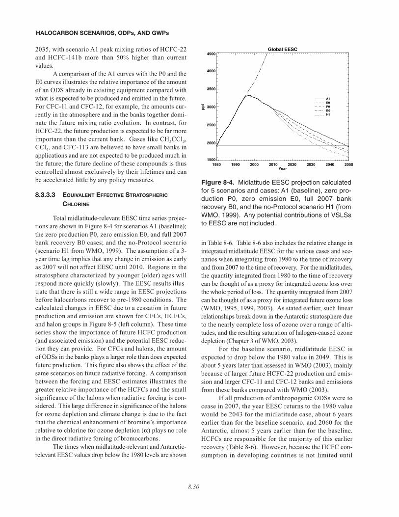
2035, with scenario A1 peak mixing ratios of HCFC-22and HCFC-141b more than 50% higher than currentvalues.
A comparison of the A1 curves with the P0 and theE0 curves illustrates the relative importance of the amountof an ODS already in existing equipment compared withwhat is expected to be produced and emitted in the future.For CFC-11 and CFC-12, for example, the amounts cur-rently in the atmosphere and in the banks together domi-nate the future mixing ratio evolution. In contrast, forHCFC-22, the future production is expected to be far moreimportant than the current bank. Gases like CH3CCl3,CCl4, and CFC-113 are believed to have small banks inapplications and are not expected to be produced much inthe future; the future decline of these compounds is thuscontrolled almost exclusively by their lifetimes and canbe accelerated little by any policy measures.
8.3.3.3 EQUIVALENT EFFECTIVE STRATOSPHERIC
CHLORINE
Total midlatitude-relevant EESC time series projec-tions are shown in Figure 8-4 for scenarios A1 (baseline);the zero production P0, zero emission E0, and full 2007bank recovery B0 cases; and the no-Protocol scenario(scenario H1 from WMO, 1999). The assumption of a 3-year time lag implies that any change in emission as earlyas 2007 will not affect EESC until 2010. Regions in thestratosphere characterized by younger (older) ages willrespond more quickly (slowly). The EESC results illus-trate that there is still a wide range in EESC projectionsbefore halocarbons recover to pre-1980 conditions. Thecalculated changes in EESC due to a cessation in futureproduction and emission are shown for CFCs, HCFCs,and halon groups in Figure 8-5 (left column). These timeseries show the importance of future HCFC production(and associated emission) and the potential EESC reduc-tion they can provide. For CFCs and halons, the amountof ODSs in the banks plays a larger role than does expectedfuture production. This figure also shows the effect of thesame scenarios on future radiative forcing. A comparisonbetween the forcing and EESC estimates illustrates thegreater relative importance of the HCFCs and the smallsignificance of the halons when radiative forcing is con-sidered. This large difference in significance of the halonsfor ozone depletion and climate change is due to the factthat the chemical enhancement of bromine’s importancerelative to chlorine for ozone depletion (α) plays no rolein the direct radiative forcing of bromocarbons.
The times when midlatitude-relevant and Antarctic-relevant EESC values drop below the 1980 levels are shown
in Table 8-6. Table 8-6 also includes the relative change inintegrated midlatitude EESC for the various cases and sce-narios when integrating from 1980 to the time of recoveryand from 2007 to the time of recovery. For the midlatitudes,the quantity integrated from 1980 to the time of recoverycan be thought of as a proxy for integrated ozone loss overthe whole period of loss. The quantity integrated from 2007can be thought of as a proxy for integrated future ozone loss(WMO, 1995, 1999, 2003). As stated earlier, such linearrelationships break down in the Antarctic stratosphere dueto the nearly complete loss of ozone over a range of alti-tudes, and the resulting saturation of halogen-caused ozonedepletion (Chapter 3 of WMO, 2003).
For the baseline scenario, midlatitude EESC isexpected to drop below the 1980 value in 2049. This isabout 5 years later than assessed in WMO (2003), mainlybecause of larger future HCFC-22 production and emis-sion and larger CFC-11 and CFC-12 banks and emissionsfrom these banks compared with WMO (2003).
If all production of anthropogenic ODSs were tocease in 2007, the year EESC returns to the 1980 valuewould be 2043 for the midlatitude case, about 6 yearsearlier than for the baseline scenario, and 2060 for theAntarctic, almost 5 years earlier than for the baseline.HCFCs are responsible for the majority of this earlierrecovery (Table 8-6). However, because the HCFC con-sumption in developing countries is not limited until
HALOCARBON SCENARIOS, ODPs, AND GWPs
8.30
Global EESC
1980 1990 2000 2010 2020 2030 2040 2050Year
1500
2000
2500
3000
3500
4000
4500
pp
t
A1E0P0B0H1
Figure 8-4. Midlatitude EESC projection calculatedfor 5 scenarios and cases: A1 (baseline), zero pro-duction P0, zero emission E0, full 2007 bankrecovery B0, and the no-Protocol scenario H1 (fromWMO, 1999). Any potential contributions of VSLSsto EESC are not included.
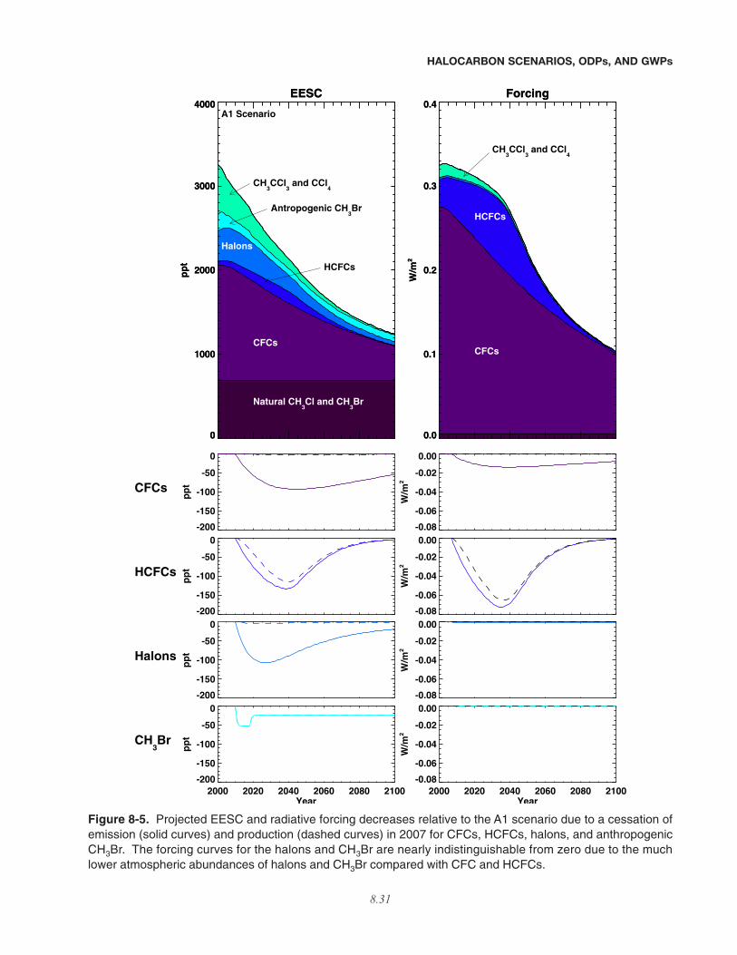
HALOCARBON SCENARIOS, ODPs, AND GWPs
8.31
-200
-150
-100
-50
0
pp
tCFCs
-0.08
-0.06
-0.04
-0.02
0.00
W/m
2
-200
-150
-100
-50
0
pp
tHCFCs
-0.08
-0.06
-0.04
-0.02
0.00
W/m
2
-200
-150
-100
-50
0
pp
tHalons
-0.08
-0.06
-0.04
-0.02
0.00
W/m
2
2000 2020 2040 2060 2080 2100Year
-200
-150
-100
-50
0
pp
tCH3Br
2000 2020 2040 2060 2080 2100Year
-0.08
-0.06
-0.04
-0.02
0.00
W/m
2
EESC
0
1000
2000
3000
4000
pp
t
EESC
0
1000
2000
3000
4000
pp
t
Natural CH3Cl and CH
3Br
CFCs
Halons
HCFCs
CH3CCl
3 and CCl
4
Antropogenic CH3Br
A1 Scenario
Forcing
0.0
0.1
0.2
0.3
0.4
W/m
2
CFCs
HCFCs
CH3CCl
3 and CCl
4
Forcing
0.0
0.1
0.2
0.3
0.4
W/m
2
Figure 8-5. Projected EESC and radiative forcing decreases relative to the A1 scenario due to a cessation ofemission (solid curves) and production (dashed curves) in 2007 for CFCs, HCFCs, halons, and anthropogenicCH3Br. The forcing curves for the halons and CH3Br are nearly indistinguishable from zero due to the muchlower atmospheric abundances of halons and CH3Br compared with CFC and HCFCs.
2015, the assumptions regarding this consumption in theA1 scenario largely determine the magnitude of this ear-lier recovery. Smaller contributions come from the futureproduction of CFCs, halons, and methyl bromide.
In the hypothetical case in which all anthropogenicemissions of ODSs were to cease in 2007, the futuremixing ratios and EESC are governed entirely by the nat-ural destruction in the atmosphere (and ocean/soil) of theODSs. In this case the midlatitude EESC would dropbelow the 1980 value in 2034. The largest contributionsto the zero emission cases come from HCFCs (especiallyHCFC-22), CFCs, and halons.
In the hypothetical case that the 2007 bank of CFCs,halons, and HCFCs were fully recovered and preventedfrom being emitted into the atmosphere, EESC would dropbelow the 1980 value 4, 3, and 0.5 years earlier, respec-tively, compared with the baseline scenario.
In the IPCC (IPCC/TEAP, 2005) “mitigation” sce-nario, economic, and technological analyses were per-formed in an attempt to determine reasonable reductionsin future ODS emissions that could be accomplishedusing current best-practice emission reduction tech-niques. The mitigation scenario shows a decrease from1879 to 1587 ktons in the bank of HCFC-22 in 2015. Thisdecrease in the bank leads to a reduced emission over theperiod 2007-2050 from 15 to 11 Mt, contributing to anODP-weighted decrease of the HCFCs from 1.0 to 0.8 Mt.The emission reduction in the mitigation scenario corre-sponds thereby to about 20% of the zero-emissions caseof the HCFCs. Hence, the effects of the mitigation sce-nario, in terms of the length of time required for the ODSsto return to 1980 levels and the integrated EESC abovethe 1980 level, are also about 20% of the effects of thezero emissions case of the HCFCs (Table 8-6).
A few additional cases have been assessed formethyl bromide. There is uncertainty (see Section 1.2.1.7)regarding the fraction of anthropogenic emissions thatcomprise the sources needed to balance the sinks that arebased on the observed surface mixing ratio and a globallifetime of 0.7 years. Montzka et al. (1999) estimated thatthe emission of CH3Br resulting from industrial produc-tion is between 10% and 40% of the total emission in 1992.In the baseline scenario, this fraction is assumed to be 30%,higher than assumed in WMO (2003), but consistent withthe discussions in Chapter 1. As a sensitivity study, ananthropogenic fraction of 20% was assumed in an alterna-tive scenario. In our calculations, this 20% fraction is con-sistent with an emission fraction of 0.56 of the industrialproduction, meaning that 56% of the industrially producedCH3Br is emitted to the atmosphere. This is, in turn, con-sistent with the range of 0.43-0.87 from agricultural andrelated uses as reported by UNEP (1998). The magnitude
of natural emissions for this case is 165 ktons, comparedwith 146 ktons in scenario A1, and compared with a totalanthropogenic production of 73 ktons in 1992. In thisalternative scenario, EESC drops below the 1980 valuealmost 2 years later than in the baseline scenario, demon-strating the expected effect of a smaller significance ofanthropogenic CH3Br emission reductions in a case inwhich natural emission plays a larger role.
A complete phase-out (except for critical and non-regulated uses) of the production and consumption ofmethyl bromide in developed countries (non-Article5(1)) came into effect in 2005. Several countries haveasked and obtained exemptions for critical uses of methylbromide. In 2005, these exemptions totaled about 14ktons and in 2006 about 13 ktons, which is 50-60% ofthe reported production in 2003-2004. In the baselinescenario, it is assumed that the critical-use exemptionscontinue at the 2006 level until 2015, when they are nolonger granted and production in Article 5(1) countriesis terminated. The existence of possible stockpiles ofmethyl bromide is not taken into account in the scenarios.If critical-use exemptions continue indefinitely at the2006 level compared with a cessation of these exemp-tions in 2010 or 2015, midlatitude integrated EESCwould increase by 4.7% or 4.0%, respectively.
Production of methyl bromide for quarantine andpre-shipment (QPS) is not controlled by the MontrealProtocol. In the baseline scenario, the QPS production,estimated at 10.7 ktons per year, is continued indefi-nitely. If the QPS production were to cease in 2015, theyear EESC is expected to drop below the 1980 value isabout a year earlier. This effect depends on the assump-tion of constant QPS emissions in the future in the base-line scenario and would be different if an alternativefuture QPS emission assumption were made. The esti-mated emissions of QPS are close to those of the crit-ical-use exemptions and they have consequently similarcontributions to the integrated EESC.
8.3.4 Uncertainties in ODS Projections
Numerous processes can affect the amount of ozoneloss for a given halogen loading level. Many of these havebeen discussed in Chapters 5 and 6, and some will be men-tioned in Section 8.4. Here we will focus on the uncer-tainties in the ODS projections themselves. Unfortunately,little work has been performed in this area, leading to amostly qualitative assessment of the sensitivities of theprojections presented here.
Before future emission projections based on thebottom-up analyses considered here can be considered fullyreliable, the causes of the discrepancies with the top-down
HALOCARBON SCENARIOS, ODPs, AND GWPs
8.32

estimates need to be better understood. Whether themissing emission from the bottom-up analysis is due tofaster release from the bank than estimated, additionalpast production that has led to a larger bank and a corre-spondingly higher bank release, additional production andimmediate release from use as solvent or aerosol propel-lant, or another factor, the particular assumptions made canlead to important differences in future ODS projections. Ameasure of the sensitivity of a particular gas’s mixing ratioprojection to the size of the bank, compared with futureproduction uncertainties, can be obtained from Figures 8-2and 8-5. For example, CFC-11 and the CFC group willhave more sensitivity to uncertainties in the size of its bank,while HCFC-22 and the HCFC group will have more sen-sitivity to uncertainties in future production. While it isimportant to recognize the large emission discrepanciesbetween these bottom-up analysis and observations for afew species, it is also important to consider the species thatdemonstrate relatively good agreement with emissions(CFC-12, HCFC-22, and halon-1211). Even for thesespecies, there are important differences in the sizes of theestimated bank, depending on the method used to estimatethis quantity. Table 8-7 shows a comparison of bank esti-mates from this Assessment, the previous Assessment(WMO, 2003), and IPCC/TEAP (2005). The large discrep-ancies between the CFC-11 and CFC-12 banks have beenshown by Daniel et al. (2006) to have important implica-tions for estimating the benefit of recycling/destroying theCFC banks. While the banks are calculated in thisAssessment in a manner to agree best with the IPCC/TEAP(2005) estimates for many of the considered ODSs, thecause of this discrepancy has not been resolved.
Another potential explanation for some of the banksize discrepancy could be due to an error in the assumedfactor of 1.07 that relates the surface mixing ratio to theglobally averaged mixing ratio. A higher (lower) valuefor this factor would lead to smaller (larger) emissionsestimated from atmospheric mixing ratio observations,and thus to larger (smaller) top-down bank sizes. Danielet al. (2006) found, for example, that an increase in thisfactor to 1.10 from 1.07 would lead to an additionalamount of banked CFC-11 in 2002 of 250 ktons, repre-senting about 20% of the difference between the top-downestimate of WMO (2003) and the bottom-up estimate ofIPCC/TEAP (2005).
Changes in atmospheric lifetimes, whether due tochanging atmospheric dynamics or chemistry, can alsoaffect future ODS projections. The recently published sug-gestion of an important soil sink that could reduce thecarbon tetrachloride lifetime from 26 to 20 years (Happelland Roche, 2003), and its resulting implications for aquicker recovery of EESC to 1980 values, is one example
of the importance of lifetime uncertainties. Daniel et al.(2006) have shown that an increase in the CFC-11 lifetimeby 10% would result in reduced annual emissions requiredto be consistent with observed mixing ratios that wouldlead to an increase in the 2002 bank by 300 ktons. The12-box model emission estimates discussed in Section8.3.2.1 can presumably account for changes in global life-times due to changing atmospheric distributions, as wellas changes in the factor relating surface mixing ratio tothe global mixing ratio average, better than the 1-boxmodel. These differences likely play a role in the higheremissions estimates of the 12-box model (Section 8.3.2.1);however, these higher emissions would lead to smallerbank estimates using the top-down formalism in thischapter, and thus to even larger bank size discrepancieswith the bottom-up analysis.
The release rate applied to the particular usagebanks can affect the accuracy of future ODS projections.For example, there is a question as to how quickly ODSsare released from foam insulation once it is sent to a land-fill (IPCC/TEAP, 2005). If foam ODSs were not releasedfor 40 years, recycling these particular ODSs would havea much reduced benefit than if release were much sooner.This results because by the time the ODS would be finallyreleased in the absence of recycling, EESC would havealmost returned to pre-1980 levels in extrapolar regions ofthe lower stratosphere.
Sources of uncertainty in relating tropospheric mix-ing ratios to EESC include location- and time-dependentfractional chlorine/bromine release, age of air, and, α values.
HALOCARBON SCENARIOS, ODPs, AND GWPs
8.33
Table 8-7. Comparison of halocarbon banks(ktons) in 2002 used in this Assessment, the pre-vious Assessment (WMO, 2003), and IPCC/TEAP(2005).
Species WMO (2003) IPCC/TEAP This2002 Bank (2005) Assessment
2002 Bank 2002 Bank
CFC-11 594 1,687 1,654CFC-12 0 711 711CFC-113 7 0 5HCFC-22 1,317 1,531 1,531HCFC-141b 753 836 674HCFC-142b 210 224 224Halon-1211 72 125 125Halon-1301 58 42 42CH3CCl3 530 ** Production and bank were not estimated; we assume emissions are
equal to production, implying a zero bank. Protocol limitations areplaced directly on emissions.
We have given examples of the potential significance of ageof air and α variations, but there have been no studies exam-ining the importance of the fractional halogen release varia-tions with location. To the extent that much of the ozonedepletion occurs in the lower stratosphere, where the releasevalues remain relatively constant with location (Solomon etal., 1992), it has generally been assumed that any variabilitywould represent a minor effect. The fractional chlorinerelease values of HCFC-141b and HCFC-142b representtwo cases in which there is significant uncertainty regard-ing the correct value. The previous Assessment discussedthe large differences between the previously assumedmodel-derived values and the values estimated from obser-vations (Schauffler et al., 2003). The model-derived valueswere retained because of the large importance of the age-of-air correction in interpreting observations of gaseswith such a large growth rate. However, it is unlikely thatthe age-of-air correction could be responsible for such alarge discrepancy. Unfortunately, no work has been per-formed since the previous Assessment to resolve thesequestions. Therefore, we continue to use the same valuesthat were used in the previous Assessment, but caution thatthese values could be too large. While the ODPs of HCFC-141b and -142b are much larger than the ODP of HCFC-22, the effect of this fractional chlorine release uncertaintyis limited by the lower projected mixing ratios of thesetwo HCFCs compared with HCFC-22 (Figure 8-2). Never-theless, uncertainties in the fractional release values formany of the ODSs do represent an important uncertainty inEESC calculations. These release values affect the relativeimportance of certain ODSs to total EESC and can thusaffect future EESC evolution. If, for example, the Schauffleret al. release values (2- to 4.5-year means) were used insteadof the ones assumed in this chapter, the EESC return to 1980levels would occur about 3 years earlier.
It is important to recognize that errors in the accu-rate modeling of the baseline scenario can translatedirectly into errors in interpreting the alternative scenariosand test cases. For example, an error in the value of αwill lead directly to an error in the assessment of the zeroemission and production test cases for reducing EESC,particularly for the bromocarbons. As another example,any unreasonable assumption in the baseline scenario forfuture production of any species will necessarily affectthe conclusions derived from both the “no production”and “no emission” test cases.
8.4 OTHER PROCESSES RELEVANT TOFUTURE OZONE EVOLUTION
To enable policy-relevant discussion of future sce-narios, this chapter has made several simplifying assump-
tions. This chapter characterizes the complexities ofozone depletion using simple parameterizations based onODPs. But perhaps more important, the scenarios areassumed to evolve within an unchanging backgroundstate. Given projections of climate change (e.g., IPCC,2001), and our understanding of ozone and climate inter-actions (WMO, 2003; IPCC/TEAP, 2005; Chapter 5 andChapter 6), this assumption is known to be inaccurate.This section qualitatively discusses a few possible conse-quences of a changing background state on the relation-ship between ODS emissions, EESC, and stratosphericozone depletion. More details regarding the effects ofclimate change on the future ozone evolution can be foundin Chapters 5 and 6.
Both natural and anthropogenic forcings of climatechange have the potential to alter important chemistryrelated to future stratospheric ozone depletion for a givenfuture evolution of ODSs and EESC. Two primary nat-ural forcing mechanisms include solar changes and vol-canic eruptions. Currently, solar changes are not expectedto have a long-term effect on ozone recovery. However, avolcanic eruption that injects a large amount of sulfateaerosols into the stratosphere in the next few decades mayenhance halogen ozone destruction. While this shouldperturb ozone chemistry for only a few years, the pertur-bations during that time could be substantial.
Future anthropogenic emissions of gases likecarbon dioxide (CO2), nitrous oxide (N2O), and methane(CH4) will also affect the chemical response of ozonedepletion to ODS emissions and EESC. The expectedstratospheric cooling induced by increasing concentra-tions, primarily of CO2, is expected to slow gas-phaseozone depletion reactions and increase global ozone;conversely, polar springtime ozone could be reduced bycooler temperatures and the resulting increase in hetero-geneous ozone loss. The expected future increase inN2O will increase stratospheric NOx, which is expectedto exacerbate globally averaged ozone depletion. How-ever, increases in CH4 abundances could accelerateozone recovery. Hence, the globally averaged net effectof increases in these two important trace species dependson the specific future emission scenario. Emissions ofhydrocarbons and NOx are also expected to affect thelifetime and concentrations of stratospheric sourcegases, such as HCFCs, CH3Br, CH3Cl, and CH4, andthereby affect ozone.
Climate change by any cause (human, natural, orvariability) can also be expected to affect atmosphericdynamics, which could lead to changes in ozone. Thesechanges could be due, for example, to changes in thetransport of ozone itself, or to changes in the lifetimes ofthe source gases.
HALOCARBON SCENARIOS, ODPs, AND GWPs
8.34
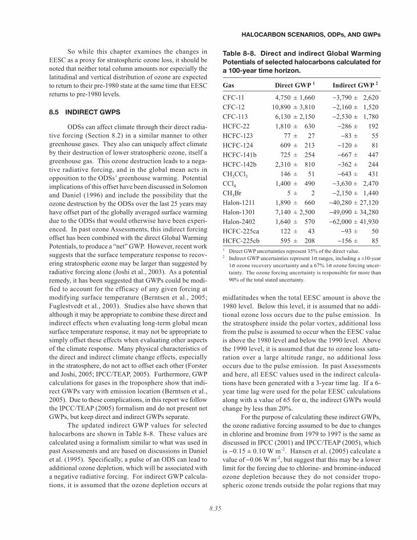
So while this chapter examines the changes inEESC as a proxy for stratospheric ozone loss, it should benoted that neither total column amounts nor especially thelatitudinal and vertical distribution of ozone are expectedto return to their pre-1980 state at the same time that EESCreturns to pre-1980 levels.
8.5 INDIRECT GWPS
ODSs can affect climate through their direct radia-tive forcing (Section 8.2) in a similar manner to othergreenhouse gases. They also can uniquely affect climateby their destruction of lower stratospheric ozone, itself agreenhouse gas. This ozone destruction leads to a nega-tive radiative forcing, and in the global mean acts inopposition to the ODSs’ greenhouse warming. Potentialimplications of this offset have been discussed in Solomonand Daniel (1996) and include the possibility that theozone destruction by the ODSs over the last 25 years mayhave offset part of the globally averaged surface warmingdue to the ODSs that would otherwise have been experi-enced. In past ozone Assessments, this indirect forcingoffset has been combined with the direct Global WarmingPotentials, to produce a “net” GWP. However, recent worksuggests that the surface temperature response to recov-ering stratospheric ozone may be larger than suggested byradiative forcing alone (Joshi et al., 2003). As a potentialremedy, it has been suggested that GWPs could be modi-fied to account for the efficacy of any given forcing atmodifying surface temperature (Berntsen et al., 2005;Fuglestvedt et al., 2003). Studies also have shown thatalthough it may be appropriate to combine these direct andindirect effects when evaluating long-term global meansurface temperature response, it may not be appropriate tosimply offset these effects when evaluating other aspectsof the climate response. Many physical characteristics ofthe direct and indirect climate change effects, especiallyin the stratosphere, do not act to offset each other (Forsterand Joshi, 2005; IPCC/TEAP, 2005). Furthermore, GWPcalculations for gases in the troposphere show that indi-rect GWPs vary with emission location (Berntsen et al.,2005). Due to these complications, in this report we followthe IPCC/TEAP (2005) formalism and do not present netGWPs, but keep direct and indirect GWPs separate.
The updated indirect GWP values for selectedhalocarbons are shown in Table 8-8. These values arecalculated using a formalism similar to what was used inpast Assessments and are based on discussions in Danielet al. (1995). Specifically, a pulse of an ODS can lead toadditional ozone depletion, which will be associated witha negative radiative forcing. For indirect GWP calcula-tions, it is assumed that the ozone depletion occurs at
midlatitudes when the total EESC amount is above the1980 level. Below this level, it is assumed that no addi-tional ozone loss occurs due to the pulse emission. Inthe stratosphere inside the polar vortex, additional lossfrom the pulse is assumed to occur when the EESC valueis above the 1980 level and below the 1990 level. Abovethe 1990 level, it is assumed that due to ozone loss satu-ration over a large altitude range, no additional lossoccurs due to the pulse emission. In past Assessmentsand here, all EESC values used in the indirect calcula-tions have been generated with a 3-year time lag. If a 6-year time lag were used for the polar EESC calculationsalong with a value of 65 for α, the indirect GWPs wouldchange by less than 20%.
For the purpose of calculating these indirect GWPs,the ozone radiative forcing assumed to be due to changesin chlorine and bromine from 1979 to 1997 is the same asdiscussed in IPCC (2001) and IPCC/TEAP (2005), whichis −0.15 ± 0.10 W m-2. Hansen et al. (2005) calculate avalue of −0.06 W m-2, but suggest that this may be a lowerlimit for the forcing due to chlorine- and bromine-inducedozone depletion because they do not consider tropo-spheric ozone trends outside the polar regions that may
HALOCARBON SCENARIOS, ODPs, AND GWPs
8.35
Table 8-8. Direct and indirect Global WarmingPotentials of selected halocarbons calculated fora 100-year time horizon.
Gas Direct GWP 1 Indirect GWP 2
CFC-11 4,750 ± 1,660 −3,790 ± 2,620CFC-12 10,890 ± 3,810 −2,160 ± 1,520CFC-113 6,130 ± 2,150 −2,530 ± 1,780HCFC-22 1,810 ± 630 −286 ± 192HCFC-123 77 ± 27 −83 ± 55HCFC-124 609 ± 213 −120 ± 81HCFC-141b 725 ± 254 −667 ± 447HCFC-142b 2,310 ± 810 −362 ± 244CH3CCl3 146 ± 51 −643 ± 431CCl4 1,400 ± 490 −3,630 ± 2,470CH3Br 5 ± 2 −2,150 ± 1,440Halon-1211 1,890 ± 660 −40,280 ± 27,120Halon-1301 7,140 ± 2,500 −49,090 ± 34,280Halon-2402 1,640 ± 570 −62,000 ± 41,930HCFC-225ca 122 ± 43 −93 ± 50HCFC-225cb 595 ± 208 −156 ± 851 Direct GWP uncertainties represent 35% of the direct value.2 Indirect GWP uncertainties represent 1σ ranges, including a ±10-year
1σ ozone recovery uncertainty and a 67% 1σ ozone forcing uncer-tainty. The ozone forcing uncertainty is responsible for more than90% of the total stated uncertainty.
have arisen due to chlorine and bromine changes. A recentstudy that compares model calculations of ozone changessince preindustrial times suggests a range of −0.123 to+0.066 W m-2 for the forcing due to stratospheric ozonechanges through the year 2000, when climate changes areneglected (Gauss et al., 2006). However, we have chosento retain the previous forcing estimate because the Gausset al. (2006) study does not quantify the mitigating forc-ing effects of tropospheric ozone and ozone precursorincreases on stratospheric ozone, particularly in the lowerstratosphere, where ozone changes are so important toradiative forcing calculations. It would be inappropriateto include the effect of tropospheric ozone chemistry notdue to halogens in the indirect GWP estimates of chloro-carbons and bromocarbons.
The differences between the indirect GWP esti-mates in Table 8-8 and those in WMO (2003) (net GWPsminus direct GWPs of Table 1-8) are attributable to: anew ODS scenario that leads to a return to pre-1980 levelsof EESC later; an updated CO2 mixing ratio; a new CO2pulse response function; a change in the year of emis-sion from 2002 to 2007; the updated value of α; and dif-ferent fractional bromine release values that are nowconsistent with Table 8-1 (and Table 1-4 in WMO, 2003)rather than the values used for CH3Br, halon-1211, andhalon-1301 of 1.08, 1.1, and 0.8, respectively, used inTable 1-8 of WMO (2003). Differences compared withIPCC/TEAP (2005) are due to the updated CO2 mixingratio and response function, to the new ODS scenario, andto the different value of α.
The direct GWP uncertainties represent 35% of thedirect GWP values, consistent with Section 8.2.3. Theindirect uncertainties represent a 1σ uncertainty due to a±10-year 1σ error in the year of EESC recovery to 1980levels and a 67% 1σ uncertainty in the ozone radiativeforcing; this ozone forcing uncertainty accounts for nearlyall of the quoted uncertainty total. It should be noted thatthese errors associated with GWPs are in addition to thepotentially large difference in climate sensitivity (i.e., theamount of temperature change per change in radiativeforcing, dT/dF) between stratospheric ozone loss and thewell-mixed greenhouse gases (Joshi et al., 2003). Whilethe climate sensitivity does not affect the GWP values, itdoes have relevance to the comparability of GWPs inassessing the impact of greenhouse gases on climate.There remains a large disparity in estimates of the varia-tions of this climate sensitivity of ozone depletion in theupper troposphere and lower stratosphere; if this uncer-tainty can be reduced in the future, it may be advanta-geous to include this in assessing the relative climateimpact of halocarbons (e.g., Berntsen et al., 2005;Fuglestvedt et al., 2003).
REFERENCES
Andrews, A.E., K.A. Boering, B.C. Daube, S.C. Wofsy,M. Loewenstein, H. Jost, J.R. Podolske, C.R.Webster, R.L. Herman, D.C. Scott, G.J. Flesch, E.J.Moyer, J.W. Elkins, G.S. Dutton, D.F. Hurst, F.L.Moore, E.A. Ray, P.A. Romashkin, and S.E.Strahan, Mean ages of stratospheric air derivedfrom in situ observations of CO2, CH4, and N2O, J.Geophys. Res., 106 (D23), 32295-32314, 2001.
Berntsen, T.K., J.S. Fuglestvedt, M.M. Joshi, K.P. Shine,N. Stuber, M. Ponater, R. Sausen, D.A. Haug-lustaine, and L. Li, Response of climate to regionalemissions of ozone precursors: Sensitivities andwarming potentials, Tellus, 57B (4), 283-304, 2005.
Butler, J.H., M. Battle, M.L. Bender, S.A. Montzka, A.D.Clarke, E.S. Saltzman, C.M. Sucher, J.P. Sever-inghaus, and J.W. Elkins, A record of atmospherichalocarbons during the twentieth century in polarfirn air, Nature, 399 (6738), 749-755, 1999.
Chipperfield, M.P., and J.A. Pyle, Model sensitivitystudies of Arctic ozone depletion, J. Geophys. Res.,103 (D21), 28389-28404, 1998.
Clodic, D., and L. Palandre, Determination of Compara-tive HCFC and HFC Emission Profiles for theFoam and Refrigeration Sectors until 2015. Part 1:Refrigeration Emission Profiles, 132 pp., Paris,France, 2004.
Daniel, J.S., S. Solomon, and D.L. Albritton, On the eval-uation of halocarbon radiative forcing and globalwarming potentials, J. Geophys. Res., 100 (D1),1271-1285, 1995.
Daniel, J.S., S.M. Schauffler, W.H. Pollock, S. Solomon,A. Weaver, L.E. Heidt, R.R. Garcia, E.L. Atlas, andJ.F. Vedder, On the age of stratospheric air and inor-ganic chlorine and bromine release, J. Geophys.Res., 101 (D11), 16757-16770, 1996.
Daniel, J.S., G.J.M. Velders, S. Solomon, M. McFarland,and S.A. Montzka, Present and future sources andemissions of halocarbons: Towards new constraints,J. Geophys. Res., in press, 2006.
DeMore, W.B., S.P. Sander, D.M. Golden, R.F. Hampson,M.J. Kurylo, C.J. Howard, A.R. Ravishankara, C.E.Kolb, and M.J. Molina, Chemical Kinetics andPhotochemical Data for Use in StratosphericModeling: Evaluation No. 12, JPL Pub. 97-4, JetPropulsion Laboratory, Pasadena, Calif., 1997.
Fisher, D.A., C.H. Hales, D.L. Filkin, M.K.W. Ko, N.D.Sze, P.S. Connell, D.J. Wuebbles, I.S.A. Isaksen,and F. Stordal, Model calculations of the relativeeffects of CFCs and their replacements on strato-spheric ozone, Nature, 344 (6266), 508-512, 1990.
HALOCARBON SCENARIOS, ODPs, AND GWPs
8.36
Forster, P.M.F., and M. Joshi, The role of halocarbons inthe climate change of the troposphere and strato-sphere, Clim. Change, 71 (1-2), 249-266, 2005.
Forster, P.M.F., J.B. Burkholder, C. Clerbaux, P.F. Coheur,M. Dutta, L.K. Gohar, M.D. Hurley, G. Myhre,R.W. Portmann, K.P. Shine, T.J. Wallington, and D.Wuebbles, Resolution of the uncertainties in theradiative forcing of HFC-134a, J. Quant. Spectrosc.Radiat. Transfer, 93 (4), 447-460, 2005.
Fuglestvedt, J.S., T.K. Berntsen, O. Godal, and T. Skodvin,Climate implications of GWP-based reductions ingreenhouse gas emissions, Geophys. Res. Lett., 27(3), 409-412, 2000.
Fuglestvedt, J.S., T.K. Berntsen, O. Godal, R. Sausen, K.P.Shine, and T. Skodvin, Metrics of climate change:Assessing radiative forcing and emission indices,Clim. Change, 58 (3), 267-331, 2003.
Gauss, M., G. Myhre, I.S.A. Isaksen, V. Grewe, G. Pitari,O. Wild, W.J. Collins, F.J. Dentener, K. Ellingsen,L.K. Gohar, D.A. Hauglustaine, D. Iachetti, J.-F.Lamarque, E. Mancini, L.J. Mickley, M.J. Prather,J.A. Pyle, M.G. Sanderson, K.P. Shine, D.S.Stevenson, K. Sudo, S. Szopa, and G. Zeng,Radiative forcing since preindustrial times due toozone change in the troposphere and the lower strat-osphere, Atmos. Chem. Phys., 6, 575-599, 2006.
Gohar, L.K., G. Myhre, and K.P. Shine, Updated radiativeforcing estimates of four halocarbons, J. Geophys.Res., 109, D01107, doi: 10.1029/2003JD004320,2004.
Hansen, J., M. Sato, R. Ruedy, L. Nazarenko, A. Lacis,G.A. Schmidt, G. Russell, I. Aleinov, M. Bauer, S.Bauer, N. Bell, B. Cairns, V. Canuto, M. Chandler,Y. Cheng, A. Del Genio, G. Faluvegi, E. Fleming,A. Friend, T. Hall, C. Jackman, M. Kelley, N. Kiang,D. Koch, J. Lean, J. Lerner, K. Lo, S. Menon, R.Miller, P. Minnis, T. Novakov, V. Oinas, Ja.Perlwitz, Ju. Perlwitz, D. Rind, A. Romanou, D.Shindell, P. Stone, S. Sun, N. Tausnev, D. Thresher,B. Wielicki, T. Wong, M. Yao, and S. Zhang,Efficacy of climate forcings, J. Geophys. Res., 110,D18104, doi: 10.1029/2005JD005776, 2005.
Happell, J.D., and M.P. Roche, Soils: A global sink ofatmospheric carbon tetrachloride, Geophys. Res.Lett., 30 (2), 1088, doi: 10.1029/2002GL015957,2003.
Harnisch, J., R. Borchers, P. Fabian, and M. Maiss, CF4and the age of mesospheric and polar vortex air,Geophys. Res. Lett., 26 (3), 295-298, 1999.
Hurley, M.D., T.J. Wallington, G.A. Buchanan, L.K.Gohar, G. Marston, and K.P. Shine, IR spectrumand radiative forcing of CF4 revisited, J. Geophys.
Res., 110, D02102, doi: 10.1029/2004JD005201,2005.
IPCC (Intergovernmental Panel on Climate Change),Climate Change: The IPCC Scientific Assessment,edited by J.T. Houghton, G.J. Jenkins, and J.J.Ephraums, 364 pp., Cambridge University Press,Cambridge, U.K., 1990.
IPCC (Intergovernmental Panel on Climate Change),Climate Change, 1994: Radiative Forcing ofClimate Change and an Evaluation of the IPCCIS92 Emission Scenarios, edited by J.T. Houghton,L.G. Meira Filho, J.P. Bruce, H. Lee, B.A.Callander, and E.F. Haites, 339 pp., CambridgeUniversity Press, Cambridge, U.K., 1995.
IPCC (Intergovernmental Panel on Climate Change),Climate Change 1995: The Science of ClimateChange, edited by J.T. Houghton, L.G. Meira Filho,J. Bruce, H. Lee, B.A. Callander, E. Haites, N.Harris, and K. Maskell, 572 pp., CambridgeUniversity Press, Cambridge, U.K., 1996.
IPCC (Intergovernmental Panel on Climate Change),Climate Change 2001: The Scientific Basis:Contribution of Working Group I to the ThirdAssessment Report of the Intergovernmental Panelon Climate Change, edited by J.T. Houghton, Y.Ding, D.J. Griggs, M. Noguer, P.J. van der Linden,X. Dai, K. Maskell, and C.A. Johnson, 881 pp.,Cambridge University Press, Cambridge, U.K.,2001.
IPCC/TEAP (Intergovernmental Panel on ClimateChange / Technology and Economic AssessmentPanel), IPCC/TEAP Special Report on Safe-guarding the Ozone Layer and the Global ClimateSystem: Issues Related to Hydrofluorocarbons andPerfluorocarbons, edited by B. Metz, L. Kuijpers,S. Solomon, S.O. Andersen, O. Davidson, J. Pons,D. de Jager, T. Kestin, M. Manning, and L. Meyer,478 pp., Cambridge University Press, New York,N.Y., 2005.
Jain, A.K., B.P. Briegleb, K. Minschwaner, and D.J.Wuebbles, Radiative forcings and global warmingpotentials of 39 greenhouse gases, J. Geophys. Res.,105 (D16), 20773-20790, 2000.
Johnson, C.E., and R.G. Derwent, Relative radiativeforcing consequences of global emissions of hydro-carbons, carbon monoxide and NOx from humanactivities estimated with a zonally-averaged two-dimensional model, Clim. Change, 34 (3-4), 439-462, 1996.
Joos, F., I.C. Prentice, S. Sitch, R. Meyer, G. Hooss, G.Plattner, S. Gerber, and K. Hasselmann, Globalwarming feedbacks on terrestrial carbon uptake
HALOCARBON SCENARIOS, ODPs, AND GWPs
8.37
under the Intergovernmental Panel on ClimateChange (IPCC) emission scenarios, GlobalBiogeochem. Cycles, 15 (4), 891-908, 2001.
Joshi, M., K. Shine, M. Ponater, N. Stuber, R. Sausen, andL. Li, A comparison of climate response to differentradiative forcings in three general circulationmodels: Towards an improved metric of climatechange, Clim. Dyn., 20 (7-8), 843-854, 2003.
Ko, M.K.W., N.D. Sze, C. Scott, J.M. Rodriguez, D.K.Weisenstein, and S.P. Sander, Ozone depletionpotential of CH3Br, J. Geophys. Res., 103 (D21),28187-28195, 1998.
Manne, A.S., and R.G. Richels, An alternative approachto establishing trade-offs among greenhouse gases,Nature, 410 (6829), 675-677, 2001.
McCulloch, A. P. Ashford, and P.M. Midgley, Historicemissions of fluorotrichloromethane (CFC-11)based on a market survey, Atmos. Environ., 35 (26),4387-4397, 2001.
Molina, L.T., P.J. Wooldridge, and M.J. Molina,Atmospheric reactions and ultraviolet and infraredabsorptivities of nitrogen trifluoride, Geophys. Res.Lett., 22 (14), 1873-1876, 1995.
Montzka, S.A., J.H. Butler, R.C. Myers, T.M. Thompson,T.H. Swanson, A.D. Clarke, L.T. Lock, and J.W.Elkins, Decline in the tropospheric abundance ofhalogen from halocarbons: Implications for strato-spheric ozone depletion, Science, 272 (5266), 1318-1322, 1996.
Montzka, S.A., J.H. Butler, J.W. Elkins, T.M. Thompson,A.D. Clarke, and L.T. Lock, Present and futuretrends in the atmospheric burden of ozone-depletinghalogens, Nature, 398 (6729), 690-694, 1999.
Montzka, S.A., J.H. Butler, B.D. Hall, D.J. Mondeel, andJ.W. Elkins, A decline in tropospheric organicbromine, Geophys. Res. Lett., 30 (15), 1826, doi:10.1029/2003GL017745, 2003.
Myhre, G., E.J. Highwood, K.P. Shine, and F. Stordal, Newestimates of radiative forcing due to well mixedgreenhouse gases, Geophys. Res. Lett., 25 (14),2715-2718, 1998.
Nemtchinov, V., and P. Varanasi, Thermal infrared absorp-tion cross-sections of CCl4 needed for atmosphericremote sensing, J. Quant. Spect. and Rad. Transfer,82 (1-5), 473-481, 2003.
Newman, P.A., E.R. Nash, S.R. Kawa, S.A. Montzka, andS.M. Schauffler, When will the Antarctic ozone holerecover?, Geophys. Res. Lett., 33, L12814, doi:10.1029/2005GL025232, 2006.
O’Neill, B.C., The jury is still out on global warmingpotentials, Clim. Change, 44 (4), 427-443, 2000.
Pinnock, S., M.D. Hurley, K.P. Shine, T.J. Wallington, and
T.J. Smyth, Radiative forcing of climate byhydrochlorofluorocarbons and hydrofluorocar-bons, J. Geophys. Res., 100 (D11), 23227-23238,1995.
Plattner, G.-K., F. Joos, T.F. Stocker, and O. Marchal,Feedback mechanisms and sensitivities of oceancarbon uptake under global warming, Tellus, 53B(5), 564-592, 2001.
Prather, M.J., Time scales in atmospheric chemistry:Theory, GWPs for CH4 and CO, and runawaygrowth, Geophys. Res. Lett., 23 (19), 2597-2600,1996.
Prather, M.J., Lifetimes of atmospheric species:Integrating environmental impacts, Geophys. Res.Lett., 29 (22), 2063, doi: 10.1029/2002GL016299,2002.
Prinn, R.G., J. Huang, R.F. Weiss, D.M. Cunnold, P.J.Fraser, P.G. Simmonds, A. McCulloch, C. Harth, S.Reimann, P. Salameh, S. O’Doherty, R.H.J. Wang,L.W. Porter, B.R. Miller, and P.B. Krummel,Evidence for variability of atmospheric hydroxylradicals over the past quarter century, Geophys. Res.Lett., 32, L07809, doi: 10.1029/2004GL022228,2005.
Ravishankara, A.R., A.A. Turnipseed, N.R. Jensen, S.Barone, M. Mills, C.J. Howard, and S. Solomon,Do hydrofluorocarbons destroy stratosphericozone?, Science, 263 (5143), 71-75, 1994.
Robson, J.I., L.K. Gohar, M.D. Hurley, K.P. Shine, andT.J. Wallington, Revised IR spectrum, radiative effi-ciency and global warming potential of nitrogen tri-fluoride, Geophys. Res. Lett., 33, L10817, doi:10.1029/2006GL026210, 2006.
Sander, S.P., R.R. Friedl, D.M. Golden, M.J. Kurylo, R.E.Huie, V.L. Orkin, G.K. Moortgat, A.R. Ravi-shankara, C.E. Kolb, M.J. Molina, and B.J.Finlayson-Pitts, Chemical Kinetics and Photo-chemical Data for Use in Atmospheric Studies,Evaluation No. 14, JPL Publication 02-25, JetPropulsion Laboratory, Pasadena, Calif., 2003.
Sander, S.P., R.R. Friedl, D.M. Golden, M.J. Kurylo,G.K. Moortgat, H. Keller-Rudek, P.H. Wine, A.R.Ravishankara, C.E. Kolb, M.J. Molina, B.J.Finlayson-Pitts, R.E. Huie, and V.L. Orkin,Chemical Kinetics and Photochemical Data forUse in Atmospheric Studies, Evaluation Number15, JPL Publication 06-02, Jet Propulsion Labora-tory, Pasadena, Calif., 2006. [Available: http://-
jpldataeval.jpl.nasa.gov/]Schauffler, S.M., E.L. Atlas, S.G. Donnelly, A. Andrews,
S.A. Montzka, J.W. Elkins, D.F. Hurst, P.A.Romashkin, G.S. Dutton, and V. Stroud, Chlorine
HALOCARBON SCENARIOS, ODPs, AND GWPs
8.38
budget and partitioning during SOLVE, J. Geophys.Res., 108 (D5), 4173, doi: 10.1029/2001JD002040,2003.
Shine, K.P., J.S. Fuglestvedt, K. Hailemariam, and N.Stuber, Alternatives to the global warming poten-tial for comparing climate impacts of emissions ofgreenhouse gases, Clim. Change, 68 (3), 281-302,2005a.
Shine, K.P., L.K. Gohar, M.D. Hurley, G. Marston, D.Martin, P.G. Simmonds, T.J. Wallington, and M.Watkins, Perfluorodecalin: Global warming poten-tial and first detection in the atmosphere, Atmos.Environ., 39 (9), 1759-1763, 2005b.
Sihra, K., M.D. Hurley, K.P. Shine, and T.J. Wallington,Updated radiative forcing estimates of 65 halocar-bons and nonmethane hydrocarbons, J. Geophys.Res., 106 (D17), 20493-20505, 2001.
Smith, S.J., and T.M.L. Wigley, Global warming poten-tials: 1. Climatic implications of emissions reduc-tions, Clim. Change, 44 (4), 445-457, 2000a.
Smith, S.J., and T.M.L. Wigley, Global warming poten-tials: 2. Accuracy, Clim. Change, 44 (4), 459-469,2000b.
Solomon, S., and D.L. Albritton, Time-dependent ozonedepletion potentials for short- and long-term fore-casts, Nature, 357 (6373), 33-37, 1992.
Solomon, S., and J.S. Daniel, Impact of the Montreal pro-tocol and its amendments on the rate of change ofglobal radiative forcing, Clim. Change, 32 (1), 7-17, 1996.
Solomon, S., A.F. Tuck, M. Mills, L.E. Heidt, and W.H.Pollock, On the evaluation of ozone depletionpotentials, J. Geophys. Res., 97, 825-842, 1992.
Solomon, K.R., X. Tang, S.R. Wilson, P. Zanis, and A.F.Bais, Changes in tropospheric composition and airquality due to stratospheric ozone depletion,Photochem. Photobiol. Sci., 2 (1), 62-67, 2003.
Tang, X., S. Madronich, T. Wallington, and D. Calamari,Changes in tropospheric composition and airquality, J. Photochem. Photobiol. B, 46 (1-3), 83-95, 1998.
TEAP (Technology and Economic Assessment Panel),Report of the TEAP, November 2005: Supplementto the IPCC/TEAP Report, 111 pp., UNEP OzoneSecretariat, Nairobi, Kenya, 2005.
UNEP (United Nations Environment Programme),Assessment of Alternatives to Methyl Bromide,Methyl Bromide Technical Options Committee,354 pp., UNEP Ozone Secretariat, Nairobi, Kenya,1998.
UNEP (United Nations Environment Programme), 2002Report of the Halons Technical Options Committee(HTOC), 69 pp., UNEP Ozone Secretariat, Nairobi,Kenya, 2003.
UNEP (United Nations Environment Programme), OzoneSecretariat, private communication of unpublishedaggregated production data for CFC and HCFCchemicals 1986-2004, 2005.
Wallington, T.J., W.F. Schneider, J. Sehested, and O.J.Nielsen, Hydrofluorocarbons and stratosphericozone, Faraday Discuss., 100, 55-64, 1995.
Waugh, D., and T. Hall, Age of stratospheric air: Theory,observations, and models, Rev. Geophys., 40 (4),1010, doi: 10.1029/2000RG000101, 2002.
Wigley, T.M.L., The Kyoto protocol: CO2, CH4 and cli-mate implications, Geophys. Res. Lett., 25 (13),2285-2288, 1998.
WMO (World Meteorological Organization), ScientificAssessment of Ozone Depletion: 1994, GlobalOzone Research and Monitoring Project–ReportNo. 37, Geneva, Switzerland, 1995.
WMO (World Meteorological Organization), ScientificAssessment of Ozone Depletion: 1998, GlobalOzone Research and Monitoring Project–ReportNo. 44, Geneva, Switzerland, 1999.
WMO (World Meteorological Organization), ScientificAssessment of Ozone Depletion: 2002, GlobalOzone Research and Monitoring Project–ReportNo. 47, Geneva, Switzerland, 2003.
Wuebbles, D.J., Chlorocarbon emission scenarios: Poten-tial impact on stratospheric ozone, Geophys. Res.Lett., 88 (C2), 1433-1443, 1983.
HALOCARBON SCENARIOS, ODPs, AND GWPs
8.39