chapter 7 observer based sensorless control of...

Chapter 7: Observer based sensorless control of a S-phase induction motor drive

CHAPTER 7

OBSERVER BASED SENSORLESS CONTROL OF A

FIVE-PHASE INDUCTION MOTOR DRIVE

7.1 Introduction Generally, all the control system design methods for the IM electrical drive were

developed under the assumption that the rotor flux and the speed of the machine is available.

Estimation or measurement of the rotor flux is the core point for the vector control of the IM

to be used in the required transformations mentioned previously in order to decouple and

control the torque and the flux of the machine independently. In practice, the rotor speed is

available some times via mechanical sensors and the rotor flux can only be obtained via

special techniques (e.g. special windings, sensors etc.) not proper for the standard type

induction motor widely used in the industry or via proper observers. Due to the additional cost

and the problems of reliability and ruggedness of these sensors, observer design is preferred

by many researchers to estimate the rotor speed and rotor flux. Consider a system modelled

by the state-space description

x{t) = Ax(t) + Bu{t) + Gd{t) (7.1)

Where,x(1fj is an n-dimensional state vector

x{t) is its component-wise derivative

u(t) is an m-dimensional vector of known inputs

d(t) is a k-vector of unknown inputs representing external disturbances and parameter

uncertainties.

Suppose the measured outputs of the system are modeled by

Y{t) = Cx{t) + Hd{t) (7.2)

Where y(t) is a/7-dimensional vector. Here^, B, C, G, and ^are all constant matrices

of appropriate dimension. Observer theory is aimed at providing a real-time estimate of the

state X (t) in this type of model, using only the known signals U (*) and U (*).

However, an observer for the system modeled by (7.1) and (7.2) goes one step further,

in that one corrects the above real-time simulation by use of the discrepancy between the

165

Chapter 7: Observer based sensorless control of a 5-phase induction motor drive

actual outputs j f? of the system and the prediction Cx(t) of these outputs that is obtained by

ignoring the term Hd(t) in (7.2). This results in the system of equations

x{t) = Ai{t) + Bu{t) + K[Ci{t) + y{t)] (7.3)

In general an estimator is defined as a dynamic system whose state variables are

estimates of some other system. There are basically two forms of the implementation of an

estimator: open-loop and close-loop. A closed-loop estimator is referred to as an observer. For

a system, it is possible to improve the robustness against parameter mismatch and also signal

noise by using closed-loop observers.

An observer can be classified according to the type of representation used for the plant

to be observed. If the plant is considered to be deterministic, then the observer is a

deterministic observer; otherwise it is a stochastic observer. The most commonly used

observers are Luenberger and Kalman types. The Luenberger observer (LO) is of the

deterministic type and the Kalman filter (KF) is of the stochastic type. The basic Kalman filter

is only applicable to linear stochastic systems, and for non-linear systems the extended

Kalman filter (EKF) can be used, which can provide estimates of the states of a system or of

both the states and parameters (joint state and parameter estimation). The EKF is a recursive

filter, which can be applied to a non-linear time-varying stochastic system. The basic

Luenberger observer is only applicable to a linear, time-invariant deterministic system. The

extended Luenberger observer (ELO) is applicable to a non-linear, time-varying deterministic

system. In summary it can be seen that both the EKF and ELO are non-linear estimators and

the EKF is applicable to stochastic systems and the ELO to deterministic systems. The

extended Luenberger observer (ELO) is an alternative solution for real-time implementation

in industrial drive systems. The simple algorithm and the ease of tuning of the ELO may give

some advantages over the conventional EKF.

Various types of speed observers are explained in this chapter, which can be used in

high-performance induction machine drives. These include a fiill-order (fourth-order)

adaptive state observer (Luenberger observer) which is constructed by using the equations of

the induction machine in the stationary reference fi-ame by adding an error compensator. In

the full-order adaptive state observer the rotor speed is considered as a parameter, but in the

EKF and ELO the rotor speed is considered as a state variable. It is shown that when the

appropriate observers are used in high-performance speed sensorless torque controlled

induction motor drive (vector controlled drives, direct controlled drives), stable operation can

be obtained over a wide speed range, including very low speeds.

166


7.2 Full order Luenberger observer for sensorless speed estimation of induction motors In the high performance control of AC drives a technique called "field oriented

control" is used. The aim in this technique is to decouple the torque and flux of the machine

resulting in a high performance independent control of the torque and flux in the transient and

steady state operation as for the separately excited E>C machine. To decouple the components

of the stator current that are controlling the flux and torque independently the rotor flux

position should be measured or estimated. The measurement of the rotor flux is not an easy

task, special winding design and additional sensors should be added to the plant to be

controlled which causes reliability problems and increase in the cost. Thus, due to the

problems explained above the main approach in getting the rotor flux position is to construct

flux observers. Removal of the sensors that are measuring the mechanical coordinates of the

system is one of the other main ongoing research due to the advantages like reliability, low

cost, maintenance and operation in the harsh environment of these sensorless structures not

only in the field of electrical drives but also in the field of dynamic control. However, due to

the high order (5*) and nonlinearity of the IM dynamics, estimation of the angle speed and

rotor flux simultaneously without the measurement of mechanical variables becomes a

challenging problem.

Induction motor (IM) can produce good performance using field oriented vector

control strategy. The main idea of the vector control is the control of the torque and the flux

separately. In order to decouple the vectors and realize the decoupled control most control

schemes require accurate flux and rotor speed. This information is mainly provided by Hall

sensors, sensing coils (flux measurement) and incremental encoder (rotor speed

measurement). The use of these sensors implies more electronics, high cost, and lower

reliability, difficulty in mounting in some cases such as motor drives in harsh environment

and high speed drives, increase in weight, increase in size and increase electrical

susceptibility. To overcome these problems, in recent years, the elimination of these sensors

has been considered as an attractive prospect. The rotor velocity and flux are estimated fi-om

machine terminals proprieties such as stator currents or voltages as Extended Kalman Filter

and Artificial Neural Network. All these methods are complex. The complexities in these

algorithms impose a very high computation burden. Moreover, the estimated speed error will

give rise to flux error and this flux error will finally result in failures in the flux field oriented

control strategy. For the field oriented control, we have two methods; the first is named

167


indirect rotor field oriented control (IRPOC). While the second is named direct rotor flux

oriented control (DRFOC). The DRFOC is based on the regulation of the d and q axis rotor

flux and addition of the opposite of the decoupling terms.

The principle of this idea is to regulate the flux components so that the d axis rotor

flux is equal to the rated rotor flux and the q axis rotor flux to be fixed to zero. The error

between the observed d-axis rotor fluxes from its reference value (the rated value) feeds the

proportional plus integral (PI) controller to obtain the direct stator voltage Vj^. The error

between the observed q-axis rotor flux and its reference value feeds the proportional plus

integral (PI) controller to obtain the reverse stator voltage V^^. The synchronous angular

fi-equency is obtained from the output of the proportional and integral (PI) controller used in

speed control loop. In this method if a decoupling error occurs the flux controllers must

cancel this error. Therefore, the flux estimation based on the Luenberger observer with

adaptive and optimal choice of a matrix gain, so that the exact flux estimation is achieved. An

MRAS observer is used to estimate the rotor speed. Based on the observed flux and rotor

speed, the direct rotor flux orientation is realized. The efficiency of the direct oriented control

method is very high in the steady and dynamic states and also at low speeds and in the field

weakening region. The observability and the stability of the observer can also be studied.

The speed/flux controller completes the control system design for the induction

machine, the only remaining part is the design of the flux observer required to decouple the

currents controlling the flux and torque of the machine independently which will be

mentioned in the fiirther discussion.

All the control system design methods for the induction motor drive were developed

under the assumption that the rotor flux and the speed of the machine is available. Estimation

or measurement of the rotor flux is the core point for the vector control of the IM to be used in

the required transformations mentioned previously in order to decouple and control the torque

and the flux of the machine independently. In practice, the rotor speed is available sometimes

via mechanical sensors and the rotor flux can only be obtained via special techniques (e.g.

special windings, sensors etc.) not proper for the standard type IM widely used in the industry

or via proper observers. Due to the additional cost and the problems of reliability and

ruggedness of these sensors, observer design is preferred by many researchers to estimate the

rotor speed and rotor flux.

The structure of the proposed observer can be seen in Fig. 7.1 below. For the

observer design the motor model given in the previous discussion in the stafionary frame.

168


Vs^ls 5-Phase Motor Model

h.q ("measured)

\2 Stator current

observer

Stator current

observer controller

IJ {estimated)

Figure 7.1. Structure of the Full Order Observer.

7.2.1 Sensorless operation of a five-phase induction machine

The developed model of a five-phase induction motor indicates that an observer used

for three-phase machines can be easily extended to multi-phase machines. For multi-phase

machines observer -based speed estimator requires only af and q components of stator voltages

and currents. The model of a five-phase induction machine (section 3.4), it has been shown

that the stator and rotor d and q axis flux linkages are function of magnetising inductance Lm

and stator and rotor d and q axis currents, where as the x and y axis flux linkages are function

of only their respective currents. Therefore in speed estimation for multi-phase machine the x

and y components of voltages and currents are not required. The speed can be estimated using

only d and q components of stator voltages and currents.

The proposed fiill order observer based five-phase vector controlled induction motor

drive structure with current control in the stationary reference frame is shown in Fig. 7.2.

1.PhaM ACSuppty ^

Brktg* RCCtttlM

C * CR

PWM VSI

21

•ds.'q^

Obft*rv«r based »pMd

controlter 0)

^.j ' / * I HysMmis Currant' , \d Controllf

^J_ijrr|,. Vectof I, V I 7 S ^ K

K>

S.PhaM kxhicUon MotOf

Eddy current loading

Figure 7.2. Observer-based five-phase induction motor drive structure with current control in the stationary reference frame.

7.2.2 Full-order adaptive state (Luenberger) observer design

A state observer is a model-based state estimator which can be used for the state

and/or parameter estimation of a non-linear dynamic system in real time. In the calculations,

the states are predicted by using a mathematical model, but the predicted states are

169


continuously corrected by using a feed baclc correction scheme. The actual measured states

are denoted by x and the estimated states by x. The correction term contains the weighted

difference of some of the measured and estimated outputs signals (the difference is multiplied

by the observer feedback gain, G). The accuracy of the state observer also depends on the

model parameters used. The state observer is simpler than the Kalman observer, since no

attempt is made to minimize a stochastic cost criterion.

To obtain the full-order non-linear speed observer, first the model of the induction

machine is considered in the stationary reference frame, which can be described as follows:

— ^Ax + Bv (7.4) dt

and the output vector is

/ > C x (7.5)

By using the derived mathematical model of the induction machine, e.g. if the

component form of the equations (7.4), is used, since this is required in an actual

implementation and adding the correction term, which contains the difference of actual and

estimated states, a full-order state observer, which estimates the stator currents and rotor flux

linkages, can be described as follows:

^ = Ax + Bv + G{i,-l) (7.6) at

and the output vector is

l=Cx il.l)

where is a state matrix , B is the input matrix, G is the observer gain matrix, C is the output matrix, x is the state vector, v is the input vector, / stator current vector.

Also the state matrix of the observer {A) is a function of the rotor speed, and in a speed

sensorless drive, the rotor speed must be estimated. The estimated rotor speed is denoted by

d)^, and in general ^ is a function of o)^. The estimated speed is considered as a parameter

in A, however in extended Kalman filter considered as a state variable. In eqns (7.4) and (7.5)

the different terms are explained as follows:

A = • []/T:+{\-a)/T;]l, [Z„ /{L^L^)\l, /T,-d>,j]

LJJT, -I,IT^+co,J (7.8)

B = [l,IL^,0,] (7.9)

170


C = [l„Oj

J 0 -1

1 0

12 = diag(l,l), is a second order identity matrix.

Oj, is a 2x2 zero matrix.

In state matrix A, the different terms are as follows:

Z^andZ^ are the magnetising inductance and rotor self-inductance respectively, L^ is the

stator transient inductance, T^ = L^ IR^ and 7/ = L^ IR^ are the stator and rotor transient time

constants respectively, and a = \-L^^{L^L^) is the leakage factor.

The observer gain matrix is defined as

G = -

which yields a 2x4 matrix. The four gains in G can be obtained from the eigen-values of the

induction motor as follows:

g.= - (^ - l ) (^ + ^ )

g 3 = ( * ' - l ) | -T: T' L Z\ L

s ™+_^ + ^ ^ ( ^ _ ] ) ( ^ + ^ ) 1 1

T T

g^=-ik-l)S,^

(7.10)

It follows that the four gains depend on the estimated speed, S^.

By using eqns (7.4) to (7.10) it is possible to implement a speed estimator which estimates the

rotor speed of an induction machine by using Matlab/Simulink software. The corresponding

adaptive state observer is shown in Fig. 7.3.

171


^ = V s = [ V d s > V < , s f 5-Phase Induction

Motor Model jx

's - [ ' d s ' ^ q s l

x=n. K^A' >[7]-L-»0

Vr n

I ^ \ e speed U { Kp+Ki/p k-S tuning

I V / signal

I—[?> Speed estimator

Figure 7.3. Adaptive speed observer (speed-adaptive flux observer).

In Fig. 7.3 the estimated rotor flux-linkage components and the stator current error

components are used to obtain the error speed tuning signal and given by equations:

ip =if/j^ +j4'nr n< € = A '^ J^qs- ^^ estimated speed is obtained from the speed tuning

signal by using a PI controller thus,

^r = Kp (ij>^,e^ - v> ,e ,) + K, \{ip^,e^ - ij/,^e^^ )dt (7.11)

where Kp and K, are proportional and integral gain constants respectively, e^ = ij^ - ij^ and

^qs - 'qs ~ 'qs ^^^ ^ c dlrcct and quadrature axis stator current errors respectively. The

adaptation mechanism is similar to that discussed in the MRAS-based speed estimators,

where the speed adaptation has been obtained by using the state-error equations of the system

considered.

7.2.3 Simulation results and discussion:

1SO0

1000

1 500

t 1 0 a. w

1 -600 oc

-1000

-1600

1 1 1

/S>»* . . . i , ^ . *.M .^. *SA

/ R M M « ^ « I 1 •

/ Hfj S|M*d trr»i Y

.

Etlmatcd ^'tpfi

^

0^ Tim« (••c)

(a) (b) Figure 7.4. Induction motor speed characteristics for (a) fixed voltage and fixed frequency

supply fed (b) using vector control technique.

172


•10

-15

Reference torque

Actual torque -

^^^f^^^T

02 04 06 08 1 12 14 Ti[T>e (sec)

IB 18 2 Time(s)

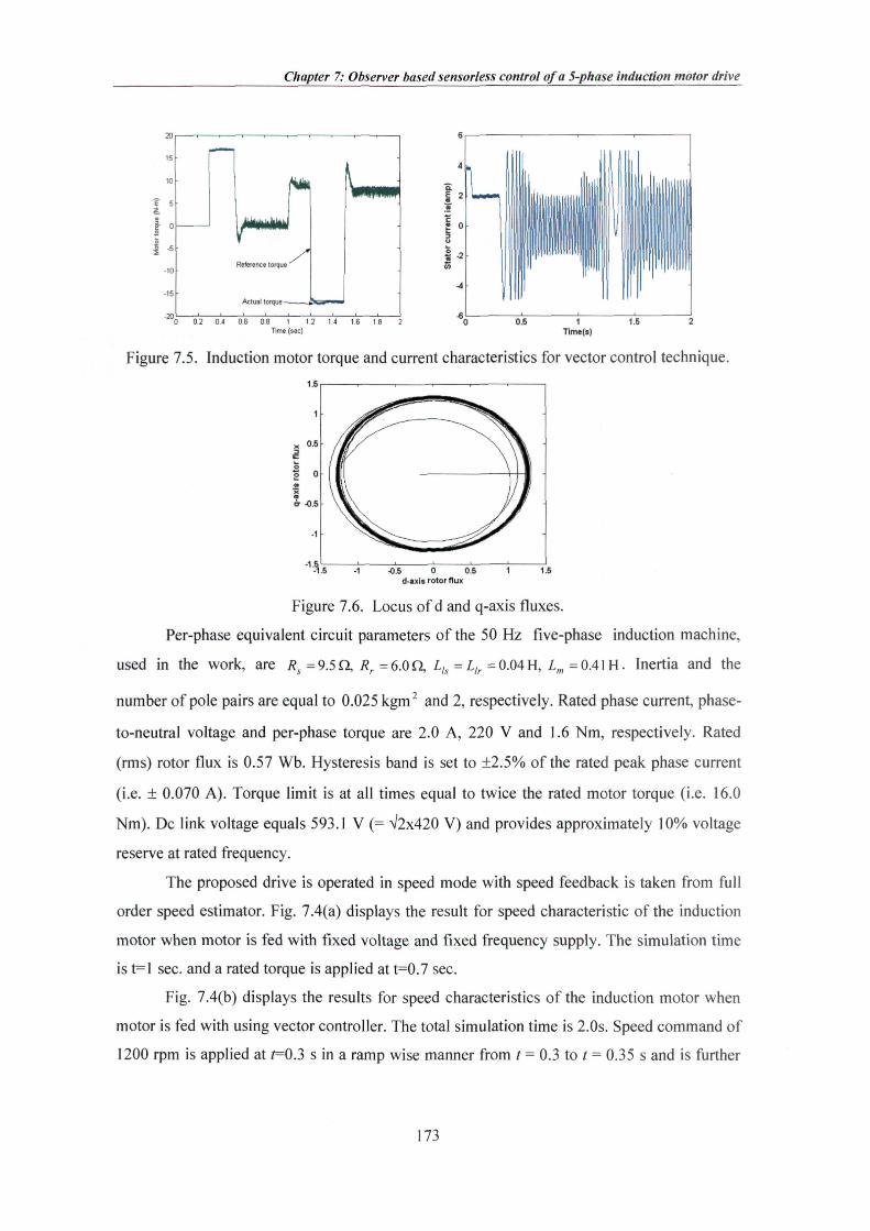
Figure 7.5. Induction motor torque and current characteristics for vector control teclinique.

4 5 0 OS d-axis rotor flux

Figure 7.6. Locus of d and q-axis fluxes.

Per-phase equivalent circuit parameters of the 50 Hz five-phase induction machine,

used in the work, are 7?,-9.5Q,/?^ =6.0Q, I,, =£,, =0.04H, Z,„ =0.41 H. Inertia and the

number of pole pairs are equal to 0.025 kgm^ and 2, respectively. Rated phase current, phase-

to-neutral voltage and per-phase torque are 2.0 A, 220 V and 1.6 Nm, respectively. Rated

(rms) rotor flux is 0.57 Wb. Hysteresis band is set to ±2.5% of the rated peak phase current

(i.e. ± 0.070 A). Torque limit is at all times equal to twice the rated motor torque (i.e. 16.0

Nm). Dc link voltage equals 593.1 V (= ^2x420 V) and provides approximately 10% voltage

reserve at rated frequency.

The proposed drive is operated in speed mode with speed feedback is taken from full

order speed estimator. Fig. 7.4(a) displays the result for speed characteristic of the induction

motor when motor is fed with fixed voltage and fixed frequency supply. The simulation time

is t=l sec. and a rated torque is applied at t=0.7 sec.

Fig. 7.4(b) displays the results for speed characteristics of the induction motor when

motor is fed with using vector controller. The total simulation time is 2.0s. Speed command of

1200 rpm is applied at /=0.3 s in a ramp wise manner from / = 0.3 to / = 0.35 s and is further

173


kept unchanged. Operation takes place under no-load conditions. Disturbance rejection

properties of the drive are investigated next. A load torque equal to the motor rated torque is

applied in a step-wise manner at r = 1 s. Finally, reversing transient is examined as well. The

command for speed reversal is given at / = 1.2 s. The torque and current responses are

obtained for these periods and are shown in Fig. 7.5. It is concluded from the responses that

the actual speed and torque closely follows the reference. Fig. 7.6 displays the results for the

locus of rotor fluxes.

Fig. 7.4(a) and Fig. 7.4(b) shows the five-phase induction motor speed characteristics

for fixed voltage and fixed frequency supply fed and using vector control technique. These

characteristics show production of small ripples in transient as well as in steady-state period

and are better than the characteristics obtained with open-loop speed estimator. In vector

controlled technique, low amplitude ripples are produced in the torque response shown in Fig.

7.5 which is acceptable for sensorless vector controlled induction motor for high performance

drive.

7.3 Kalman filter observer In 1960, R.E. Kalman published his famous paper describing a recursive solution to

the discrete-data linear filtering problem. Since that time, due in large part to advances in

digital computing; the Kalman filter has been the subject of extensive research and

application, particularly in the area of autonomous or assisted navigation.

The Kalman filter is a recursive estimator. This means that only the estimated state

from the previous time step and the current measurement are needed to compute the estimate

for the current state. In contrast to batch estimation techniques, no history of observations

and/or estimates is required. It is unusual in being purely a time domain filter; most filters (for

example, a low-pass filter) are formulated in the frequency domain and then transfoimed back

to the time domain for implementation.

The Kalman filter has two distinct phases: Predict and Update. The predict phase uses

the state estimate from the previous time step to produce an estimate of the state at the current

time step. In the update phase, measurement information at the current time step is used to

refine this prediction to arrive at a new, (hopefully) more accurate state estimate, again for the

current time step.

Kalman filtering is a relatively recent (1960) development in filtering, although it has

its roots as far back as Gauss (1795). Kalman filtering has been applied in areas as diverse as

174


aerospace, marine navigation, nuclear power plant instrumentation, demographic modeling,

manufacturing, and many others.

Some recent studies seeking an observer-based solution to the problem of parameter

variations could be listed as follows; in, a sliding mode based observer is designed for the

estimation of the load torque and rotor flux components by measuring the rotor velocity; with

the nonlinear observer in, the stator fluxes and rotor speed are estimated, while in the

extended Luenberger observer (ELO) in, the rotor fluxes and rotor velocity are estimated, as

well as the step-type load torque. In the literature, a popular method for the state and

parameter estimation of IMs is the extended Kalman filter (EKF). Model uncertainties and

nonlinearities inherent to IMs are well-suited for the stochastic nature of EKFs.

With this method, it is possible to make the on-line estimation of states while

performing the simultaneous identification of parameters in a relatively short time interval,

also taking system/process and measurement errors (noises) directly into account. This is the

reason why EKF has found a wide application range in the sensorless control of IMs, in spite

of its computational complexity. Among recent studies using EKF estimation for IMs, and

estimate the flux and velocity, while uses an adaptive flux-observer in combination with a

second order Kalman filter for the same purpose. None of these studies estimate the load and

rotor resistance, resulting in a performance that is sensitive to the variation of these

parameters. The velocity sensorless study utilizing a velocity sensor and a recursive least-

square algorithm in addition to the EKF, both provide robustness against load, but are

sensitive to variations in the rotor resistance. The velocity is estimated as a constant

parameter, which gives rise to a significant estimation error in the velocity during the

transient state, especially under instantaneous load variations, although the performance is

improved in the steady state. However, the estimation of rotor resistance is performed by the

injection of low amplitude, high frequency signals to the flux reference of direct vector

control system. This has caused fluctuations in the motor flux, torque and speed.

7.3.1 Development of an EKF Algorithm In recent years, the Kalman filter algorithm has been used for the parameter estimation

of an induction motor, or for the speed estimation of a synchronous and an induction motor.

In the speed estimation of an inducfion motor using an extended Kalman filter algorithm, not

only the angular speed of rotor, but also the angular frequency of rotor flux and the angle of

rotor flux have to be augmented in the extended Kalman filter, because the state variables are

175


only the stator currents and magnetizing current. In that case, the complete decoupling of d-q

component fluxes is assumed. Also, the magnetizing current is assumed to be constant.

In the dynamic model of an induction motor, if the dimension of the state vector is

increased by adding an angular speed of rotor, then the state model becomes nonlinear.

Therefore, the extended Kalman filter has to be used to estimate the parameter. In this case,

the angular speed of the rotor is considered as a state and a parameter. The extended Kalman

filter algorithm should be calculated by using a microprocessor, and the system is to be

expressed in a discrete-state model.

An EKF algorithm is developed for the estimation of the states in the extended IM

model given in (7.12) and (7.13), to be used in the sensorless vector control of the IM. The

Kalman filter is a well-known recursive algorithm that takes the stochastic state space model

of the system into account, together with measured outputs, to achieve the optimal estimation

of states in multi-input, multi-output systems. The system and measurement noises are

considered to be in the form of white noise. The optimality of the state estimation is achieved

with the minimization of the covariance of the estimation error. For nonlinear problems, the

KF is not strictly applicable since linearity plays an important role in its derivation and

performance as an optimal filter. The EKF attempts to overcome this difficulty by using a

linearized approximation where the linearization is performed about the current state estimate.

This process requires the discretization of (7.12) and (7.13);

Kalman filter is a unique observer which offers best possible filtering of the noise in

measurement and of the system if the noise covariances are known. If rotor speed considered

as an extended state and is incorporated in the dynamic model of an induction machine then

the extended Kalman filter can be used to relinearize the nonlinear state model for each new

value of estimate. As a result, the extended Kalman filter is measured to be the best solution

for the speed estimation of an induction machine. The extended Kalman filter has been

applied to the vector control system and for a direct control system or a constant Volt per

Hertz. Few publications have been reported for the choice of the covariance matrices of the

Kalman speed estimator. In this paper, the Kalman speed estimator for a vector controlled

five-phase induction motor drive system is studied.

7.3.2 Kalman Filters

Kalman filter takes care of the effects of the disturbance noise of a control system and

the errors in the parameters of the system are considered as noise. The Kalman filter can be

expressed as a state model:

176


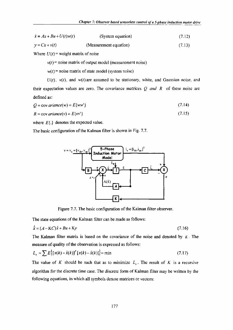
x = Ax + Bu + U(t)wit) (System equation) (7.12)

y = Cx + v(/) (Measurement equation) (7.13)

Where f/(/)= weight matrix of noise

v{t)= noise matrix of output model (measurement noise)

^ 0 = noise matrix of state model (system noise)

(/(/), v(/), and >v(/)are assumed to be stationary, white, and Gaussian noise, and

their expectation values are zero. The covariance matrices Q and R of these noise are

defined as:

Q = co\ ariance(w) = E{ww'} (7.14)

R = co\ariance{v)-E{w'} (7.15)

where E{.} denotes the expected value.

The basic configuration of the Kalman filter is shown in Fig. 7.7.

V = Vs=[Vds.VqjJ 5-Phase Induction Motor

Model

's - [ 'ds ' iqs]

K'e "+?+

Xol

A(x) {A>

•*[iH^-t©

•H^

Figure 7.7. The basic configuration of the Kalman filter observer.

The state equations of the Kalman filter can be made as follows:

x = (A-KC)x + Bu + Ky (7.16)

The Kalman filter matrix is based on the covariance of the noise and denoted by K. The

measure of quality of the observation is expressed as follows:

I , ^^E{[xik)-x(k)Y[xik)-x(k)]}=mm (7.17)

The value of K should be such that as to minimize L^. The result of K is a recursive

algorithm for the discrete time case. The discrete form of Kalman filter may be written by the

following equations, in which all symbols denote matrices or vectors:

177


(i) System state estimation:

x{k +1) = x{k) + Y.{k)(y{k) - y{k)) (7.18)

(ii) Renew of the error covariance matrix:

P{k +1) = P{k) - K{k)h^ (k + l)Pik) (7.19)

(iii)Calculation of Kaiman filter gain matrix:

Kik + l) = F'ik + \)h^(k + \)[h{k + 1)P* (k + l)h^ (/t +1) + R]'' (7.20)

(iv) Prediction of state matrix:

/ (^ + l) = £ ( A x + 5,v)|,.,,,,„ (7.21)

(v) Estimation of error covariance matrix:

P'(k + l) = f(k + \)hk)f ( +1) + 0 (7.22)

Discretization of (7.25) and (7.26) yields:

x{k + \) = A, {k)x{k) + B, {k)u{k) (7.23)

yik) = CAk)x{k) (7.24)

where K{k)\s the feedback matrix of the Kaiman filter. K{k) gain matrix calculates

how the state vector of the Kaiman filter is updated when the output of the model is compared

with the actual output of the system. The Kaiman filter algorithm can also be used for

nonlinear systems (e.g. induction motor). However, the optimal performance may not be

obtained and it is impractical to verify the convergence of the model. To realize the recursive

algorithm of the extended Kaiman filter, a state model of the induction motor is required.

After knowing the matrices^^, Bj, and C^, the matrices x(k) (state prediction) and y(k)

(output prediction) can be calculated.

7.3.3 Design of extended Kaiman filter for a five-phase induction motor drive When rotor speed is considered as a state variable in the induction motor model, then

an extended induction motor model is obtained and the rotor speed is considered as an

extended state. The discrete induction motor model defined in equations (7.23) and (7.24) can

be implemented in the extended Kaiman filter algorithm.

If the system matrix, the input and output matrices of the discrete system are denoted

hyAj, Bj, and Cj, while the state and the output of the discrete system are denoted by

x(^)and >'(A:),then

178


A,-

\-TIT' 0

0 i - r / r ;

TLJT^ 0

0 TLjr

0 0

TLJiL^LX) coJLJiL^L^) 0

-coJLJ{L,L^) TLJiL^LX) 0

\-TIT^ -Tco^ 0

Tco^ \-TIT^ 0

0 0 1

B,=

TIL,

0

0

0

0

0

TIL,

0

0

0

c,= 1 0 0 0 0

0 1 0 0 0

x{k) = [/,, {k)i^, {k)yy,, (k),^^, {k)co, {k)f

u{k) = [u^{k)u^,{k)f

where I , = oi , = (1 - - - ^ ) Z , , 7; * = •

(7.25)

(7.26)

(7.27)

and T is the sampling time. 4 4 ' - ^ R,+R,(LJLy

The essential matrices and vectors for the recursive algorithm of the extended Kalman

filter can be calculated, with the discrete system model. With the help of Matlab/Simulink

program, speed estimation algorithm of the extended Kalman filter can be simulated, as

shown in Fig.7.8. The execution of the S-flinction block is based on an M-file written as

MATLAB code.

From3

Kalmjn M File

S-Function

Ids

-KZD

Iqs

Fds

•XZD Fqs -KID

Speed

Figure 7.8. Simulink based extended Kalman filter speed estimator.

179


7.3.4 Sensorless operation of a five-phase induction motor drives using EKF algorithm The developed model of a five-phase induction motor indicates that an observer

(Kalman Filter) used for three-phase machines can be easily extended to multi-phase

machines. For multi-phase machines observer-based speed estimator requires only d and q

components of stator voltages and currents. From the model of a five-phase induction

machine, it is shown that the stator and rotor d and q axis flux linkages are function of

magnetizing inductance Lm and stator and rotor d and q axis currents, where as the x and y

axis flux linkages are function of only their respective currents. Therefore in speed estimation

for multi-phase machine the x and y components of voltages and currents are not required.

The speed can be estimated using only c? and q components of stator voltages and currents.

The proposed extended Kalman filter-based vector controlled five-phase induction motor

drive structure with current control in the stationary reference frame is shown in Fig. 7.9.

Diode Bridge

AC Supely ^ Rectifier

J* PWM VSI

(O I, 2

Hysteresis Current Controller

*ds''q

Kalman Filter based speed

controller

6

CO :ontroller ^ " ^ ^ y T T

-i H L H ; O^

l - "h;

Induction Motor Eddy current loading

Figure 7.9. A vector controlled five-phase induction motor with extended Kalman filter speed estimation algorithm. ,

7.3.5 Simulation results

0 4 0 6 Tim« (s«c)

1600

1400

12CB

•§• 1000

S 800

I 600

I 400

200

0

200

•

/

,

1 ^Actual speed

/ ^^eference speed

Speed errof

•

/ Loading

1

•

0 01 02 03 04 05 06 07 08 09 1 Time (sec)

Figure 7.10. Five-phase induction motor torque and speed characteristics for fixed voltage and fixed frequency fed supply {g^ = q^=\Q-6, g2 = (?2=le-2).

180


•

1

speed \

Reference speed - ^

f Speed error

\ •

\

Time (sec) 0 02 04 06 08 1 12 14 16 18 2

Time (sec)

Figure 7.11. Five-phase induction motor torque and speed characteristics for vector control (gi='7i=le-6, g2 = ^2='e-2).

-06 0 0 5 d-axis folor fluK (wb)

Figure 7.12. Locus of rotor d- and q-axis fluxes. The proposed drive is operated in speed mode with speed feedback is taken from

Kalman filter speed estimator. Fig. 7.10 displays the results for torque and speed

characteristics of the induction motor when motor is fed with fixed voltage and fixed

frequency supply. The simulation time is t=l sec. and a rated torque is applied at t=0.7 sec.

For vector control, the total simulation time is t=2 sec. Speed command of 1200 rpm is

functional at /=0.3 sec in a ramp wise mode from / = 0.3 to / = 0.35 sec and is further kept

unaffected. Operation takes place under no-load and load conditions. Interruption dismissal

properties of the drive are investigated next. A load torque equal to the motor rated torque is

functional in a step-wise mode at / = 1 sec. In the last, reversing transient is examined. The

command for speed reversal is given at r = 1.2 sec. The results, obtained for these periods, are

shown in Fig. 7.11. It is concluded from the results that, the actual speed and torque closely

follow the reference. Fig. 7.12 displays the locus of rotor fluxes.

The five-phase induction motor torque and speed characteristics for fixed voltage and

fixed frequency fed supply (g|=^|=le-6, g2^72^'s-2) is shown in Fig. 7.10. These

characteristics show production of very small ripples in transient as well as in steady-state

181


period and are better than the characteristics obtained with Luenberger observer based speed

estimator. In vector controlled technique, low amplitude ripples are produced in the torque

and speed responses shown in Fig. 7.11, which is acceptable for sensorless vector controlled

induction motor for high performance drive. The responses obtained with Kalman filter based

speed estimator are much superior to open-loop estimator responses because this estimator is

free from integrators and differentiators.

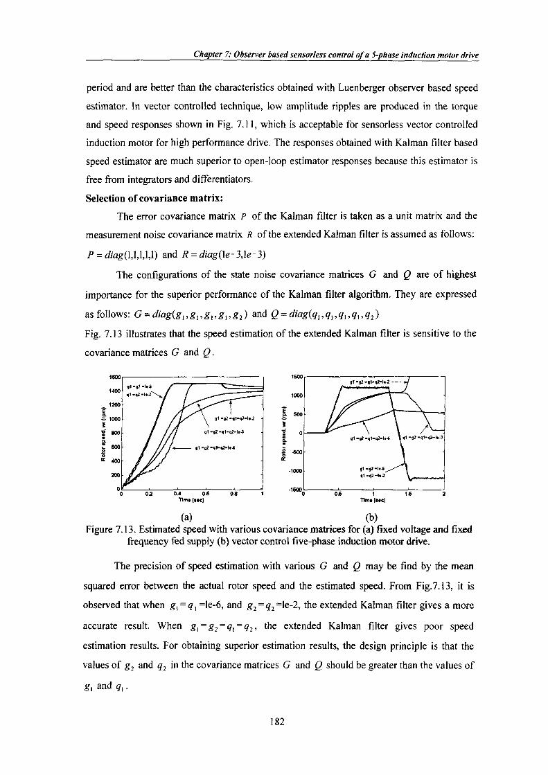
Selection of covariance matrix:

The error covariance matrix P of the Kalman filter is taken as a unit matrix and the

measurement noise covariance matrix R of the extended Kalman filter is assumed as follows;

P = /ag(l,l,l,l,l) and R = diag{\e-3,\e-3)

The configurations of the state noise covariance matrices G and Q are of highest

importance for the superior performance of the Kalman filter algorithm. TTiey are expressed

as follows: G = diagig^,gi,gi,gi,g2) andQ = diag(qi,?,,^,,9,,^j)

Fig. 7.13 illustrates that the speed estimation of the extended Kalman filter is sensitive to the

covariance matrices G and Q.

g1 -g2 -ql-a2-l« J

g1 -92 -ql-q2-le-3

g1 "92 -<|1-92-t**

0.4 0.6 Tltni (MC)

1000

L SCO

0

«00

•1000

-1600.

j 1 -j|2 -q1«q2-U.2 f^

| 1 - j J - 1 . 4

4l -<|2 -l<.2

0.6 1 T lmt ( t tc )

1.6

(a) (b) Figure 7.13. Estimated speed with various covariance matrices for (a) fixed voltage and fixed

frequency fed supply (b) vector control five-phase induction motor drive.

The precision of speed estimation with various G and Q may be find by the mean

squared error between the actual rotor speed and the estimated speed. From Fig.7.13, it is

observed that when g, = ^, =le-6, and g2 = 92^1e-2, the extended Kalman filter gives a more

accurate result. When g\-g2~<i\~92^ the extended Kalman filter gives poor speed

estimation results. For obtaining superior estimation results, the design principle is that the

values of g^ and q^ in the covariance matrices G and Q should be greater than the values of

g, and q, .

182


lA Comparison between adaptive flux observer and extended Kalman filter-based algorithms for sensorless vector controlled five-phase induction motor drive

This section presents a comparison between the performances of an adaptive flux

observer and those of extended Kalman filter-based algorithms, used to estimate the rotor

speed in a vector-controlled five-phase induction motor drive. The estimate is obtained by

measuring stator voltages and stator currents in both schemes. Performance of vector

controlled drive system is investigated for acceleration, loading and reversing transients.

Particularly, the influence of random noise, in stator voltages and currents

measurements, on the estimation accuracy has been tested for both the algorithms. Many

computer simulations carried out in Matlab/Simulink environment have proved the

performances of both the algorithms.

7.4.1 Simulation results and discussion i

/

Speed eirM

i

1600

1400

1200

• 1000

BOO

600

200 • /

/

^V, /

Loading

" • ^ B f e m

04 06 Time (sec)

01 02 03 04 05 06 07 08 09 Trme (sec)

(a) (b) Figure 7.14. Fixed voltage and fixed frequency supply fed five-phase induction motor drive

speed characteristics for (a) an adaptive fiux observer and (b) extended Kalman filter.

M

1

f i 08

o 06 o

04

U

-

1 f ' 1 Commanded flux

^ ^ . —/ ^'^1^

Acliidl fitix .

•

•

•

•

12

1

1 06

I 06

r\ Commanded llui

OS 1 Time (see)

0 02 04 06 08 I 12 14 1 6 IE Time (sec)

(a) (b) Figure 7.15. Vector controlled five-phase induction motor drive rotor flux characteristics for

(a) adaptive flux observer and (b) extended Kalman filter.

183


1600

1000

I -sooh a.

-1600 05 1 15

Time (sec)

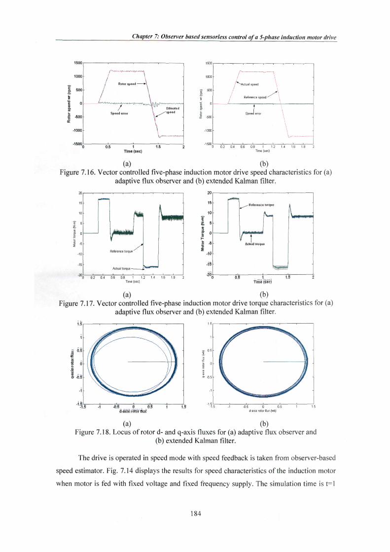
(a) (b) Figure 7.16. Vector controlled five-phase induction motor drive speed characteristics for (a)

adaptive flux observer and (b) extended Kalman filter.

B

I Reference torque

Actual torque -

02 04 06 08 1 12 H 16 18 2 Time (sec)

(a) (b) Figure 7.17. Vector controlled five-phase induction motor drive torque characteristics for (a)

adaptive flux observer and (b) extended Kalman filter.

•OS 0 05 d-axis rotor fluV

-05 0 05 d-8X(S fOtorHdK (vib)

(a) (b) Figure 7.18. Locus of rotor d- and q-axis fluxes for (a) adaptive flux observer and

(b) extended Kalman filter.

The drive is operated in speed mode with speed feedback is taken from observer-based

speed estimator. Fig. 7.14 displays the results for speed characteristics of the induction motor

when motor is fed with fixed voltage and fixed frequency supply. The simulation time is t=l

184


s. and a rated torque is applied at t=0.7 s. For vector control, the total simulation time is t=2 s.

Speed command of 1200 rpm is applied at /=0.3 s in a ramp wise manner from / = 0.3 to / =

0.35 s and is ftjrther kept unchanged. Operation takes place under no-load conditions.

Disturbance rejection properties of the drive are investigated next. A load torque equal to the

motor rated torque is applied in a step-wise manner at / = 1 s. Finally, reversing transient is

examined as well. The command for speed reversal is given at / = 1.2 s. The responses,

obtained for these periods, are shown in Fig. 7.15, 7.16 and 7.17. It is concluded from the

responses that the actual speed and torque closely follows the reference. Fig. 7.18 displays the

results for the locus of rotor fluxes.

When drive is fixed voltage and fixed frequency fed then maximum speed fluctuation in

adaptive flux observer and extended kalman filter are 20 rpm and 10 rpm respectively. This

speed error is in acceleration period only and in steady-state period error is approximately

zero. When drive is vector controlled then maximum fluctuation in rotor flux are 0.1 wb and

0.05 wb, called as loss of vector control and the speed errors are 50 rpm and 5 rpm and the

torque fluctuations are 2.5 N-m and 1.0 N-m respectively. In adaptive flux observer, the

torque response is of oscillatory nature, this is due to the application of PID controller in the

observer. This oscillatory response is absent in extended Kalman filter because PID is not

used. Therefore Kalman filter shows superior performances with respect to adaptive observer.

7.5 Summary The first part of this chapter deals with fiall order observer-based sensorless vector

control of a five-phase induction machine, utilising an indirect rotor flux oriented controller

and current control in stationary reference frame is at first reviewed and it is shown that the

resulting model is the same as for a three-phase machine rotor flux oriented controller and

current control in the stationary reference frame. Hence the same vector control principles and

speed estimation technique are applicable. Operation in the speed mode is further studied,

utilising the hysteresis current control. The speed feedback signal is the estimated one

obtained from observer -based speed estimator. The attainable performance is examined by

simulation. It is shown that the dynamic behaviour, obtainable with the indirect vector

control, is the same as it would have been had a three-phase machine been used. Rotor flux

and torque control are fully decoupled, enabling the fastest possible accelerations and

decelerations with the given torque limit.

In second part of this chapter, an extended Kalman filter is designed to estimate the

rotor speed of a vector controlled five-phase induction motor drive. Effects of the covariance

185


matrices of the Kalman filter are studied and a suggestion for selecting the covariance

matrices is also given. Simulation results shows that the extended Kalman filter has excellent

noise rejection properties. The attainable performance are examined by simulation and

compared. It is shown that the dynamic behavior, obtainable with the indirect vector control,

is the same as obtained with three-phase machine. Same technique can be extended to multi

phase multi-motor drive system.

This chapter presents a detailed study of a fiill order Luenberger observer and

extended Kalman filter based sensorless control of a five-phase induction motor drive and

then comparison between the performances of an adaptive flux observer and those of an

extended Kalman filter-based algorithm, used to estimate the rotor flux components, and so

the rotor speed. Simulation results have shown the superior performances of Kalman filter

with respect to adaptive observer.

186

chapter 7 observer based sensorless control of...

Documents