chapter 7: modeling radiation and natural convection

Chapter 7: Modeling Radiation and Natural Convection

This tutorial is divided into the following sections:

7.1. Introduction

7.2. Prerequisites

7.3. Problem Description

7.4. Setup and Solution

7.5. Summary

7.6. Further Improvements

7.1. Introduction

In this tutorial, combined radiation and natural convection are solved in a three-dimensional square

box on a mesh consisting of hexahedral elements.

This tutorial demonstrates how to do the following:

• Use the surface-to-surface (S2S) radiation model in ANSYS FLUENT.

• Set the boundary conditions for a heat transfer problem involving natural convection and radiation.

• Calculate a solution using the pressure-based solver.

• Display velocity vectors and contours of wall temperature, surface cluster ID, and radiation heat flux.

7.2. Prerequisites

This tutorial is written with the assumption that you have completed Introduction to Using ANSYS FLUENT:

Fluid Flow and Heat Transfer in a Mixing Elbow (p. 131), and that you are familiar with the ANSYS FLU-

ENT navigation pane and menu structure. Some steps in the setup and solution procedure will not be

shown explicitly.

7.3. Problem Description

The problem to be considered is shown schematically in Figure 7.1 (p. 308). A three-dimensional box

× × has a hot wall of aluminum at 473 K. All other walls are made of an

insulation material and are subject to radiative and convective heat transfer to the surroundings which

are at 293 K. Gravity acts downwards. The medium contained in the box is assumed not to emit, absorb,

or scatter radiation. All walls are gray. The objective is to compute the flow and temperature patterns

in the box, as well as the wall heat flux, using the surface-to-surface (S2S) model available in ANSYS

FLUENT.

The working fluid has a Prandtl number of approximately 0.71, and the Rayleigh number based on �

(0.25) is × �. This means the flow is most likely laminar. The Planck number � ��

� is 0.006,

and measures the relative importance of conduction to radiation.

307Release 14.0 - © SAS IP, Inc. All rights reserved. - Contains proprietary and confidential information

of ANSYS, Inc. and its subsidiaries and affiliates.

Figure 7.1 Schematic of the Problem

7.4. Setup and Solution

The following sections describe the setup and solution steps for this tutorial:

7.4.1. Preparation

7.4.2. Step 1: Mesh

7.4.3. Step 2: General Settings

7.4.4. Step 3: Models

7.4.5. Step 4: Materials

7.4.6. Step 5: Boundary Conditions

7.4.7. Step 6: Solution

7.4.8. Step 7: Postprocessing

7.4.9. Step 8: Compare the Contour Plots after Varying Radiating Surfaces

7.4.10. Step 9: S2S Definition, Solution and Postprocessing with Partial Enclosure

7.4.1. Preparation

1. Extract the file radiation_natural_convection.zip from the ANSYS_Fluid_Dynamics_Tu-torial_Inputs.zip archive which is available from the Customer Portal.

Note

For detailed instructions on how to obtain the ANSYS_Fluid_Dynamics_Tutori-al_Inputs.zip file, please refer to Preparation (p. 3) in Introduction to Using ANSYS

FLUENT in ANSYS Workbench: Fluid Flow and Heat Transfer in a Mixing Elbow (p. 1).

2. Unzip radiation_natural_convection.zip to your working folder.

The mesh file rad.msh.gz can be found in the radiation_natural_convection folder created

after unzipping the file.

Release 14.0 - © SAS IP, Inc. All rights reserved. - Contains proprietary and confidential informationof ANSYS, Inc. and its subsidiaries and affiliates.308


http://www.ansys.com/customerportal/

3. Use FLUENT Launcher to start the 3D version of ANSYS FLUENT.

For more information about FLUENT Launcher, see Starting ANSYS FLUENT Using FLUENT

Launcher in the User’s Guide.

Note

The Display Options are enabled by default. Therefore, after you read the mesh, it will be

displayed in the embedded graphics window.

7.4.2. Step 1: Mesh

1. Read the mesh file rad.msh.gz .

File → Read → Mesh...

As the mesh is read, messages will appear in the console reporting the progress of the reading. The

mesh size will be reported as 64,000 cells.

7.4.3. Step 2: General Settings

General

1. Check the mesh.

General → Check

ANSYS FLUENT will perform various checks on the mesh and report the progress in the console. Make

sure that the reported minimum volume is a positive number.

2. Examine the mesh.



Setup and Solution

Figure 7.2 Graphics Display of Mesh

3. Retain the default solver settings.

General



4. Enable Gravity.

a. Enter -9.81 � �� for Gravitational Acceleration in the Y direction.

7.4.4. Step 3: Models

Models

1. Enable the energy equation.

Models → Energy → Edit...

2. Enable the Surface to Surface (S2S) radiation model.

Models → Radiation → Edit...



Setup and Solution

a. Select Surface to Surface (S2S) in the Model list.

The Radiation Model dialog box will expand to show additional inputs for the S2S model.

The surface-to-surface (S2S) radiation model can be used to account for the radiation exchange

in an enclosure of gray-diffuse surfaces. The energy exchange between two surfaces depends in

part on their size, separation distance, and orientation. These parameters are accounted for by

a geometric function called a “view factor”.

The S2S model assumes that all surfaces are gray and diffuse. Thus according to the gray-body

model, if a certain amount of radiation is incident on a surface, then a fraction is reflected, a

fraction is absorbed, and a fraction is transmitted. The main assumption of the S2S model is that

any absorption, emission, or scattering of radiation by the medium can be ignored. Therefore

only “surface-to-surface” radiation is considered for analysis.

For most applications the surfaces in question are opaque to thermal radiation (in the infrared

spectrum), so the surfaces can be considered opaque. For gray, diffuse, and opaque surfaces it is

valid to assume that the emissivity is equal to the absorptivity and that reflectivity is equal to 1

minus the emissivity.

When the S2S model is used, you also have the option to define a “partial enclosure” which allows

you to disable the view factor calculation for walls with negligible emission/absorption or walls

that have uniform temperature. The main advantage of this option is to speed up the view factor

calculation and the radiosity calculation.

b. Click the Settings... button to open the View Factors and Clustering dialog box.

You will define the view factor and cluster parameters.



i. Retain the value of 1 for Faces per Surface Cluster for Flow Boundary Zones in the

Manual group box.

ii. Click Apply to All Walls.

The S2S radiation model is computationally very expensive when there are a large number

of radiating surfaces. The number of radiating surfaces is reduced by clustering surfaces into

surface “clusters”. The surface clusters are made by starting from a face and adding its

neighbors and their neighbors until a specified number of faces per surface cluster is collected.

For a small problem, the default value of 1 for Faces per Surface Cluster for Flow

Boundary Zones is acceptable. For a large problem you can increase this number to reduce

the memory requirement for the view factor file that is saved in a later step. This may also

lead to some reduction in the computational expense. However, this is at the cost of some

accuracy. This tutorial illustrates the influence of clusters.

iii. Ensure Ray Tracing is selected from the Method list in the View Factors group box.

iv. Click OK to close the View Factors and Clustering dialog box.

c. Click Compute/Write/Read... in the View Factors and Clustering group box to open the SelectFile dialog box and to compute the view factors.

The file created in this step will store the cluster and view factor parameters.



Setup and Solution

i. Enter rad_1.s2s.gz as the file name for S2S File.

ii. Click OK in the Select File dialog box.

Note

The size of the view factor file can be very large if not compressed. It is highly

recommended to compress the view factor file by providing .gz or .Z exten-

sion after the name (i.e. rad_1.gz or rad_1.Z ). For small files, you can

provide the .s2s extension after the name.

ANSYS FLUENT will print an informational message describing the progress of the view factor

calculation in the console.

d. Click OK to close the Radiation Model dialog box.

7.4.5. Step 4: Materials

Materials

1. Set the properties for air.

Materials → air → Create/Edit...

a. Select incompressible-ideal-gas from the Density drop-down list.

b. Enter 1021 J/kg-K for Cp (Specific Heat).

c. Enter 0.0371 W/m-K for Thermal Conductivity.

d. Enter 2.485e-05 kg/m-s for Viscosity.



e. Retain the default value of 28.966 kg/kmol for Molecular Weight.

f. Click Change/Create and close the Create/Edit Materials dialog box.

2. Define the new material, insulation.

Materials → Solid → Create/Edit...

a. Enter insulation for Name and delete the entry in the Chemical Formula field.

b. Enter 50 �� for Density.

c. Enter 800 J/kg-K for Cp (Specific Heat).

d. Enter 0.09 W/m-K for Thermal Conductivity.

e. Click Change/Create.

A Question dialog box will open, asking if you want to overwrite aluminum.

f. Click No in the Question dialog box to retain aluminum and add the new material (insulation)

to the materials list.



Setup and Solution

The Create/Edit Materials dialog box will be updated to show the new material, insulation, in

the FLUENT Solid Materials drop-down list.

g. Close the Create/Edit Materials dialog box.

7.4.6. Step 5: Boundary Conditions

Boundary Conditions

1. Set the boundary conditions for the front wall (w-high-x).

Boundary Conditions → w-high-x → Edit...



a. Click the Thermal tab and select Mixed in the Thermal Conditions group box.

b. Select insulation from the Material Name drop-down list.

c. Enter 5 −� � ��

for Heat Transfer Coefficient.

d. Enter 293.15 K for Free Stream Temperature.

e. Enter 0.75 for External Emissivity.

f. Enter 293.15 K for External Radiation Temperature.

g. Enter 0.95 for Internal Emissivity.

h. Enter 0.05 m for Wall Thickness.

i. Click OK to close the Wall dialog box.

2. Copy boundary conditions to define the side walls w-high-z and w-low-z.

Boundary Conditions → Copy...



Setup and Solution

a. Select w-high-x from the From Boundary Zone selection list.

b. Select w-high-z and w-low-z from the To Boundary Zones selection list.

c. Click Copy.

A Warning dialog box will open, asking if you want to copy the boundary conditions of w-high-

x to w-high-z and w-low-z.

d. Click OK in the Warning dialog box.

e. Close the Copy Conditions dialog box.

3. Set the boundary conditions for the heated wall (w-low-x).

Boundary Conditions → w-low-x → Edit...



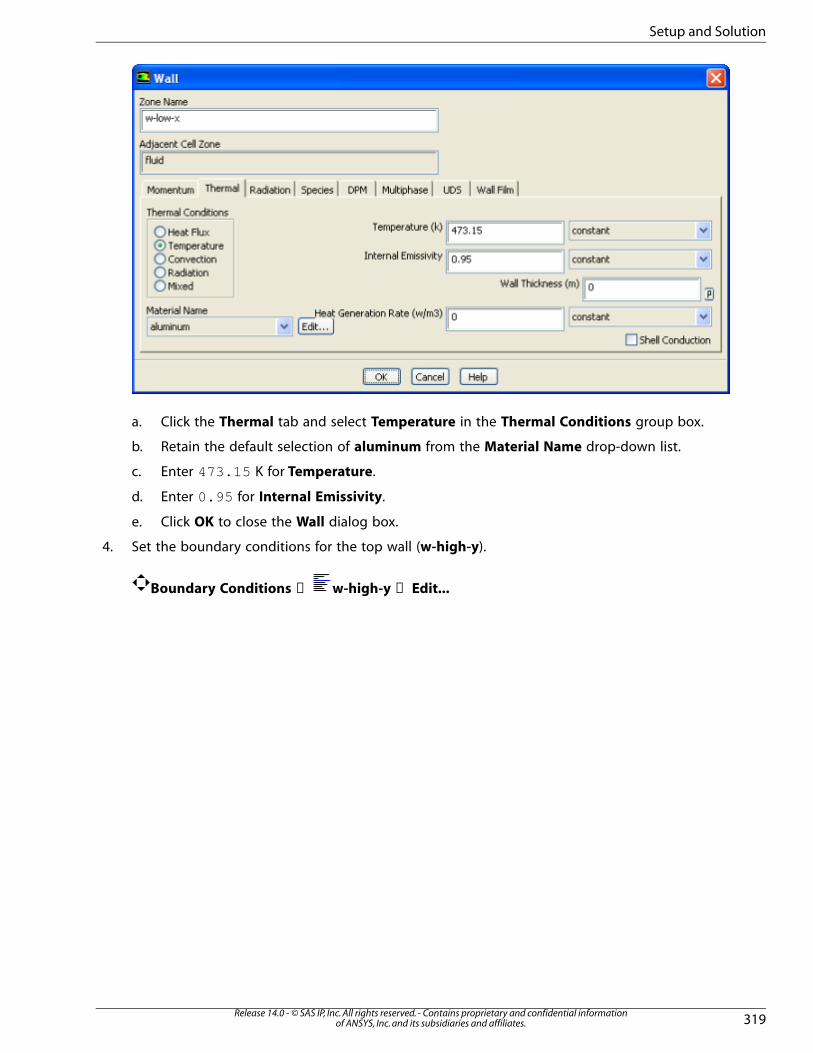
a. Click the Thermal tab and select Temperature in the Thermal Conditions group box.

b. Retain the default selection of aluminum from the Material Name drop-down list.

c. Enter 473.15 K for Temperature.

d. Enter 0.95 for Internal Emissivity.

e. Click OK to close the Wall dialog box.

4. Set the boundary conditions for the top wall (w-high-y).

Boundary Conditions → w-high-y → Edit...



Setup and Solution

a. Click the Thermal tab and select Mixed in the Thermal Conditions group box.

b. Select insulation from the Material Name drop-down list.

c. Enter 3 −� � ��

for Heat Transfer Coefficient.

d. Enter 293.15 K for Free Stream Temperature.

Enter 0.75 for External Emissivity.

e. Enter 293.15 K for External Radiation Temperature.

f. Enter 0.95 for Internal Emissivity.

g. Enter 0.05 m for Wall Thickness.

h. Click OK to close the Wall dialog box.

5. Copy boundary conditions to define the bottom wall (w-low-y).

Boundary Conditions → Copy...



a. Select w-high-y from the From Boundary Zone selection list.

b. Select w-low-y from the To Boundary Zones selection list.

c. Click Copy.

A Warning dialog box will open, asking if you want to copy the boundary conditions of w-high-

y to w-low-y.

d. Click OK in the Warning dialog box.

e. Close the Copy Conditions dialog box.

7.4.7. Step 6: Solution

1. Set the solution parameters.

Solution Methods



Setup and Solution

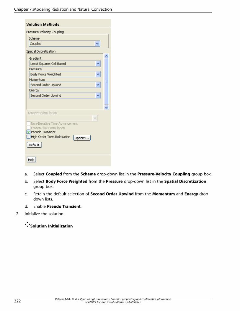
a. Select Coupled from the Scheme drop-down list in the Pressure-Velocity Coupling group box.

b. Select Body Force Weighted from the Pressure drop-down list in the Spatial Discretizationgroup box.

c. Retain the default selection of Second Order Upwind from the Momentum and Energy drop-

down lists.

d. Enable Pseudo Transient.

2. Initialize the solution.

Solution Initialization



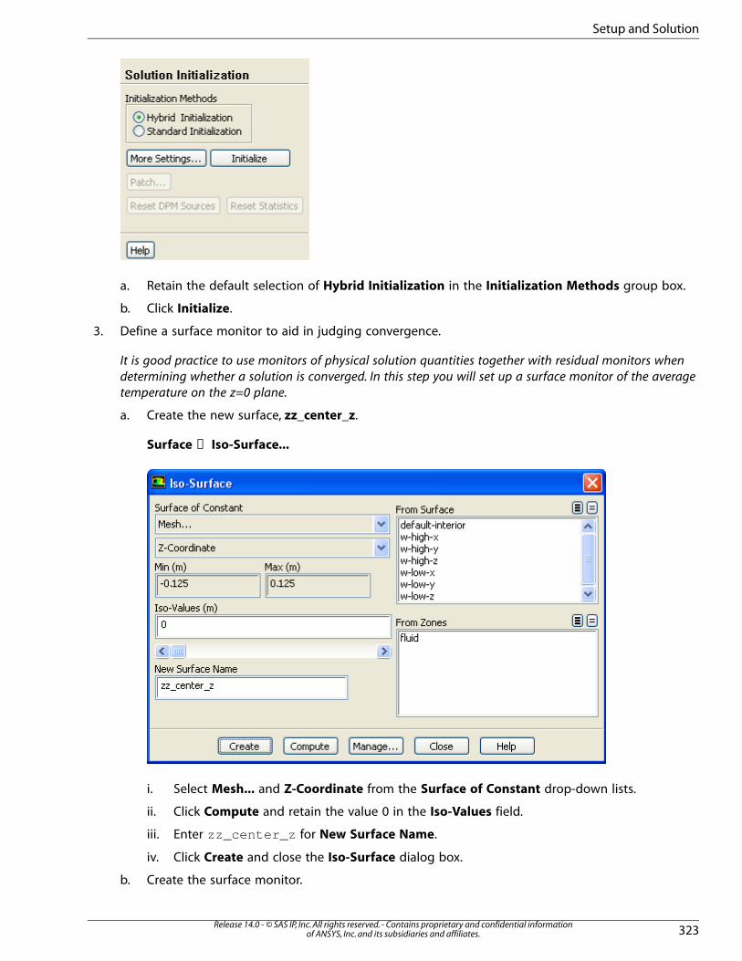
a. Retain the default selection of Hybrid Initialization in the Initialization Methods group box.

b. Click Initialize.

3. Define a surface monitor to aid in judging convergence.

It is good practice to use monitors of physical solution quantities together with residual monitors when

determining whether a solution is converged. In this step you will set up a surface monitor of the average

temperature on the z=0 plane.

a. Create the new surface, zz_center_z.

Surface → Iso-Surface...

i. Select Mesh... and Z-Coordinate from the Surface of Constant drop-down lists.

ii. Click Compute and retain the value 0 in the Iso-Values field.

iii. Enter zz_center_z for New Surface Name.

iv. Click Create and close the Iso-Surface dialog box.

b. Create the surface monitor.



Setup and Solution

Monitors (Surface Monitors) → Create...

i. Retain the default entry of surf-mon-1 for the Name of the surface monitor.

ii. Enable the Plot option.

Note

Unlike residual values, data from other monitors is not saved as part of the

solution set when the ANSYS FLUENT data file is saved. If you want to access

the surface monitor data in future ANSYS FLUENT sessions, you can enable

the Write option and specify a file name for the monitor output.

iii. Select Area-Weighted Average from the Report Type drop-down list.

iv. Select Temperature... and Static Temperature from the Field Variable drop-down lists.

v. Select zz_center_z from the Surfaces selection list.

vi. Click OK to save the surface monitor settings and close the Surface Monitor dialog box.

4. Save the case file (rad_a_1.cas.gz )

File → Write → Case...

5. Start the calculation by requesting 300 iterations (Figure 7.3 (p. 326)).

Run Calculation



a. Select User Specified in the Time Step Method group box. Retain the default value of 1 for

Pseudo Time Step (s).

b. Enter 300 for Number of Iterations.

c. Click Calculate.



Setup and Solution

Figure 7.3 Scaled Residuals

The residual values indicate that the solution has apparently converged. To confirm, you will also inspect

the results for the surface monitor you set up previously.



Figure 7.4 Temperature Surface Monitor

The surface monitor history shows that the Average Temperature on zz_center_z has stabilized con-

firming that the solution has converged as indicated by the residual values.

7.4.8. Step 7: Postprocessing

1. Create a new surface, zz_x_side, which will be used later to plot wall temperature.

Surface → Line/Rake...



Setup and Solution

a. Enter (-0.125, 0, 0.125) for (x0, y0, z0) respectively.

b. Enter (0.125, 0, 0.125) for (x1, y1, z1) respectively.

c. Enter zz_x_side for New Surface Name.

d. Click Create and close the Line/Rake Surface dialog box.

2. Display contours of static temperature.

Graphics and Animations → Contours → Set Up...



a. Enable Filled in the Options group box.

b. Select Temperature... and Static Temperature from the Contours of drop-down lists.

c. Select zz_center_z from the Surfaces selection list.

d. Enable Draw Mesh in the Options group box to open the Mesh Display dialog box.

i. Select Outline in the Edge Type list.

ii. Click Display and close the Mesh Display dialog box.

e. Disable Auto Range.

f. Enter 421 K for Min and 473.15 K for Max.

g. Click Display and rotate the view as shown in Figure 7.5 (p. 330).

h. Close the Contours dialog box.



Setup and Solution

Figure 7.5 Contours of Static Temperature

A regular check for most buoyant cases is to look for evidence of stratification in the temperature field.

This is observed as nearly horizontal bands of similar temperature. These may be broken or disturbed

by buoyant plumes. For this case you can expect reasonable stratification with some disturbance at

the vertical walls where the air is driven around. Inspection of the temperature contours in Figure

7.5 (p. 330) reveals that the solution appears as expected.

3. Display contours of wall temperature (outer surface).




a. Make sure that Filled is enabled in the Options group box.

b. Disable Node Values.

c. Select Temperature... and Wall Temperature (Outer Surface) from the Contours of drop-down

lists.

Note

In the context of the Wall Temperature field variables, Outer Surface refers to

whichever surface of the wall is in contact with the fluid domain. This may or may

not correspond to an “outer” wall of the problem geometry.

d. Select all surfaces except default-interior and zz_x_side.

e. Disable Auto Range and Draw Mesh.

f. Enter 413 K for Min and 473.15 K for Max.

g. Click Display and rotate the view as shown in Figure 7.6 (p. 332).



Setup and Solution

Figure 7.6 Contours of Wall Temperature

4. Display contours of radiation heat flux.





b. Disable both Node Values and Draw Mesh in the Options group box.

c. Select Wall Fluxes... and Radiation Heat Flux from the Contours of drop-down list.


e. Click Display and rotate the view as shown in Figure 7.7 (p. 334).

f. Close the Contours dialog box.

Figure 7.7 (p. 334) shows the radiating wall (w-low-x) with positive heat flux and all other walls

with negative heat flux.



Setup and Solution

Figure 7.7 Contours of Radiation Heat Flux

5. Display vectors of velocity magnitude.

Graphics and Animations → Vectors → Set Up...



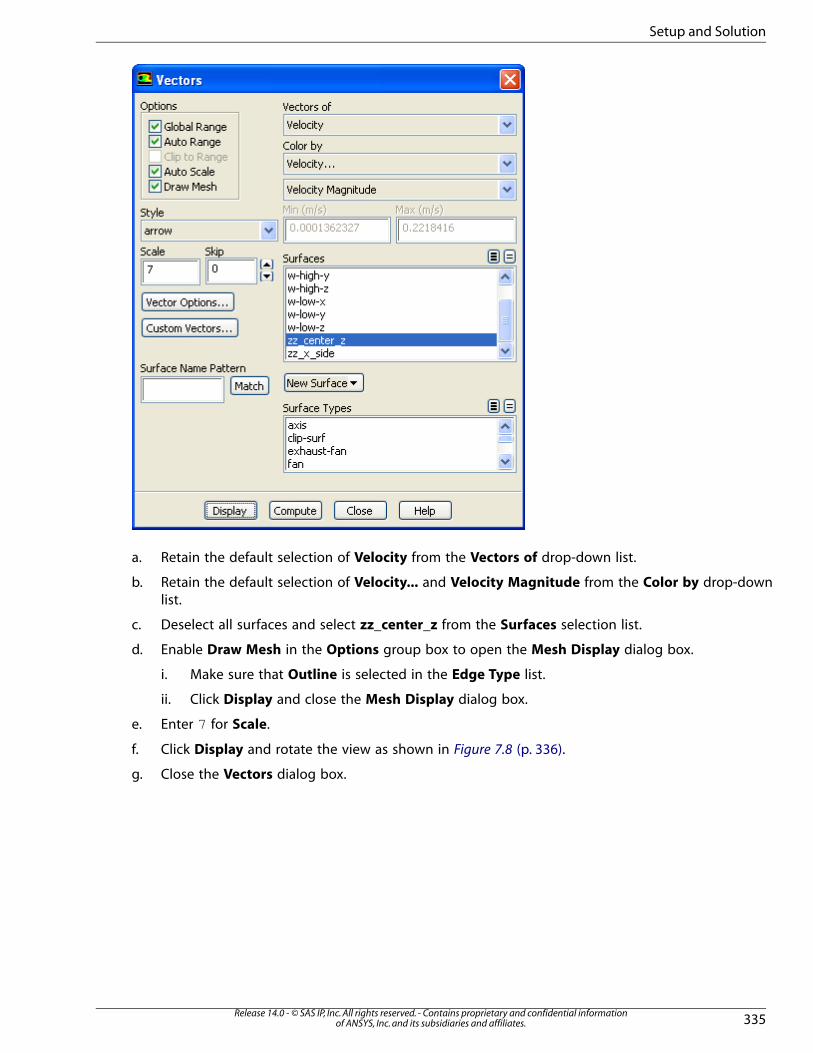
a. Retain the default selection of Velocity from the Vectors of drop-down list.

b. Retain the default selection of Velocity... and Velocity Magnitude from the Color by drop-down

list.

c. Deselect all surfaces and select zz_center_z from the Surfaces selection list.

d. Enable Draw Mesh in the Options group box to open the Mesh Display dialog box.

i. Make sure that Outline is selected in the Edge Type list.

ii. Click Display and close the Mesh Display dialog box.

e. Enter 7 for Scale.

f. Click Display and rotate the view as shown in Figure 7.8 (p. 336).

g. Close the Vectors dialog box.



Setup and Solution

Figure 7.8 Vectors of Velocity Magnitude

6. Compute view factors and radiation emitted from the front wall (w-high-x) to all other walls.

Report → S2S Information...



a. Make sure that View Factors is enabled in the Report Options group box.

b. Enable Incident Radiation.

c. Select w-high-x from the From selection list.

d. Select all zones except w-high-x from the To selection list.

e. Click Compute and close the S2S Information dialog box.

The computed values of the Views Factors and Incident Radiation are displayed in the console.

A view factor of approximately 0.2 for each wall is a good value for the square box.

7. Compute the total heat transfer rate.

Reports → Fluxes → Set Up...



Setup and Solution

a. Select Total Heat Transfer Rate in the Options group box.

b. Select all boundary zones except default-interior from the Boundaries selection list.

c. Click Compute.

Note

The energy imbalance is approximately 0.04%.

8. Compute the total heat transfer rate for w-low-x.


a. Retain the selection of Total Heat Transfer Rate in the Options group box.

b. Deselect all boundary zones and select w-low-x from the Boundaries selection list.

c. Click Compute.

Note

The net heat load is approximately 63 W.

9. Compute the radiation heat transfer rate.




a. Select Radiation Heat Transfer Rate in the Options group box.


c. Click Compute.

Note

The heat imbalance is approximately -0.014 W.

10. Compute the radiation heat transfer rate for w-low-x.




Setup and Solution

a. Retain the selection of Radiation Heat Transfer Rate in the Options group box.

b. Deselect all boundary zones and select w-low-x from the Boundaries selection list.

c. Click Compute and close the Flux Reports dialog box.

The net heat load is approximately 51 W. After comparing the total heat transfer rate and radiation

heat transfer rate, it can be concluded that radiation is the dominant mode of heat transfer.

11. Display temperature profile for the side wall.

Plots → XY Plot → Set Up...



a. Select Temperature... and Wall Temperature (Outer Surface) from the Y Axis Function drop-

down lists.

b. Retain the default selection of Direction Vector from the X Axis Function drop-down list.

c. Select zz_x_side from the Surfaces selection list.

d. Click Plot (Figure 7.9 (p. 341)).

e. Enable Write to File and click the Write... button to open the Select File dialog box.

i. Enter tp_1.xy for XY File.


f. Disable the Write to File option.

g. Close the Solution XY Plot dialog box.

Figure 7.9 Temperature Profile Along Outer Surface

12. Save the case and data files (rad_b_1.cas.gz and rad_b_1.dat.gz ).

File → Write → Case & Data...

7.4.9. Step 8: Compare the Contour Plots after Varying Radiating Surfaces

1. Increase the number of faces per cluster to 10.


a. Click on the Settings... button to open the View Factors and Clustering dialog box.

i. Enter 10 for Faces per Surface Cluster for Flow Boundary Zones in the Manual group box.



Setup and Solution

ii. Click Apply to All Walls and OK to close the View Factors and Clustering dialog box.

b. Click Compute/Write/Read... to open the Select File dialog box and to compute the view factors.

Specify a file name where the cluster and view factor parameters will be stored.

i. Enter rad_10.s2s.gz for S2S File.


c. Click OK to close the Radiation Model dialog box.



3. Start the calculation by requesting 300 iterations.

Run Calculation

The solution will converge in approximately 275 iterations.

4. Save the case and data files (rad_10.cas.gz and rad_10.dat.gz ).


5. In a manner similar to the steps described in Step 7: 11. (a)–(g), display the temperature profile for the

side wall and write it to a file named tp_10.xy .

6. Repeat the procedure outlined in Step 8: 1.–5. for 100, 400, 800, and 1600 faces per surface cluster and

save the respective case and data files (e.g., rad_100.cas.gz ) and temperature profile files (e.g.,

tp_100.xy ).

7. Display contours of wall temperature (outer surface) for all six cases, in the manner described in Step

7: 3.




Figure 7.10 Contours of Wall Temperature (Outer Surface): 1 Face per Surface Cluster



Setup and Solution

Figure 7.11 Contours of Wall Temperature (Outer Surface): 10 Faces per SurfaceCluster






Setup and Solution


8. Display contours of surface cluster ID for 1600 faces per surface cluster (Figure 7.16 (p. 350)).





b. Make sure that Node Values is disabled.

c. Select Radiation... and Surface Cluster ID from the Contours of drop-down lists.


e. Click Display and rotate the figure as shown in Figure 7.16 (p. 350).

f. Close the Contours dialog box.



Setup and Solution

Figure 7.16 Contours of Surface Cluster ID—1600 Faces per Surface Cluster (FPSC)

9. Read rad_400.cas.gz and rad_400.dat.gz and, in a similar manner to the previous step, display

contours of surface cluster ID (Figure 7.17 (p. 351)).



Figure 7.17 Contours of Surface Cluster ID—400 FPSC

Figure 7.17 (p. 351) shows contours of Surface Cluster ID for 400 FPSC. This case shows better clustering

compared to all of the other cases.

10. Create a plot that compares the temperature profile plots for 1, 10, 100, 400, 800, and 1600 FPSC.

Plots → File → Set Up...

a. Click Add... to open the Select File dialog box.

i. Select the file tp_1.xy that you created in Step 7: 11.

ii. Click OK to close the Select File dialog box.

b. Change the legend entry for the data series.



Setup and Solution

i. Enter Faces/Cluster in the Legend Title text box.

ii. Enter 1 in the text box to the left of the Change Legend Entry button.

iii. Click Change Legend Entry.

ANSYS FLUENT will update the Legend Entry text for the file tp_1.xy .

c. Repeat steps (a) and (b) to load the files tp_10.xy , tp_100.xy , tp_400.xy , tp_800.xy ,

and tp_1600.xy and change their Legend Entries accordingly.

d. Click Axes... to open the Axes dialog box.

i. Ensure X is selected in the Axis group box.

ii. Set Precision to 3 and click Apply.

iii. Select Y in the Axis group box.

iv. Set Precision to 2 and click Apply.

v. Close the Axes dialog box.



e. Click Plot (Figure 7.18 (p. 353)) and close the File XY Plot dialog box.

Figure 7.18 A Comparison of Temperature Profiles along the Outer Surface

7.4.10. Step 9: S2S Definition, Solution and Postprocessing with Partial Enclos-ure

As mentioned previously, when the S2S model is used, you also have the option to define a “partial enclosure”;

i.e., you can disable the view factor calculation for walls with negligible emission/absorption, or walls that

have uniform temperature. Even though the view factor will not be computed for these walls, they will still

emit radiation at a fixed temperature called the “partial enclosure temperature”. The main advantage of this

is to speed up the view factor and the radiosity calculation.

In the steps that follow, you will specify the radiating wall (w-low-x) as a boundary zone that is not particip-

ating in the S2S radiation model. Consequently, you will specify the partial enclosure temperature for the

wall. The partial enclosure option may not yield accurate results in cases that have multiple wall boundaries

that are not participating in S2S radiation and that each have different temperatures. This is because a single

partial enclosure temperature is applied to all of the non-participating walls.

1. Read the case file saved previously for the S2S model (rad_b_1.cas.gz ).

File → Read → Case...

2. Set the partial enclosure parameters for the S2S model.

Boundary Conditions → w-low-x → Edit...



Setup and Solution

a. Click the Radiation tab.

b. Disable Participates in View Factor Calculation in the S2S Parameters group box.

c. Click OK to close the Wall dialog box.

3. Compute the view factors for the S2S model.




a. Click Settings... to open View Factors and Clustering dialog box.

b. Click Select... to open Participating Boundary Zones dialog box.

i. Enter 473 K for Non-Participating Boundary Zones Temperature.

ii. Click OK to close Participating Boundary Zones dialog box.

c. Click OK to close View Factors and Clustering dialog box.

d. Click Compute/Write/Read... to open the Select File dialog box and to compute the view factors.

The view factor file will store the view factors for the radiating surfaces only. This may help you

control the size of the view factor file as well as the memory required to store view factors in

ANSYS FLUENT. Furthermore, the time required to compute the view factors will reduce as only

the view factors for radiating surfaces will be calculated.

Note

You should compute the view factors only after you have specified the boundaries

that will participate in the radiation model using the Boundary Conditions dialog

box. If you first compute the view factors and then make a change to the boundary

conditions, ANSYS FLUENT will use the view factor file stored previously for calcu-

lating a solution, in which case, the changes that you made to the model will not

be used for the calculation. Therefore, you should recompute the view factors and

save the case file whenever you modify the number of objects that will participate

in radiation.



Setup and Solution

i. Enter rad_partial.s2s.gz as the file name for S2S File.


e. Click OK to close the Radiation Model dialog box.



5. Start the calculation by requesting 300 iterations.

Run Calculation

The solution will converge in approximately 275 iterations.

6. Save the case and data files (rad_partial.cas.gz and rad_partial.dat.gz ).


7. Compute the radiation heat transfer rate.


a. Make sure that Radiation Heat Transfer Rate is selected in the Options group box.


c. Click Compute and close the Flux Reports dialog box.

8. Compare the temperature profile for the side wall to the profile saved in tp_1.xy .

Plots → XY Plot → Set Up...

a. Display the temperature profile and write it to a file named tp_partial.xy , in a manner similar

to the instructions shown in Step 7: 11.



b. Click the Load File... button to open the Select File dialog box.

i. Select tp_1.xy.

ii. Click OK to close the Select File dialog box.

c. Click Plot.

d. Close the Solution XY Plot dialog box.

Figure 7.19 Temperature Profile Comparison on Outer Surface

7.5. Summary

In this tutorial you studied combined natural convection and radiation in a three-dimensional square

box and compared the performance of surface-to-surface (S2S) radiation models in ANSYS FLUENT for

various radiating surfaces. The S2S radiation model is appropriate for modeling the enclosure radiative

transfer without participating media whereas the methods for participating radiation may not always

be efficient.

For more information about the surface-to-surface (S2S) radiation model, see Modeling Radiation in the

User’s Guide.

7.6. Further Improvements

This tutorial guides you through the steps to reach an initial solution. You may be able to obtain a more

accurate solution by using an appropriate higher-order discretization scheme and by adapting the mesh.

Mesh adaption can also ensure that the solution is independent of the mesh. These steps are demon-

strated in Introduction to Using ANSYS FLUENT: Fluid Flow and Heat Transfer in a Mixing Elbow (p. 131).



Further Improvements

chapter 7: modeling radiation and natural convection

Documents

warning dialog box

axis group box

options group box

manual group box

clustering dialog box

axes dialog box

free stream temperature

question dialog box