Chapter 7:

Going Nonlinear: Progressing Complexity

May 30, 2011

The early linear stages of structure formation have been succesfully and completely worked out withinthe context of the linear theory of gravitationally evolving cosmological density and perturbation fields(Peebles 1980). At every cosmologically interesting scale, it aptly and succesfully describes the situationin the early eons after the decoupling of radiation and matter at recombination. It still does so at presenton those spatial scales at which the landscape of spatially averaged perturbations resembles a panoramaof gently sloping hills. However, linear theoretical predictions soon fail after gravity surpasses its initialmoderate impact and nonlinear features start to emerge. Soon thereafter, we start to distinguish thegradual rise of the complex patterns, structures and objects which have shaped our Universe into thefascinating world of astronomy.

Once the evolution is entering a stage in which the first nonlinearities start to mature, it is no longerfeasible to decouple the growth of structure on the various involved spatial and mass scales. Rapidlymaturing small scale clumps do feel the effect of the large scale environment in which they are embedded.Neighbouring structures not only influence each other by external long-range gravitational forces butalso by their impact on resulting matter flows. The morphology and topology of more gradually forminglarge-scale features will depend to a considerable extent on the characteristics of their content in smallerscale structures that were formed earlier on. This never-ending increasing level of complexity has provedto pose a daunting challenge for developing a fully consistent theoretical framework. No cosmogenictheory as yet has managed to integrate all acquired insights and observed impressions of the worldaround us.

1. Nonlinear Evolution: Mode Coupling

Once density perturbations become of the order unity, δ(x, t) ≈ 1, it is no longer possible to use thebasic linear theory of clustering. Different modes of the density fields will start to interact, resulting inmutual “power transfer”.

Restricting ourselves to a pure matter-dominated Universe, the full nonlinear fluid evolution equationswere (see chapter 4),

∂δ

∂t+

1

a~∇x · (1 + δ)~v = 0

∂~v

∂t+

1

a

(~v · ~∇x

)~v +

a

a~v = −

1

a~∇xφ (1)

∇2xφ = 4πGa2 ρu δ

1

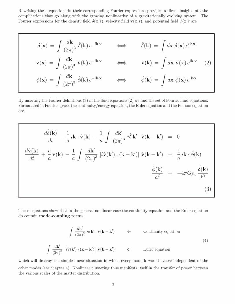
Rewriting these equations in their corresponding Fourier expressions provides a direct insight into thecomplications that go along with the growing nonlinearity of a gravitationally evolving system. TheFourier expressions for the density field δ(x, t), velocity field v(x, t), and potential field φ(x, t are

δ(x) =

∫dk

(2π)3 δ(k) e−ik·x ⇐⇒ δ(k) =

∫dx δ(x) eik·x

v(x) =

∫dk

(2π)3 v(k) e−ik·x ⇐⇒ v(k) =

∫dx v(x) eik·x (2)

φ(x) =

∫dk

(2π)3 φ(k) e−ik·x ⇐⇒ φ(k) =

∫dx φ(x) eik·x

By inserting the Fourier definitions (3) in the fluid equations (2) we find the set of Fourier fluid equations.Formulated in Fourier space, the continuity/energy equation, the Euler equation and the Poisson equationare

dδ(k)

dt−

1

aik · v(k) −

1

a

∫dk′

(2π)3 iδ k′ · v(k − k′) = 0

dv(k)

dt+a

av(k) −

1

a

∫dk′

(2π)3 [iv(k′) · (k − k′)] v(k − k′) =1

aik · φ(k)

φ(k)

a2 = −4πGρuδ(k)

k2

(3)

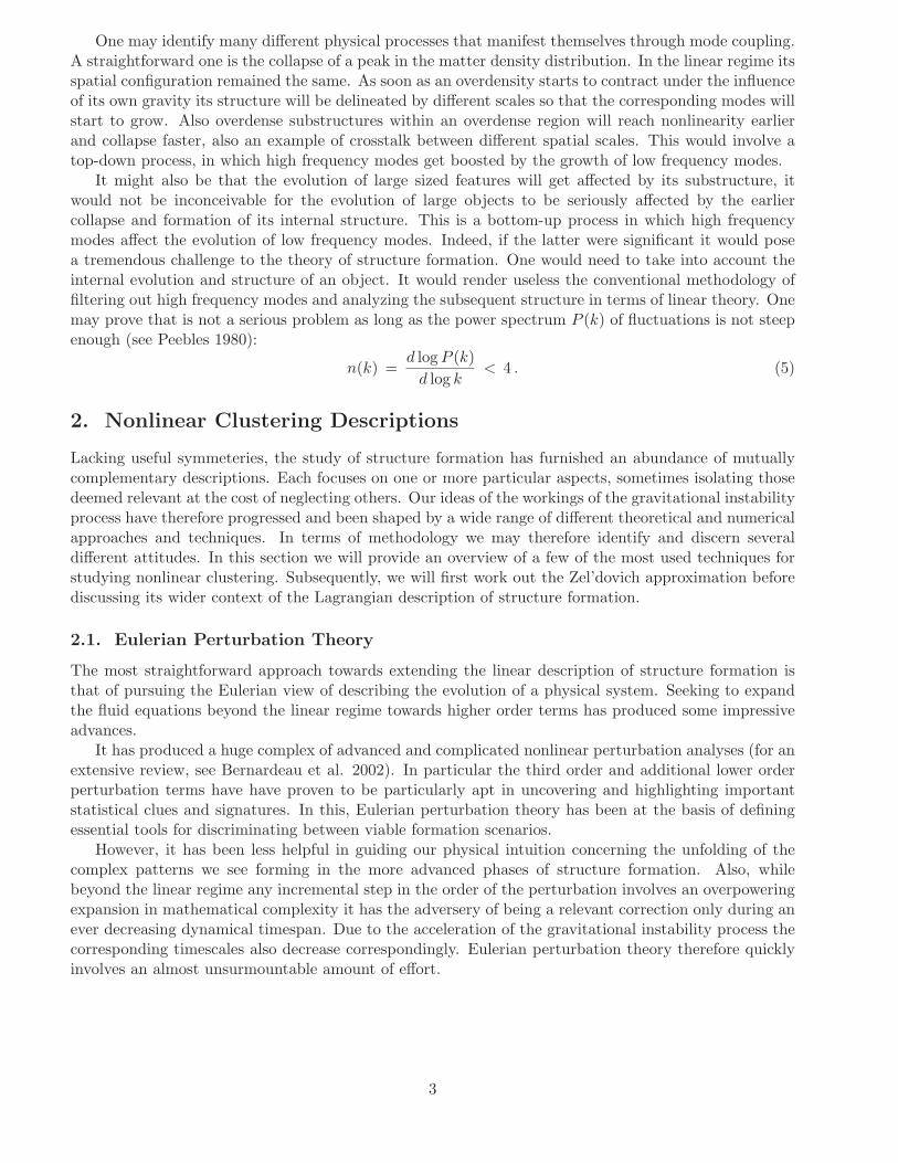
These equations show that in the general nonlinear case the continuity equation and the Euler equationdo contain mode-coupling terms,

∫dk′

(2π)3iδ k′ · v(k − k′) ⇐ Continuity equation

(4)∫

dk′

(2π)3[iv(k′) · (k − k′)

]v(k − k′) ⇐ Euler equation

which will destroy the simple linear situation in which every mode k would evolve independent of the

other modes (see chapter 4). Nonlinear clustering thus manifests itself in the transfer of power betweenthe various scales of the matter distribution.

2

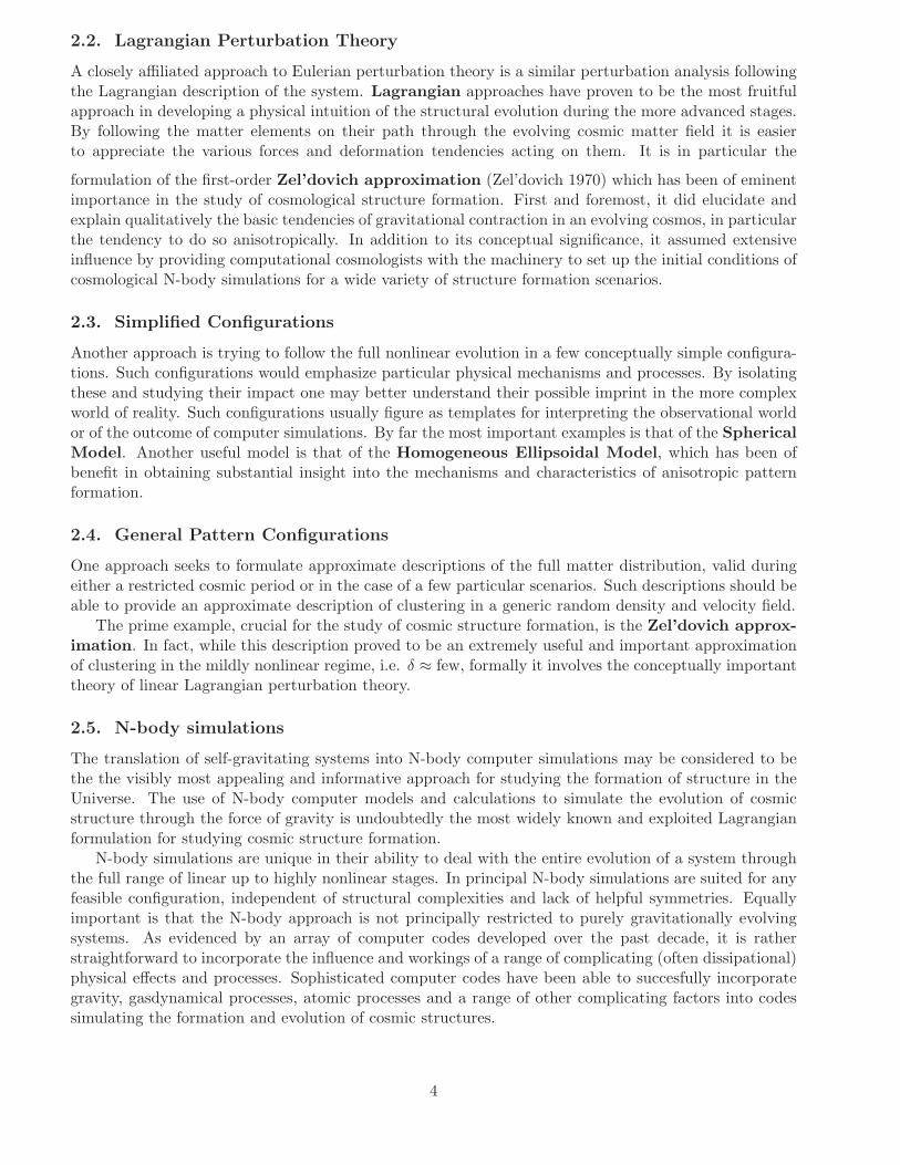
One may identify many different physical processes that manifest themselves through mode coupling.A straightforward one is the collapse of a peak in the matter density distribution. In the linear regime itsspatial configuration remained the same. As soon as an overdensity starts to contract under the influenceof its own gravity its structure will be delineated by different scales so that the corresponding modes willstart to grow. Also overdense substructures within an overdense region will reach nonlinearity earlierand collapse faster, also an example of crosstalk between different spatial scales. This would involve atop-down process, in which high frequency modes get boosted by the growth of low frequency modes.

It might also be that the evolution of large sized features will get affected by its substructure, itwould not be inconceivable for the evolution of large objects to be seriously affected by the earliercollapse and formation of its internal structure. This is a bottom-up process in which high frequencymodes affect the evolution of low frequency modes. Indeed, if the latter were significant it would posea tremendous challenge to the theory of structure formation. One would need to take into account theinternal evolution and structure of an object. It would render useless the conventional methodology offiltering out high frequency modes and analyzing the subsequent structure in terms of linear theory. Onemay prove that is not a serious problem as long as the power spectrum P (k) of fluctuations is not steepenough (see Peebles 1980):

n(k) =d logP (k)

d log k< 4 . (5)

2. Nonlinear Clustering Descriptions

Lacking useful symmeteries, the study of structure formation has furnished an abundance of mutuallycomplementary descriptions. Each focuses on one or more particular aspects, sometimes isolating thosedeemed relevant at the cost of neglecting others. Our ideas of the workings of the gravitational instabilityprocess have therefore progressed and been shaped by a wide range of different theoretical and numericalapproaches and techniques. In terms of methodology we may therefore identify and discern severaldifferent attitudes. In this section we will provide an overview of a few of the most used techniques forstudying nonlinear clustering. Subsequently, we will first work out the Zel’dovich approximation beforediscussing its wider context of the Lagrangian description of structure formation.

2.1. Eulerian Perturbation Theory

The most straightforward approach towards extending the linear description of structure formation isthat of pursuing the Eulerian view of describing the evolution of a physical system. Seeking to expandthe fluid equations beyond the linear regime towards higher order terms has produced some impressiveadvances.

It has produced a huge complex of advanced and complicated nonlinear perturbation analyses (for anextensive review, see Bernardeau et al. 2002). In particular the third order and additional lower orderperturbation terms have have proven to be particularly apt in uncovering and highlighting importantstatistical clues and signatures. In this, Eulerian perturbation theory has been at the basis of definingessential tools for discriminating between viable formation scenarios.

However, it has been less helpful in guiding our physical intuition concerning the unfolding of thecomplex patterns we see forming in the more advanced phases of structure formation. Also, whilebeyond the linear regime any incremental step in the order of the perturbation involves an overpoweringexpansion in mathematical complexity it has the adversery of being a relevant correction only during anever decreasing dynamical timespan. Due to the acceleration of the gravitational instability process thecorresponding timescales also decrease correspondingly. Eulerian perturbation theory therefore quicklyinvolves an almost unsurmountable amount of effort.

3

2.2. Lagrangian Perturbation Theory

A closely affiliated approach to Eulerian perturbation theory is a similar perturbation analysis followingthe Lagrangian description of the system. Lagrangian approaches have proven to be the most fruitfulapproach in developing a physical intuition of the structural evolution during the more advanced stages.By following the matter elements on their path through the evolving cosmic matter field it is easierto appreciate the various forces and deformation tendencies acting on them. It is in particular the

formulation of the first-order Zel’dovich approximation (Zel’dovich 1970) which has been of eminentimportance in the study of cosmological structure formation. First and foremost, it did elucidate andexplain qualitatively the basic tendencies of gravitational contraction in an evolving cosmos, in particularthe tendency to do so anisotropically. In addition to its conceptual significance, it assumed extensiveinfluence by providing computational cosmologists with the machinery to set up the initial conditions ofcosmological N-body simulations for a wide variety of structure formation scenarios.

2.3. Simplified Configurations

Another approach is trying to follow the full nonlinear evolution in a few conceptually simple configura-tions. Such configurations would emphasize particular physical mechanisms and processes. By isolatingthese and studying their impact one may better understand their possible imprint in the more complexworld of reality. Such configurations usually figure as templates for interpreting the observational worldor of the outcome of computer simulations. By far the most important examples is that of the SphericalModel. Another useful model is that of the Homogeneous Ellipsoidal Model, which has been ofbenefit in obtaining substantial insight into the mechanisms and characteristics of anisotropic patternformation.

2.4. General Pattern Configurations

One approach seeks to formulate approximate descriptions of the full matter distribution, valid duringeither a restricted cosmic period or in the case of a few particular scenarios. Such descriptions should beable to provide an approximate description of clustering in a generic random density and velocity field.

The prime example, crucial for the study of cosmic structure formation, is the Zel’dovich approx-imation. In fact, while this description proved to be an extremely useful and important approximationof clustering in the mildly nonlinear regime, i.e. δ ≈ few, formally it involves the conceptually importanttheory of linear Lagrangian perturbation theory.

2.5. N-body simulations

The translation of self-gravitating systems into N-body computer simulations may be considered to bethe the visibly most appealing and informative approach for studying the formation of structure in theUniverse. The use of N-body computer models and calculations to simulate the evolution of cosmicstructure through the force of gravity is undoubtedly the most widely known and exploited Lagrangianformulation for studying cosmic structure formation.

N-body simulations are unique in their ability to deal with the entire evolution of a system throughthe full range of linear up to highly nonlinear stages. In principal N-body simulations are suited for anyfeasible configuration, independent of structural complexities and lack of helpful symmetries. Equallyimportant is that the N-body approach is not principally restricted to purely gravitationally evolvingsystems. As evidenced by an array of computer codes developed over the past decade, it is ratherstraightforward to incorporate the influence and workings of a range of complicating (often dissipational)physical effects and processes. Sophisticated computer codes have been able to succesfully incorporategravity, gasdynamical processes, atomic processes and a range of other complicating factors into codessimulating the formation and evolution of cosmic structures.

4

Figure 1. A mosaic of 4 blow-ups from a 2563 particle simulation by the Virgo consortium, correspondingto a SCDM scenario mass distribution at z = 0. Courtesy: VIRGO/Colberg et al.

5

However, the success and visual appeal of N-body simulations often also lead to overinterpretation.Many scientific studies unjustifiably ignore the limitations and artefacts of the computer calculations.Even the word “simulation” already carries with it the pretention of the computer models representingreality. It would be more honest, as well as modest, to talk about “computer experiments”. Also, anattitude has developed in which the reproduction of observed patterns or results by a computer modelis considered to be an explanation in itself. This is far from true, the computer models should be usedas mere guidelines. A true physical understanding may at best only start or be guided by computerexperiments.

3. Lagrangian Perturbation Theory

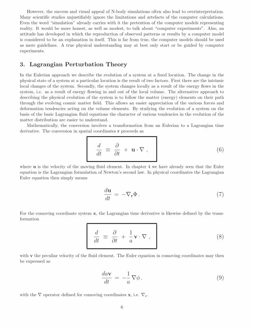
In the Eulerian approach we describe the evolution of a system at a fixed location. The change in thephysical state of a system at a particular location is the result of two factors. First there are the intrinsiclocal changes of the system. Secondly, the system changes locally as a result of the energy flows in thesystem, i.e. as a result of energy flowing in and out of the local volume. The alternative approach todescribing the physical evolution of the system is to follow the matter (energy) elements on their paththrough the evolving cosmic matter field. This allows an easier appreciation of the various forces anddeformation tendencies acting on the volume elements. By studying the evolution of a system on thebasis of the basic Lagrangian fluid equations the character of various tendencies in the evolution of thematter distribution are easier to understand.

Mathematically, the conversion involves a transformation from an Eulerian to a Lagrangian timederivative. The conversion in spatial coordinates r proceeds as

d

dt≡

∂

∂t+ u · ∇ , (6)

where u is the velocity of the moving fluid element. In chapter 4 we have already seen that the Eulerequation is the Lagrangian formulation of Newton’s second law. In physical coordinates the LagrangianEuler equation then simply means

du

dt= −∇rΦ . (7)

For the comoving coordinate system x, the Lagrangian time derivative is likewise defined by the trans-formation

d

dt≡

∂

∂t+

1

av · ∇ , (8)

with v the peculiar velocity of the fluid element. The Euler equation in comoving coordinates may thenbe expressed as

dav

dt= −

1

a∇φ . (9)

with the ∇ operator defined for comoving coordinates x, i.e. ∇x.

6

3.1. Evolution and Deformation: Lagrangian View

As a given patch of matter participates in the evolution of the matter distribution it will evolve. Inits totality it will flow along a path defined by the forces it experiences. Its density will change as itgets compressed or as it expands. Shearing flows, in a gravitational system the result of tidal forces, willdeform the shape of the patch.

In the Lagrangian formulation the description of the deformation of a given fluid element is of centralimportance. It is straightforward to see that the deformations are closely linked to the flow field in andaround the fluid element. The various components of the deformation of the evolving mass element atcomoving location x are therefore encoded in the decomposition of the gradient of its velocity field v(the rate-of-strain tensor).

3.1.1. Expansion, Vorticity and Shear

We can distinguish three different modes, the expansion/compression θ, the shear σij and the vor-ticity tensor elements ωij , which contribute to the velocity deformation tensor vi,j as

1

a

∂vi

∂xj=

1

3θ δij + σij + ωij , (10)

in which the expansion θ is the trace of the velocity field gradient, σij = σji the traceless symmetric partand ωij = −ωji the antisymmetric part (and ǫijk the Levi-Civita symbol),

θ =1

a∇ · v ≡

1

a

(∂v1

∂x1+∂v2

∂x2+∂v3

∂x3

)

σij ≡1

2a

(∂vi

∂xj+∂vj

∂xi

)−

1

3(∇ · v) δij (11)

ωij ≡1

2a

(∂vi

∂xj−∂vj

∂xi

)

The vorticity tensor ωij is related to the vorticity ~ω of the fluid through the relations

ωij = ǫijkωk

(12)

~ω =1

2a∇× v

with ǫijk the three-dimensional Levi-Civita symbol. Notice that we transformed from physical coordi-nates r to comoving coordinates x, and from the full velocity u to the peculiar velocity v. This we caneasily do as the global Hubble expansion is a pure expansion (or compression) flow, only and exclusivelyinvolving a global velocity divergence ΘH ,

ΘH = 3H(t) (13)

7

so that we may easily transform to the comoving velocity deformation quantities by subtracting ΘH

from the full velocity divergence Θ,Θ = θ + 3H(t) . (14)

These quantities describe the change of a mass element during the evolution of a system. The expansion

term θ describes its expansion or contraction. It is the one component responsible for the change indensity (see next subsection). The shear tensor σij describes the change in shape of the matter element.By diagonalizing the shear tensor matrix σij we can infer the principal axes for the shape change fromthe direction of the eigenvectors while the eigenvalues describe the strength of this shape deformationalong each of the principal axes. The last factor of change that may affect the fluid element is rotationsdue to the presence of a vorticity term, ωij .

3.1.2. Lagrangian fluid equations

With the tools to describe the changing volume of the mass element whose evolution is followed by theLagrangian description, we can infer the equations that describe its evolution. The formalism whichwe will present here is based on two implicit restrictions. First, we will assume pure laminar flow andfollow fluid elements as long as they have not crossed the paths of other fluid elements. This allows usto limit outselves to a pure local description by focussing on the evolution of individual fluid elements.Secondly, we will restrict ourselves to a pressureless, purely gravitational system and ignore the influenceof pressure forces.

In the Eulerian formalism we described the evolution of the system in terms of comoving space, andwithin the same context of density and velocity perturbations against the background of an expandingUniverse we follow the same strategy to unfold a Lagrangian description of the evolving perturbations.

While the Eulerian description is focussing on the local change of perturbation quantities, and dealswith a constant (infinitesimal) volume element at a fixed (comoving) location x the Lagrangian descrip-tion has the additional need to describe the deformation of a particular volume element. Its volume willchange as it expands or contracts. Meanwhile generically also its shape and orientation will change whileflowing along space. It will therefore not be sufficient to just describe the change of the density excessor deficit δ, the accompanying peculiar velocity and gravitational potential. A proper and completedescription will have to address the development of the expansion/contraction θ, shear σij and rotationωij of the fluid element. These deforming tendencies will in turn affect density, velocity and potential.A complete Lagrangian formulation should therefore consist of more equations than the Eulerian set ofequations.

In total there are seven equations. One equation concerns the definition of the peculiar velocity v ofthe fluid element. Subsequently we have the Lagrangian equivalents of the three Eulerian fluid equations,the continuity equation for ensuring mass conservation, Newton’s second law as the Lagrangian equivalentof the Euler equation and the Poisson equation. In addition we need to account for the evolution ofthe expansion/contraction θ, which in turn is affected by the shear σij and vorticity ωij . For a fullcharacterization one therefore also needs the equations for the evolution of the shear and vorticity.

The first equation is rather straightforward and merely involves the definition of the peculiar velocityv(x, t),

v ≡ adx

dt=

dx

dτ. (15)

in which the conformal time τ ,

dτ =dt

a(16)

8

is used as the time derivative in the right expression. The first evolution equation to consider is the La-

grangian continuity/energy equation, expressing the conservation of mass/energy of the fluid element.A change in density is a result of the expansion or contraction of the volume of the fluid element. Whilethe Eulerian description looks at a fixed volume element and has to take account of the inflowing andoutflowing flux of energy, the Lagrangian view is that of a fluid element of a fixed mass/energy contentand changing density contrast δ as the result of the expansion/contraction θ of its volume,

dδ

dt+ a (1 + δ) θ = 0 (17)

The equation of motion of the fluid element – the Euler equation – can be directly inferred from itsEulerian version,

∂v

∂t+

1

a(v · ∇) v +

a

av = −

1

a∇φ (18)

and the expression for the translation from a comoving Eulerian to a comoving Lagrangian for-mulation, eqn. (8),

dv

dt= −

a

av −

1

a∇φ

In a more compact and direct notation this becomes

dav

dt= ∇φ . (19)

from which we can directly infer that in the absence of a source potential φ the peculiar velocity v ofthe fluid element rapidly decays away,

v ∝1

a. (20)

A similar conclusion had already been found for the peculiar velocity in the linear regime, for the strictlyEulerian case. For linking the force sourceterm – the potential φ – to the matter distribution theexpression in the Lagrangian formalism is the same as that for the Eulerian formalism. In other words,we retain the same Poisson Equation,

∇2φ = 4πGa2 ρu δ (21)

Upon assessing the above set of three Lagrangian fluid equations, we find that they include the explicitvelocity divergence term θ, the trace of ∇ivj . While one might evaluate θ by explicitly solving for v,a better approach is to use an explicit expression for the evolution of θ. This is the Raychaudhuryequation,

dθ

dt+ 2

a

aθ +

1

3θ2 + σijσij − 2~ω2 = −4πGρuδ (22)

9

The Raychaudhury equation follows from an evaluation of the Euler fluid equation (19) in combinationwith the Poisson equation (21).

The Raychaudhury equation introduces an interesting new element to our evaluations of an evolvingmatter distribution. Through the quadratic shear term σijσij and the quadratic vorticity term2~ω2 = ωijωij it includes an explicit term for the influence of shear on the evolution of fluid elements.Two observations may be made immediately. First, the shear and vorticity term appear to act like asource term, be it with opposite signs. The presence of shear accelerates the evolution of mass elements:while

dθ

dt∝ −σijσij , (23)

any presence of shear translates into an increase of the compression of a fluid element as θ tends to turnmore negative. The reverse influence is that of vorticity. Because

dθ

dt∝ ~ω2 , (24)

the presence of vorticity will oppose any collapsing tendency and instead tend to promote the expansionof a fluid element. Secondly, the influence of shear and vorticity is propragated via a quadratic terms,which means that they it involves pure nonlinear effects. During the linear regime the influenceof shear and vorticity is negligible. It had indeed not been observed to play a significant, modifying,influence in the treatment of linear structure evolution.

With the introduction of the shear and vorticity term as significant evolutionary influences we willalso have to consider their evolution in order to formulate a closed, complete, system of equations forthe evolution of the mass distribution.

The Lagrangian Vorticity equation describes the evolution of the vorticity ~ω of a fluid element.It follows from an evaluation of the antisymmetric part of the Euler equation, in combination with thecontinuity equation.

dωi

dt+ 2

a

aωi +

2

3θ ωi − σij ω

j = 0 (25)

This expression shows that if there is no primordial vorticity, i.e. if ~ω = 0, then the flow remains vorticityfree. This confirms the earlier assessment in the linear regime. This of course remains valid up to thelimitation of the Lagrangian description presented here. When flows are no longer laminar and start tocross the situation gets more complex and vorticity may be generated.

For the evolution of the shear σij the Lagrangian Shear equation can be derived from the sym-metric part of the Euler equation, in combination with the continuity equation,

dσij

dt+ 2

a

aσij +

2

3θ σij + σik σ

kj −

1

3δij (σklσkl) = −Tij (26)

where Tij is the gravitational tidal field working on the fluid element,

Tij(x) =1

a2

∂2φ

∂xi∂xj−

1

3∇2φ δij

. (27)

Within the context of general relativity Tij is the electric part of the Weyl tensor in the fluid frame.

As expected this equation is an expression of how the gravitational tidal field acts as a source term forinducing a shear component in the flow field. To be able to evaluate the value of Tij we need the Poissonequation for computing the gravitational potential field.

10

3.1.3. Irrotational flow

In our discussion of the linear regime we had noticed that in the case of a pressureless, purely gravita-tionally evolving system primordial vorticity will decay during linear evolution. This conclusion may beextrapolated towards the nonlinear regime. The Lagrangian vorticity equation (25) shows that ifa primordial fluid element is irrotational it will remain so during its further nonlinear evolution (up tostreamlines crossing).

Under the assumption that the fluid is pressureless and irrotational (i.e. ωi = 0), the evolution of afluid element – with comoving trajectory x(t) – is specified by six first order differential equations. Insummary, the complete set of irrotational Lagrangian fluid equations is:

v = adx

dtdv

dt+a

av = −

1

a∇φ

dδ

dt+ (1 + δ) θ = 0

dθ

dt+ 2

a

aθ +

1

3θ2 + σijσij = −4πGρuδ

(28)dσij

dt+a

aσij +

2

3θ σij + σik σ

kj −

1

3δij (σklσkl) = −Tij

∇2xφ = 4πGa2 ρu δ

Tij(x) =1

a2

∂2φ

∂xi∂xj−

1

3∇2φ δij

3.1.4. Lagrangian collapse

An interesting observation follows from evaluating the combination of the continuity and Raychaudhuriequation. It leads to a second order ordinary differential equation describing the evolution of the densitycontrast δ of a fluid element:

d2δ

dt2+ 2

a

a

dδ

dt=

4

3(1 + δ)−1

(dδ

dt

)2

+ (1 + δ)

(2

3σijσij − 2~ω2 + 4πGρuδ

)

(29)

11

Bertschinger & Jain (1994) noted that this equation shows that in the absence of vorticity the presenceof a nonzero shear increases the rate of growth of density fluctuations (vorticity will inhibit this process).In other words, the rate of growth of δ gets amplified in the presence of shear. This conclusion holdsindependently of assumptions about the evolution of shear or tides and is due to the simple geometricalfact that shear increases the rate of growth of the convergence (∝ −θ) of fluid streamlines.

With zero shear and vorticity the velocity gradient tensor is isotropic, corresponding to uniformspherical collapse with radial motions towards some centre (see sect. (??). Equation (29) then reducesto the exact equation for the evolution of the mean density in the spherical model,

d2δ

dt2+ 2

a

a

dδ

dt=

4

3(1 + δ)−1

(dδ

dt

)2

+ 4πGρuδ(1 + δ) (30)

An important and immediate observation is that this implies the growth of uniform spherical perturba-tions to be more slowly than more generic anisotropic configurations with a nonzero shear term:

Shear streaming accelerates Collapse:

⇐⇒

Spherical Collapse is slowest !!!

EXERCISE: Derive expression (30) for the evolution of the density δ(r, t) of a shell in the sphericalmodel. Note: use the equations for the spherical model in section (5).

3.1.5. Localized Lagrangian Approximations

Careful consideration of the first three fluid equations shows that the Lagrangian description entailsa nearly exclusive local view of the evolution of the matter distribution. All quantities relate to the“local” values pertaining to one particular piece of matter.

The one remaining complication for transforming the Lagrangian fluid equations into such local

descriptions involves the development of the driving shear term σij . Evidently, its evolution dependson the behaviour of the gravitational tide Tij . Obviously, its value is generically determined by the fullmatter distribution throughout the cosmic volume. Ultimately, the one non-local ingredient is that ofthe gravitational field, involving contributions from all over space. There have been various attemptsto circumvent these non-local complications by developing approximate schemes for the evolution of thegravitational field.

The locality of these approximation schemes implies the evolution to be described by a set of ordinary

differential equations for each mass element, with no coupling to other mass elements aside from thoseimplied by the initial conditions. Note that N-body simulations are distinctly non-local Lagrangiandescriptions. At every timestep the full gravitational potential set by the full cosmic matter distributionneeds to be evaluated at the location of every mass element.

We will see that the Zel’dovich approximation (1970) is the most succesfull representative of aclass of Lagrangian approximation schemes in which the nonlinear dynamics of selfgravitating matter isencapsulated into an approximate “local” formulation (Bertschinger & Jain 1994, Hui & Bertschinger1996). In these localized Lagrangian approaches, the density, velocity gradient, and gravity gradientfor each mass element behaves as if the element evolves independently of all the others once the initialconditions are specified. For instance, the evolution of a given mass element under the Zel’dovichapproximation is completely determined once the initial expansion, vorticity, shear and density at this

12

mass element are specified. The influence of other mass elements on the subsequent evolution of thesequantities at this particular mass element is then assumed to be fully encoded in the initial conditions,and unaffected by the subsequent evolution of these other mass elements. Such a presumption may seemimplausible in view of the unrestrained long-range gravitational force, yielding a noticeable influencefrom all other mass elements in the Universe.

Yet, the success of the Zel’dovich approximation, having provided a great deal of insight into theessentials of nonlinear evolution of density fluctuations, demonstrates how useful such schemes in factcan be.

4. Zel’dovich Approximation

By means of a Lagrangian perturbation analysis Zel’dovich (1970) proved, in a seminal contribution,that to first order – typifying early evolutionary phases – the reaction of cosmic patches of matter tothe corresponding peculiar gravity field would be surprisingly simple. The resulting expression involvesa plain ballistic linear displacement set solely by the initial (Lagrangian) force field. It frames thewell-known Zel’dovich approximation.

The essence of the Lagrangian formalism is a mapping from the initial comoving position q of a masselement onto its location x(q, t):

q −→ x(q, t) (31)

The initial comoving location q is the Lagrangian coordinate of the matter element, and will be used as a“tag” to identify it while moving along its path x(q). Of course the Lagrangian coordinate of each masselement remains the same throughout cosmic time. The Lagrangian perturbation formalism describesthe displacement

s ≡ x − q (32)

of a mass element in terms of an ordered sequence of moments of displacement,

x(q, t) = q + x(1)(q, t) + x(2)(q, t) + . . . (33)

in which the successive terms xm correspond to successive terms of the relative displacement |∂(x −q)/∂q|,

1 ≫

∣∣∣∣∣∂x(1)

∂q

∣∣∣∣∣ ≫∣∣∣∣∣∂x(2)

∂q

∣∣∣∣∣ ≫∣∣∣∣∣∂x(3)

∂q

∣∣∣∣∣ ≫ . . . (34)

The Zel’dovich approximation is the solution of the Lagrangian fluid equations for small density pertur-bations (δ2 ≪ 1), corresponding to a solution for its displacement s truncated at the first order x(1) inthe above Lagrangian perturbation series. The Zel’dovich approximation thus corresponds to a simplelinear prescription for the displacement of a particle.

4.0.6. Zel’dovich Mapping and Density Evolution

Given the mapping from the Lagrangian coordinate q to the Eulerian coordinate x, we may infer thedensity evolution induced by the displacement of the mass by the demand of mass conservation.The mass originally contained in an infinitesimal volume dq is transported to the infinitesimal volumedx. The density in Lagrangian space q is of course equal to the average cosmic density at time t, ρu(t).On the basis of mass conservation within we then find that the density at position x in Eulerian space is

ρ(x, t) dx = ρu(t) dq (35)

13

so that we find that the density perturbation δ(x, t) is

1 + δ(x, t) =ρ(x, t)

ρu(t)=

∥∥∥∥∥∂x

∂q

∥∥∥∥∥

−1

(36)

with ‖ · · · ‖ the Jacobian determinant.

4.0.7. Lagrangian Perturbation theory

To compute the Jacobian determinant 36) in terms of the Lagrangian perturbation series, we take theJacobian from the expression (33) for the displacement (x − q),

∂x

∂q= 1 +

∂x(1)

∂q+∂x(2)

∂q+ · · ·

≈

1 +∂x

(1)1

∂q1

∂x(1)2

∂q1

∂x(1)3

∂q1

∂x(1)1

∂q21 +

∂x(1)2

∂q2

∂x(1)3

∂q2

∂x(1)1

∂q3

∂x(1)2

∂q31 +

∂x(1)3

∂q3

(37)

In this 1 is the identity matrix. To first order the Jacobian determinant can therefore be written as

∥∥∥∥∥∂x

∂q

∥∥∥∥∥ ≈

(1 +

∂x(1)1

∂q1

) (1 +

∂x(1)2

∂q2

) (1 +

∂x(1)3

∂q3

)+ · · ·

(38)

≈ 1 + ∇q · x(1) + O(· · · ) (39)

Using this result we then obtain the first order approximation for the density perturbation, δ(1)(x, t), byinserting the first order expression for the Jacobian matrix in eqn. (36),

δ(1)(x, t) = −∇q · x(1) (40)

This relation between density perturbation δ(1) and displacement x(1) allows us to infer a relation betweenthe primordial potential perturbation φ(1) and x(1) via the Poisson equation,

∇2φ(1) = 4πGρu a2 δ(1) = −4πGρu a

2 ∇q · x(1) . (41)

14

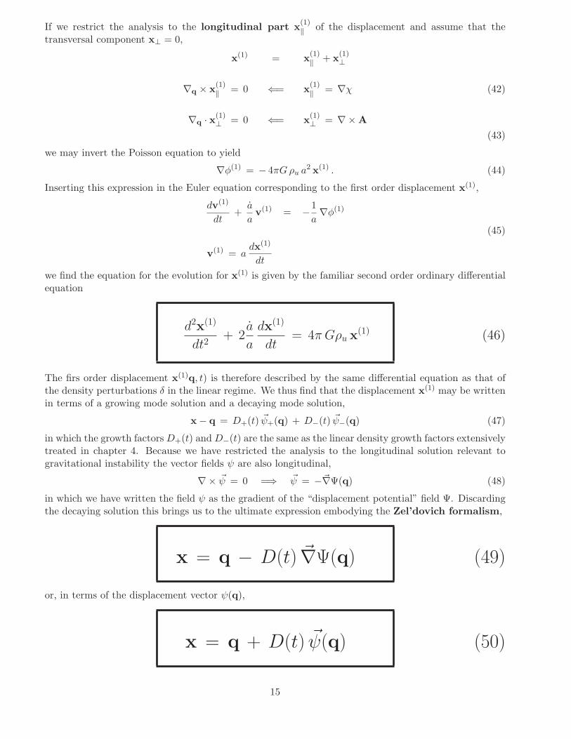
If we restrict the analysis to the longitudinal part x(1)‖ of the displacement and assume that the

transversal component x⊥ = 0,

x(1) = x(1)‖ + x

(1)⊥

∇q × x(1)‖ = 0 ⇐= x

(1)‖ = ∇χ (42)

∇q · x(1)⊥ = 0 ⇐= x

(1)⊥ = ∇× A

(43)

we may invert the Poisson equation to yield

∇φ(1) = − 4πGρu a2 x(1) . (44)

Inserting this expression in the Euler equation corresponding to the first order displacement x(1),

dv(1)

dt+a

av(1) = −

1

a∇φ(1)

(45)

v(1) = adx(1)

dt

we find the equation for the evolution for x(1) is given by the familiar second order ordinary differentialequation

d2x(1)

dt2+ 2

a

a

dx(1)

dt= 4π Gρu x(1) (46)

The firs order displacement x(1)q, t) is therefore described by the same differential equation as that ofthe density perturbations δ in the linear regime. We thus find that the displacement x(1) may be writtenin terms of a growing mode solution and a decaying mode solution,

x − q = D+(t) ~ψ+(q) + D−(t) ~ψ−(q) (47)

in which the growth factorsD+(t) andD−(t) are the same as the linear density growth factors extensivelytreated in chapter 4. Because we have restricted the analysis to the longitudinal solution relevant togravitational instability the vector fields ψ are also longitudinal,

∇× ~ψ = 0 =⇒ ~ψ = −~∇Ψ(q) (48)

in which we have written the field ψ as the gradient of the “displacement potential” field Ψ. Discardingthe decaying solution this brings us to the ultimate expression embodying the Zel’dovich formalism,

x = q − D(t) ~∇Ψ(q) (49)

or, in terms of the displacement vector ψ(q),

x = q + D(t) ~ψ(q) (50)

15

4.0.8. Zel’dovich formalism: Peculiar Velocity

From the Zel’dovich equation (50) we may readily evaluate the peculiar velocity of the fluid element withLagrangian coordinate q:

v = adx

dt= − aD ~∇Ψ

= − aDHa D

aD~∇Ψ (51)

yielding the expression

v = − aDHf(Ω) ~∇Ψ (52)

This, in turn, allows us to relate the “displacement potential” Ψ to the gravitational potential perturba-tion φ. We know that in the linear regime the peculiar velocity v is directly proportional to the peculiargravity g,

v =2f(Ω)

3ΩHg = −

2f(Ω)

3ΩH

∇φ

a(53)

Equating expression (53) to its Zel’dovich equivalent (52) enables us to immediately find the intendedrelation:

Ψ(q) =2

3Da2H2 Ωφ(x, t) (54)

As a consistency dheck we may notice that this implies the potential Ψ to be time-independent. Becauseaccording to linear theory the gravitational potential φ grows as

φ(t) =D

aφ0 =⇒ Ψ(q) =

2

3ΩH2 a3 φ0 = const.

=2

3Ω0H20

φ0 (55)

with φ0 the linearly extrapolated gravitational potential at the current epoch (a=1). This preciselyconfirms the intended time-independence of Ψ.

4.0.9. Zel’dovich Displacement Vector: Fourier Components

The previous subsection established the relation between displacement potential Ψ(q) and the linearlyextrapolated gravitational potential φ0. It is straightforward to use this relation to also find the relationbetween the displacement vector ~ψ,

x = q − D(t) ~ψ(q) , (56)

and the density perturbation field δ, on the basis of the gradient of φ0,

~ψ(q) = −2

3Ω0H20

~∇φ0 (57)

16

This relation allows us to compute the displacement vector ~ψ directly from the density field Fouriercomponents δ(k). Using their Fourier definitions,

~ψ(x) =

∫dk

(2π)3~ψ(k) e−ik·x

(58)

φ0(x) =

∫dk

(2π)3φ0(k) e−ik·x

(59)

which in combination with eqn. (57) leads to the Fourier relation

~ψ(k) = i2

3Ω0H20

k φ0(k) . (60)

Earlier, in chapter 5, we had derived the relation between the Fourier components φ(k) and the densityfluctuation Fourier components δ(k),

φ(k) = −3

2ΩH2 a2 1

k2 δ(k)

= −3

2Ω0H

20

1

a

1

k2 δ(k)

(61)

φ0(k) = −3

2Ω0H

20

1

k2 δ0(k)

(62)

in which δ0(k) and φ0(k) are the Fourier components of the density perturbation and potential linearlyextrapolated to the present epoch. With the help of eqn. (60) we thus find that

~ψ(k) = −ik

k2 δ(k) (63)

We therefore find the relation between the Zel’dovich displacement field ~ψ(q) and the field of (linearlyextrapolated) density perturbations δ0(x),

~ψ(q) =

∫dk

(2π)3

−i

k

k2 δ(k)

e−ik·q (64)

4.0.10. Cosmological N-body Simulations: Initial Conditions

Relation (64) brings us to the highly important application of the Zel’dovich formalism for setting upthe initial conditions of N-body simulations of cosmological structure formation.

In the case of N-body simulations the matter distribution is discretized into (nearly pointsized)particles representing cosmic mass elements. Each of them is coded by its initial position, its Lagrangiancoordinate q. The conventional strategy is to locate these at the N = M3 gridpoints of a regular cubic

17

grid. A variety of other techniques such as “glass initial conditions” have attained some popularity toget rid of the salient imprint of the grid, but certainly for the discussion here it is better to keep to thepure grid algorithm. Subsequently these particles are displaced from their primordial grid locations suchthat the resulting density and velocity perturbation field should adhere to the generated initial randomdensity field δ(x, t). It would be unpractical, and almost unfeasible, to accomplish this by directlygenerating a discrete Poisson sample of this density field.

The strategy based on the Zel’dovich approximation is amazingly efficient. It consists of the followingstraightforward steps:

• Sample a primordial density field δ(x) for a (user-specified) cosmological power spectrum P (k).In practice the sampling, on the N = M3 vertices of a specified cubic grid, is easily achieved bygenerating the mutually independent Gaussian distributed Fourier components of the density field:

δ(ki) (65)

These Fourier components are generated on the grid locations of the related Fourier grid.

• Compute the displacement field ~ψ(x) at the N gridpoints by using the Fourier integral (64),

~ψ(q) =

∫dk

(2π)3

−i

k

k2 δ(k)

e−ik·q (66)

In practice this involves the use of a Fast Fourier Transform.

• Displace the particles initially at the grid positions q to their location

x(q) = q + D(t) ~ψ(q) , (67)

where we chose the time t such that D(t) ≪ 1. In practice this Zel’dovich displacement is forwardedto a time t such that the resulting maximum δ ≈ 1. These locations x(q) are the input initialpositions for the particles in the N-body simulation.

• Subsequently, each of these particles is also given their initial velocity by means of the correspondingZel’dovich prescription (52),

v(q) = aDHf(Ω) ~ψ(q) (68)

4.0.11. Zel’dovich formalism: Density Evolution

solution for its displacement is based upon the first-order truncation of the Lagrangian perturbationseries of the trajectories x(q, t) of mass elements from their initial position q, The succesive terms ofform a sequence of ordered moments of the displacement s = x − q, such that the truncation at thex(1) term corresponds to the simple linear prescription for the displacement of a particle from its initial(Lagrangian) comoving position q to an Eulerian comoving position x.

, solely determined by the initial gravitational potential field.

x(q, t) = q − D(t)∇Ψ(q) . (69)

ThisIn this mapping, the time dependent function D(t) is the growth rate of linear density perturba-

tions, and the time-independent spatial function Ψ(q) is related to the linearly extrapolated gravitationalpotential φ1,

Ψ =2

3Da2ΩH2 φ . (70)

1the linearly extrapolated gravitational potential is defined as the value the gravitational potential would assume in casethe field would evolve according to its linear growth rate, D(t)/a(t)

18

This immediately clarifies that what represents the major virtue of the Zel’dovich approximation, itsability to assess the evolution of a density field from the primordial density field itself, through thecorresponding linearly extrapolated (primordial) gravitational potential. While in essence a local ap-proximation, the Lagrangian description provides the starting point for a far-reaching analysis of theimplied density field development,

ρ(x, t)

ρu=

∥∥∥∥∥∂x

∂q

∥∥∥∥∥

−1

=

∥∥∥∥∥δmn − a(t)ψmn

∥∥∥∥∥

−1

=1

[1 − a(t)λ1][1 − a(t)λ2][1 − a(t)λ3], (71)

where the vertical bars denote the Jacobian determinant, and λ1, λ2 and λ3 are the eigenvalues of theZel’dovich deformation tensor ψmn,

ψmn =D(t)

a(t)

∂2Ψ

∂qm∂qn=

2

3a3ΩH2

∂2φ

∂qm∂qn, (72)

which also implies the deformation matrix ψmn and its eigenvalues to evolve as ψmn ∝ D(t)/a(t). Onthe basis of above relation, it is then straightforward to find the intrinsic relation between the Zel’dovichdeformation tensor ψmn and the tidal tensor Tmn,

ψmn =1

3

2ΩH2a

(Tmn + 1

2ΩH2 δ δmn

), (73)

where δ and Tmn are the respective linearly extrapolated values of these quantities, i.e. δ(t) ∝ D(t)and Tmn ∝ D/a3. Notice that, without loss of generality, we can adopt a coordinate system where thetidal tensor matrix Tmn is diagonal, from which we straightforwardly find a relation between the linearlyextrapolated δ and the deformation tensor, δ(t) = a(t)

∑m λm.

For appreciating the nature of the involved approximation, one should note that the continuityequation (by definition) is always satisfied by the combination of the Zel’dovich approximation and themass conservation, yet that they do not, in general, satisfy the Euler and the Poisson equations (Nusseret al. 1991). Only in the case of purely one-dimensional perturbations does the Zel’dovich approximationrepresent a full solution to all three dynamic equations. Indeed, as we will emphasize in section 3.5.2,the core and essential physical significance of the Zel’dovich approximation can be traced to this implicitassumption of the tidal tensor Tij being linearly proportional to the deformation tensor, and hence thevelocity shear tensor.

The central role of the Zel’dovich formalism (for a review, see Shandarin & Zel’dovich 1989) instructure formation studies stems from its ability to take any arbitrary initial random density field, notconstrained by any specific restriction in terms of morphological symmetry or seclusion, and mould itthrough a simple and direct operation into a reasonable approximation for the matter distribution at laternonlinear epochs. It allows one to get a rough qualitative outline of the nonlinear matter distributionsolely on the basis of the given initial density field. While formally the Zel’dovich formalism comprisesa mere first order perturbative term, it turned out to represent a surprisingly accurate description upto considerably more advanced evolutionary stages, up to the point where matter flows would start tocross each other.

4.1. General Lagrangian Formalism

Hui & Bertschinger (1996) demonstrated how the Zel’dovich approximation can be incorporated withinthis context of reducing the problem to a local one by invoking a specific approximation. In essence itinvolves an implicit decision to discard Hij and the full evolution equation for Tij altogether and replace

19

30 40 50 60 70

30

40

50

60

70

30 40 50 60 70

30

40

50

60

70

30 40 50 60 70

30

40

50

60

70

30 40 50 60 70

30

40

50

60

70

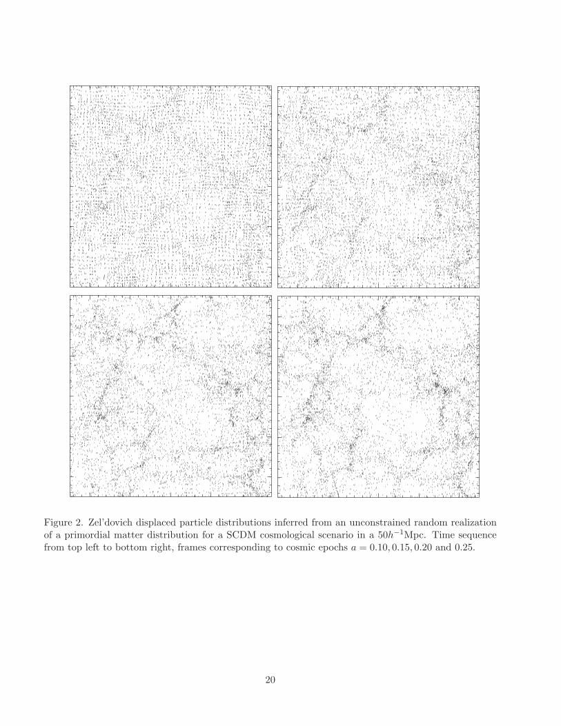
Figure 2. Zel’dovich displaced particle distributions inferred from an unconstrained random realizationof a primordial matter distribution for a SCDM cosmological scenario in a 50h−1Mpc. Time sequencefrom top left to bottom right, frames corresponding to cosmic epochs a = 0.10, 0.15, 0.20 and 0.25.

20

it by the explicit expression for the evolution of the tidal tensor Tij in the linear regime of clustering, inwhich Tij is linearly proportional to the shear σij ,

Tij = −3ΩH2

2Hf(Ω)σij (74)

where f(Ω) ≈ Ω0.6. From this consideration we can straightforwardly appreciate that the Zel’dovichapproximation does not obey the Poisson equation. As a consequence, it does represent an exact ap-proximation in the case of a plane-parallel density disturbance as long as the corresponding particletrajectories have not yet intersected others, but breaks down in the case of two- or three-dimensionalperturbations and in general as soon as the particle tracks have crossed. One well-known implication isthat the Zel’dovich approximation gives incorrect results for spherical infall.

4.2. Higher-Order Lagrangian Approximations

With the Zel’dovich approximation basically concerning the first order solution in Lagrangian perturba-tion theory, various extensions and elaborations were formulated attempting to extend the theory to ahigher order, futhering its range of applicability towards more evolutionary more progressive situations.As can be appreciated from Eqn. (#), the Zel’dovich approximation essentially involves a truncation ofthe set of Lagrangian fluid equations through an implicit choice for Tij , equating it linearly proportionalto σij . This implies a tinkering with the Raychaudhury and shear evolution equations. In the Zel’dovichapproximation one therefore need not integrate the tidal evolution equation, the gravity field on a masselement given by a simple extrapolation of initial conditions.

Pursuing along the same track, Bertschinger & Jain (1994) and Hui & Bertschinger (1996) extendedthis to higher-order schemes, both approximations involving the integration of the exact Raychaud-huri and shear evolution and shifting the approximation to the level of the tidal evolution equation.Bertschinger & Jain (1994) tried to make the very specific assumption of setting the magnetic part ofthe Weyl tensor Hij = 0, thus characterized as the “nonmagnetic” approximation. Subsequent workshowed that this does not adhere to a well-defined or easily recognizable generic situation. Along thesame lines, Hui & Bertschinger (1996) defined another approximate scheme, the “local tidal” approxima-tion. This they showed to followed more accurately the predictions of the homogeneous ellipsoidal modelthan the “nonmagnetic” approximation (Bertschinger & Jain 1996) and the Zel’dovich approximation.Interestingly, while the “nonmagnetic” approximation implied collapse into “spindle” like configurationsas the generic outcome of gravitational collapse, the more accurate “local tidal” approximation appearsto agree with the Zel’dovich approximation in that “planar” geometries are more characteristic.

A range of additional approximate schemes, mostly stemming from different considerations, wereintroduced in a variety of publications. Most of them try to deal with the evolution of high-densityregions after the particle trajectories cross and self-gravity of the resulting matter assemblies assumesa dominating role. Notable examples of such approaches are the adhesion approximation (Kofman,Pogosyan & Shandarin 1990), the frozen flow approximation (Matarrese et al. 1992), the frozen potentialapproximation (Brainerd, Scherrer & Villumsen 1993), the truncated Zel’dovich approximation (Coles,Melott & Shandarin 1993), the smoothed potential approximation (Melott, Sathyaprakash & Sahni1996) and higher order Lagrangian perturbation theory (Melott, Buchert & Weiss 1995). The elegantgeneralization of the Zel’dovich approximation by Giavalisco et al. (1993) will be described later withinthe context of the mixed boundary conditions problem (next section). An extensive and balanced reviewof the various approximation schemes may be found in Sahni & Coles (1995).

4.3. Mixed Boundary Conditions

For pure theoretical purposes, cosmological studies may be restricted to considerations involving pureinitial conditions problems. For a given cosmological and structure formation model the initial densityand velocity field are specified, and its evolution subsequently evolved, either by means of approximate

21

Figure 3. Projected orbits reconstructed by the Fast Action Method implementation of the Least ActionPrinciple procdure. Four different levels of approximation are shown. The black dots represent thefinal (present) positions for each object. The blue lines indicate the trajectories followed by the objectsas a function of time. The top-left frame shows FAM reconstructed orbits with Nf = 1 (Zel’dovichapproximation). Subsequently shown are Nf = 2 (top right), Nf = 3 (lower left) and Nf = 6 (lowerright). From Romano-Dıaz, Branchini & van de Weygaert 2002.

22

schemes or by for instance by means of fully nonlinear N-body computer simulations. The outcomeof such studies are then usually analyzed in terms of a variety of statistical measures. These are thencompared to the outcome of the same tests in the case of the observed world.

Alternatively, we may recognize that in many specific cosmological studies we are dealing with prob-lems of mixed boundary conditions. Part of the large scale structures and velocities in the universe mayhave been measured at the present epoch, while some in the limit of very high redshift (e.g. the CMB).Typically, one seeks to compute the velocity field consistent with an observed density structure at thepresent epoch. Conversely, one may wish to deduce the density from the measured peculiar galaxyvelocities. Evidently, the position and velocities of objects at the present epoch are intimately coupledthrough the initial conditions.

In the linear regime, the problem of mixed boundary conditions is easily solved. However, in the caseof the interesting features in e.g. the cosmic foam the density of galaxies can reach values considerablylarger than unity, even on scales of ∼ 10h−1Mpc. The associated velocities therefore need to be computednonlinearly. As may be obvious from the earlier discussions, the nonlinear computation of gravitationalinstabilities in the case of arbitrary configurations is everything but trivial.

N-body codes are rendered obsolete in such issues involving mixed boundary conditions. Their appli-cation is restricted to initial value problems. A further complication of the nonlinear problem of mixedboundary conditions is the multivalued nature of the solutions. Orbit crossing makes identification of thecorrect orbits difficult, and impossible after virialization has erased the memory of the initial conditions.In practice, one is therefore often restricted to laminar flow in the quasi-linear regime. Perturbationsmay have exceeded unity but orbit crossing has not yet obstructed a one-to-one correspondence be-tween the final and initial positions. Evidently, the Zel’dovich approximation forms a good first-orderapproach towards dealing with such issues. Following this, it was applied to the nonlinear problem ofmixed boundary conditions, tested and calibrated using N-body simulations, by Nusser et al. (1991) andNusser & Dekel (1992).

In terms of the physics of the nonlinear systems, a profound suggestion was forwarded by Peebles(1989, 1990). He noticed that mixed boundary conditions naturally lend themselves to an application ofHamilton’s principle. Given the action S of a system of particles

S =

∫ t0

0Ldt =

∫ t0

0dt∑

i

[1

2mia

2x2i −miφ(xi) ] , (75)

in which L is the Lagrangian for the orbits of particles with masses mi and comoving coordinates xi.The exact equations of motion for the particles can be obtained from stationary variations of the actionS. On the basis of Hamilton’s principel one therefore seeks stationary variations of an action subject tofixed boundary conditions at both the initial and final time. Confining oneself to feasible approximateevaluation in this Least Action Principle approach, one describes the orbits of particles as a linearcombination of suitably chosen universal functions of time with unknown coefficients specific to eachparticle presently located at a position xi,0,

xi(D) = xi,0 +

Nf∑

n=1

qn(D) Ci,n . (76)

In the above formulation we choose to use the linear growth mode D(t) as time variable. The functionsqn(D) form a set of Nf time-dependent basis functions, while Ci,n are a set of free parameters whichare determined from evaluating the stationary variations of the action. The basis functions qn(D) areconstrained by two orbital constraints. To ensure that at the present time the galaxies are located attheir observed positions xi(D = 1) = xi,0 we set the boundary constraint qn(1) = 0. The other boundarycondition concerns the constraint that the peculiar motions at early epochs (D = 0) have to vanish, whichin turn ensures initial homogeneity, i.e. limt→0mia

2xi = 0. The choice of base functions essentiallydetermines the approximation scheme. Originally Peebles (1989, 1990) chose the base functions qn(D) =fn(t) to be polynomials of the expansion factor a(t). For small systems this leads to a tractable problem,

23

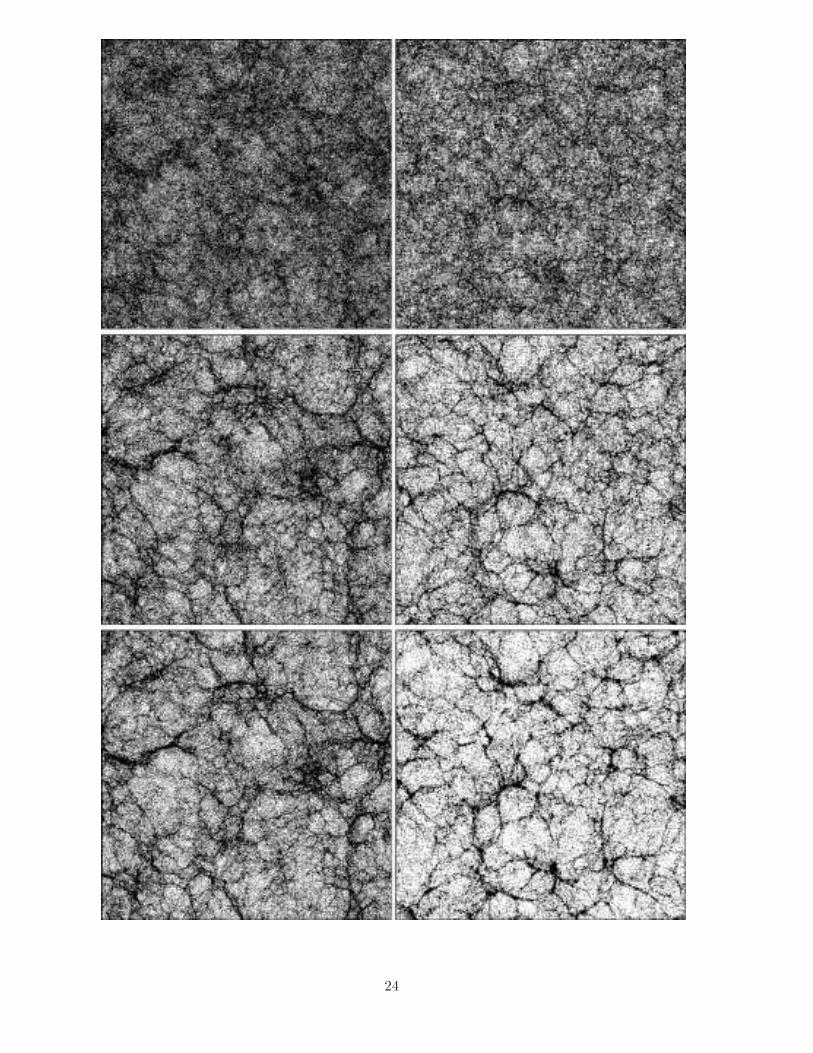
24

Figure 4. Gravitational clustering in scale-free scenarios. Left: n = −2 simulation, at a = 0.2, 0.45, 0.55.Right: n = 1.5 at a = 0.25, 0.63, 1.0. From Smith et al. 2003.

but for larger systems it becomes exceedingly difficult to apply because of confusions between multivaluedsolutions. In an elegant contribution, Giavalisco et al. (1993) merged the Zel’dovich approximation intothe Least Action Principle (LAP) scheme by expanding the formalism into one where the base functionsare higher order polynomials of the linear growth function D(t). In the limit of small displacements,the LAP procedure would then reproduce the Zel’dovich approximation. The higher order terms removethe separability of the temporal and spatial dependence in the Zel’dovich approximation, and allowingarbitrary displacements so that the orbits can be determined to any accuracy. This turned out to yielda rapidly converging scheme, even for highly nonlinear perturbations.

A further improvement of the basic scheme of Giavalisco et al. (1993) was introduced by Nusser &Branchini (2000). They based their computational evaluations of the action on invoking the functionspn(D) ≡ dqn/dD and setting them equal to conveniently defined polynomials of the growth factor D. Inaddition, their Fast Action Method (FAM) involved a computational optimization through the evaluationof the gravitational potential by means of a gravitational TREECODE. This yielded a procedure allowingthe reconstruction of the orbits of 104−105 mass tracing objects back in time and reconstruct the peculiarvelocities of the objects well beyond the linear regime. Its performance can be appreciated from Figure #(from Romano-Dıaz, Branchini & van de Weygaert 2004), in which 4 panels show how the increasinglevels of orbit expansion manage to probe ever deeper into the nonlinear regime. In particular, one caninfer how the Zel’dovich approximation is naturally invoked as the 1st-order step (top left panel).

5. Spherical Model

Analytically tractable idealizations help to understand various aspects of void evolution. In this regard,the spherical model represents the key reference model against which we may assess the evolution of morecomplex configurations. Also, it provides the clearest explanation for the various void characteristicslisted in the main test. And most significantly within the context of this work, it provides the fundamentfrom which our formalism for hierarchical void evolution is developed.

The structure of a spherical void or peak can be treated in terms of mass shells. In the “sphericalmodel” concentric shells remain concentric and are assumed to be perfectly uniform, without any sub-structure. The shells are supposed never to cross until the final singularity, a condition whose validity isdetermined by the initial density profile. The resulting solution of the equation of motion for each shellmay cover the full nonlinear evolution of the perturbation, as long as shell crossing does not occur.

The treatment of the spherical model in a cosmological context has been fully worked out (Gunn &Gott 1973; Lilje & Lahav 1991). As long as the mass shells do not cross, they behave as mini-Friedmannuniverses whose equation of motion assumes exactly the same form as that of an equivalent FRW universewith a modified value of Ωs. The details of the distribution of the mass interior to the shell are of nodirect relevance to the evolution of each individual shell. Instead, the evolution depends on the totalmass contained within the radius of the shell. and the global cosmological background density.

Although quantitative details depend on the cosmological model, a study of the evolution of sphericalperturbations in an Einstein-de Sitter Universe suffices to illustrate all the important physical features.

5.1. Definitions

When a mass shell at some initial time ti starts expanding from a physical radius ri = a(ti)xi, itssubsequent motion is characterized by the expansion factor R(t, ri) of the shell:

r(t, ri) = R(t, ri)ri , (77)

25

26

Figure 5. Similarity in the cosmic structure formation process: the formation of a cluster (from veryhigh resolution simulation by V. Springel) and of a galaxy (T. Quinn), both in ΛCDM scenario.

where r(t, ri) = a(t)x(t, xi) is the physical radius of the shell at time t and x(t, xi) the correspondingcomoving radius. The evolution of the shell is dictated by the cosmological density parameter

Ω(t) =8πGρu(t)

3H2u

(78)

and the mean density contrast within the radius of the shell,

∆(r, t) =3

r3

∫ r

0

[ρ(y, t)

ρu(t)− 1

]y2 dy

=3

r3

∫ r

0δ(y, t) y2 dy , (79)

To determine the evolution of R(t, ri), it is convenient to introduce the parameters ∆ci = ∆c(ti) and αi

where

1 + ∆ci = Ωi [1 + ∆(ti, ri)]

αi =

(vi

Hiri

)2

− 1 . (80)

Here, Ωi = Ω(ti), Hi = H(ti) and vi is the physical velocity (i.e. the sum of the peculiar velocityand Hubble expansion velocity with respect to the void center) of the mass shell at t = ti. The usualassumption of a growing mode perturbation implies that the velocity perturbation vpec,i for a sphericalperturbation, at the initial time ti, is

vpec,i = −Hiri

3f(Ωi)∆(ri, ti) , (81)

and hence,

αi = −2

3f(Ωi)∆(ri, ti) . (82)

In effect, ∆ci is the density contrast of the shell with respect to a critical universe (Ω = 1) at the cosmictime ti, while αi is a measure of the corresponding peculiar velocity (or, rather, the kinetic energy)of the shell. The evolution of a spherical over- or underdensity is entirely and solely determined bythe initial (effective) over- or underdensity within the (initial) radius ri of the shell, ∆ci(ri, ti), and thecorresponding velocity perturbation, vpec,i. Hence, the values of ∆ci and αi determine whether a shellwill stop expanding or not, i.e. whether it is closed, critical or open. The criterion for a closed shell is∆ci > αi, for a critical shell, ∆ci = αi, and ∆ci < αi for an open shell.

Notice that these expressions assume that the initial density fluctuation was negligible, so that theinitial mass m and initial comoving size R are related: m ∝ R3.

5.2. Shell Solutions

The solution for the expansion factor R(t, ri) = R(Θr) of an overdense cq. underdense shell is given bythe parametized expressions

R(Θr) =

12

1 + ∆ci(αi − ∆ci)

(cosh Θr − 1) ∆ci < αi,

12

1 + ∆ci(∆ci − αi)

(1 − cos Θr) ∆ci > αi ,

(83)

27

Figure 6. Spherical Peak 1

28

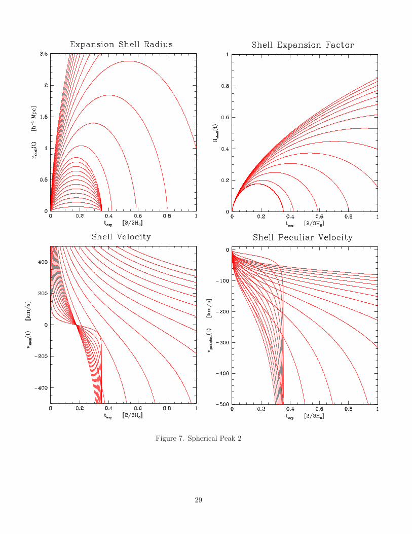
Figure 7. Spherical Peak 2

29

in which the development angle Θr, which paramaterizes all physical quantities relating to the massshell, is related to time t via

t(Θr) =

12

1 + ∆ci

(αi − ∆ci)3/2 (sinh Θr − Θr) ∆ci < αi

12

1 + ∆ci

(∆ci − αi)3/2 (Θr − sinΘr) ∆ci > αi

(84)

while for a critical shell the solution is given by the direct relation

R(Θr) =

3

2Hi(1 + ∆ci)

1/2t

2/3

∆ci = αi . (85)

Notice that the solutions for the evolution of overdense and underdense regions in essence are the same,and are interchangeable by replacing

(sinh Θ − Θ) ⇒ (Θ − sinΘ)

(cosh Θ − 1) ⇒ (1 − cos Θ) . (86)

5.3. Density Evolution

If the initial density contrast of a shell is ∆i(ri), its density contrast ∆(r, t) at any subsequent time t isgiven by

1 + ∆(r, t) =1 + ∆i(ri)

R3

a(t)3

a3i

, (87)

With ∆(r, t) being a relative quantity, comparing the density of the mass shell at radius r at time t withthat of the global cosmic background, the value of ∆(r, t) is a function of the shell’s development angleΘr as well as that of the development angle of the Universe Θu,

Ω =

2coshΘu + 1

Ω < 1,

2cos Θu + 1 Ω > 1.

(88)

The shell’s density contrast may then be obtained from

1 + ∆(r, t) = f(Θr)/f(Θu), (89)

where f(Θ) is the cosmic “density” function:

f(Θ) =

(sinhΘ − Θ)2

(coshΘ − 1)3open ,

2/9 critical ,

(Θ − sinΘ)2

(1 − cos Θ)3closed ,

(90)

This expression is equally valid for the shell (in which case “open” means ∆ci < αi) and the globalbackground Universe (where “open” means Ω < 1).

30

5.4. Shell Velocities

The velocity of expansion or contraction of a spherical shell is given by computing dR/dt, so it can bewritten in terms of Θr and Θu. In particular, the shell’s peculiar velocity with respect to the globalHubble velocity,

vpec(r, t) = v(r, t) −Hu(t)r(t) , (91)

may be inferred from the expression

vpec(r, t) = Hu(t)r(t)

g(Θr)

g(Θu)− 1

, (92)

where Hu(t)r = (a/a)r and the cosmic “velocity” function is

g(Θ) =

sinh Θ (sinhΘ − Θ)

(coshΘ − 1)2open ,

23 critical ,

sinΘ (Θ − sinΘ)

(1 − cosΘ)2closed

(93)

Thus, we may define a Hubble parameter Hs for each individual shell,

Hs(r, t) ≡R

R= Hu(t)

g(Θr)

g(Θu)

. (94)

5.5. Overdensities and collapse when Ω = 1

The previous sections provided explicit expressions for the evolution of a spherical perturbation in FRWbackgrounds with no cosmological constant. To better illustrate our argument, we will now specialize tothe case of an Einstein de-Sitter model. It will prove useful to contrast the spherical evolution with thatpredicted by linear theory. We will use D(z) to denote the linear density perturbation growth factor,normalized so that D(z = 0) = 1. For an Einstein-de Sitter Universe,D(z) = 1/(1 + z). Note that thismakes D ∝ (t/t0)

2/3. Similarly, the growth of velocities in linear theory is given by

vlin(r) = −Hur

3f(Ω)∆(r, t) , (95)

where f(Ω) ≈ Ω0.6 (Peebles 1980). It is a useful exercise to verify that, in its early stages (i.e., smalldevelopment angle), the spherical evolution model does indeed reproduce linear theory.

Consider the evolution of an initially overdense (or, rather, bound) shell. Such a shell will initiallyexpand slightly slower than the background, this expansion gradually slowing to a complete halt, afterwhich it turns around and starts to contract. At turnaround, v(r, t) = 0, so Θr = π, and the density is

1 + ∆(r, tta) = (3π/4)2. (96)

Therefore, at turnaround, the comoving radius of a spherical perturbation has shrunk by a factor of(3π/4)2/3 = 1.771 from what it was initially. Had the perturbation evolved according to linear theory,then turnaround would happen at that redshift when the linear theory prediction ∆lin, reaches the valueδta:

∆lin(zta) = δta = (3/5)(3π/4)2/3 ≈ 1.062. (97)

Full collapse is associated with Θr = 2π. At this time, the linearly extrapolated initial overdensityreaches the threshold value δc,

∆lin(zc) = δc =

(3

5

)(3π

2

)2/3

≈ 1.686 . (98)

31

This makes it straightforward to determine the collapse redshift zcoll of each bound perturbation directlyfrom a given initial density field. In terms of the primordial field linearly extrapolated to the presenttime, ∆lin,0, the collapse redshift zcoll may be directly inferred from

D(zcoll)∆lin,0 = δc . (99)

so

1 + zcoll =∆lin,0

1.686. (100)

Formally, at collapse, the comoving radius is vanishingly small (R(2π) = 0). In reality, the matter in thecollapsing object will virialize as interactions between matter in the shells will exchange energy betwenthe shells and ultimately an equilibrium distribution will be found. Therefore, it is usual to assumethat the final size of a collapsed spherical object is finite and equal to its virial radius. For a perfecttophat density, the object’s final size Rfin is then ≈ 5.622 times smaller than it was initially (Gunn &Gott 1973), i.e.

Rfin/Ri,coll = (18π2)1/3 ≈ 5.622 , (101)

where Ri,coll ≡ Ri(acoll/ai).

5.6. Underdensities and shell-crossing when Ω = 1

Underdense spherical regions evolve differently than their overdense peers. The outward directed peculiaracceleration is directly proportional to the integrated density deficit ∆(r, t) of the void. In the genericcase, the inner shells “feel” a stronger deficit, and thus a stronger outward acceleration, than the outershells.

Once again, to better illustrate our argument, we will now specialize to the case of an Einsteinde-Sitter model. The density deficit evolves as

1 + ∆(r, z) ≈9

2

(sinh Θr − Θr)2

(cosh Θr − 1)3. (102)

In comparison, the corresponding linear initial density deficit ∆lin(z):

∆lin(z) =∆lin,0

1 + z≈ −

3

4

2/3 (sinhΘr − Θr)2/3

5/3. (103)

The (peculiar) velocity with which the void expands into its surroundings is

vpec(r, t) = Hur

3

2

sinhΘr (sinh Θr − Θr)

(cosh Θr − 1)2− 1

. (104)

As a consequence of the differential outward expansion within and around the void, and the accom-panying decrease of the expansion rate with radius r, shells start to accumulate near the boundary of thevoid. The density deficit |∆(r)| of the void decreases as a function of radius r, down to a minimum atthe center. Shells which were initially close to the centre will ultimately catch up with the shells furtheroutside, until they eventually pass them. This marks the event of shell crossing. The correspondinggradual increase of density will then have turned into an infinitely dense ridge. From this moment on-ward the evolution of the void may be described in terms of a self-similar outward moving shell (Sutoet al. 1984; Fillmore & Goldreich 1984; Bertschinger 1985). Strictly speaking, this only occurs for voidswhose density profile is sufficiently steep, since a sufficiently strong differential shell acceleration mustbe generated. This condition is satisfied at the step-function density profile near the edge of a tophatvoid.

32

Figure 8. Spherical Voids

For a tophat void in an Einstein-de Sitter Universe the shells initially just outside the void’s edgepass through a shell crossing stage at a precisely determined value of the mass shell’s development angleΘr = Θsc,

sinhΘsc (sinhΘsc − Θsc)

(cosh Θsc − 1)2=

8

9, so Θsc ≈ 3.53. (105)

At this shell-crossing stage, the average density within the void is

1 + ∆(r, t) = 0.1982 (106)

times that the cosmic background density. This means that the shell has expanded by a factor of(0.1982)−1/3 ≈ 1.7151. In comparison, the underdensity estimated using linear theory at the time ofshell crossing is

∆lin(zsc) = δv = −

(3

4

)2/3 (sinh Θsc − Θsc)2/3

5/3≈ −2.81 . (107)

In terms of the primordial density field, the shell-crossing redshift zsc of a void with (linearly extrapolated)density deficit ∆lin,0 may therefore be directly predicted. For an Einstein-de Sitter Universe it is

1 + zsc =|∆lin,0|

2.8059. (108)

And at shell-crossing, the void has a precisely determined excess Hubble expansion rate:

Hs = (4/3)Hu(tsc), (109)

with Hu = Hu(tsc) the global Hubble expansion factor at tsc.For a spherical underdensity, the instant of shell crossing marks a dynamical phase transition. It is

as significant as the full collapse stage reached by an equivalent overdensity. Also, as with the collapse ofthe overdensity the timescales on which this happens are intimately related to the initial density of theperturbation. The instant of shell crossing is determined by the global density parameter Ωi, the initialdensity deficit ∆i of the shell, and the steepness of the density profile. In turn, this link between theinitial void configuration and the void’s shell crossing transition epoch paves the way towards predictingthe nonlinear evolution of the cosmic void population on the basis of the primordial density field.

33

6. Ellipsoidal Model

Understanding the essence of the phenomenon of the formation of anisotropic patterns in the matterdistribution – walls and filaments – is obtained most readily and lucidly through an assessment of anasymptotic idealization, that of the evolution of collapsing homogeneous ellipsoids. Collapsing ellipsoidstend to slow down their collapse along the longest axis while they evolve far more rapidly along the short-est axis. Starting from a near spherical configuration, the net result is a rapid contraction into a highlyflattened structure as the short axis has fully collapsed. When considering the complete (homogenous)ellipsoid as a “fluid” element, the correspondence with the reasoning above is straightforward.

The bare essence of the driving mechanism behind the formation of cosmic walls and filaments ispossibly best appreciated in terms of the dynamical evolution of homogenous ellipsoidal overdensities. Inparticular, the early work by Icke (1972, 1973) elucidated transparently the crucial characteristics of theirdevelopment and morphology. On the basis of an assessment of the collapse of homogeneous ellipsoidsin an expanding FRW background Universe – following the formalism of Lynden-Bell (1964) and Lin,Mestel & Shu (1965) – he came to the conclusion that flattened and elongated geometries of large scalefeatures in the Universe should be the norm. This description intrinsically involves the self-amplifyingeffect of a collapsing and progressively flattening isolated ellipsoidal overdensity. Quintessential wasIcke’s observation that gravitational instability not only involves the runaway gravitational collapse ofany cosmic overdensity, but that it has the additional basic attribute of inevitably amplifying any slight

initial asphericity during the collapse. In order to appreciate the dynamics behind the process, and beable to assess its action within more complex situations, it is insightful to focus in some detail on theevolution of homogeneous ellipsoids.

6.0.1. Homogeneous Ellipsoidal Model: the Formalism

The ellipsoidal approximation involves an ellipsoidal region with a triaxially symmetric geometry, de-scribed in terms of its principal axes c1, c2 and c3. The matter density in the interior of the ellipsoidhas a constant value of ρell, and the ellipsoid is embedded in a background with a density ρu. While thebasic formalism assumes an isolated ellipsoid, we seek to extend this to a more generic configuration inwhich the ellipsoidal object is subjected to an external tidal field induced by matter fluctuations beyondits immediate neighbourhood. It should be noted that in principle such a configuration is a contrivedone, the existence of an external field implying a contradictio in terminis with respect to the assumptionof a homogeneous background. The intention therefore is to use this as a description reasonably approx-imating and illuminating relevant effects. In the presence of an this external potential contribution, thetotal gravitational potential Φ(tot)(r) in the interior of a homogeneous ellipsoid is given by

Φ(tot)(r) = Φb(r) + Φ(int,ell)(r) + Φ(ext)(r) , (110)

in which (r1, r2, r3) figure as the coordinates in an arbitrary Cartesian coordinate system. In this, wehave decomposed the total potential Φ(tot)(r) into three separate (quadratic) contributions,

• The potential contribution of the homogeneous background with universal density ρu(t),

Φb(r) =2

3πGρu (r21 + r22 + r23) . (111)

• The interior potential Φ(int,ell)(r) of the ellipsoidal entity, superimposed onto the homogeneousbackground,

Φ(int,ell)(r) =1

2

∑

m,n

Φ(int,ell)mn rmrn

=2

3πG(ρell − ρu) (r21 + r22 + r23) +

1

2

∑

m,n

T (int)mn rmrn ,

(112)

34

Figure 9. The evolution of an overdense homogeneous ellipsoid, with initial axis ratio a1 : a2 : a3 =1.0 : 0.9 : 0.9, embedded in an Einstein-de-Sitter background Universe. The two frames show a timesequel of the ellipsoidal configurations attained by the object, starting from a near-spherical shape,initially trailing the global cosmic expansion, and after reaching a maximum expansion turning aroundand proceeding inexorably towards ultimate collapse as a highly elongated ellipsoid. Left: the evolutiondepicted in physical coordinates. Red contours represent the stages of expansion, blue those of thesubsequent collapse after turn-around. Right: the evolution of the same object in comoving coordinates,a monologous procession through ever more compact and more elongated configurations.

35

with T(int)mn the elements of the traceless internal tidal shear tensor,

T (int)mn ≡

∂2Φ(int,ell)

∂rm∂rn−

1

3∇2Φ(int,ell) δmn . (113)

• The externally imposed gravitational potential Φ(ext). We assume that the external tidal fieldnot to vary greatly over the expanse of the ellipsoid, so that we can presume the tidal tensorelements to remain constant within the ellipsoidal region (cf. Dubinski & Carlberg 1991). In

this approximation, the elements T(ext)mn of the external tidal tensor correspond to the quadrupole

components of the external potential field, with the latter being a quadratic function of the (proper)coordinates r = (r1, r2, r3):

Φ(ext)(r) =1

2

∑

m,n

T (ext)mn rmrn . (114)

with the components T(ext)mn of the external tidal shear tensor,

T (ext)mn (t) ≡

∂2Φ(ext)

∂rm∂rn, (115)

which by default, because of its nature, is a traceless tensor. Note that the quadratic form of theexternal potential is a necessary condition for the treatment to remain selfconsistent in terms ofthe ellipsoidal formalism.

As the ellipsoidal formalism does not include any self-consistent external potential, we have to imposeit ourselves in an artificial way, including a specified time evolution of the tidal tensor components (seediscussion in section on external tidal action, eqn. # to #), In essence, we impose an artificial externaltidal field based on the assumption that the background in the immediate vicinity of the ellipsoid remainshomogenous and that the external structures engendering the tidal field are located out at distancessufficiently far away from the ellipsoidal entity. This warrants the validity of the approximation by thequadratic equations, and assures that these external entities themselves are untouched themselves bythe ensuing evolution of the object.

The quadratic expression for the internal ellipsoidal potential contribution Φ(int,ell) can be cast intoa simplified form by choosing a convenient coordinate system in which the coordinate axes coincide withthe principal axes of the ellipsoid. In this case, the expression for the potential of an ellipsoid witheffective density (ρell − ρu) and axes c1, c2 and c3 reduces to (Lyttleton 1953)

Φ(int,ell)(r) = πG (ρell − ρu)∑

m

αmr2m , (116)

where the coefficients αm are determined by the shape of the ellipsoid,

αm = c1c2c3

∫ ∞

0(c2m + λ)−1

3∏

n=1

1√c2n + λ

dλ . (117)

As a consequence of the Poisson equation the αm’s obey the constraint:∑3

m=1 αm = 2. Also, we seethat the components of the internal tidal shear tensor are given by,

T (int)mn = 2πG(ρell − ρu)

(αm −

2

3

)δmn . (118)

It is easy to appreciate that in the case of a spherical perturbation all three αm’s are equal to 2/3,reproducing the well-known fact that in such case the internal tidal tensor contributions need to vanish.

36

From the quadratic nature of the total potential, the acceleration of a mass at a position r inside theellipsoid, −∇Φ(r), is a linear function of r,

d2rm

dt2= −

4π

3Gρurm(t) −

∑

n

Φ(int,ell)mn rn(t) −

∑

n

T (ext)mn rn(t) . (119)

This leads to a linear relation between the location r(t) = (r1(t), r2(t), r3(t)) of a mass element at timet and its initial (proper) position ri = (r1,i, r2,i, r3,i),

rm(t) =∑

k

Rmk(t)rk,i (120)

in which the matrix Rmn(t) is a spatially uniform matrix, solely dependent on time. Notice that theinitial matrix Rmn(t) is a diagonal matrix, Rmn(ti) = Rm(ti)δmn. By combining Eqn. (#) and Eqn.(#), the evolution of the matrix elements Rmk is found to be described by

d2Rmk

dt2= −

4π

3πGRmk −

∑

n

Φ(int,ell)mn Rnk −

∑

n

TmnRnk (121)

This also implies that similar points in concentric ellipsoidal shells behave in the same way, while theellipsoid will remain homogeneous.

To appreciate the ramifications for the shape of an evolving ellipsoidal object, we exclude the torque-ing and angular momentum inducing effects of the external tidal field. To this end, we make thesimplifying assumption of the principal axes of the external tidal tensor to be aligned along the principalaxes of the inertia tensor Iij of the ellipsoid. Of course, in realistic situations we would not expectto find such a perfect alignment between the tidal and the inertia tensors. Yet, there is a significantcorrelation between orientation of tidal field and orientation of the principal axes of a peak/dip in aGaussian random field. In particular, it implies a tendency to align the strongest tidal field componentalong the smallest axis (Van de Weygaert & Bertschinger 1996).

The principal axis alignment implies – when defining the coordinate system by the principal axes

of the ellipsoid – that all off-diagonal (external) tidal tensor elements vanish, T(ext)mn = T

(ext)mm δmn. This

implies∑

n T(ext)mn Rnk = T

(ext)mm Rmk. The resulting equation for the evolution of the matrix elements Rmk

is then described by the second order diffential equation,

d2Rmk

dt2= −2πG

[αmρ

ell + (2

3− αm) ρu

]Rmk − T (ext)

mm Rmk . (122)

Evidently, the coupling between the different components Rmk vanishes. As they are initially equalto zero this implies the non-diagonal elements Rmk(t) to remain so, Rmk(t) = Rm(t)δmn. At timet, a mass element initially at (proper) position ri = (r1,i, r2,i, r3,i) has therefore moved to positionr(t) = (r1(t), r2(t), r3(t)) = (R1(t)r1,i, R2(t)r2,i, R3(t)r3,i), in which the functions Rm(t) evolve accordingto

d2Rm

dt2= −2πG

[αmρ

ell + (2

3− αm) ρu

]Rm − T (ext)

mm Rm . (123)

The evolution of the ellipsoid is thus fully encapsulated in terms of the the functions R1(t), R2(t) andR3(t), which in essence should be seen as scale factors of the principal axes of the ellipsoid,

cm(t) = Rm(t)cm,i . (124)

For any initial configuration of a homogeneous ellipsoid embedded in a FRW background Universe withcurrent cosmic density parameter Ω and Hubble parameter H, specified by its initial characteristics atcosmic expansion factor ai,

• The initial principal axes, (c1, c2, c3).

37

• The initial ellipsoidal density ρelli , in terms of density contrast δi

δi ≡ρell

i − ρui

ρui

, (125)

with respect to the background Universe with initial cosmic density

ρui =3

2ΩH

(aai

)3

(126)

the evolution of the scale factors Rm(t) can be fully recovered once the boundary conditions have beenset, i.e.

• The initial scale factors,Rm(ti) = 1 (127)

for (m = 1, 2, 3).

• The initial velocity perturbation,

vm(ti) = (dRm/dt) rm,i = vHubble,m(ti) + vpec,m(ti)

= Hi Rmrm,i + vpec,m(ti) ,

(128)

for (m = 1, 2, 3), which when choosing to follow the growing mode solution of linear perturbationtheory (Peebles 1980) is given by

vpec,m(ti) =2f(Ωi)

3HiΩigpec,m(ti)

= −1

2Hif(Ωi)

[αm,iδi +

4T(ext)mm,

3Ω0H20

Di

]rm,i .

(129)

In the latter expression, f(Ωi) is the corresponding linear velocity growth factor (Peebles 1980). Theαm,i are the values of the ellipsoidal shape factors αm at expansion factor, which are yielded afterevaluating the integral expression (#) for the specified initial axis ratios. For this expression, we specifiedthe (artificially imposed) time development of the external tidal tensor through a growth factor D(t),

Emm/ΩH2 ∝ D(t), relating the current external tidal field T

(ext)mm, to its initial value.

6.0.2. Homogeneous Ellipsoidal Model: the Approximation

Evidently, we have to be aware of the serious limitations of the ellipsoidal model. It grossly oversimplifiesin disregarding important aspects like the presence of substructure in and the immediate vicinity of peaksand dips in the primordial density field, the sites it typically deals with. Even more serious is its neglectof any external influence, whether the secondary infall or “collision” with surrounding matter or the roleof nonlocal tidal field engendered by the external mass distribution. For overdensities it represents areasonable approximation for moderately evolved features like a Megaparsec (proto)supercluster, but itwill be seriously flawed in the case of highly collapsed objects like galaxies and even clusters of galaxies.Nonethelss, the concept of homogeneous ellipsoids has proven to be particularly useful when seekingto develop approximate yet advanced descriptions of the distribution of virialized cosmological objects(Bond & Myers 1996a,b,c, and Sheth, Mo & Tormen 2001).

Interestingly, in many respects the homogeneous model is a better approximation for underdenseregions than it is for overdense ones. Overdense regions contract into more compact and hence steeper

38

Figure 10. The evolution of an overdense homogeneous ellipsoid, with initial axis ratio a1 : a2 : a3 =1.0 : 0.8 : 0.6, in an Einstein-de-Sitter background Universe. Left: expansion factors for each individualaxis; right: axis ratios a2/a1 and a3/a1. The ellipsoid axes are depicted as red curves. For comparison,in blue, the evolution of an equivalent homogenous spherical overdensity.

density peaks, so that the area in which the ellipsoidal model represents a reasonable approximationwill continuously shrink. On the other hand, while voids expand and get drained, the density fields inthe central region of the (proto)void will flatten out, so that the voids develop into regions of a nearlyuniform density and the region of validity of the approximation grows accordingly. This can be readilyappreciated from the conceptually simpler spherical model approximation. More significant, it was alsodemonstrated in the complex circumstances of voids embedded in a general cosmic density field for a setof N-body structure formation simulations (Van de Weygaert & van Kampen 1993, see Fig. #). A directrepercussion of the flattening out of the voids is the velocity field inside them. With the exception ofthe ridges surrounding them, the quadratic potential approximation will be valid for most of the void’sinterior and therefore be characterized by a velocity field of excess Hubble expansion. The systematicstudy by Van de Weygaert & Van Kampen (1993) indicated how the void velocity fields in general willevolve towards a state in which they become genuine “Superhubble Bubbles” (see section #). Evidently,the ellipsoidal approximation will only be useful for the interior of voids. At the outer fringes the neglectof the role of surrounding material will be rendered invalid, as the sweeping up of matter, the formationand subsequent induced ‘self-interaction’ and the encounter with surrounding structures will becomedomineering effects.

7. N-body simulations

With the exception of a few attempts towards an Eulerian implementation (e.g. Peebles 1987), effortswhich gradually gain more ground with the inclusion of gas-dynamical and radiative processes, compu-tational efforts have concerned N-body computer simulations. By nature, this involves a translation ofthe evolution of a system into a Lagrangian formulation, in which the computer gets instructed to followthe path of each particle into which the initial density field had been broken up. Fully nonlinear N-bodycomputer simulations have produced the most readily visible, and directly appealing and accessible,descriptions of the way into which the gravitational instability process manages to mould the primordialuniverse into rich structural patterns.

Truely giant technological advances over the past decades have provided us with a comprehensive,physically justified and badly needed visual impression of the way into which the mutual influence of thecombined gravitational forces unleashed by the matter perturbations throughout the cosmos works itsway towards the emergence of structure. It has allowed the recognition of some basic mechanisms duringthe full nonlinear evolution of self-gravitating systems. The spatial patterns in the resulting particledistributions, as well as their kinematics and dynamics, provide us with an excellent testbed for testingand comparing quantitatively a large range of viable structure formation scenarios. However, they suffer

39

from a variety of restricting effects, and we should be anxious not to overinterpret and/or overestimatethe results of their performance.

Firstly, they can only go as far as allowed by the physics implemented into them. They will andcannot reveal basic new science to us. The full array of relevant physics, in particular when we get belowscales of clusters of galaxies, is not confined to merely gravitational influences. Radiative processes, acomplex interplay of various hydrodynamic processes, star formation processes, and the full impact ofinvolved feedback interactions should make us realize the limitations of the outcome of the calculations.A large industry of new complex computer codes attempt to deal with at least a selection of theseinfluences. They, however, also illustrate the daunting and possible unsurmountable challenges awaitingus in formulating a fully and uniquely defined scenario of structure formation, incorporating everynecessary aspect of relevant physics.

Even when restricting ourselves to purely gravitational systems, strictly only applicable to scalesat which nongravitational dissipation can be fully discarded as irrelevant, their results should still beconsidered as merely approximate and indicative. Their dynamic range is usually very limited. Thisis true for the feasible spatial resolution, for the attainable mass resolution, as well as for the range oftimescales that can be covered by them. As available computer memory will always restrict these, thefull spatial range of fluctuations – even influential ones – can never be properly represented within agiven cosmic region. A representation of the full primordial power spectrum of density fluctuations isbeyond the grasp of any conceivable piece of equipment. It is therefore important that claims of validityof specific formation scenarios can never be fully justified. In addition, the limited dynamic range willalso restrict the force resolution during the nonlinear evolution, which is particularly cumbersome onthe smallest scales which produce the first nonlinear entities. In addition, we see a rapid increase incomputational expense as we try to improve the resolution. Even though the availability of ultrafastcomputing machinery with ever growing huge memory capacity has expanded the achievements of cos-mological N-body computer simulations to truely dramatic levels, the demands grow along with them,a pace not necessarily followed equally fast by the insights going along with them.

An additional restriction for N-body codes is that they can strictly only be applied to initial valueproblems (see section 3.5.3). For pure theoretical purposes, this does not pose a restriction. For agiven cosmological and structure formation model the initial density and velocity field are specified andsubsequently evolved and analyzed. However, when turning to the observed world, we may recognizethat we are usually dealing with analyzing situations in which most information is available for thepresent epoch. In most cases this involves nonlinear structures for which we are not able to extrapolatein a straightforward and direct fashion towards the initial conditions. Hence we are unable to use N-bodytechniques towards analyzing the implications for the dynamics and evolution of the observed structures.

Possibly the most important limitation of computer calculations may be that the understandingof the dynamics and physics of the simulated systems is not significantly increased. Simulations will

not increase our understanding of dynamics without guidance from analytical approaches, and thereforeanalytical approximations will be absolutely essential for that purpose. Along one direction, these doprovide us with a handle to interpret the outcome of the computer experiments. Equally important,they direct us in defining the best possible computer models and configurations.

Even more important it is to be aware that full understanding involves the formulation of analyticaldescriptions, which should embody our insights into the systematics and regularities of a system, thetrue purpose of scientific inquiry. Analytical descriptions should therefore be the preferred endgoal, thecomputer experiments, along with the ever growing body of available observations, are there to guideand sharpen our insight and intuition.

40