chapter 6 stochastic regressors - home -...
TRANSCRIPT
Chapter 6 Stochastic Regressors• 6.1 Stochastic regressors in non-longitudinal
settings• 6.2 Stochastic regressors in longitudinal settings• 6.3 Longitudinal data models with heterogeneity
terms and sequentially exogenous regressors• 6.4 Multivariate responses• 6.5 Simultaneous equation models with latent
variables• Appendix 6A – Linear projections
6.1 Stochastic regressors in non-longitudinal settings
• 6.1.1 Endogenous stochastic regressors• 6.1.2 Weak and strong exogeneity• 6.1.3 Causal effects• 6.1.4 Instrumental variable estimation
• This section introduces stochastic regressors by focusing on purely cross-sectional and purely time series data.
• It reviews the non-longitudinal setting, to provide a platform for the longitudinal data discussion.
Non-stochastic explanatory variables
• Traditional in the statistics literature• Motivated by designed experiments
– X represents the amount of fertilizer applied to a plot of land.
• However, for survey data, it is natural to think of random regressors. Observational data ????
• On the one hand, the study of stochastic regressors subsumes that of non-stochastic regressors. – With stochastic regressors, we can always adopt the
convention that a stochastic quantity with zero variance is simply a deterministic, or non-stochastic, quantity.
• On the other hand, we may make inferences about population relationships conditional on values of stochastic regressors, essentially treating them as fixed.

Endogenous stochastic regressors• An endogenous variable is one that fails an exogeneity
requirement – more later. • It is customary in economics
– to use the term endogenous to mean a variable that is determined within an economic system whereas
– an exogenous variable is determined outside the system. – Thus, the accepted econometric/statistic usage differs
from the general economic meaning.• If (xi, yi) are i.i.d, then imposing the conditions
E (yi | xi ) = xi′ β and Var (yi | xi ) = σ 2
are sufficient to estimate parameters.• Define εi = yi - xi′ β, and write the first condition as
E (εi | xi ) = 0.• Interpret this to mean that εi and xi are uncorrelated.

Assumptions of the Linear Regression Model with Strictly Exogenous Regressors
Wish to analyze the effect of all of the explanatory variables on the responses. Thus, define X = (x1, …, xn) and require
• SE1. E (yi | X) = xi′ β.• SE2. {x1, …, xn} are stochastic variables.• SE3. Var (yi | X) = σ 2.• SE4. {yi | X} are independent random variables.• SE5. {yi} is normally distributed, conditional on {X}.

Usual Properties Hold• Under SE1-SE4, we retain most of the desirable properties
of our ordinary least square estimators of β. These include: – the unbiasedness and– the Gauss-Markov property of ordinary least square
estimators of β.• If, in addition, SE5 holds, then the usual t and F statistics
have their customary distributions, regardless as to whether or not X is stochastic.
• Define the disturbance term to be εi = yi - xi′ β and – write SE1 as E (εi | X) = 0– is known as strict exogeneity in the econometrics
literature.
Some Alternative Assumptions• Regressors are said to be predetermined if • SE1p. E (εi xi) = E ( (yi - xi′ β) xi) = 0.• The assumption SE1p is weaker than SE1.
– SE1 does not work well with time-series data– SE1p is sufficient for consistent for consistency, not
asymptotic normality.• For asymptotic normality, we require a somewhat stronger
assumption:• SE1m. E ( εi | εi-1, …, ε1, xi , …, x1) = 0 for all i .• When SE1m holds, then {εi} satisfies the requirements for a
martingale difference sequence. • Note that SE1m implies SE1p.

Weak and strong exogeneity• For linear model exogeneity
– We have considered strict exogeneity and predeterminedness.
– Appropriately done in terms of conditional means.– It gives precisely the conditions needed for inference
and is directly testable. • Now we wish to generalize these concepts to assumptions
regarding the entire distribution, not just the mean function.– Although stronger than the conditional mean versions,
these assumptions are directly applicable to nonlinear models.
• We now introduce two new kinds of exogeneity, weak and strong exogeneity.
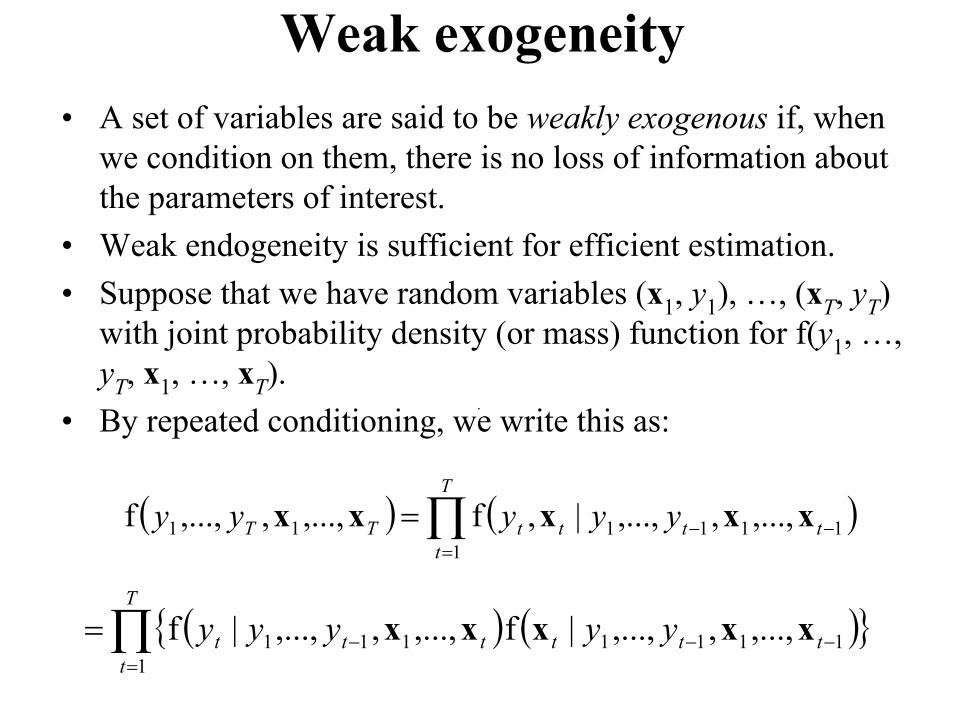
Weak exogeneity• A set of variables are said to be weakly exogenous if, when
we condition on them, there is no loss of information about the parameters of interest.
• Weak endogeneity is sufficient for efficient estimation.• Suppose that we have random variables (x1, y1), …, (xT, yT)
with joint probability density (or mass) function for f(y1, …, yT, x1, …, xT).
• By repeated conditioning, we write this as:
( ) ( )∏=
−−=T
tttttTT yyyyy
1111111 ,...,,,...,|,f,...,,,...,f xxxxx
( ) ( ){ }∏=
−−−=T
ttttttt yyyyy
11111111 ,...,,,...,|f,...,,,...,|f xxxxx
.
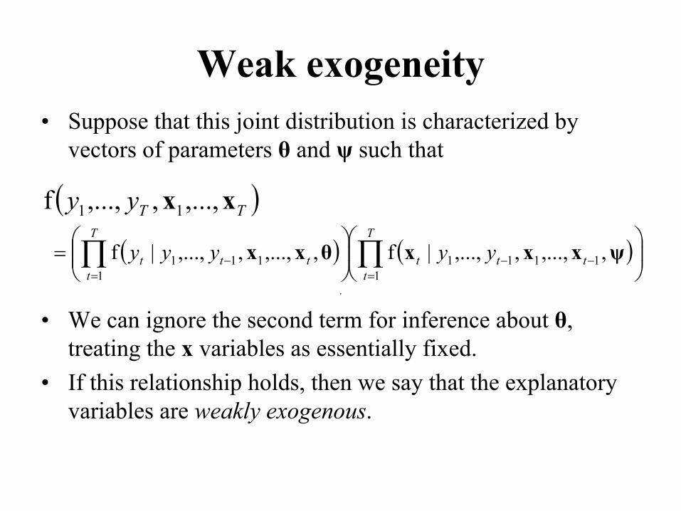
Weak exogeneity• Suppose that this joint distribution is characterized by
vectors of parameters θ and ψ such that
• We can ignore the second term for inference about θ, treating the x variables as essentially fixed.
• If this relationship holds, then we say that the explanatory variables are weakly exogenous.
( )TTyy xx ,...,,,...,f 11
( ) ( )
= ∏∏
=−−
=−
T
tttt
T
tttt yyyyy
11111
1111 ,,...,,,...,|f,,...,,,...,|f ψxxxθxx
.

Strong Exogeneity• Suppose, in addition, that
• that is, conditional on x1, …, xt-1, that the distribution of xtdoes not depend on past values of y, y1, …, yt-1. Then, we say that {y1, …, yt-1} does not Granger-cause xt.
• This condition, together with weak exogeneity, suffices for strong exogeneity.
• This is helpful for prediction purposes.
( ) ( )ψxxxψxxx ,,...,|f,,...,,,...,|f 111111 −−− = ttttt yy

Causal effects • Researchers are interested in causal effects, often more so
than measures of association among variables. • Statistics has contributed to making causal statements
primarily through randomization. – Data that arise from this random assignment mechanism
are known as experimental. – In contrast, most data from the social sciences are
observational, where it is not possible to use random mechanisms to randomly allocate observations according to variables of interest.
• Regression function measures relationships developed through the data gathering mechanism, not necessarily the relationships of interest to researchers.

Structural Models• A structural model is a stochastic model representing a
causal relationship, as opposed to a relationship that simply captures statistical associations.
• A sampling based model is derived from our knowledge of the mechanisms used to gather the data. – The sampling based model directly generates statistics
that can be used to estimate quantities of interest– It is also known as an estimable model.

Causal Statements• Causal statements are based primarily on substantive hypotheses in
which the researcher carefully develops. • Causal inference is theoretically driven. • Causal processes cannot be demonstrated directly from the data; the
data can only present relevant empirical evidence serving as a link in a chain of reasoning about causal mechanisms.
• Longitudinal data are much more useful in establishing causal relationships than (cross-sectional) regression data because, for most disciplines, the “causal” variable must precede the “effect” variables in time.
• Lazarsfeld and Fiske (1938) considered the effect of radio advertising on product sales. – Traditionally, hearing radio advertisements was thought to increase
the likelihood of purchasing a product. – Lazarsfeld and Fiske considered whether those that bought the
product would be more likely to hear the advertisement, thus positing a reverse in the direction of causality.
– They proposed repeatedly interviewing a set of people (the ‘panel’) to clarify the issue.

Instrumental variable estimation • Instrumental variable estimation is a general technique to handle
problems associated with the disconnect between the structural model and a sampling based model.
• To illustrate, consider the linear modelyi = xi′ β + εi ,
yet not all of the regressors are predetermined, E (εi xi) ≠ 0. • Assume there a set of predetermined variables, wi, where
– E (εi wi) = 0 (predetermined)– E (wi wi′) is invertible.
• An instrumental variable estimator of β is bIV = (X΄ PW X)-1 X΄ PW y,
where PW = W (W΄W )-1 W΄ is a projection matrix and W = (w1, …, wn)΄ is the matrix of instrumental variables.
• Within X΄ PW is X΄ W = • this sum of cross-products drives the calculation fo the correlation
between x and w.
∑ ′i iiwx
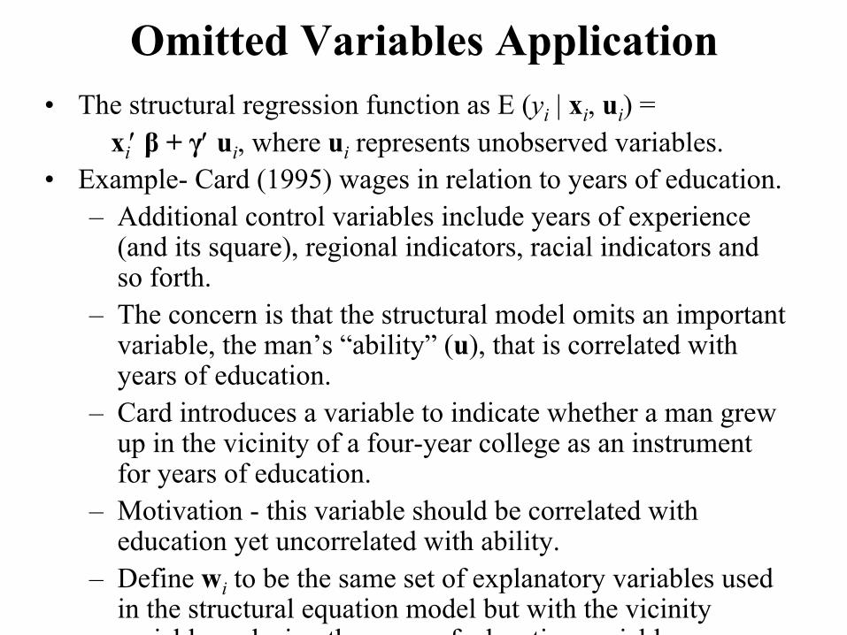
Omitted Variables Application• The structural regression function as E (yi | xi, ui) =
xi′ β + γ′ ui, where ui represents unobserved variables. • Example- Card (1995) wages in relation to years of education.
– Additional control variables include years of experience (and its square), regional indicators, racial indicators and so forth.
– The concern is that the structural model omits an important variable, the man’s “ability” (u), that is correlated with years of education.
– Card introduces a variable to indicate whether a man grew up in the vicinity of a four-year college as an instrument for years of education.
– Motivation - this variable should be correlated with education yet uncorrelated with ability.
– Define wi to be the same set of explanatory variables used in the structural equation model but with the vicinity variable replacing the years of education variable.

Instrumental Variables• Additional applications include:
– Measurement error problems– Endogeneity induced by systems of equations (Section
6.5).• The choice of instruments is the most difficult decision faced
by empirical researchers using instrumental variable estimation.
• Try to choose instruments that are highly correlated with the endogeneous explanatory variables.
• Higher correlation means that the bias as well as standard errorof bIV will be lower.
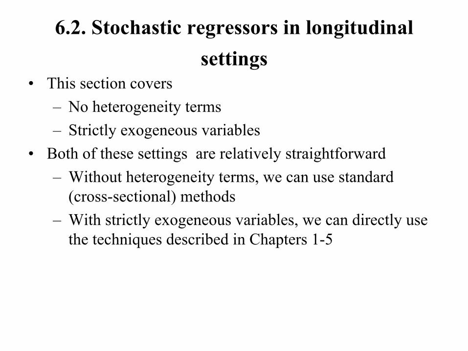
6.2. Stochastic regressors in longitudinal settings
• This section covers– No heterogeneity terms– Strictly exogeneous variables
• Both of these settings are relatively straightforward– Without heterogeneity terms, we can use standard
(cross-sectional) methods– With strictly exogeneous variables, we can directly use
the techniques described in Chapters 1-5
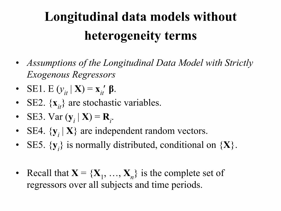
Longitudinal data models without heterogeneity terms
• Assumptions of the Longitudinal Data Model with Strictly Exogenous Regressors
• SE1. E (yit | X) = xit′ β.• SE2. {xit} are stochastic variables.• SE3. Var (yi | X) = Ri.• SE4. {yi | X} are independent random vectors.• SE5. {yi} is normally distributed, conditional on {X}.
• Recall that X = {X1, …, Xn} is the complete set of regressors over all subjects and time periods.

Longitudinal data models without heterogeneity terms
• No heterogeneity terms, but one can incorporate dependence among observations from the same subject with the Rimatrix (such as an autoregressive model or compound symmetry ).
• These strict exogeneity assumptions do not permit lagged dependent variables, a popular approach for incorporating intra-subject relationships among observations. – However, one can weaken this to a pre-determined
condition such as:– SE1p. E (εit xit) = E ( (yit – xit′ β) xit) = 0.
• Without heterogeneity, longitudinal and panel data models have the same endogeneity concerns as the cross-sectional models.

Longitudinal data models with heterogeneity terms and strictly
exogenous regressors• From customary usage or a structural modeling viewpoint,
it is often important to understand the effects of endogenous regressors when a heterogeneity term αi is present in the model.
• We consider the linear mixed effects model of the formyit = zit′ αi + xit′ β + εit
• and its vector versionyi = Zi αi + Xi β + εi .
• Define X* = {X1, Z1, …, Xn, Zn} to be the collection of all observed explanatory variables and
• α = (α1′, …, αn′)′ to be the collection of all subject-specific terms.
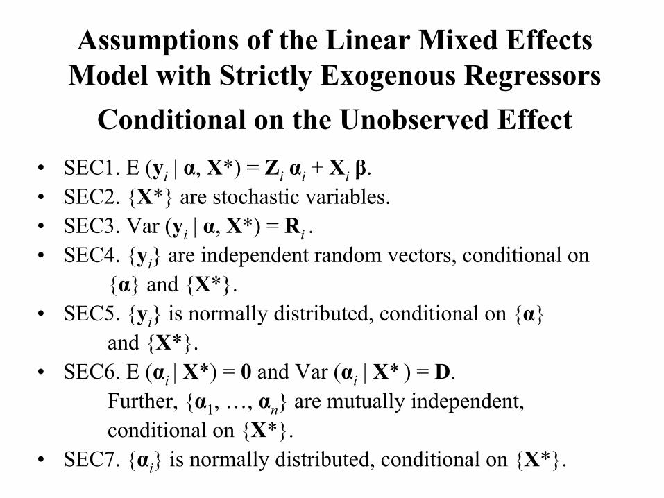
Assumptions of the Linear Mixed Effects Model with Strictly Exogenous Regressors
Conditional on the Unobserved Effect• SEC1. E (yi | α, X*) = Zi αi + Xi β.• SEC2. {X*} are stochastic variables.• SEC3. Var (yi | α, X*) = Ri .• SEC4. {yi} are independent random vectors, conditional on
{α} and {X*}.• SEC5. {yi} is normally distributed, conditional on {α}
and {X*}.• SEC6. E (αi | X*) = 0 and Var (αi | X* ) = D.
Further, {α1, …, αn} are mutually independent, conditional on {X*}.
• SEC7. {αi} is normally distributed, conditional on {X*}.

Observables Representation of the Linear Mixed Effects Model with Strictly Exogenous
Regressors Conditional on the Unobserved Effect
• SE1. E (yi | X* ) = Xi β.• SE2. {X*} are stochastic variables.• SE3a. Var (yi | X*) = Zi D Zi′ + Ri.• SE4. {yi} are independent random vectors,
conditional on {X*}.• SE5. {yi} is normally distributed,
conditional on {X*}.

Strictly Exogenous Regressors Conditional on the Unobserved Effect
• These assumptions are stronger than strict exogeneity.• For example, note that E (yi | α, X*) = Zi αi + Xi β and
E (αi | X*) = 0 together imply thatE (yi | X*) = E (E ( yi | α, X*) | X*)
= E (Zi αi + Xi β | X*) = Xi β .• That is, we require strict exogeneity of the
disturbances (E (εi | X*) = 0) and• that the unobserved effects (α) are uncorrelated with
the disturbance terms (E (εi α′) = 0).
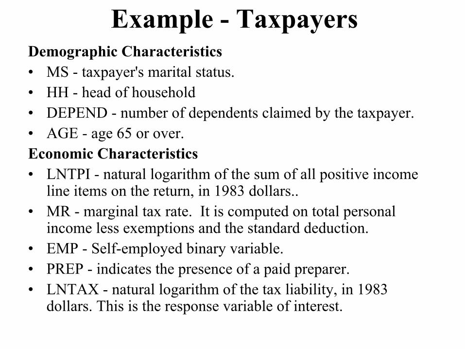
Example - TaxpayersDemographic Characteristics• MS - taxpayer's marital status. • HH - head of household • DEPEND - number of dependents claimed by the taxpayer.• AGE - age 65 or over.Economic Characteristics• LNTPI - natural logarithm of the sum of all positive income
line items on the return, in 1983 dollars..• MR - marginal tax rate. It is computed on total personal
income less exemptions and the standard deduction.• EMP - Self-employed binary variable.• PREP - indicates the presence of a paid preparer.• LNTAX - natural logarithm of the tax liability, in 1983
dollars. This is the response variable of interest.

Example - Taxpayers• Because the data was gathered using a random sampling mechanism,
we can interpret the regressors as stochastic.• Demographics, and probably EMP, can be safely argued as strictly
exogenous.• LNTAXt should not affect LNTPIt, because LNTPI is the sum of
positive income items, not deductions.• Tax preparer variable (PREP)
– it may be reasonable to assume that the tax preparer variable ispredetermined, although not strictly exogenous.
– That is, we may be willing to assume that this year’s tax liability does not affect our decision to use a tax preparer because we do not know the tax liability prior to this choice, making the variablepredetermined.
– However, it seems plausible that the prior year’s tax liability will affect our decision to retain a tax preparer, thus failing the strict exogeneity test.
Taxpayer Model -With heterogeneity terms• Consider the error components model
– We interpret the heterogeneity terms to be unobserved subject-specific (taxpayer) characteristics, such as “ability,”that would influence the expected tax liability.
– One needs to argue that the disturbances, representing “unexpected” tax liabilities, are uncorrelated with the unobserved effects.
• Moreover, Assumption SEC6 employs the condition that the unobserved effects are uncorrelated with the observed regressor variables. – One may be concerned that individuals with high earnings
potential who have historically high levels of tax liability (relative to their control variables) may be more likely to use a tax preparer, thus violating this assumption.
Fixed effects estimation• If one is concerned with Assumption SEC6, then a solution
may be fixed effects estimation (even when we believe in a random effects model formulation).
• Intuitively, this is because the fixed effects estimation procedures “sweep out” the heterogeneity terms– they do not rely on the assumption that they are
uncorrelated with observed regressors.• Some analysts prefer to test the assumption of correlation
between unobserved and observed effects by examining the difference between these two estimators – “Hausman test”Section 7.2.

6.3 Longitudinal data models with heterogeneity
terms and sequentially exogenous regressors
• The assumption of strict exogeneity, even when conditioning on unobserved heterogeneity terms, is limiting.– Strict exogeneity rules out current values of the response (yit)
feeding back and influencing future values of the explanatory variables (such as xi,t+1).
• An alternative assumption introduced by Chamberlain (1992) allows for this feedback.
• We say that the regressors are sequentially exogenous conditional on the unobserved effects if
E ( εit | αi, xi1, …, xit ) = 0. or (in the error components model)
E ( yit | αi, xi1, …, xit ) = αi + xit΄ β for all i, t.
• After controlling for αi and xit, no past values of regressorsaffect the expected value of yit.

Lagged dependent variable model• This formulation allows us to consider lagged dependent
variables as regressorsyit = αi + γ yi,t-1 + xit′ β + εit ,
• This is sequentially exogenous conditional on the unobserved effects– To see this, use the set of regressors oit = (1, yi,t-1, xit′)′
and E (εit | αi, yi,1, …, yi,t-1, xi,1, …, xi,t) = 0. – The explanatory variable yi,t-1 is not strictly exogenous
so that the Section 6.2.2 discussion does not apply.

Estimation difficulties of lagged dependent variable model
• Estimation of the lagged dependent variable model is difficult because the parameter γ appears in both the mean and variance structure.
Cov (yit, yi,t-1) = Cov (αi + γ yi,t-1 + xit′ β + εit , yi,t-1) = Cov (αi, yi,t-1) + γ Var (yi,t-1).
andE yit = γ E yi,t-1 + xit′ β = γ (γ E yi,t-2 + xi,t-1′ β ) + xit′ β
= … = (xit′ + γ xi,t-1′ +…+ γ t-2 xi,2′)β + γ t-1 E yi,1 .• Thus, E yit clearly depends on γ. • Moreover, special estimation techniques are required.

First differencing technique• First differencing proves to be a suitable device for
handling certain types of endogenous regressors.• Taking first differences of the lagged dependent variable
model yieldsyit - yi,t-1 = γ ( yi,t-1 - yi,t-2) + εit - εi,t-1 ,
eliminating the heterogeneity term. • Ordinary least squares estimation using first differences
(without an intercept term) yields an unbiased and consistent estimator of γ.
• First differencing can also fail - see the “feedback”example.

Example – Feedback• Consider the error components yit = αi + xit′ β + εit where
{εit} are i.i.d. • Suppose that the current regressors are influenced by the
“feedback” from the prior period’s disturbance through the relation xit = xi,t-1 + υi εi,t-1, where {υi} is an i.i.d.
• Taking differences of the model, we have∆ yit = yit - yi,t-1 = ∆ xit′ β + ∆εit
where ∆εit = εit - εi,t-1 and ∆xit = xit - xi,t-1 = υi εi,t-1.
• The ordinary least squares estimator of β are asymptotically biased.– Due to the correlation between ∆xit and ∆εit.
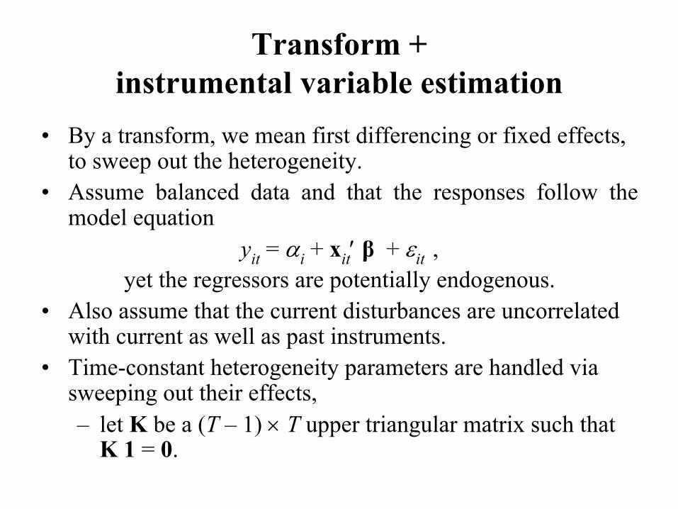
Transform +instrumental variable estimation
• By a transform, we mean first differencing or fixed effects, to sweep out the heterogeneity.
• Assume balanced data and that the responses follow the model equation
yit = αi + xit′ β + εit ,yet the regressors are potentially endogenous.
• Also assume that the current disturbances are uncorrelated with current as well as past instruments.
• Time-constant heterogeneity parameters are handled via sweeping out their effects, – let K be a (T – 1) × T upper triangular matrix such that
K 1 = 0.

• Thus, the transformed system isK yi = K Xi′ β + K εi ,
• Could use first differences
• So that
−−
−−
=
110000011000
000110000011
L
L
MMMOMMM
L
L
FDK
−
−−
=
−−
−−
=
−−
1
23
12
1
2
1
110000011000
000110000011
TTT
T
FD
yy
yyyy
yy
yy
MM
L
L
MMMOMMM
L
L
yK

• Arrellano and Bover (1995) recommend
• Defining εi,FOD = KFOD εi, the tth row is
• These are known as “forward orthogonal deviations.” They are used in time series – have slightly better properties.
−
−−
−−
−−
−−
−−
−−
−−
−−
−−
−−
−=
11000021
211000
21
21
21
2110
11
11
11
11
111
21
1diag
L
L
MMMOMMM
L
L
L TTTT
TTTTT
TT
FODK
( )
++
−−
+−−
= + TitiitFODit tTtTtT
,1,, ...11
εεεε
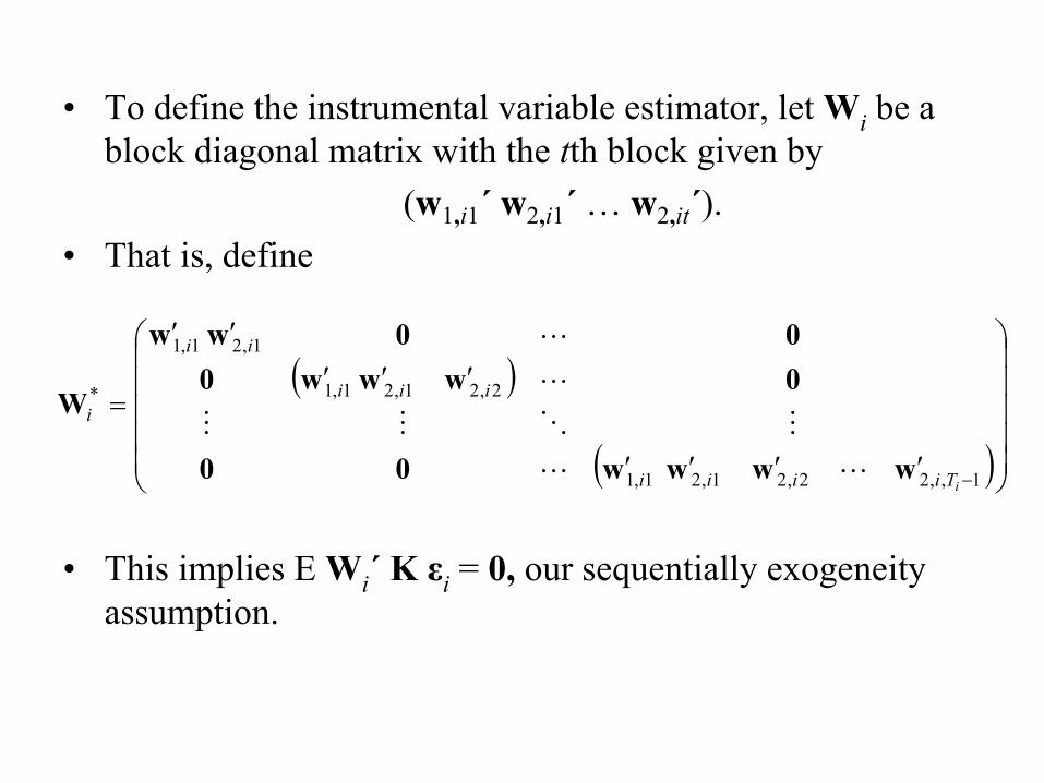
• To define the instrumental variable estimator, let Wi be a block diagonal matrix with the tth block given by
(w1,i1´ w2,i1´ … w2,it´). • That is, define
• This implies E Wi´ K εi = 0, our sequentially exogeneity assumption.
( )
( )
′′′′
′′′′′
=
−1,,22,21,21,1
2,21,21,1
1,21,1
*
iTiiii
iii
ii
i
wwww00
0www000ww
W
LL
MOMM
L
L
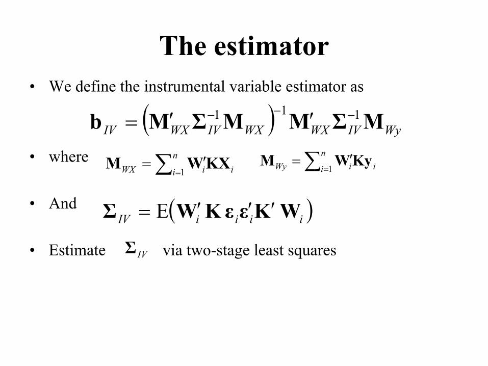
The estimator• We define the instrumental variable estimator as
• where
• And
• Estimate via two-stage least squares
( ) WyIVWXWXIVWXIV MΣMMΣMb 111 −−− ′′=
∑ =′=
n
i iiWX 1KXWM ∑=
′=n
i iiWy 1KyWM
( )iiiiIV WKεεKWΣ ′′′= E
IVΣ

Feedback Example• Recall the relation xit = xi,t-1 + υi εi,t-1, .• A natural set of instruments is to choose wit = xit. • For simplicity, use the first difference transform.• With these choices, the tth block of E Wi´ KFD εi is
• so the sequentially exogeneity assumption is satisfied.
( )
=−
+
0
0
x
xMM titi
it
i
,1,
1
E εε

Taxpayer Example• We suggested that a heterogeneity term may be due to an
individual’s earning potential – this may be correlated with the variable that indicates
use of a professional tax preparer. • Moreover, there was concern that tax liabilities from one
year may influence the choice in subsequent tax year’s choice of whether or not to use a professional tax preparer.
• If this is the case, then the instrumental variable estimator provides protection against this sequential endogeneity concern.

6.4 Multivariate responses• 6.4.1 Multivariate regressions• 6.4.2 Seemingly unrelated regressions• 6.4.3 Simultaneous equations models• 6.4.4 Systems of equations with error
components

6.5 Simultaneous-Equations Models with Latent Variables
• 6.5.1 Cross-Sectional Models• 6.5.2 Longitudinal Data Applications