Chapter 6 Multiple Regression

Timothy Hanson

Department of Statistics, University of South Carolina

Stat 704: Data Analysis I

1 / 33

6.1 Multiple regression models

We now add more predictors, linearly, to the model. For examplelet’s add one more to the simple linear regression model:

Yi = β0 + β1xi1 + β2xi2 + εi ,

with the usual E (εi ) = 0. For any Y in this population withpredictors (x1, x2) we have

µ(x1, x2) = E (Y ) = β0 + β1x1 + β2x2.

The triple (x1, x2, µ(x1, x2)) = (x1, x2, β0 + β1x1 + β2x2) describesa plane in R3 (p. 215).

2 / 33

Multiple regression models

Generally, for k = p − 1 predictors x1, . . . , xk our model is

Yi = β0 + β1xi1 + β2xi2 + · · ·+ βkxik + εi , (6.7)

with mean

E (Yi ) = β0 + β1xi1 + β2xi2 + · · ·+ βkxik . (6.8)

β0 is mean response when all predictors equal zero (if thismakes sense).

βj is the change in mean response when xj is increased by oneunit but the remaining predictors are held constant.

We will assume normal errors:

ε1, . . . , εniid∼ N(0, σ2).

3 / 33

Dwayne Portrait Studio data (Section 6.9)

Dwayne Portrait Studio is doing a sales analysis based on datafrom 21 cities.

Y = sales (thousands of dollars) for a city

x1 = number of people 16 years or younger (thousands)

x2 = per capita disposable income (thousands of dollars)

Assume the linear model is appropriate. One way to checkmarginal relationships is through a scatterplot matrix. However,these are not infallible.

For these data, is β0 interpretable?

β2 is the change in the mean response for a thousand-dollarincrease in disposable income, holding “number of people under 16years old” constant.

4 / 33

SAS code

data studio;

input people16 income sales @@;

label people16=’Number 16 and under (thousands)’

income =’Per capita disposable income ($1000)’

sales =’Sales ($1000$)’;

datalines;

68.5 16.7 174.4 45.2 16.8 164.4 91.3 18.2 244.2 47.8 16.3 154.6

46.9 17.3 181.6 66.1 18.2 207.5 49.5 15.9 152.8 52.0 17.2 163.2

48.9 16.6 145.4 38.4 16.0 137.2 87.9 18.3 241.9 72.8 17.1 191.1

88.4 17.4 232.0 42.9 15.8 145.3 52.5 17.8 161.1 85.7 18.4 209.7

41.3 16.5 146.4 51.7 16.3 144.0 89.6 18.1 232.6 82.7 19.1 224.1

52.3 16.0 166.5

;

proc sgscatter; matrix people16 income sales / diagonal=(histogram kernel); run;

options nocenter;

proc reg data=studio;

model sales=people16 income / clb; * clb gives 95% CI for betas;

run; * alpha=0.9 for 90% CI, etc.;

5 / 33

SAS output

The REG Procedure

Analysis of Variance

Sum of Mean

Source DF Squares Square F Value Pr > F

Model 2 24015 12008 99.10 <.0001

Error 18 2180.92741 121.16263

Corrected Total 20 26196

Root MSE 11.00739 R-Square 0.9167

Dependent Mean 181.90476 Adj R-Sq 0.9075

Coeff Var 6.05118

Parameter Estimates

Parameter Standard

Variable Label DF Estimate Error t Value Pr > |t| 95% Confidence Limits

Intercept Intercept 1 -68.85707 60.01695 -1.15 0.2663 -194.94801 57.23387

people16 Number 16 and 1 1.45456 0.21178 6.87 <.0001 1.00962 1.89950

under (thousands)

income Per capita disposable 1 9.36550 4.06396 2.30 0.0333 0.82744 17.90356

income ($1000)

6 / 33

Scatterplot matrix

7 / 33

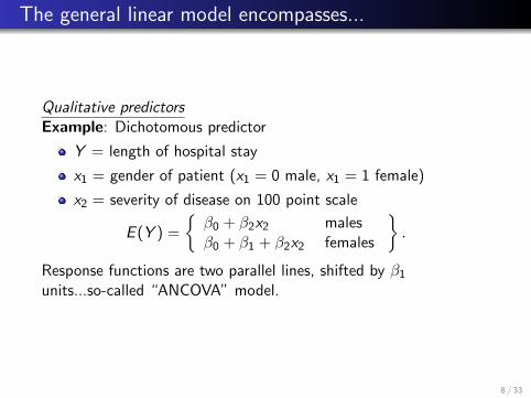
The general linear model encompasses...

Qualitative predictorsExample: Dichotomous predictor

Y = length of hospital stay

x1 = gender of patient (x1 = 0 male, x1 = 1 female)

x2 = severity of disease on 100 point scale

E (Y ) =

{β0 + β2x2 malesβ0 + β1 + β2x2 females

}.

Response functions are two parallel lines, shifted by β1

units...so-called “ANCOVA” model.

8 / 33

The general linear model encompasses...

Polynomial regressionOften appropriate for curvilinear relationships between responseand predictor.Example:

Y = β0 + β1x1 + β2x21 + ε.

Letting x2 = x21 this is in the form of the general linear model.

Transformed responseExample:

log Y = β0 + β1x1 + β2x2 + β3x3 + ε.

Let Y ∗ = log(Y ) and get general linear model.

9 / 33

The general linear model encompasses...

Interaction effectsExample:

Y = β0 + β1x1 + β2x2 + β3x1x2 + ε.

Let x3 = x1x2 and get general linear model.

Key: All of these models are linear in the coefficients, the βj terms.An example of a model that is not in general linear model form isexponential growth:

Y = β0 exp(β1x) + ε.

10 / 33

6.2 General linear model in matrix terms

Let Y =

Y1

Y2...

Yn

be the response vector.

Let X =

1 x11 x12 · · · x1k

1 x21 x22 · · · x2k...

......

. . ....

1 xn1 xn2 · · · xnk

be the design matrix

containing the predictor variables. The first column is aplace-holder for the intercept term. What does each columnrepresent? What does each row represent?

11 / 33

General linear model in matrix terms

Let β =

β0

β1...βk

be the unkown vector of regression coefficients.

Let ε =

ε1

ε2...εn

be the unobserved error vector.

12 / 33

General linear model in matrix terms

The general linear model is written in matrix terms asY1

Y2...

Yn

︸ ︷︷ ︸

n×1

=

1 x11 x12 · · · x1k

1 x21 x22 · · · x2k...

......

. . ....

1 xn1 xn2 · · · xnk

︸ ︷︷ ︸

n×p

β0

β1...βk

︸ ︷︷ ︸

p×1

+

ε1

ε2...εn

︸ ︷︷ ︸

n×1

,

where p = k + 1, or succinctly as

Y = Xβ + ε.

13 / 33

General linear model in matrix terms

Minimal assumptions about the random error vector ε are

E (ε) = 0 and cov(ε) = Inσ2,

where In is the n × n identity matrix (zero except for 1’s along thediagonal).

In general, we will go farther and assume

ε ∼ Nn(0, Inσ2).

This allows use to construct t and F tests, obtain confidenceintervals, etc.

Writing the model like this saves a lot of time and space as we goalong.

14 / 33

6.3 Fitting the model

Estimating β = (β0, β1, . . . , βk)′

Recall least-squares method: minimize

Q(β) =n∑

i=1

[Yi − (β0 + β1xi1 + · · ·βkxik)]2,

as a function of β. Vector calculus can show that the least-squaresestimates are

b =

b0

b1...

bk

= (X′X)−1X′Y,

typically found using a computer package. Note: there is a typo inthe book (equation (6.25) p. 223).

15 / 33

6.4 Fitted values & residuals

The fitted values are in the vector

Y =

Y1

Y2...

Yn

= Xb = [X(X′X)−1X′]︸ ︷︷ ︸projection matrix

Y = HY. (6.30)

The residuals are in the vector

e =

e1

e2...

en

= Y − Y = Y − Xb = [In − X(X′X)−1X′]︸ ︷︷ ︸projection matrix

Y. (6.31)

16 / 33

Hat matrix & Dwayne Studios

H = X(X′X)−1X′ is called the “hat matrix.” We’ll use it shortlywhen we talk about diagnostics. Note also that e = (I−H)Y.

Back to Dwayne Portrait Studio data. From SAS,

b =

b0

b1

b2

=

−68.8571.4559.366

,so the fitted regression line is

Y = −68.857 + 1.455x1 + 9.366x2.

17 / 33

Interpretation

Interpretation of b1: We estimate that for 1000 personincrease in persons 16 and under, mean sales increase by$1,455 (1.455 thousand dollars) holding per capita disposableincome constant.

Interpretation of b2: We estimate that for each $1000increase in per capita disposable income, mean sales increaseby $9,366, holding the number of people under 16 constant.

18 / 33

6.5 Analysis of variance

Again, in multiple regression we can decompose the total sum ofsquares into the SSR and SSE pieces. The table is now

Source SS df MS E(MS)

Regression SSR=∑n

i=1(Yi − Y )2 p − 1 SSRp−1

σ2 + QF

Error SSE=∑n

i=1(Yi − Y )2 n − p SSEn−p

σ2

Total SSTO=∑n

i=1(Yi − Y )2 n − 1

where p = k + 1.Here, QF stands for “quadratic form” and is given by

QF = 12

k∑j=1

k∑s=1

βjβs

n∑i=1

(xij − xj)(xis − xs) ≥ 0.

Note that QF= 0⇔ β1 = β2 = · · · = βk = 0.

19 / 33

Overall F-test for a regression relationship (p. 226)

In multiple regression, our F-test based on F ∗ = MSRMSE tests

whether the entire set of predictors x1, . . . , xk explains a significantamount of the variation in Y .

If MSR ≈ MSE , there’s no evidence that any of the predictors areuseful. If MSR >> MSE , then some or all of them are useful.

Formally, the F-test tests H0 : β1 = β2 = · · · = βk = 0 versus Ha :at least one of these is not zero. If F ∗ > Fp−1,n−p(1− α), wereject H0 and conclude that something is going on, there is somerelationship between or more of the x1, . . . , xk and Y . SASprovides a p-value for this test.

20 / 33

R2 is how much variability soaked up by model

The coefficient of multiple deterimation is

R2 =SSR

SSTO= 1− SSE

SSTO(6.40)

measures the proportion of sample variation in Y explained by itslinear relationship with the predictors x1, . . . , xk . As before,0 ≤ R2 ≤ 1.

When we add a predictor to the model R2 can only increase.

The adjusted R2

R2a = 1− SSE/(n − p)

SSTO/(n − 1)(6.42)

accounts for the number of predictors in the model. It maydecrease when we add useless predictors to the model.

21 / 33

Dwayne Studios, ANOVA table, R2, & R2a

Analysis of Variance

Sum of Mean

Source DF Squares Square F Value Pr > F

Model 2 24015 12008 99.10 <.0001

Error 18 2180.92741 121.16263

Corrected Total 20 26196

Root MSE 11.00739 R-Square 0.9167

Dependent Mean 181.90476 Adj R-Sq 0.9075

Coeff Var 6.05118

We reject H0 : β1 = β2 = 0 at any reasonable significance level α.About 92% of the total variability in the data is explained by thelinear regression model.

22 / 33

Inference about individual regression parameters

The overall F-test concerns the entire set of predictors x1, . . . , xk .

If the F-test is significant (if we reject H0), we will want todetermine which of the individual predictors contribute significantlyto the model.

We will talk about this shortly, but the main methods are forwardselection, backwards elimination, stepwise procedures, Cp, and R2

a .

Aside: There are also fancy new methods including LASSO,LARS, etc. These are used when there’s lots of predictors, e.g.p = 500 or p = 20, 000.

23 / 33

Mean and covariance matrix of a vector

Recall: If Y is a random vector, then its expected value is also avector

E (Y) =

E (Y1)E (Y2)

...E (Yn)

.The random vector Y also has a covariance matrix

cov(Y) =

cov(Y1,Y1) cov(Y1,Y2) · · · cov(Y1,Yn)cov(Y2,Y1) cov(Y2,Y2) · · · cov(Y2,Yn)

......

. . ....

cov(Yn,Y1) cov(Yn,Y2) · · · cov(Yn,Yn)

.

24 / 33

Multivariate normal

An aside: the multivariate normal density is given by

f (y) = |2πΣ|−1/2 exp{−0.5(y − µ)′Σ−1(y − µ)},

where y ∈ Rd . We write

Y ∼ Nd(µ,Σ).

Then E (Y) = µ and cov(Y) = Σ.

For the general linear model,

Y ∼ Nn(Xβ, σ2In).

25 / 33

Error vector

Note that along the diagonal of cov(Y), cov(Yi ,Yi ) = var(Yi ).

For the general linear model,

E (ε) = 0 =

00...0

,

cov(ε) = σ2In =

σ2 0 · · · 00 σ2 · · · 0...

.... . .

...0 0 · · · σ2

.

26 / 33

6.6 Inference for β

cov(Y) = cov( Xβ︸︷︷︸constant

+ ε︸︷︷︸random

) = cov(ε) = Inσ2.

Fact: If A is a constant matrix, a is a constant vector, and Y isany random vector, then

E (AY + a) = AE (Y) + a,

cov(AY + a) = Acov(Y)A′.

27 / 33

Back to the general linear model

For Y = HY,

E (Y) = HE (Y) = HXβ = X(X′X)−1X′Xβ = Xβ.

cov(Y) = Hcov(Y)H′ = σ2H,

since HH′ = H (property of a projection matrix).For e = (In −H)Y,

E (e) = (In −H)E (Y) = (In −H)Xβ = Xβ −HXβ = 0,

as HX = X (projection matrix again).

cov(e) = (In −H)cov(Y)(In −H)′ = σ2(In −H).

(Guess why...)

28 / 33

Mean and variance of b (p. 227)

Finally, b = (X′X)−1X′Y is unbiased

E (b) = (X′X)−1X′E (Y) = (X′X)−1X′Xβ = β,

and has covariance matrix

cov(b) = (X′X)−1X′cov(Y)[(X′X)−1X′]′

= σ2(X′X)−1X′[(X′X)−1X′]′

= σ2(X′X)−1X′X(X′X)−1

= σ2(X′X)−1.

Presto!b ∼ Np(β, σ2(X′X)−1).

29 / 33

Table of regression effects (p. 228)

From the previous slide, the jth estimated coefficient βj ,

var(bj) = σ2cjj ,

where cjj is the jth diagonal element of (X′X)−1. Estimate thestandard deviation of bj by its standard error se(bj) =

√MSEcjj

yieldingbj − βjse(bj)

∼ tn−p (6.49)

Note: SAS gives each se(bj) as well as bj , t∗j = bj/se(bj), and ap-value for testing each H0 : βj = 0.

30 / 33

Dwayne output

Parameter Estimates

Parameter Standard

Variable Label DF Estimate Error t Value Pr > |t| 95% Confidence Limits

Intercept Intercept 1 -68.85707 60.01695 -1.15 0.2663 -194.94801 57.23387

people16 Number 16 and 1 1.45456 0.21178 6.87 <.0001 1.00962 1.89950

under (thousands)

income Per capita disposable 1 9.36550 4.06396 2.30 0.0333 0.82744 17.90356

income ($1000)

We reject H0 : β1 = 0 at the α = 0.01 level and β2 = 0 at theα = 0.05 level.

31 / 33

Individual tests of H0 : βj = 0

Note: A test of H0 : βj = 0 versus Ha : βj 6= 0 – available in thetable of regression coefficients – is a test of whether predictor xj isnecessary in a model with the other remaining predictors included.For the Studio Data:

The SAS summary gives us F ∗ = MSR/MSE = 99.10 withassociated p-value < 0.0001 (it is actually 2× 10−10!). Westrongly reject (at any reasonable α) H0 : β1 = β2 = 0.

95% CI’s are (1.01, 1.90) for β1 and (0.83, 17.90) for β2.

For example, we are 95% confident that mean sales increasesby $1010 to $1900 for every 1000 increase in kids 16 andunder, holding income constant.

For H0 : β1 = 0 we get p < 0.0001; for H0 : β2 = 0 we getp = 0.03. Are people under 16, x1, and income, x2, importantin the model?

32 / 33

Optional output

Model statement model sales=people16 income / covb

corrb;

gives cov(b) and corr(b)

Covariance of Estimates

Variable Label Intercept people16 income

Intercept Intercept 3602.0346743 8.7459395806 -241.4229923

people16 Number 16 and under (thousands) 8.7459395806 0.0448515096 -0.672442604

income Per capita disposable income ($1000) -241.4229923 -0.672442604 16.515755794

Correlation of Estimates

Variable Label Intercept people16 income

Intercept Intercept 1.0000 0.6881 -0.9898

people16 Number 16 and under (thousands) 0.6881 1.0000 -0.7813

income Per capita disposable income ($1000) -0.9898 -0.7813 1.0000

These are not typically used except for more “unusual” analyses;e.g. inference for β1/β2.

33 / 33