CHAPTER 6REFLECTOR ANTENNAS

Helmut E. SchrankGary E. EvansDaniel Davis

Electronic Systems GroupWestinghouse Electric Corporation

6.1 INTRODUCTION

Role of the Antenna. The basic role of the radar antenna is to provide atransducer between the free-space propagation and the guided-wave propagation ofelectromagnetic waves. The specific function of the antenna during transmission isto concentrate the radiated energy into a shaped directive beam which illuminatesthe targets in a desired direction. During reception the antenna collects the energycontained in the reflected target echo signals and delivers it to the receiver. Thusthe radar antenna is used to fulfill reciprocal but related roles during its transmitand receive modes. In both of these modes or roles, its primary purpose is toaccurately determine the angular direction of the target. For this purpose, a highlydirective (narrow) beam width is needed, not only to achieve angular accuracy butalso to resolve targets close to one another. This important feature of a radarantenna is expressed quantitatively in terms not only of the beamwidth but also oftransmit gain and effective receiving aperture. These latter two parameters areproportional to one another and are directly related to the detection range andangular accuracy. Many radars are designed to operate at microwave frequencies,where narrow beamwidths can be achieved with antennas of moderate physical size.

The above functional description of radar antennas implies that a single an-tenna is used for both transmitting and receiving. Although this holds true formost radar systems, there are exceptions: some monostatic radars use separateantennas for the two functions; and, of course, bistatic radars must, by definition,have separate transmit and receive antennas. In this chapter, emphasis will be onthe more commonly used single antenna and, in particular, on the widely usedreflector antennas. Phased array antennas are covered in Chap. 7.

Beam Scanning and Target Tracking. Because radar antennas typically havedirective beams, coverage of wide angular regions requires that the narrowbeam be scanned rapidly and repeatedly over that region to assure detection oftargets wherever they may appear. This describes the search or surveillancefunction of a radar. Some radar systems are designed to follow a target once ithas been detected, and this tracking function requires a specially designedantenna different from a surveillance radar antenna. In some radar systems,

particularly airborne radars, the antenna is designed to perform both searchand track functions.

Height Finding. Most surveillance radars are two-dimensional (2D),measuring only range and azimuth coordinates of targets. In early radarsystems, separate height finding antennas with mechanical rocking motion inelevation were used to determine the third coordinate, namely, elevation angle,from which the height of an airborne target could be computed. More recentdesigns of three-dimensional (3D) radars use a single antenna to measure allthree coordinates: for example, an antenna forming a number of stacked beamsin elevation in the receive mode and a single broad-coverage elevation beam inthe transmit mode. The beams are all equally narrow in azimuth, but thevertically stacked receive beams allow measuring echo amplitudes in twoadjacent overlapping beams to determine the elevation angle of the target.

Classification of Antennas. Radar antennas can be classified into two broadcategories, optical antennas and array antennas. The optical category, as thename implies, comprises antennas based on optical principles and includes twosubgroups, namely, reflector antennas and lens antennas. Reflector antennasare still widely used for radar, whereas lens antennas, although still used insome communication and electronic warfare (EW) applications, are no longerused in modern radar systems. For that reason and to reduce the length of thischapter, lens antennas will not be discussed in detail in this edition of thehandbook. However, references on lens antennas from the first edition will bekept in the list at the end of the chapter.

6.2 BASICPRINCIPLESANDPARAMETERS

This section briefly reviews basic antenna principles with emphasis on definitionsof terms useful to a radar system designer. In order to select the best type ofantenna for a radar system, the system designer should have a clear understand-ing of the basic performance features of the wide variety of antenna types fromwhich he or she must choose.1 This includes the choice between reflector anten-nas, covered in this chapter, and phased arrays, covered in Chap. 7. Another al-ternative is a reflector fed by a phased array.

Although the emphasis in this chapter is on reflectors, many of the basic prin-ciples discussed in this section apply to all antennas. The three basic parametersthat must be considered for any antenna are:

• Gain (and effective aperture)• Radiation pattern (including beamwidth and sidelobes)• Impedance (voltage-standing-wave ratio, or VSWR)

Other basic considerations are reciprocity and polarization, which will be brieflydiscussed in this section.

Reciprocity. Most radar systems employ a single antenna for both trans-mitting and receiving, and most such antennas are reciprocal devices, whichmeans that their performance parameters (gain, pattern, impedance) areidentical for the two functions. This reciprocity principle2 allows the antenna tobe considered either as a transmitting or as a receiving device, whichever is

more convenient for the particular discussion. It also allows the antenna to betested in either role (Sec. 6.10).

Examples of nonreciprocal radar antennas are phased arrays using nonreciprocalferrite components, active arrays with amplifiers in the transmit/receive (TfR) modules,and height finding antennas for 3D (range, azimuth, and elevation) radars. The last-named, typified by the AN/TPS-433 radar, uses several overlapping beams stacked inelevation for receiving with a broad elevation beam for transmitting. All beams areequally narrow in the azimuth direction. These nonreciprocal antennas must be testedseparately for their transmitting and receiving properties.

Gain, Directivity, and Effective Aperture. The ability of an antenna toconcentrate energy in a narrow angular region (a directive beam) is describedin terms of antenna gain. Two different but related definitions of antenna gainare directive gain and power gain. The former is usually called directivity,while the latter is often called gain. It is important that the distinction betweenthe two be clearly understood.

Directivity (directive gain) is defined as the maximum radiation intensity(watts per steradian) relative to the average intensity, that is,

_ maximum radiation intensity _ maximum power per steradianD average radiation intensity total power radiatedMir

This can also be expressed in terms of the maximum radiated-power density (wattsper square meter) at a far-field distance R relative to the average density at that samedistance:

_ maximum power density _ pmaxD ~ total power radiated/4-ir R2 ~ P/4ir R2

Thus the definition of directivity is simply how much stronger the actual maxi-mum power density is than it would be if the radiated power were distributedisotropically. Note that this definition does not involve any dissipative losses inthe antenna but only the concentration of radiated power.

Gain (power gain) does involve antenna losses and is defined in terms ofpower accepted by the antenna at its input port P0 rather than radiated power PThus gain is given by

_ maximum power density _ /?max

total power accepted/4ir R2 /V4ir ^2

For realistic (nonideal) antennas, the power radiated Pt is equal to the power ac-cepted P0 times the radiation efficiency factor TQ of the antenna:

Pt = Vo (6.4)

As an example, if a typical antenna has 1.0 dB dissipative losses, T] = 0.79, and itwill radiate 79 percent of its input power. The rest, (1 - TI) or 21 percent, is con-verted into heat. For reflector antennas, most losses occur in the transmissionline leading to the feed and can be made less than 1 dB.

By comparing Eqs. (6.2) and (6.3) with (6.4), the relation between gain anddirectivity is simply

G = T]G0 (6.5)

Thus antenna gain is always less than directivity except for ideal lossless anten-nas, in which case TJ = 1.0 and G = G0.

Approximate Directivity—Beamwidth Relations. An approximate but usefulrelationship between directivity and antenna beamwidths (see Sec. 2.3) is

40,000GD ^ ̂ - (6.6)

^az^el

where Baz and Z?e, are the principal-plane azimuth and elevation half-powerbeamwidths (in degrees), respectively. This relationship is equivalent to a 1° by 1°pencil beam having a directivity of 46 dB. From this basic combination, the ap-proximate directivities of other antennas can be quickly derived: for example, a1° by 2° beam corresponds to a directivity of 43 dB because doubling onebeamwidth corresponds to a 3 dB reduction in directivity. Similarly, a 2° by 2°beam has 40 dB, a 1° by 10° beam has 36 dB directivity, and so forth. Eachbeamwidth change is translated into decibels, and the directivity is adjusted ac-cordingly. This relation does not apply to shaped (e.g., cosecant-squared) beams.

Effective Aperture. The aperture of an antenna is its physical area projectedon a plane perpendicular to the main-beam direction. The concept of effectiveaperture is useful when considering the antenna in its receiving mode. For anideal (lossless), uniformly illuminated aperture of area A operating at a wave-length X, the directive gain is given by

G0 = 4-TrA/X2 (6.7)

This represents the maximum available gain from an aperture A and implies aperfectly flat phase distribution as well as uniform amplitude.

Typical antennas are not uniformly illuminated but have a tapered illumination(maximum in the center of the aperture and less toward the edges) in order toreduce the sidelobes of the pattern. In this case, the directive gain is less thanthat given by Eq. (6.7):

GD = 4TrA6A2 (6.8)

where Ae is the effective aperture or capture area of the antenna, less than thephysical aperture A by a factor pa usually called the aperture efficiency.

Ae = paA (6.9)

This aperture efficiency would better be called aperture effectiveness becauseit does not involve RF power turned into heat; i.e., it is not a dissipative effectbut only a measure of how effectively a given aperture is utilized. An antennawith an aperture efficiency of, say, 50 percent (pa = 0.5) has a gain 3 dB belowthe uniformly illuminated aperture gain but does not dissipate half the power in-volved. The effective aperture represents a smaller, uniformly illuminated aper-ture having the same gain as that of the actual, nonuniformly illuminated aper-ture. It is the area which, when multiplied by the incident power density P19 givesthe power received by the antenna:

Pr = PtAe (6.10)

Radiation Patterns. The distribution of electromagnetic energy in three-dimensional angular space, when plotted on a relative (normalized) basis, is calledthe antenna radiation pattern. This distribution can be plotted in various ways,e.g., polar or rectangular, voltage intensity or power density, or power per unitsolid angle (radiation intensity). Figure 6.1 shows a typical radiation pattern for acircular-aperture antenna plotted isometrically in terms of the logarithmic powerdensity (vertical dimension in decibels) versus the azimuth and elevation angles inrectangular coordinates. The main lobe (or main beam) of the pattern is a pencilbeam (circular cross section) surrounded by minor lobes, commonly referred to assidelobes. The angular scales have their origins at the peak of the main lobe,which is generally the electrical reference axis of the antenna.

This axis may or may not coincide with the mechanical axis of the antenna,i.e., the axis of symmetry, sometimes called the boresight axis. If the two do notcoincide, which usually happens unintentionally, the angular difference is re-ferred to as a boresight error and must be accounted for in the measurement oftarget directions.

Figure 6. Ia shows the three-dimensional nature of all antenna patterns, whichrequire extensive data to plot in this form. This same data can also be plotted inthe form of constant-power-level contours, as shown in Fig. 6.1c. These contoursare the intersections of a series of horizontal planes through the 3D pattern atvarious levels and can be quite useful in revealing the distribution of power inangular space.

More frequently, however, 2D plots are sufficient and more convenient tomeasure and plot. For example, if the intersection of the 3D pattern of Fig. 6.1awith a vertical plane through the peak of the beam and the zero azimuth angle istaken, a 2D slice or "cut" of the pattern results, as shown in Fig. 6. Ib. This iscalled the principal-plane elevation pattern. A similar cut by a vertical plane or

(o )

FIG. 6.1 Typical pencil-beam pattern, (a) Three-dimensional cartesian plot of complete pattern.

ELEVATION (DEGREES)(b)

AZIMUTH ANGLE( C )

FIG. 6.1 (Continued) (b) Principal-plane elevation pattern, (c) Contours of constant intensity(isophotes). (Courtesy of D. D, Howard, Naval Research Laboratory.)

ELEV

ATION

ANG

LE

db

thogonal to the first one, i.e., containing the peak and the 0° elevation angle, re-sults in the so-called azimuth pattern, also a principal-plane cut because it con-tains the peak of the beam as well as one of the angular coordinate axes.

These principal planes are sometimes called cardinal planes. All other verticalplanes through the beam peak are called inter cardinal planes. Sometimes patterncuts in the ±45° intercardinal planes are measured and plotted, but most often itis sufficient to plot only the azimuth and elevation patterns to describe the pat-tern performance of an antenna. In other words, it is sufficient (and much lesscostly) to sample the 3D pattern with two planar cuts containing the beam axis.

The terms azimuth and elevation imply earth-based reference coordinates,which may not always be applicable, particularly to an airborne or space-based(satellite) system. A more generic pair of principal planes for antennas in generalare the so-called E and H plane of a linearly polarized antenna. Here the E-planepattern is a principal plane containing the direction of the electric (E-field) vectorof the radiation from the antenna, and the H plane is orthogonal to it, thereforecontaining the magnetic (//-field) vector direction. These two principal planes canbe independent of earth-oriented directions such as azimuth and elevation andare widely used.

It should be noted that sampling 3D antenna patterns is not limited to planarcuts as described above. Sometimes it is meaningful and convenient (from ameasuring-technique viewpoint) to take conical cuts, i.e., the intersections of the3D pattern with cones of various angular widths centered on the electrical (or me-chanical) axis of the antenna.

The typical 2D pattern shown in Fig. 6. Ib is plotted in rectangular coordi-nates, with the vertical axis in decibels. This is by far the most widely used formof plotting patterns because it provides a wide dynamic range of pattern levelswith good visibility of the pattern details. However, other forms of plotting-pattern data are also used, as illustrated in Fig. 6.2. This shows four forms ofplotting the same sin x/x pattern, including (a) a polar plot of relative voltage (in-tensity), (b) a rectangular plot of voltage, (c) a rectangular plot of relative power(density), and (d) a rectangular plot of logarithmic power (in decibels). The linearvoltage and power scales in a, b, and c leave much to be desired in showinglower-level pattern details, while d provides good "visibility" of the entire pat-tern. Of course, polar patterns can also be plotted by using decibels in the radialdimension, but lower-level details are compressed near the center of the patternchart and visibility is very poor. Figure 6.2 shows the reason why rectangular-decibel pattern plots are most often preferred.

Beamwidth. One of the main features of an antenna pattern is the beamwidthof the main lobe, i.e., its angular extent. However, since the main beam is a con-tinuous function, its width varies from the peak to the nulls (or minima). Themost frequently expressed width is the half-power beamwidth (HPBW), whichoccurs at the 0.707-relative-voltage level in Fig. 6.2a and b, at the 0.5-relative-power level in c, and at the 3 dB level in d. Sometimes other beamwidths arespecified or measured, such as the one-tenth power (10 dB) beamwidth, or thewidth between nulls, but unless otherwise stated the simple term beamwidth im-plies the half-power (3 dB) width. This half-power width is also usually a measureof the resolution of an antenna, so that two identical targets at the same range aresaid to be resolved in angle if separated by the half-power beamwidth.

The beamwidth of an antenna depends on the size of the antenna aperture aswell as on the amplitude and phase distribution across the aperture. For a givendistribution, the beamwidth (in a particular planar cut) is inversely proportionalto the size of the aperture (in that plane) expressed in wavelengths. That is, thehalf-power beamwidth is given by

HPBW = K/(D/\) = KX/D (6.11)

where D is the aperture dimension, X is the free-space wavelength, and K is aproportionality constant known as the beamwidth factor. Each amplitude distri-bution (assuming a linear phase distribution) has a corresponding beamwidth fac-tor, expressed either in radians or in degrees.

DEGREES DEGREES(c) W

FIG. 6.2 Various representations of the same sin xlx pattern.

POLA

R-RE

LATI

VE

AMPL

ITUD

ERE

LATI

VE P

OWER

RELA

TIVE

AMPL

ITUD

EDE

CIBE

LS R

ELAT

IVE

TO P

EAK

DEGREES(b)(a)

Sidelobes. The lobe structure of the antenna radiation pattern outside themajor-lobe (main-beam) region usually consists of a large number of minor lobes,of which those adjacent to the main beam are sidelobes. However, it is commonusage to refer to all minor lobes as sidelobes, in which case the adjacent lobes arecalled first sidelobes. The minor lobe approximately 180° from the main lobe iscalled the backlobe.

Sidelobes can be a source of problems for a radar system. In the transmitmode they represent wasted radiated power illuminating directions other than thedesired main-beam direction, and in the receive mode they permit energy fromundesired directions to enter the system. For example, a radar for detecting low-flying aircraft targets can receive strong ground echoes (clutter) through thesidelobes which mask the weaker echoes coming from low radar cross-sectiontargets through the main beam. Also, unintentional interfering signals fromfriendly sources (electromagnetic interference, or EMI) and/or intentional inter-ference from unfriendly sources (jammers) can enter through the minor lobes. Itis therefore often (but not always) desirable to design radar antennas withsidelobes as low as possible (consistent with other considerations) to minimizesuch problems. (NOTE: There are systems in which the lowest possible sidelobesare not desirable; for example, to minimize main-beam clutter or jamming, it maybe better to tolerate higher sidelobes in order to achieve a narrower main-beamnull width).

To achieve low sidelobes, antennas must be designed with special tapered am-plitude distributions across their apertures. For a required antenna gain thismeans that a larger antenna aperture is needed. Conversely, for a given size ofantenna, lower sidelobes mean less gain and a correspondingly broaderbeam width. The optimum compromise (tradeoff) between sidelobes, gain, andbeamwidth is an important consideration for choosing or designing radar anten-nas. Figure 7.23 of Chap. 7 shows these tradeoff relations for the optimum Tayloramplitude distribution4'5 being widely used for sidelobe suppression in radar an-tennas. One set of curves is for rectangular (linear) apertures; the other, for cir-cular Taylor distributions.

The sidelobe levels of an antenna pattern can be specified or described in sev-eral ways. The most common expression is the relative sidelobe level, defined asthe peak level of the highest sidelobe relative to the peak level of the main beam.For example, a " — 30 dB sidelobe level" means that the peak of the highestsidelobe has an intensity (radiated power density) one one-thousandth (10 ~3 or-30 dB) that of the peak of the main beam. Sidelobe levels can also be quantifiedin terms of their absolute level relative to isotropic. In the above example, if theantenna gain were 35 dB, the absolute level of the -30 dB relative sidelobe is + 5dBi, i.e., 5 dB above isotropic. For some radar systems, the peak levels of indi-vidual sidelobes are not as important as the average level of all the sidelobes.This is particularly true for airborne "down-look" radars like the Airborne Warn-ing and Control System, or AWACS (E-3A), which require very low (ultralow)average sidelobe levels in order to suppress ground clutter. The average level is apower average (sometimes referred to as the rms level} formed by integrating thepower in all minor lobes outside the main lobe and expressing it in decibels rel-ative to isotropic (dBi). For example, if 90 percent of the power radiated is in themain beam, 10 percent (or 0.1) is in all the sidelobes: this corresponds to an av-erage sidelobe level of -10 dBi. If the main beam contains 99 percent of the ra-diated power, the average sidelobe level is 0.01, or -20 dBi, etc. Ultralow aver-

age sidelobe levels, defined as better than -20 dBi, have been achieved withcareful design and manufacturing processes.

One other way to describe sidelobe levels (not often used but sometimesmeaningful) is by the median level', this is the level such that half of the angularspace has sidelobe levels above it and the other half has them below that level.

Polarization. The direction of polarization of an antenna is defined as the di-rection of the electric-field (E-field) vector. Many existing radar antennas are lin-early polarized, usually either vertically or horizontally; although these designa-tions imply an earth reference, they are quite common even for airborne orsatellite antennas.

Some radars use circular polarization in order to detect aircraftlike targets inrain. In that case, the direction of the E field varies with time at any fixed obser-vation point, tracing a circular locus once per RF cycle in a fixed plane normal tothe direction of propagation. Two senses of circular polarization (CP) are possi-ble, right-hand (RHCP) and left-hand (LHCP). For RHCP, the electric vector ap-pears to rotate in a clockwise direction when viewed as a wave receding from theobservation point. LHCP corresponds to counterclockwise rotation. These defi-nitions of RHCP and LHCP can be illustrated with hands, by pointing the thumbin the direction of propagation and curling the fingers in the apparent direction ofE-vector rotation. By reciprocity, an antenna designed to radiate a particular po-larization will also receive the same polarization.

The most general polarization is elliptical polarization (EP), which can bethought of as imperfect CP such that the E field traces an ellipse instead of a cir-cle. A clear discussion of polarizations can be found in Kraus.6'7

Another increasingly important consideration for radar antennas is not onlywhat polarization they radiate (and receive) but how pure their polarization is.For example, a well-designed vertical-polarization antenna may also radiate smallamounts of the orthogonal horizontal polarization in some directions (usually offthe main-beam axis). Similarly, an antenna designed for RHCP many also radiatesome LHCP, which is mathematically orthogonal to RHCP. The desired polar-ization is referred to as the main polarization (COPOL), while the undesired or-thogonal polarization is called cross polarization (CROSSPOL). Polarization pu-rity is important in the sidelobe regions as well as in the main-beam region. Someantennas with low COPOL sidelobes may, if not properly designed, have higherCROSSPOL sidelobes, which could cause clutter or jamming problems. A well-designed antenna will have CROSSPOL components at least 20 dB below theCOPOL in the main-beam region, and 5 to 10 dB below in the sidelobe regions.Reflecting surfaces near an antenna, such as aircraft wings or a ship superstruc-ture, can affect the polarization purity of the antenna, and their effects should bechecked.

6.3 TYPESOFANTENNAS

Reflector antennas are built in a wide variety of shapes with a corresponding va-riety of feed systems to illuminate the surface, each suited to its particular appli-cation. Figure 6.3 illustrates the most common of these, which are described insome detail in the following subsections. The paraboloid in Fig. 6.3a collimatesradiation from a feed at the focus into a pencil beam, providing high gain andminimum beamwidth. The parabolic cylinder in Fig. 6.3>b performs this

(«) (f) (g)FIG. 6.3 Common reflector antenna types, (a) Paraboloid, (b) Parabolic cylinder, (c) Shaped, (c/)Stacked beam, (e) Monopulse. (/) Cassegrain. (g) Lens.

collimation in one plane but allows the use of a linear array in the other plane,thereby allowing flexibility in the shaping or steering of the beam in that plane.An alternative method of shaping the beam in one plane is shown in Fig. 6.3c, inwhich the surface itself is no longer a paraboloid. This is a simpler construction,but since only the phase of the wave across the aperture is changed, there is lesscontrol over the beam shape than in the parabolic cylinder, whose linear arraymay be adjusted in amplitude as well.

Very often the radar designer needs multiple beams to provide coverage or todetermine angle. Figure 6.3d shows that multiple feed locations produce a set ofsecondary beams at distinct angles. The two limitations on adding feeds are thatthey become defocused as they necessarily move away from the focal point andthat they increasingly block the aperture. An especially common multiple-beamdesign is the monopulse antenna of Fig. 6.3e, used for angle determination on asingle pulse, as the name implies. In this instance the second beam is normally adifference beam with its null at the peak of the first beam.

Multiple-reflector systems, typified by the Cassegrain antenna of Fig. 6.3/, of-fer one more degree of flexibility by shaping the primary beam and allowing thefeed system to be conveniently located behind the main reflector. The symmet-rical arrangement shown has significant blockage, but offset arrangements canreadily be envisioned to accomplish more sophisticated goals.

Lenses (Fig. 6.3g) are not as popular as they once were, largely becausephased arrays are providing many functions that lenses once fulfilled. Primarilythey avoid blockage, which can become prohibitive in reflectors with extensivefeed systems. A very wide assortment of lens types has been studied.8"13

In modern antenna design, combinations and variations of these basic typesare widespread, with the goal of minimizing loss and sidelobes while providingthe specified beam shapes and locations.

(a) (b) (c) (d)

SUM

DIFFERENCE

(a) (b)

FIG. 6.4 Geometrical representation of a paraboloidal reflector, (a) Geometry, (b) Opera-tion.

Paraboloidal Reflector Antennas. The theory and design of paraboloidalreflector antennas are extensively discussed in the literature.2"4-14'15 The basicgeometry is that of Fig. 6Aa, which assumes a parabolic conducting reflectorsurface of focal length / with a feed at the focus F. It can be shown fromgeometrical optics considerations that a spherical wave emerging from F andincident on the reflector is transformed after reflection into a plane wavetraveling in the positive z direction (Fig. 6Ab).

The two coordinate systems that are useful in analysis are shown in Fig. 6Aa.In rectangular coordinates (jc, y, z), the equation of the paraboloidal surface witha vertex at the origin (O, O, O) is

z = (*2 + y2)/4f (6.12)

In spherical coordinates (p, t|/, £) with the feed at the origin, the equation of thesurface becomes

P = /sec2 I (6.13)

This coordinate system is useful for designing the pattern of the feed. For exam-ple, the angle subtended by the edge of the reflector at the feed can be found from

^otany = £>/4/ (6.14)

The aperture angle 2i|;0 is plotted as a function of flD in Fig. 6.5. Reflectors withthe longer focal lengths, which are flattest and introduce the least distortion ofpolarization and of off-axis beams, require the narrowest primary beams andtherefore the largest feeds. For example, the size of a horn to feed a reflector offlD = 1.0 is approximately 4 times that of a feed for a reflector of f/D = 0.25.Most reflectors are chosen to have a focal length between 0.25 and 0.5 times thediameter.

PARABOLICREFLECTION

VERTEX

PLANEWAVEFRONT

BEAMAXIS

FOCUS

f/DFIG. 6.5 Subtended angle of the edge of a paraboloidal reflector.

When a feed is designed to illuminate a reflector with a particular taper, thedistance p to the surface must be accounted for, since the power density in thespherical wave falls off as 1/p2. Thus the level at the edge of the reflector will belower than at the center by the product of the feed pattern and this "spacetaper." The latter is given in decibels as

(4//Z))2

Space taper (dB) = 20 log (6 15)1 + (4//D)2

Equation (6.15) is graphed in Fig. 6.6, showing a significant contribution at thesmaller focal lengths. In low-sidelobe applications this amplitude variation maybe used in conjunction with the feed pattern to achieve a specific shaping to theskirts of the distribution across the aperture.

Although this reflector is commonly illustrated as round with a central feedpoint, a variety of reflector outlines are in use, as shown in Fig. 6.7. Often, the

0 (D

EGRE

ES)

(d) (e) (f)FIG. 6.7 Paraboloidal reflector outlines, (a) Round, (b) Oblong, (c) Offset feed, (d) Mi-tered corner, (e) Square corner. (/) Stepped corner.

azimuth and elevation beam width requirements are quite different, requiring the44orange-peel," or oblong, type of reflector of Fig. 6.1b.

As sidelobe levels are reduced and feed blockage becomes intolerable, offsetfeeds (Fig. 6.7c) become necessary. The feed is still at the focal point of the por-tion of the reflector used even though the focal axis no longer intersects the re-flector. Feeds for an offset paraboloid must be aimed beyond the center of thereflector area to account for the larger space taper on the side of the dish awayfrom the feed. The result is an unsymmetrical illumination.

The corners of most paraboloidal reflectors are rounded or mitered as in Fig.6.1d to minimize the area and especially to minimize the torque required to turn

(a) (b) (c)

f/DFIG. 6.6 Edge taper due to the spreading of thespherical wave from the feed ("space loss").

DECI

BELS

the antenna. The deleted areas have low illumination and therefore least contri-bution to the gain. However, circular and elliptical outlines produce sidelobes atall angles from the principal planes. If low sidelobes are specified away from theprincipal planes, it may be necessary to maintain square corners, as shown inFig. 6.1e.

Parabolic reflectors still serve as a basis for many radar antennas in use today,since they provide the maximum available gain and minimum beamwidths withthe simplest and smallest feeds.

Parabolic-Cylinder Antenna.2'16'17 It is quite common that either theelevation or the azimuth beam must be steerable or shaped while the other isnot. A parabolic cylindrical reflector fed by a line source can accomplish thisflexibility at a modest cost. The line source feed may assume many differentforms ranging from a parallel-plate lens to a slotted waveguide to a phasedarray using standard designs.2"4

The parabolic cylinder has application even where both patterns are fixed inshape. The AN/TPS-63 (Fig. 6.8) is one such example in which elevation beam

FIG. 6.8 AN/TPS-63 parabolic-cylinder antenna. (CourtesyWestinghouse Electric Corporation.)

shaping must incorporate a steep skirt at the horizon to allow operation at lowelevation angles without degradation from ground reflection. A vertical array canproduce much sharper skirts than a shaped dish of equal height can, since ashaped dish uses part of its height for high-angle coverage. The array can super-impose high and low beams on a common aperture, thereby benefiting from thefull height for each.

The basic parabolic cylinder is shown in Fig. 6.9, in which the reflector sur-face has the contour

z = y2/4f (6.16)

The feed is on the focal line F-F', and a point on the reflector surface is locatedwith respect to the feed center at jc and p = /sec2 v|//2. Many of the guidelines forparaboloids except space taper can be carried over to parabolic cylinders. Sincethe feed energy diverges on a cylinder instead of a sphere, the power density fallsoff as p rather than p2. Therefore, the space taper of Eq. (6.15) is halved in deci-bels.

(a) (b)

FIG. 6.9 Parabolic cylinder, (a) Geometry, (b) Extension.

The height or length of the parabolic cylinder must account for the finitebeamwidth, shaping, and steering of the linear feed array. As Fig. 6.9 indicates,at angle 6 from broadside the primary beam intercepts the reflector at/tan 0 pastthe end of the vertex. Since the peak of the primary beam from a steered linesource lies on a cone, the corresponding intercepts on the right and left corners ofthe top of reflector are farther out at/sec2 i|/0/2 tan 6. For this reason, the cornersof a parabolic cylinder are seldom rounded in practice.

Parabolic cylinders suffer from large blockage if they are symmetrical, andthey are therefore often built offset. Properly designed, however, a cylinder fedby an offset multiple-element line source can have excellent performance18 (Fig.6.10). A variation on this design has the axis of the reflector horizontal, fed with

fsec2 ^2 tan Of tan B

0 (DEGREES)

FIG. 6.10 Pillbox structure used to test a low-sidelobe parabolic cyl-inder and its measured pattern. (Courtesy Ronald Fante, Rome AirDevelopment Center.}

a linear array for low-sidelobe azimuth patterns and shaped in height for elevationcoverage. It is an economical alternative to a full two-dimensional array.

Shaped Reflectors. Fan beams with a specified shape are required for avariety of reasons. The most common requirement is that the elevation beam

METALWALLS

PARABOLICREFLECTOR

FEED

METALFLANGES

RELA

TIVE

POW

ER O

NE W

AY Id

B)

provide coverage to a constant altitude. If secondary effects are ignored and ifthe transmit and receive beams are identical, this can be obtained with a powerradiation pattern proportional to csc26, where 6 is the elevation angle.2-19 Inpractice, this well-known cosecant-squared pattern has been supplanted bysimilar but more specific shapes that fit the earth's curvature and account forsensitivity time control (STC).

The simplest way to shape the beam is to shape the reflector, as Fig. 6.11 il-lustrates. Each portion of the reflector is aimed in a different direction and, to theextent that geometric optics applies, the amplitude at that angle is the integratedsum of the power density from the feed across that portion. Silver2 describes theprocedure to determine the contour for a cosecant-squared beam graphically.However, with modern computers arbitrary beam shapes can be approximatedaccurately by direct integration of the reflected primary pattern. In so doing, thedesigner can account for the approximations to whatever accuracy he or shechooses. In particular, the azimuth taper of the primary beam can be included,

FIG. 6.12 Three-dimensional shaped-reflector design.

and the section of the reflector aimed at elevation 6 can be focused in azimuthand have a proper outline when viewed from elevation 6 (Fig. 6.12). Withoutthese precautions off-axis sidelobes can be generated by banana-shaped sections.

Most shaped reflectors take advantage of the shaping to place the feed outsidethe secondary beam. Figure 6.13 shows how blockage can be virtually eliminated

PARABOLAFEED

FIG. 6.11 Reflector shaping.

VIEW FROM ELEVATION 0

even though the feed appears to be op-posite the reflector.

The ASR-9 (Fig. 6.14) typifiesshaped reflector antennas designed bythese procedures. The elevation shap-ing, azimuth beam skirts, and side-lobes are closely controlled by the useof the computer-aided design process.

A limitation of shaped reflectors isthat a large fraction of the aperture isnot used in forming the main beam. Ifthe feed pattern is symmetrical andhalf of the power is directed to wideangles, it follows that the main beamwill use half of the aperture and have double the beamwidth. This corresponds toshaping an array pattern with phase only and may represent a severe problem ifsharp pattern skirts are required. It can be avoided with extended feeds.

Multiple Beams and Extended Feeds.19-21 A feed at the focal point of aparabola forms a beam parallel to the focal axis. Additional feeds displacedfrom the focal point form additional beams at angles from the axis. This is apowerful capability of the reflector antenna to provide extended coverage witha modest increase in hardware. Each additional beam can have nearly full gain,and adjacent beams can be compared with each other to interpolate angle.

A parabola reflects a spherical wave into a plane wave only when the source isat the focus. With the source off the focus, a phase distortion results that in-

FIG. 6.14 ASR-9 shaped reflector with offset feed and an air traffic control radar beacon system(ATCRBS) array mounted on top. (Courtesy Westinghouse Electric Corporation.}

FIG. 6.13 Elimination of blockage.

CLEARANCE

FEEDANDSUPPORT

A N G L E ( D E G R E E S )

FIG. 6.15 Patterns for off-axis feeds.

creases with the angular displacement in beamwidths and decreases with an in-crease in the focal length. Figure 6.15 shows the effect of this distortion on thepattern of a typical dish as a feed is moved off axis. A flat dish with a long focallength minimizes the distortions. Progressively illuminating a smaller fraction ofthe reflector as the feed is displaced accomplishes the same purpose.

Two secondary effects are influential in the design of extended feeds. If anoff-axis feed is moved parallel to the focal axis, the region of minimum distortionmoves laterally in the reflector. At the same time, if the reflector is a paraboloidof revolution, the focus in the orthogonal plane (usually the azimuth) is altered.For the reflector region directly in front of the displaced feed, it has been foundthat both planes are improved by moving progressively back from the focal plane.This is clearly illustrated in the side view of the AN/TPS-43 antenna of Fig. 6.16.If that feed is examined carefully, one can also see that off-axis feeds becomeprogressively larger so as to form progressively wider elevation beams that main-tain a nearly constant number of beamwidths off axis. This is often made possibleby radar coverage requirements having reduced range at wide elevation angles.

SQUARE

RELA

TIVE

GAI

N (dB

)

FIG. 6.16 AN/TPS-43 multiple-beam antenna. (Courtesy Westinghouse Elec-tric Corporation.)

For some purposes the extended feed is not placed about the focal plane at all.If we consider the reflector as a collector of parallel rays from a range of anglesand examine the converging ray paths (Fig. 6.17) it is evident that a region can befound that intercepts most of the energy. A feed array in that region driven withsuitable phase and amplitude can therefore efficiently form beams at any of theangles. This ability has been used in various systems as a means of forming agilebeams over a limited sector. It has also been used as a means of shaping beamsand of forming very low sidelobe illumination functions. One such antenna is il-lustrated in Fig. 6.18.

Monopulse Feeds,22"25 Monopulse is the most common form of multiple-beam antenna, normally used in tracking systems in which a movable antennakeeps the target near the null and measures the mechanical angle, as opposedto a surveillance system having overlapping beams with angles measured fromRF difference data.

Two basic monopulse systems, phase comparison and amplitude comparison, areillustrated in Fig. 6.19. The amplitude system is far more prevalent in radar antennas,using the sum of the two feed outputs to form a high-gain, low-sidelobe beam, andthe difference to form a precise, deep null at boresight. The sum beam is used ontransmit and on receive to detect the target. The difference port provides angle de-termination. Usually both azimuth and elevation differences are provided.

If a reflector is illuminated with a group of four feed elements, a conflict arises

(a) <b>

FIG. 6.17 Extended feeds off the focal plane, (a) Geometry. (/?) Feed de-tail.

FIG. 6.18 Low-sidelobe reflector using an extended feed. (CourtesyWestinghouse Electric Corporation.)

FEEDSURFACE

COLLIMATIONPOINTS

RADIATORSPHASESHIFTERS

(a) (b)

FIG. 6.19 Monopulse antennas, (a) Phase, (b) Amplitude.

SUM EDGETAPER (dB)

FIG. 6.20 Conflicting taper requirements for sum and differencehorn designs (H plane illustrated).

between the goals of high sum-beam efficiency and high difference-beam slopes.The former requires a small overall horn size, while the latter requires large in-dividual horns (Fig. 6.20). Numerous methods have been devised to overcomethis problem, as well as the associated high-difference sidelobes. In each case thecomparator is arranged to use a different set of elements for the sum and differ-ence beams. In some cases this is accomplished with oversized feeds that permittwo modes with the sum excitation. Hannan24 has tabulated results for severalconfigurations, as summarized in Table 6.1.

Multiple-Reflector Antennas.26"31 Some of the shortcomings of paraboloidalreflectors can be overcome by adding a secondary reflector. The contour of theadded reflector determines how the power will be distributed across theprimary reflector and thereby gives control over amplitude in addition to phasein the aperture. This can be used to produce very low spillover or to produce aspecific low-sidelobe distribution. The secondary reflector may also be used to

PATTERN

EFFICIENCY SLOPE

DIFFERENCESLOPEDIFFERENCE EDGE TAPER (dB)

EFFI

CIEN

CY (d

B)

NORM

ALIZ

ED S

LOPE

TABLE 6.1 Monopulse Feedhorn Performance

relocate the feed close to the source or receiver. By suitable choice of shape,the apparent focal length can be enlarged so that the feed size is convenient, asis sometimes necessary for monopulse operation.

The Cassegrain antenna (Fig. 6.21), derived from telescope designs, is themost common antenna using multiple reflectors. The feed illuminates thehyperboloidal subreflector, which in turn illuminates the paraboloidal main re-flector. The feed is placed at one focus of the hyperboloid and the paraboloidfocus at the other. A similar antenna is the gregorian, which uses an ellipsoidalsubreflector in place of the hyperboloid.

The parameters of the Cassegrain antenna are related by the followingexpressions:

tan i|v/2 = 0.25/V/^ (6.17)

I/tan i|/v + I/tan i|ir = If8ID8 (6.18)

l - l / * = 2Lr/fc (6.19)

where the eccentricity e of the hyperboloid is given by

e = sin [(i|iv + iM/2]/sin [(i|iv - v)v)/2] (6.20)

The equivalent-paraboloid4'26 concept is a convenient method of analyzing theradiation characteristics in which the same feed is assumed to illuminate a virtualreflector of equal diameter set behind the subreflector. The equation

fe = DJ(4 tan i|/^2) (6.21)

defines the equivalent focal length, and the magnification m is given by

m = f j f m = (e+ DKe- 1) (6.22)

Thus the feed may be designed to produce suitable illumination within subtendedangles ±i|/r for the longer focal length. Typical aperture efficiency can be betterthan 50 to 60 percent.

Aperture blocking can be large for symmetrical Cassegrain antennas. It may

Type of horn

Simple four-horn

Two-horndual-mode

Two-horntriple-mode

Twelve-hornFour-horn

triple-mode

H plane

Efficiency

0.58

0.75

0.75

0.560.75

Slope

1.2

1.6

1.6

1.7

1.6

E plane

Slope

1.2

1.2

1.2

1.6

1.6

Sidelobes, dB

Sum

19

19

19

1919

Difference

10

10

10

1919

Feedshape

(O

FIG. 6.21 The Cassegrain reflector antenna, (a) Schematic diagram, (b) Geometry, (c)Offset dual reflector.

be minimized by choosing the diameter of the subreflector equal to that of thefeed.26 This occurs when

D8 - \/2fm\/k (6.23)

where k is the ratio of the feed-aperture diameter to its effective blocking diam-eter. Ordinarily k is slightly less than 1. If the system allows, blocking can bereduced significantly by using a polarization-twist reflector and a subreflectormade of parallel wires.3-26 The subreflector is transparent to the secondary beamwith its twisted polarization.

In the general dual-reflector case, blockage can be eliminated by offsettingboth the feed and the subreflector (Fig. 3.2Ic). With blockage and supportingstruts and spillover virtually eliminated, this is a candidate for very lowsidelobes.32 It can be used in conjunction with an extended feed to provide mul-tiple or steerable beams.33

(a) (b)

PLANEWAVEFRONT

PARABOLICREFLECTOR

FEED

VIRTUALFOCALPOINT

Special-Purpose Reflectors. Several types of antennas are occasionally usedfor special purposes. One such antenna is the spherical reflector,34 which canbe scanned over very wide angles with a small but fixed phase error known asspherical aberration. The basis of this antenna is that, over small regions, aspherical surface viewed from a point halfway between the center of the circleand the surface is nearly parabolic. If the feed is moved circumferentially atconstant radius R/2, where R = the radius of the circular reflector surface, thesecondary beam can be steered over whatever angular extent the reflector sizepermits. In fact, 360° of azimuth steering may be accomplished if the feedpolarization is tilted 45° and the reflector is formed of conducting strips parallelto the polarization. The reflected wave is polarized at right angles to the stripson the opposite side. This antenna is known as a Helisphere.35

If the scanning is in azimuth only, the height dimension of the reflector may beparabolic for perfect elevation focus. This is the parabolic torus,3'4 which hasbeen used in fixed radar installations.

6.4 FEEDS

Because most radar systems operate at microwave frequencies (L band andhigher), feeds for reflector antennas are typically some form of flared waveguidehorn. At lower frequencies (L band and lower) dipole feeds are sometimes used,particularly in the form of a linear array of dipoles to feed a parabolic-cylinderreflector. Other feed types used in some cases include waveguide slots, troughs,and open-ended waveguides, but the flared waveguide horns are most widelyused.

Paraboloidal reflectors (in the receive mode) convert incoming plane wavesinto spherical phase fronts centered at the focus. For this reason, feeds must bepoint-source radiators; i.e., they must radiate spherical phase fronts (in the trans-mit mode) if the desired directive antenna pattern is to be achieved. Other char-acteristics that a feed must provide include the proper illumination of the reflec-tor with a prescribed amplitude distribution and minimum spillover and correctpolarization with minimum cross polarization; the feed must also be capable ofhandling the required peak and average power levels without breakdown underall operational environments. These are the basic factors involved in the choiceor design of a feed for a reflector antenna. Other considerations include operatingbandwidth and whether the antenna is a single-beam, multibeam, or monopulseantenna.

Rectangular (pyramidal) waveguide horns propagating the dominant TE01mode are widely used because they meet the high power and other requirements,although in some cases circular waveguide feeds with conical flares propagatingthe TE11 mode have been used. These single-mode, simply flared horns sufficefor pencil-beam antennas with just one linear polarization.

When more demanding antenna performance is required, such as polarizationdiversity, multiple beams, high beam efficiency, or ultralow sidelobes, the feedsbecome correspondingly more complex. For such antennas segmented, finned,multimode, and/or corrugated horns are used. Figure 6.22 illustrates a number offeed types, many of which are described in more detail in antennareferences.3'36'37

FIG. 6.22 Various types of feeds for reflector antennas.

6.5 REFLECTORANTENNAANALYSIS

In calculating the antenna radiation pattern, it is assumed that the reflector is adistance from the feed such that the incident field on it has a spherical wavefront.There are two methods2'38 for obtaining the radiation field produced by a reflec-tor antenna. The first method, known as the current-distribution method, calcu-lates the field from the currents induced on the reflector because of the primary

FRONTFEEDWAVEGUIDE HORN CUTLER (DUAL) DIPOLE DISK

V E R T E X ( R E A R ) F E E D S

OFFSETFEED CASSEGRAIN FEED GREGORIAN FEED

SIMPLY FLAREDPYRAMIDAL HORN SIMPLY FLARED

CONICAL HORNCORRUGATEDCONICALHORN

COMPOUND FLAREDMULTIMODE HORN

FINNEDHORN

SEGMENTEDAPERTURE HORN

field of the feed. The second method, known as the aperture-field method, ob-tains the far field from the field distribution in the aperture plane. Both the cur-rent and aperture-field distributions are obtained from geometrical optics consid-erations. The two methods predict the same results in the limit KlD —» ?.However, in contrast to the aperture-field method, the current-distributionmethod can explain the effect of antenna surface curvature on the sidelobe levelsand on the polarization. While the aperture-field method is handy for approxima-tions and estimates, another problem is that it assumes that the reflection fromthe surface forms a planar wavefront. This is true for a paraboloidal reflector fedat its focal point, but otherwise it is not true. For this reason, the analysis thatfollows is devoted to the more general current-distribution method, or induced-current approach.

Although most antennas are reciprocal devices (have the same patterns in re-ceive and transmit), analysis typically follows the transmit situation in which thesignal begins at the feed element and its progress is tracked to the far field. Alsoat the feed, the polarization is in its purest form, so the vector properties are bestknown at this point and are described in many textbooks. In the analyses thatfollow, the constants are usually stripped away from the textbook versions sincethe antenna designer's primary goal in analysis is normally to determine the an-tenna's gain and pattern for main and cross polarizations. Therefore, the designerwill normally integrate the power radiated from a feedjnto a sphere to determinethe normalization factors needed. The magnetic field H of the feed is chosen be-cause it leads to the reflector surface current J via the normal to the surface n, byJ = A x / / .

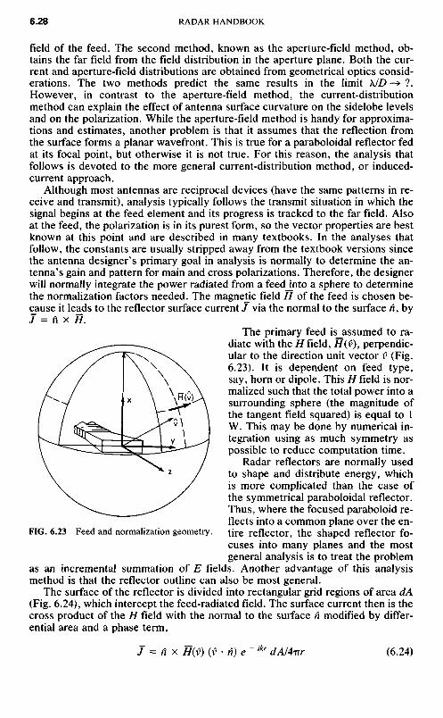
The primary feed is_assumed to ra-diate with the //field, H(V), perpendic-ular to the direction unit vector v (Fig.6.23). It is dependent on feed type,say, horn or dipole. This H field is nor-malized such that the total power into asurrounding sphere (the magnitude ofthe tangent field squared) is equal to 1W. This may be done by numerical in-tegration using as much symmetry aspossible to reduce computation time.

Radar reflectors are normally usedto shape and distribute energy, whichis more complicated than the case ofthe symmetrical paraboloidal reflector.Thus, where the focused paraboloid re-flects into a common plane over the en-tire reflector, the shaped reflector fo-cuses into many planes and the mostgeneral analysis is to treat the problem

as an incremental summation of E fields. Another advantage of this analysismethod is that the reflector outline can also be most general.

The surface of the reflector is divided into rectangular grid regions of area dA(Fig. 6.24), which intercept the feed-radiated field. The surface current then is thecross product of the H field with the normal to the surface n modified by differ-ential area and a phase term,

7 = n x H(v] (v • n) e " ikr dAl4vr (6.24)

FIG. 6.23 Feed and normalization geometry.

FIG. 6.24 Reflector geometry.

where r = the distance from the feed to the reflecting surface and k = 2ir/X = thewavenumber.

Each reflector grid region represents the reflection of a small uniformly illu-minated section. It has a gain factor and also a direction of reflection, which fol-lows Snell's law. The direction of reflection s can be written

s = v - 2 (n • v) n (6.25)

and the differential surface reflection at each grid region is modified by a patternfactor represented by a uniformly illuminated reflection steered in the direction ofunit vector s and determined in the pattern direction unit vector p by

4irc/A sin irbx(sx - px) sin TrAy(sy - py)Pattern factor = — (6.26)

\2\n - s\ TiAx(Sx - Px) TrAy(sy - py)

This factor modifies the surface current / as seen in the far field, projected in thedirection of interest. At a distant spherical surface, vector p is normal to the sur-face. Two vectors are determined at the surface for the polarizations of interest,both perpendicular to p and perpendicular to each other, considered main andcross-polarized directions. The dot product of each of these unit vectors with Jgives the field in the main and cross-polarized directions.

This pattern solution is found by a compromise between the number of gridregions and the time to compute all the parameters for each grid point. When thepattern is desired far off the pattern peak, one must consider the artificial gratinglobes created by the computation method itself, in which case the grid densitymust be increased. With grid size AJC, the artificially induced grating lobe will ap-pear at the angle found from sin 0 = XlAx. Frequently, the user of such compu-tational tools will trade off grid density in the orthogonal plane to enhance com-putation accuracy in the plane of interest.

Typically, the computer time-consuming operations in this type of patterncomputation are trigonometric functions, sines and cosines, and square rootsused in length and thus phase calculations. Extensive techniques are usually de-

vised to minimize repetitive calculations through the use of arrays containing theunit vectors in the pattern directions of interest, polarization vectors for thosedirections, and symmetry.

The literature contains many articles showing how geometric theory of diffrac-tion (GTD) techniques can be used to compute reflector patterns.7'39 The prob-lem one encounters with GTD is in generalizing the situation, such as an irregularantenna outline. The primary use one finds for GTD is in defining the antenna'soperation in the back hemisphere, but for many antennas the irregularity of theedges requires an agonizingly complex description of the antenna. This is oftenfound to be impractical to implement into a GTD analysis. Sometimes simpleanalyses are performed at special angles of interest.

6.6 SHAPED-BEAM ANTENNAS

Rotating search radars typically require antenna patterns which have a narrowazimuth beamwidth for angular resolution and a shaped elevation pattern de-signed to meet multiple requirements. When circular polarization is also one ofthe system requirements, a shaped reflector is almost always the practical choice,since circularly polarized arrays are quite expensive.

A typical range coverage requirement might look like that shown in Fig. 6.25.At low elevation angles, the maximum range is the critical requirement. Abovethe height-range limit intersection, altitude becomes the governing requirement,resulting in a cosecant-squared pattern shape. At still higher elevation angles,

RADAR SLANT R A N G E (nmi )FIG. 6.25 Typical two-way coverage requirement example.

HEIG

HT (

FEET

)

RANGELIMIT

HEIGHT LIMIT