185

Chapter 6

6. Optical Observations of Meteors Generating Infrasound –

II: Weak Shock Theory and Validation

A version of this chapter was submitted for a publication as:

Silber, E. A., Brown, P. G. and Z. Krzeminski (2014) Optical Observations of Meteors

Generating Infrasound – II: Weak Shock Model Theory and Validation, JGR-Planets,

submission # 2014JE004680

6.1 Introduction

6.1.1 Meteor Generated Infrasound

Well documented and constrained observations of meteor generated infrasound (Edwards

et al., 2008; Silber and Brown, 2014) are an indispensable prerequisite for testing,

validating and improving theoretical hypersonic shock propagation and prediction models

pertaining to meteors (e.g. ReVelle, 1974). However, due to the lack of a sufficiently

large and statistically meaningful observational dataset, linking the theory to observations

had been a challenging task, leaving this major area in planetary science underexplored.

Infrasound is low frequency sound extending from below the range of human hearing of

20 Hz down to the natural oscillation frequency of the atmosphere (the Brunt-Väisälä

frequency). Due to its negligible attenuation when compared to audible sound, infrasound

can propagate over extremely long distances (Sutherland and Bass, 2004), making it an

excellent tool for the detection and characterization of distant explosive sources in the

atmosphere. Infrasound studies have gained momentum with the implementation of the

global IMS network after the Comprehensive Nuclear Test Ban Treaty (CTBT) opened

for signature in 1996. The IMS network includes 60 infrasound stations, 45 of which are

186

presently certified and operational, designed with the goal of detecting a 1 kt (TNT

equivalent; 1 kt = 4.185 x 1018

J) explosion anywhere on the globe (Christie and Campus,

2010).

Included among the large retinue of natural (e.g. volcanoes, earthquakes, aurora,

lightning) (e.g. Bedard and Georges, 2000; Garces and Le Pichon, 2009) and

anthropogenic (e.g. explosions, re-entry vehicles, supersonic aircraft) (Hedlin et al.,

2002) sources of infrasound are meteors (ReVelle, 1976; Evers and Haak, 2001). A

number of meteoritic events have been detected and studied (e.g. Brown et al., 2008; Le

Pichon et al., 2008; Arrowsmith et al., 2008) since the deployment of the IMS network.

Often, no other instrumental records for these bolides are available; hence infrasound

serves as the sole means of determining the bolide location and energy. A notable

example of such an observation is the daylight bolide/airburst over Indonesia, which

occurred on 8 October, 2009 and produced estimated tens of kilotons in energy (Silber et

al., 2011).

Most recently, on 15 February, 2013, an exceptionally energetic bolide exploded over

Chelyabinsk, Russia, causing significant damage on the ground as well as a number of

injuries (Brown et al., 2013; Popova et al., 2013). Such events attest to the need to better

understand the nature of the shock wave produced by meteors.

The shocks produced by meteoroids may be detected as infrasound signals at the ground.

As meteoroids enter the Earth’s atmosphere at hypersonic velocities (11.2 – 72.8 km/s)

(Ceplecha et al., 1998), corresponding to Mach numbers from ~35 to 270 (Boyd, 1998),

they produce luminous phenomena known as a meteor through sputtering, ablation and in

some cases fragmentation (Ceplecha et al., 1998). Meteoroids can produce two distinct

types of shock waves which differ principally in their acoustic radiation directionality.

Their hypersonic passage through the atmosphere may produce a ballistic shock, which

radiates as a cylindrical line source. Episodes of gross fragmentation, where a sudden

release of energy occurs at a nearly fixed point (ReVelle, 1974; Bronshten, 1983) may

result in a quasi-spherical shock (e.g. Brown et al, 2007; ReVelle, 2010).

187

Meteoroids can produce two distinct types of shock waves which differ principally in

their acoustic radiation directionality. Their hypersonic passage through the atmosphere

may produce a ballistic shock, which radiates as a cylindrical line source. Episodes of

gross fragmentation, where a sudden release of energy occurs at a fixed point (ReVelle,

1974; Bronshten, 1983) may result in a quasi-spherical shock (e.g. Brown et al, 2007;

ReVelle, 2010).

Although infrasound does not suffer from significant attenuation over long distances, it is

susceptible to dynamic changes that occur in the atmosphere. Nonlinear influences,

atmospheric turbulence, gravity waves and winds, all have the potential to affect the

infrasonic signal as it propagates between the source and the receiver (Ostashev, 2002;

Kulichkov, 2004; Mutschlecner and Whittaker, 2010). Consequently, distant explosive

sources, such as bolides, are generally difficult to fully model or uniquely separate from

other impulsive sources based on infrasound records alone.

The first complete quantitative model of meteor infrasound was developed by ReVelle

(1974). In this model predictions are made, starting with a set of source parameters, for

the maximum infrasound signal amplitude and dominant period at the receiver. Due to a

lack of observational data, ReVelle’s (1974) cylindrical blast wave theory for meteors has

never been experimentally and observationally validated. In particular, regional (<300

km) meteor infrasound signals have been studied infrequently in favor of larger bolide

events, despite the fact that regional meteor infrasound is likely to reveal more

characteristics of the source shock, having been substantially less modified during the

comparatively short propagation distances involved (Silber and Brown, 2014).

A central goal of meteor infrasound measurements is to estimate the size of the relaxation

or blast radius (R0), as this is equivalent to an instantaneous estimate of energy

deposition, which is the key to defining the energetics in meteoroid ablation. Indeed, all

meteor measurements ultimately try to relate observational information back to energetics

either through light, ionization or shock (infrasound) production. In order to better define

meteoroid shock production, evaluate energy deposition mechanisms and estimate

meteoroid mass and energy, it is helpful to first investigate near field meteor infrasound

(ranges < 300 km) for well documented and characterized meteors, because this offers the

188

most plausible route in validating the cylindrical blast wave model of meteor infrasound.

Near field infrasonic signals are generally direct arrivals and suffer less from propagation

effects.

In this work, we attempt to validate the existing ReVelle (1974) meteor infrasound

theory, using a survey of centimeter-sized and larger meteoroids recorded by a multi-

instrument meteor network (Silber and Brown, 2014). This network, designed to optically

detect meteors which are then used as a cue to search for associated infrasonic signals,

utilizes multiple stations containing all sky video cameras for meteor detection and an

infrasound array located near the geographical centre of the optical network.

6.1.2 A Brief Review of ReVelle (1974) Meteor Weak Shock Theory

In the early 1950s, Whitham (1952) developed the F-function approach to sonic boom

theory, a novel method of treating the flow pattern of shock signatures generated by

supersonic projectiles, now widely used in supersonics and classical sonic boom theory

(e.g. Maglieri and Plotkin, 1991). It was soon realized that although the F-function offers

an excellent correlation between experiment and theory for low Mach numbers (< ~3), it

is not an optimal tool in the hypersonic regime (e.g. Carlson and Maglieri, 1972; Plotkin,

1989). Recently, the Whitham F-function theory has been applied to meteor infrasound

(Haynes and Millet, 2013), but it has not yet received a detailed observational validation.

We note, however, that this approach offers another theoretical pathway to predicting and

interpreting meteor infrasound, though we do not explore it further in this study.

Drawing on the early works of Lin (1954), Sakurai (1964), Few (1969), Jones et al.

(1968), Plooster (1968; 1970) and Tsikulin (1970), ReVelle (1974; 1976) developed an

analytic blast wave model of the nonlinear disturbance initiated by an explosive line

source as an analog for a meteor shock.

In cylindrical line shock theory, the magnitude of the characteristic blast wave relaxation

radius (R0) is defined as the region of a strongly nonlinear shock.

R0 = (E0/p0)1/2

(6.1)

189

Here, E0 is the energy deposited by the meteoroid per unit trail length and p0 is the

ambient hydrostatic atmospheric pressure. Physically this is the distance from the line

source at which the overpressure approaches the ambient atmospheric pressure. For a

single body ablating in the atmosphere, ignoring fragmentation, the blast radius can be

directly related to the drag force and ultimately expressed as a function of Mach number

(M) and meteoroid diameter (dm) (ReVelle, 1974):

R0 ~ M dm (6.2)

While the original ReVelle (1974) model assumes propagation through an isothermal

atmosphere, here we use an updated version incorporating a non-isothermal atmosphere.

As shown in an earlier study (Edwards et al., 2008), the isothermal approximation leads

to unrealistic values of signal overpressure. The following summary of ReVelle's (1974)

meteor infrasound theory is similar to that presented in Edwards (2010), though with

some corrections and emphasis on the approximations used by ReVelle (1974) and

aspects of the treatment most applicable to our study. The ReVelle (1974) approach

begins with a set of input parameters characterizing the entry conditions of the meteoroid,

and from these initial conditions predicts the infrasonic signal overpressure (amplitude)

and period at the ground. As part of this analysis, the blast radius and the height

(distortion distance) at which the shock transitions from the weakly nonlinear regime to

the linear regime is also determined. The model inputs are:

(i) station (observer) location (latitude, longitude and elevation);

(ii) meteoroid parameters (mass, density, velocity, and entry angle as measured

from the horizontal);

(iii) infrasonic ray parameters at the source which reach the station based on ray-

tracing results (angular deviation from the meteoroid plane of entry and shock

source location along the trajectory in terms of latitude, longitude and

altitude).

190

In the ReVelle (1974) meteor cylindrical blast wave theory the following assumptions are

made:

i. The energy release must be instantaneous.

ii. The cylindrical line source is valid only if v >> cs (the Mach angle has to be very

small many meteoroid diameters behind the body) and v = constant (Tsikulin,

1970). Therefore, it follows that if there is significant deceleration (v < 0.95ventry)

and strong ablation, the above criteria are not met and the theory is invalid.

iii. The line source is considered to be in the free field, independent of any reflections

due to finite boundaries, such as topographical features (ReVelle, 1974).

iv. Ballistic entry (no lifting forces present - only drag terms)

v. The meteoroid is a spherically shaped single body and there is no fragmentation

vi. The trajectory is a straight line (i.e. gravitational effects are negligible). The

nonlinear blast wave theory does not include the gravity term.

The coordinate system to describe the motion and trajectory of the meteoroid, as

originally developed by ReVelle (1974; 1976), is described in Chapter 2. In this model,

only those rays which propagate downward and are direct arrivals are considered (i.e.

direct source-observer path). The predicted signal period, amplitude and overpressure

ratio as a function of altitude are shown in Figure 6.1.

Note that due to severe nonlinear processes, the solutions to the shock equations are not

valid for x≤0.05, where x is the distance in units of blast radii (e.g. R/R0). Once the wave

reaches a state of weak nonlinearity (i.e. the shock front pressure (ps) ~ ambient pressure

(p0)), the shock velocity approaches the local adiabatic speed of sound (c). When ∆p/p0≤1

(at x≥1), weak shock propagation takes place and geometric acoustics becomes valid

(Jones et al., 1968; ReVelle, 1974). It is also assumed that at beginning, near the source

(x<1), the wave energy is conserved except for spreading losses (Sakurai, 1964).

191

Figure 6.1: The change in signal (a) amplitude, (b) period and (c) overpressure ratio

(dp/p0) as a function of height from source to receiver in a fully realistic atmosphere

(with winds and true temperature variations with height) according to the ReVelle (1974)

theory. In this case the meteor blast radius (R0) = 5 m, entry angle = 43°, speed = 29 km/s

and source height = 88.7 km.

Drawing upon theoretical and observational work on shock waves from lightning

discharges (Jones et al., 1968) the functional form of the overpressure has limiting values

of:

𝑓(𝑥)𝑥 → 0

=2(𝛾 + 1)

𝛾

Δ𝑝

𝑝0 → 𝑥−2 (6.3a)

and

𝑓(𝑥)𝑥 → ∞

= (3

8)−3/5

{[1 + (8

3)8/5

𝑥2]

3/8

− 1}

−1

→ 𝑥−3/4 (6.3b)

192

Here, γ is the specific heat ratio (γ=Cp/Cv=1.4) and ∆p/p0 is the overpressure. In the limit

as x → 0, where ∆p/p0 > 10, attenuation is quite rapid (x-2

), transitioning to x-3/4

as x → ∞,

where ∆p/p0 < 0.04 (or M = 1.017) (Jones et al., 1968). Taking advantage of equations

(3a) and (3b), and using results obtained from experiments (Jones et al., 1968; Tsikulin,

1970), the overpressure (for x ≥ 0.05) can be expressed as:

Δ𝑝

𝑝0=

2(𝛾 + 1)

𝛾(3

8)

−35

{

[1 + (8

3)

85𝑥2]

38

− 1

}

−1

(6.4a)

The limit within which this expression is applicable is 0.04 ≤ ∆p/p0 ≤ 10 (Jones et al.,

1968). The above expression can also be written as:

Δ𝑝

𝑝0≅

2𝛾

𝛾 + 1[

0.4503

(1 + 4.803𝑥2)38 − 1

] (6.4b)

After the shock wave has travelled a distance of approximately 10R0, where it is assumed

that strong nonlinear effects are no longer important, its fundamental period (τ0) can be

related to the initial blast radius via: τ0 = 2.81R0/c, where c is the local ambient

thermodynamic speed of sound. The factor 2.81 at x = 10 was determined experimentally

(Few, 1969) and found to compare favorably to numerical solutions (Plooster, 1968). The

frequency of the wave at maximum is referred to as the ‘dominant’ frequency (ReVelle,

1974). For a sufficiently large R, and assuming weakly nonlinear propagation, the line

source wave period (τ) for x ≥ 10 is predicted to increase with range as:

𝜏(𝑥) = 0.562 𝜏0 𝑥1/4 (6.5)

Far from the source, the shape of the wave at any point will mainly depend on the two

competing processes acting on the propagating wave: dispersion, which reduces the

overpressure and ‘stretches’ the period; and steepening, which is the cumulative effect of

small disturbances, tending to increase the overpressure amplitude (ReVelle, 1974). In

ReVelle’s (1974) model, however, it is assumed that the approximate wave shape is

known at any point. After a short distance beyond x = 10, the waveform is assumed to

remain an N-wave (DuMond et al., 1946) type-shape (ReVelle, 1974).

193

For the analytic implementation of ReVelle's theory, it is necessary to choose some

transition distance from the source where we consider the shock as having moved from

weakly nonlinear propagation to fully linear. The precise distance at which the transition

between the weak shock and linear regime occurs is poorly defined. Physically, it occurs

smoothly, as no finite amplitude wave propagating in the atmosphere is truly linear; this

is always an approximation with different amplitudes along the shock travelling with

slightly different speeds. This distance was originally introduced by Cotten et al. (1971)

in the context of examining acoustic signals from Apollo rockets at orbital altitudes.

Termed by Cotten et al. (1971) the "distortion distance", it is based upon Towne’s (1967)

definition of the distance (d') required for a sinusoidal waveform to distort by 10%.

ReVelle (1974) adopted this distance, together with the definition of Morse and Ingard

(1968), to define the distance (ds) an initially sinusoidal wave must travel before

becoming "shocked". Thus, it follows that ds = 6.38 d', where d' > da and da is the

remaining propagation distance of the disturbance before it reaches the observer. Further

details summarizing the ReVelle (1974) model are given in Chapter 2.

In summary, according to the ReVelle (1974) weak shock model, there are two key sets

of expressions to estimate the predicted infrasonic signal period and the amplitude at the

ground. The first is the expression for the predicted dominant signal period in the weak

shock regime (d'≤da). Once the shock is assumed to propagate linearly, by definition the

period remains fixed.

The second expression relates to the overpressure amplitude. In the weak shock regime

the predicted maximum signal amplitude is given by:

Δpz→obs = ( f(x) Dws(z) N*(z) Z

*(z) ) p0 (6.6a)

where f(x) is the expression given in equation (4b), N* and Z* are the correction factors

as described in Chapter 2 and Dws is the weak shock damping coefficient.

Once the wave transitions into a linear wave, the maximum signal amplitude is given by:

Δ𝑝𝑧→𝑜𝑏𝑠 = [Δ𝑝𝑧→𝑡 𝐷𝑙(𝑧)𝑁∗(𝑧)𝑧→𝑜𝑏𝑠 𝑍

∗(𝑧)𝑧→𝑜𝑏𝑠

𝑁∗(𝑧)𝑧→𝑡 𝑍∗(𝑧)𝑧→𝑡 (

𝑥𝑧→𝑡

𝑥𝑧→𝑜𝑏𝑠)1/2

] 𝑝0 (6.6b)

194

where Δpz→t is identical to the expression given in equation (6a) and Dl is the linear

damping coefficient. The subscripts z, t and obs in equations (6a) and (6b) denote the

source altitude, transition altitude and the receiver’s altitude, respectively, following the

notation in ReVelle (1974).

The ReVelle (1974) model as just described has been coded in MATLAB® to allow

comparison between the predicted amplitudes and periods of meteor infrasound at the

ground with the observations, the focus of this paper. In our first paper in the series

(Silber and Brown, 2014 in review), we used optical measurements to positively identify

infrasound from specific meteors and constrain the point (and its uncertainty) along the

meteor trail where the observed infrasound signal emanated. That work also examined

the influence of atmospheric variability on near-field meteor infrasound propagation and

established the type of meteor shock production at the source (spherical vs. cylindrical).

We also developed a meteor infrasound taxonomy using the pressure-time waveforms of

all the identified meteor events as a starting point to gain insight into the dominant

processes which modify the meteor infrasound signal as observed at the ground.

Here, we use the dataset constructed in the first part of our study and select the best

constrained (ie. those for which we have accurate infrasound source heights) meteor

events to address the following:

i. for meteors detected optically and with infrasound, use the ReVelle (1974) weak

shock theory to provide a bottom-up estimate of the blast radius (i.e. from

observed amplitude and period at the ground can we self-consistently estimate the

blast radius at the source);

ii. test the influence of atmospheric variability, winds, Doppler shift and initial shock

amplitude on the weak shock solutions within the context of ReVelle (1974)

meteor infrasound theory;

iii. determine an independent estimate of meteoroid mass/energy from infrasonic

signals alone and compare to photometric mass/energy measurements;

195

iv. critically evaluate and compare ReVelle’s (1974) weak shock theory with

observations, establishing which parameters/approximations in the theory are

valid and which may require modification.

6.2 Methodology and Results

6.2.1 Weak Shock: Model Updates and Sensitivities

The ReVelle (1974) weak shock model algorithm was implemented in MATLAB®

and

updated to include full wind dependency, as well as Doppler shift for period (Morse and

Ingard, 1968) as a function of altitude. The influence of the winds is reflected in the

effective speed of sound (ceff), which is given by the sum of the adiabatic sound speed (c)

and the dot product between the ray normal (�̂�) and the wind vector (�⃑� ):

𝑐𝑒𝑓𝑓 = 𝑐 + �̂� ∙ �⃑� (6.7)

The signal amplitude is affected by winds such that the amplitude will intensify for

downwind propagation and diminish in upwind propagation (Mutschlecner and

Whittaker, 2010). In the linear regime, the signal period (equation 6.5), does not suffer

any decay with distance, but the winds do induce a Doppler shift. Following Morse and

Ingard (1968), the Doppler shift due to the wind is given by:

Ω = 𝜔 − �⃑� ∙ �⃑� (6.8)

where Ω is the intrinsic angular frequency (frequency in the reference frame of the

moving wind with respect to the ground), ω is the angular frequency in the fixed earth

frame of reference and �⃑� is the wave number. Since the contribution of winds in the

vertical direction is generally 2-4 orders of magnitude smaller than the horizontal wind

contribution (Wallace and Hobbs, 2006; Andrews, 2010), it is neglected.

Another addition to the weak shock model was the inclusion of updated absorption

coefficients (Sutherland and Bass, 2004), applicable in the linear propagation regime.

In the first part of our study (Silber and Brown, 2014) we described the influence on the

raytracing results of small scale perturbations in the wind profile due to gravity waves on

raytracing results. While the effects were small, they were significant enough to produce

196

propagation paths which were non-existent using the average atmosphere from the source

to the receiver. Here we have used the same ‘perturbed’ atmospheric profiles to test the

influence of gravity-wave-induced perturbations on the predicted signal amplitude and

period as calculated using the weak shock model. We selected five events which span the

global range of our final data (i.e. meteors with different entry velocity, blast radius, and

shock heights), and ran the weak shock code using 500 ‘perturbed’ atmospheric profiles.

For each event and each realization we computed the magnitude of the modelled

infrasonic signal period and amplitude while simultaneously testing the effect of different

absorption coefficients in the linear regime using the set given by ReVelle (1974) and

that of Sutherland and Bass (2004).

The overall effect of both winds and Doppler shift on the weak shock model was found to

be relatively small, resulting in R0 differences of no more than 13% for the period

(average 4%) and as high as 9% for the amplitude (average 3%). The perturbations to the

atmospheric winds expected from gravity-waves were found to have even smaller effects

on estimates of R0, typically of 10% or less.

In addition, the predicted ground-level period and amplitude outputs of the weak shock

model were tested using a synthetically generated meteor (Figure 6.2).

197

Figure 6.2: An example of the predicted ground-level amplitude and period of a meteor

shock using the ReVelle (1974) theoretical model. In these figures, the meteor moves

northward, as shown with the arrow in each plot, starting ablation at an altitude of 90 km

and ending at 40 km. A representative realistic atmosphere was applied, accounting for

the wind. The top two panels show the predicted (a) linear and (b) weak shock amplitude.

The bottom two panels show the predicted (c) linear and (d) weak shock period. The

amplitude in the linear regime has a larger magnitude than that in the weak shock regime,

while the opposite is true for the signal period. The synthetic meteor parameters are

shown in the lower right of plot (b).

198

6.2.2 Weak Shock: Bottom-up Modelling

The first approach we adopt to testing the ReVelle (1974) theory is a bottom-up

methodology. This provides an indirect method of estimating the blast radius at the

meteor using infrasound and optical astrometric measurements of the meteor only (i.e.

without prior independent knowledge of the meteoroid mass and density). Given the

input parameters, all of which are known except the blast radius, the goal is to answer the

following question: what is the magnitude of the blast radius required to produce the

observed signal amplitude and period at the station if we assume (i) the signal remained a

weak shock all the way to the ground and (ii) if it transitioned to the linear regime?

Additionally, we want to define the blast radius uncertainty given the errors in signal

measurements.

Drawing upon the results obtained in Silber and Brown (2014), the 24 well constrained

optical meteors which were also consistent with cylindrical line sources (as determined

through optical measurements and raytracing) were used to observationally test the weak

shock model. The orbital parameters and meteor shower associations for our data set are

listed in Table 6.1. Out of these 24 events, 18 produced a single infrasonic arrival, while

six events produced two distinct infrasonic arrivals at the station. The meteor shock

source altitude in our data set ranges from 53 km to 103 km, the observed signal

amplitude (Aobs) is from 0.01 Pa to 0.50 Pa, while the observed dominant signal period

(τobs) is between 0.1 s and 2.2 s. Typical values of overpressure from meteors in this study

are 1-2 orders of magnitude smaller than those associated with the signals from Apollo

rockets as reported by Cotten et al. (1971), the last comparable study to this one.

For the model to be self-consistent a single blast radius should result from the period and

amplitude measurements. In practice, we find estimates of blast radii for period and

amplitude independently in both linear and weak shock regimes such that the measured

signal amplitude or period is matched within its measurement uncertainty. Therefore, for

each amplitude/period measurement there are two pairs of theoretical quantities produced

from ReVelle's (1974) theory: the predicted signal amplitude (Aws) and period (τws) in the

weak shock regime, and the signal amplitude (Al) and period (τl) in the linear regime. The

iterations began with a seed-value of the initial R0, and then based on the computed

199

results the process is repeated with a new (higher or lower) value of R0 and the results

again compared to measurements until convergence is reached. The result of this bottom-

up procedure is a global estimate of the blast radius matching the observed amplitude or

period assuming either weak-shock or linear propagation (Aws, τws, Al, τl). In the second

phase of this bottom-up approach, this global modelled initial blast radius was used as an

input to iteratively determine the minimum and maximum value of the model R0 required

to match the observed signal (period or amplitude) within the full range of measurement

uncertainty.

Table 6.1: A summary of orbital parameters for all events in our data set. The columns

are as follows: (1) event date, (2) Tisserand parameter, a measure of the orbital motion of

a body with respect to Jupiter (Levison, 1996), (3) semi-major axis (AU), (4) eccentricity,

(5) inclination (°), (6) argument of perihelion (ω) (°), (7) longitude of ascending node (°),

(8) geocentric velocity (km/s), (9) heliocentric velocity (km/s), (10) α – right ascension of

geocentric radiant (°), (11) δ – declination of geocentric radiant (°), (12) perihelion (AU),

(13) aphelion (AU), (14) meteor shower associations. The meteor shower codes are: α-

Capricornids (CAP), Orionids (ORI), Perseids (PER), and Southern Taurids (STA). Note

all angular quantities are J2000.0.

1 2 3 4 5 6 7 8 9 10 11 12 13 14

Date Tiss a e inc ω asc node vg vh α geo δ geo q per q aph Showers

20060419 2.8 3.2 0.69 2.2 195.5 29.021 10.0 38.6 153.0 20.2 0.989 5.4 --

20060805 hyp -8.4 1.12 144.9 164.9 132.716 69.0 43.1 38.7 37.1 0.996 -17.7 --

20061104 3.1 2.2 0.83 4.3 292.1 221.472 28.0 37.3 49.0 22.0 0.371 4.1 --

20070125 hyp -1.7 1.57 156.4 342.6 124.950 76.6 48.3 214.3 -28.9 0.957 -4.3 --

20070727 2.7 2.8 0.80 8.3 269.9 123.717 23.8 37.8 303.7 -9.3 0.566 5.1 CAP

20071021 1.2 2.5 0.80 172.9 94.6 27.535 63.4 37.9 95.6 20.1 0.519 4.6 ORI

20080325 3.7 1.9 0.48 7.3 358.8 184.634 7.7 36.3 95.8 -13.2 0.997 2.9 --

20080511 hyp -26.1 1.03 9.3 42.6 230.738 19.6 42.3 191.2 -25.4 0.874 -53.1 --

20080812 1.0 3.7 0.74 110.8 157.7 139.878 56.4 38.9 41.3 57.8 0.981 6.4 PER

20081028 2.7 3.2 0.71 6.9 31.6 34.961 12.1 38.8 2.4 -23.0 0.932 5.4 --

20081102 3.5 1.8 0.82 5.2 118.2 40.086 27.9 36.1 52.7 14.6 0.335 3.3 STA

20081107 hyp -8.8 1.11 152.8 10.0 45.144 71.5 43.5 130.2 1.7 0.983 -18.7 --

20090428 3.1 2.4 0.68 10.6 244.7 37.916 18.0 37.3 211.2 8.9 0.773 4.1 --

20090523 hyp -41.8 1.02 21.3 250.7 62.169 27.9 42.1 240.2 6.4 0.671 -84.3 --

20090812 0.5 5.4 0.82 111.9 154.0 139.617 57.5 39.8 44.0 57.8 0.967 9.8 PER

20090917 2.5 3.2 0.81 0.3 263.0 174.168 22.4 38.6 350.9 -3.4 0.610 5.8 --

20100421 0.4 93.7 0.99 71.7 257.8 30.847 45.3 41.9 252.1 21.2 0.610 186.9 --

20100429 1.0 5.8 0.85 82.8 229.2 38.658 47.2 40.1 274.4 27.9 0.846 10.8 --

20100530 2.5 3.0 0.86 4.6 284.4 68.652 28.2 38.1 254.4 -18.4 0.429 5.6 --

20110520 2.6 3.2 0.78 6.0 252.8 58.759 20.9 38.5 229.8 -8.5 0.699 5.8 --

20110630 1.5 7.9 0.87 45.0 187.8 97.886 28.6 40.4 274.9 61.5 1.012 14.7 --

20110808 2.3 3.8 0.74 37.1 156.9 135.191 24.2 38.9 223.8 70.6 0.980 6.6 --

20111005 2.6 2.8 0.85 7.9 103.2 11.464 27.2 38.2 19.9 0.1 0.437 5.2 --

20111202 2.9 2.4 0.81 5.5 100.8 69.314 26.0 37.9 74.8 16.8 0.461 4.4 --

200

The summary of the bottom-up blast radius modelling results are presented in Figure 6.3.

There is a significant discrepancy between the period-based blast radii and amplitude-

based blast radii in both the linear and weak shock regimes. The average blast radius

from amplitude determinations in the linear regime is approximately 30 times smaller

than that in the weak shock regime, indicating that the transition to linearity approach

employed in the ReVelle (1974) weak shock model perhaps significantly underestimates

the blast radius. In the weak shock regime, where we assume the signal can be treated as

a weak shock all the way to the ground, we find that the amplitude-estimated R0 in most

cases is larger than that estimated from the period, but the difference is much smaller than

the linear case, being no more than a factor of 15 between the amplitude and period.

Almost half of the events show agreement within uncertainty.

Figure 6.3: The behaviour of R0 in (a) linear and (b) weak shock regimes in the bottom-

up modelling approach. In the linear regime, the amplitude blast radius appears

underestimated relative to the R0 estimated from the period, while in the weak shock

regime, the behaviour is reversed. In all plots, the blue line represents the 1:1

correspondence, while the red line is the best fit.

201

6.2.3 Weak Shock: Top-Down Modelling

6.2.3.1 Photometric Measurements

The fundamental equations of motion (Bronshten, 1983; Ceplecha et al., 1998) for a

meteoroid of mass m and density ρm entering the Earth’s atmosphere at velocity v are

given by the drag and mass-loss equations:

𝑑𝑣

𝑑𝑡= −

Γ𝐴𝜌𝑎𝑣2

𝑚13𝜌𝑚

23

(6.9)

𝑑𝑚

𝑑𝑡= −

ΛA𝜌𝑎𝑣3𝑚

23

2𝜉𝜌𝑚

23

(6.10)

Here, Γ is a drag coefficient, 𝜉 is the heat of ablation of the meteoroid material (or energy

required to ablate a unit mass of the meteoroid), Λ is the heat transfer coefficient, which

is a measure of efficiency of the collision process in converting kinetic energy into heat

(McKinley, 1961), ρa is density of the air, and A is the dimensionless shape factor (Asphere

= 1.209).

The all-sky meteor camera system used for this survey and details of the astrometric

reductions and measurements methodology are presented in Silber and Brown (2014).

Here we briefly describe the photometric analysis.

A series of laboratory experiments were performed to determine the camera response in

an effort to model the effects of camera saturation (which affect many of our events). In

the field, measurements were performed to model the lens roll-off (the apparent drop in

sensitivity of the camera as the edges of the all-sky field are reached). The lens roll-off

correction becomes significant for meteors as a >0.8 astronomical magnitude attenuation

results for elevations below ~15 degrees. Other standard photometric corrections were

applied including extinction correction (e.g. Vargas et al., 2001; Burke et al., 2010) and

apparent instrumental magnitude converted to an absolute magnitude by referencing all

meteors to a standard range of 100 km (McKinley, 1961).

202

Bright meteors (magnitude > -4) are typically saturated on the 8-bit cameras. In our

laboratory setup, an artificial star of variable brightness was created using a fixed light

source and a turning wheel with a neutral density filter of varying density following the

procedure used by Swift et al. (2004). Standard photometric procedures (Hawkes, 2002)

were used to determine the apparent instrumental magnitude of the artificial star and a

power law fit between the observed and known brightness of the artificial star was then

computed to find a correction for the saturation which we applied to meteors to deduce

their true apparent magnitude.

The instrumental magnitude of any given star (or meteor) varies as a function of distance

from the optical center (or zenith distance if the camera is vertically directed) of the

camera lens. For our cameras a star appears about 2.5 stellar magnitudes dimmer near the

horizon than at the zenith due to the natural vignetting in the optical system. The in-field

experiment was performed on a clear night by setting up the camera on a turntable

attached to a fixed frame and taking a series of video frames starting from the horizon

and sweeping through an angle of 180° through the zenith. Several bright stars then had

their instrumental magnitudes computed as a function of distance from the optical axis to

compute the lens roll-off which was found to functionally behave as cos4θ. Applying all

these corrections we then followed standard photometric routines (Hawkes, 2002), to

compute the light curves for each meteor in our instrumental passband. Our cameras use

hole accumulation diode CCD chips (Weryk and Brown, 2013). The CCDs have both a

wide passband and high QE making them extremely sensitive in low-light conditions.

Our limiting meteor sensitivity is approximately MHAD = -2 corresponding to meteoroids

of ~5 g or roughly 1cm in diameter at 30 km/s.

There are two approaches which can be used to determine the mass of a meteoroid given

optical data. First, we may appeal to empirical estimates of the magnitude-mass-speed

determined from earlier photographic surveys (e.g. Jacchia et al. (1967)) which yields:

MHAD = 55.34 – 8.75 log v - 2.25 log m – 1.5 log cos ZR (6.11)

where MHAD is the absolute magnitude in the HAD bandpass, m is the mass of the

meteoroid in grams, ZR is the zenith angle of the radiant and where the meteoroid velocity

(v) is expressed in cgs units. The original relation was computed in the photographic

203

bandpass. We estimated the color correction term between our instrumental system and

the photographic system, (MHAD = MPh+1.2) by assuming each meteor radiates as a

4500K blackbody and computing the energy falling into our HAD bandpass as compared

to the photographic bandpass following the synthetic photometry procedure described in

Weryk and Brown (2013).

A second approach to estimate photometric mass is to directly integrate the light emission

(I) of the meteoroid throughout the time of its visibility:

𝑚 = 2∫ 𝐼𝑑𝑡

𝜏𝐼𝑣2 (6.12)

where τI is the luminous efficiency defined as the fraction of the meteoroid’s kinetic

energy produced converted into radiation (Ceplecha et al., 1998). More about this

approach can be found in Ceplecha et al. (1998) and Weryk and Brown (2013).

The magnitude of the blast radius at any point along the meteor trail can be thought of as

a ‘snapshot’ of the energy per unit path length deposited into the atmosphere by a

meteoroid. This may also be equated to the meteoroid mass times the Mach number at

that point assuming single body ablation (ReVelle, 1976).

While the single body approach is much more simple if the source region along the trail

where the shock observed at the microphone location on the Earth’s surface is produced

close to the end of the meteor trail the total initial photometric mass poorly represents the

actual energy/mass at the source location. If the initial mass is used to test the weak shock

model, it produces erroneous results as the actual mass (and energy deposited per unit

path length) would be much smaller as the initial meteoroid mass is much larger than the

remnant mass near the end of the trail.

6.2.3.2 The Fragmentation (FM) Model

A third approach to estimating mass using optical data is to apply an entry model code to

fit the observed brightness and length vs. time measured for the meteor. Here we use the

fragmentation (FM) model of meteoroid motion, mass loss and radiation in the

atmosphere (Ceplecha and ReVelle, 2005) to fit the observed brightness and length vs.

time measured for the infrasound-producing meteor. As fragmentation is explicitly

204

accounted for, the FM model should provide a more realistic estimate of energy

deposition along the trail, and thus R0.

The first step in constructing an entry model solution was to begin with the approximate

(starting) values for intrinsic shape density coefficient (K) and intrinsic ablation

coefficient (σ), which are defined by the following expressions (Ceplecha and ReVelle,

2005):

𝜎 =Λ

2𝜉Γ (6.13)

𝐾 =ΓA𝑠

𝜌2/3 (6.14)

The intrinsic shape density coefficient (K) and intrinsic ablation coefficient (σ) are then

modified together with the initial mass in a forward modeling process. We do this

statistically by first classifying each of our meteors according to the fireball types defined

by Ceplecha and McCrosky (1976) (hereafter CM). This is done by calculating the PE

parameter (Ceplecha and McCrosky, 1976), defined as:

PE = log ρE + A0 log m + B0 log v + C0 log cos ZR (6.15)

where ρE is the density of air (in cgs units) at the trajectory end height, m is the estimated

initial mass in grams, and the meteoroid entry velocity (v) is expressed in km/s. From fits

to a large suite of photograhphically observed fireballs, CM found A0 = -0.42, B0 = 1.49

and C0 = -1.29. As an estimate for the initial mass we use the mass computed from

equation (6.31) and assume a +1.2 color term between the HAD and photographic

bandpasses. In this way we derive estimates for the PE for each of our events. The range

of values of PE and presumed corresponding meteoroid types as proposed by CM are

given in Table 6.2. The observed light curve from photometric measurements, in

conjunction with the astrometric solution (event time, path length as a function of height

and entry angle) for each event, was used to match the theoretical light curve and model

length vs. time to observations through forward modelling (Figure 6.4).

As our average meteoroid mass is intermediate between fireball and small camera data,

we a priori expect our distribution of fireball types (I-III) to be intermediate between

205

these two classes, if our mass scale is reasonable. As shown in Table 6.2, within the

limitations of our small number statistics, our distribution is broadly consistent with

being intermediate between the percentage distribution of these two categories given by

Ceplecha et al. (1998) indicating our choice of color term is physically reasonable.

Table 6.2: The range of PE parameter and the associated meteoroid group presumed type,

type of the material and representative density as given by Ceplecha et al. (1998). The

percentage of observed meteoroids in each group according to mass category typical of

fireball networks (mass range 0.1 - 2000 kg) and small cameras (mass range 10-4

kg to

0.5 kg) as published in (Ceplecha et al., 1998) and the percentages found in this study

(masses 10-4

kg to 1.0 kg). The range of values for σ and K found in our study within the

framework of the FM model are given in the last two columns.

PE rangeGroup

type

Type of the

meteoroid

material

ρm

(kg/m3)

%

observed

(fireball

networks)

%

observed

(small

cameras)

%

observed

(this

study)

σ K

PE > -4.6 I

ordinary

chondrites,

asteroids

3700 29 5 130.006-

0.021

0.46-

1.29

-4.6 ≥ PE

> -5.25II

carbonaceous

chondrites,

comets,

asteroids

2000 33 39 370.002-

0.19

0.1-

3.09

PE ≤ -5.7 IIIbsoft cometary

material270 9 19 37

0.001-

0.06

1.2-

4.89

130.002-

0.009

1.93-

3.29

-5.25 ≥

PE > -5.7IIIa

regular

cometary

material

750 26 41

206

Figure 6.4: The FM model fit to the light curve for a multi-station meteor recorded at

07:05:56 UT on 19 April 2006. The model is matched in both (a) magnitude vs. time and

(b) height residuals vs. time (dynamic fit). In this case the FM model provides a best fit

of 14.18 km/s initial speed and 20 g mass. Full details can be found in Table 6.3.

Depending on the shape of the light curve (e.g. obvious flares or a smooth light curve),

the model is used to implement either a single body approach or discrete fragmentation

points. Using the results for 15 bolides obtained by Ceplecha and ReVelle (2005) as a

starting reference point, the following parameters were forward modeled until a best fit to

the observed light curve as well as magnitude as a function of height and path length

were found: K, σ, integration altitude, the initial mass, the mass loss at each

fragmentation point (if applicable), duration of the flare, interval from the start of the

flare until the flare maximum and part of mass fragmented as large fragments. From the

model we have the following to match to the meteor: time, path length, altitude, velocity,

dv/dt, mass, dm/dt, meteor luminosity, meteor magnitude, σ, K, luminous efficiency and

zenith distance of the radiant. The summary of photometric and dynamic masses, as well

as meteoroid types, is given in Table 6.3. While the FM model performs very well in

matching the observed light curves, it should be noted that the final solution is

representative, but not necessarily unique. For example, if the shape coefficient is

increased, then similar output results are found by reducing the initial mass. These

differences in initial parameters and their variation at fragmentation points may result in

an uncertainty of up to factor of several in the initial mass and therefore affect the mass

207

loss in a similar fashion as a function of altitude. The ranges of the σ and K values used

for modelling are given in Table 6.3.

In the general case, the energy lost by the meteoroid per unit path length is:

𝑑𝐸

𝑑𝐿= (

𝑣2

2

𝑑𝑚

𝑑𝐿+ 𝑚𝑣

𝑑𝑣

𝑑𝐿) (6.16)

To determine the blast radius using the dynamics from the FM model, we applied

equation (6.16), also accounting for mass loss during fragmentation episodes, or single-

body mass at the height corresponding to the shock height.

208

Table 6.3: A summary of the photometric mass measurements using observed light

curves from meteor video records. The columns are as follows (column numbers are in

the first row): (1) meteor event date, (2) meteor velocity (km/s) at the onset of ablation,

(3) begin height (km), (4) end height (km), (5) instrument corrected peak magnitude

(MHAD) from the observed light curve, (6-7) minimum and maximum values of shape

coefficient (K) (in c.g.s. units), and (8-9) minimum and maximum values of ablation

coefficient (σ) (s2/km

2) used in the FM model fitting, (10) estimated meteor mass (g)

from equation (6.30), (11) estimated meteor mass (g) using integrated light curve, (12)

initial (entry) meteor mass (g) from the FM model, (13) PE coefficient and (14)

meteoroid group type.

6.2.3.3 Top-Down Weak Shock Modelling

To perform the top-down weak shock modelling, we start at the "top" by using the FM

model estimates for R0 in conjunction with the other optically measured parameters for

each meteor and calculate the predicted signal period and amplitude at the ground,

assuming both weak shock and linear propagation. This provides an independent

1 2 3 4 5 6 7 8 9 10 11 12 13 14

Date

Entry

Velocity

(km/s)

H

begin

(km)

H

end

(km)

Peak

Mag K min K max σ min σ max

Mass

(JVB) (g)

Mass

(int) (g)

FM

Model

Mass (g) PE Type

20060419 14.2 72.0 47.7 -2.7 0.14 0.53 0.009 0.009 107.4 23.5 20.0 -4.69 II

20060805 67.5 126.4 74.5 -12.8 1.4 2.3 0.002 0.004 5927.6 432.9 74.0 -6.20 IIIB

20061104 30.3 89.9 65.8 -7.2 1.8 4.18 0.002 0.005 459.9 12.5 12.0 -6.39 IIIB

20070125 71.2 119.2 88.5 -5.9 1.99 3.69 0.001 0.004 9.5 2.7 0.9 -5.12 II

20070727 26.3 96.2 70.6 -8.2 0.46 2.68 0.002 0.004 2583.9 91.5 63.0 -6.22 IIIB

20071021 64.3 130.8 81.7 -8.8 2.5 2.5 0.004 0.004 57.5 10.6 4.3 -5.82 IIIB

20080325 13.5 76.2 32.8 -5.9 0.69 0.79 0.015 0.015 2912.0 792.9 917.0 -4.51 I

20080511 23.5 95.2 77.3 -3.8 2.54 2.54 0.06 0.06 85.8 5.2 8.0 -5.90 IIIB

20080812 56.6 105.7 82.0 -1.8 3.29 -- 0.009 -- 0.2 0.1 0.1 -4.93 II

20081028 15.4 81.2 41.1 -4.1 0.66 0.66 0.014 0.014 309.8 79.6 110.0 -4.40 I

20081102 30.1 96.5 62.6 -7.7 1.73 2.05 0.002 0.002 663.9 53.3 18.0 -5.58 IIIA

20081107 71.6 113.5 81.5 -3.1 1.99 2.59 0.003 0.006 0.4 0.2 0.1 -4.56 I

20090428 21.2 83.5 38.0 -7.2 0.14 1.09 0.003 0.005 3086.5 784.1 330.0 -4.77 II

20090523 29.9 95.9 72.4 -2.0 0.2 0.86 0.042 0.044 2.7 0.7 2.2 -5.10 II

20090812 58.7 108.5 80.4 -6.7 1.29 3.29 0.008 0.01 20.6 3.4 1.8 -5.65 IIIA

20090917 24.2 85.7 72.4 -2.7 3.05 3.05 0.004 0.004 20.7 6.6 8.5 -5.31 IIIA

20100421 45.9 108.5 74.6 -9.3 1.5 1.5 0.005 0.0055 861.5 45.7 17.0 -5.95 IIIB

20100429 47.7 105.7 89.9 -2.6 4.89 4.89 0.014 0.014 0.9 0.2 0.3 -5.79 IIIB

20100530 29.3 96.0 78.3 -0.8 2.19 2.99 0.01 0.012 1.2 0.3 0.3 -5.12 II

20110520 22.5 95.7 84.1 -3.1 2.79 2.99 0.039 0.039 21.3 2.3 2.5 -6.35 IIIB

20110630 29.8 100.5 71.7 -7.8 2.49 2.49 0.003 0.003 527.5 18.0 10.0 -6.05 IIIB

20110808 25.5 86.6 39.9 -9.3 0.99 1.49 0.002 0.002 9990.9 2586.4 1003.0 -4.77 II

20111005 28.5 96.2 64.5 -2.9 1.09 1.59 0.004 0.004 6.8 2.6 20.0 -4.78 II

20111202 27.6 97.0 53.8 -3.1 0.29 0.69 0.008 0.009 18.0 8.8 9.0 -4.06 I

209

comparison between the bottom-up modeling and forms a potential cross-calibration

between infrasonically derived energy/mass and the same photometrically estimated

quantities.

Figure 6.5 shows the comparison of the blast radius as obtained via FM model versus the

blast radius from bottom-up modelling including all four outputs (the period and

amplitude in linear and weak shock regimes). In the linear regime, the amplitude-based

R0 from the bottom-up modelling is clearly underestimated compared to the R0 derived

from the FM model. The comparison between the predicted signal period and amplitude

using R0 from the top-down modelling and that observed is shown in Figure 6.6. The

predicted signal amplitude is somewhat underestimated in the weak shock regime and

markedly overestimated in the linear regime. The predicted signal period, however,

shows a near 1:1 agreement with the observed period.

Figure 6.5: The blast radius estimated from bottom-up modelling as compared to blast

radii derived from application of the FM model. Tlin and Tws are the period in linear and

weak shock regime, respectively. Alin and Aws are the amplitude in linear and weak

shock regime, respectively.

210

Figure 6.6: (a) Signal period and (b) amplitude obtained by running the top-down weak

shock model with input R0 as derived via FM model.

6.2.4 Infrasonic Mass

From the optical measurements of the meteor and appealing to the fireball classification

work of Ceplecha and McCrosky (1976) it is possible to correlate the fireball type with

its likely physical properties (i.e. density) (Ceplecha et al., 1998) (Table 6.2) and thus

compute an infrasonic mass (Edwards et al., 2008) through m = πρdm3/6, assuming a

spherical shape and single body ablation (i.e. no fragmentation) from the bottom-up

modelling. Using equation (6.2) and the relationship between the meteoroid density and

diameter, infrasonic mass (minfra) is then given by:

m𝑖𝑛𝑓𝑟𝑎 = πρ

6(𝑅0

𝑀)3

(6.17)

Considering that the bottom-up modelling yields four values of blast radii as described in

section 6.2.2, there are four resultant infrasonic masses. These are compared to

photometric masses derived through the FM model (Figure 6.7). The infrasonic masses

derived from the period-based R0 are in better agreement with the photometric masses

than are the infrasonic masses derived from the amplitude-based R0 in either regime.

Drawing upon equation (6.1), meteoroid energy can be derived from R0 (bottom-up and

top-down) without needing to make any assumption about single body (Figure 6.8).

211

Figure 6.7: The comparison of the infrasonic and photometrically derived masses. The

abscissa in both panels represents the equivalent photometric mass derived from the FM

model blast radius and equation (6.17). The infrasonic masses derived from the

amplitude-based (top panel) and period-based (bottom panel) blast radius in the linear

and weak shock regimes are shown. The grey line is the 1:1 line in all plots.

212

Figure 6.8: Energy per unit path length comparison between the bottom-up modelling,

where R0 is determined entirely from the infrasound signal properties at the ground, and

the FM model. The grey line is the 1:1 line.

6.3 Discussion

The linear amplitude-derived R0 was on average 12% larger when the Sutherland and

Bass (2004) coefficients were applied. To put this in perspective, the range of R0 from

matching the amplitude in the linear regime was from 0.15 m to 7.4 m with the

Sutherland and Bass (2004) coefficients and from 0.09 m to 7 m using the classical

coefficients (ReVelle, 1974). The most significant difference was found for signals with a

dominant frequency > 12 Hz (at the weak shock to linear regime transition altitude point).

However, even in this case, the difference is still within the uncertainty bounds in R0 fits.

ReVelle (1974) suggested that the lower threshold for the blast radius of meteors

generating infrasound, which should be detectable at the ground, should be in the range

213

of ~5 m. Having well constrained observational data, we derive the blast radii between

1.1 m and 51 m from our best fit bottom-up weak shock modelling and 0.4 – 41 m from

the top-down FM model. A smaller blast radius is typically associated with lower source

altitudes (< 80 km). This suggests that the original ReVelle (1974) estimate may well be

too high by a factor of almost ten.

The dominant signal period is more robust than signal amplitude when estimating

meteoroid energy deposition, as it is less susceptible to adverse propagation effects in the

atmosphere (ReVelle, 1974; Edwards et al., 2008; Ens et al., 2012). The dominant signal

period is proportional to the blast radius, and therefore energy deposition by a meteoroid

(mass and velocity) and the shock altitude. We remark that the signal period undergoes

very small overall changes during propagation as it changes slowly in the weak shock

regime (e.g. equation (6.5), Figure 6.1) and remains constant once it transitions to the

linear regime. Therefore, the weak shock period is closer to the fundamental period at the

source and expected to be a more robust indicator of the initial blast radius and hence

energy of the event.

In contrast, the signal amplitude is generally more susceptible to a myriad of changes

during propagation. The effects of non-linearity and wave steepening, as well as the

assumed transition point from weak shock to a linear regime of propagation, are poorly

constrained for meteors. Indeed, accurately predicting signal amplitudes for high altitude

infrasonic sources (e.g. meteors), especially in the linear regime has been recognized as a

long standing problem (e.g. ReVelle, 1974; 1976; Edwards et al., 2008). Edwards et al.

(2008) noted the significant differences in predicted amplitude for simultaneously

observed optical-infrasound meteors, especially that in the linear regime, and determined

that meteor infrasound reaches the ground predominately as a weak shock. While a

similar empirical deduction can be made from Figure 6.3 in our study, this does not

physically explain the discrepancy.

As shown earlier through top-down modeling, we expect the period-estimated blast

radius in either regime to be relatively close to true values, as the observed period is

much less modified during propagation compared to the amplitude. With this in mind, it

becomes evident that the transition altitude is a major controlling factor in the linear

214

amplitude predictions. We observe that the consistently smaller amplitude-based blast

radius in the linear regime originates from the fact that depending on the transition

altitude, the amplitude grows in the linear regime as a result of the change in ambient

pressure. This leads to two questions: (i) is it possible to find the distortion distance and

therefore a transition height which would predict both the period and amplitude such that

the observed quantities are matched? (ii) given enough adjustment in the distortion

distance, would any wave eventually transition to the linear regime?

We investigated the effect of the transition altitude by varying the distortion distance. The

distortion distance was originally defined as the distance a wave would have to travel

before distorting by 10% (Towne, 1967). The original definition of the distortion distance

(Towne, 1967) is:

𝑑′ =𝜆

20(𝛾 + 1)𝑆𝑚=

𝑐𝜏

34.3 (∆𝑝𝑝 )

(6.18)

where λ is the wavelength, Sm is the overdensity ratio (∆ρ/ρ0), c is the adiabatic speed of

sound and Δp/p is the overpressure. The distortion distance is a constant number of

wavelengths for waves of different frequency (Towne, 1967). There are two major

assumptions in equation (6.18): (i) the wave is initially sinusoidal, (ii) Sm is small but not

negligible. An intense sound wave (Sm = 10-4

) would therefore distort by 10% within 200

wavelengths (Towne, 1967; Cotten et al., 1971).

By varying the constant in the denominator in the right hand side of equation (6.18) to

reflect an ‘adjustable’ distortion distance factor and by using the weak shock period-

determined R0 value as an input, a series of bottom-up modelling runs were performed.

These were aimed at finding simultaneously both the predicted linear regime amplitude

and the period which would match the observed quantities within their measurement

uncertainty (Figure 6.9). Physically, this corresponds to adopting a series of different

distortion distance definitions (rather than using the original distance with 10% distortion

remaining assumption) with the goal of matching the signal properties and deriving the

new set of bottom-up R0. Henceforth, these new blast radii are referred to as the best fit

R0. The outcome of this investigation was:

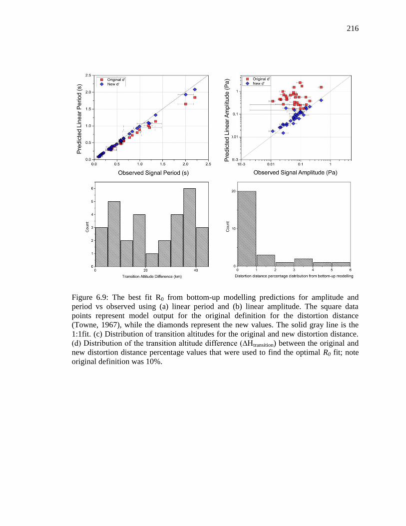
215

It was possible to find the converging amplitude-period solution in the linear

regime for the majority of arrivals (22/24). Three fits are as much as 20% beyond

the measurement uncertainty bounds for amplitude, while all others are within the

measurement uncertainty bounds for both period and amplitude.

When varying the constant in equation (6.18), the resultant distortion distance

percentage is well below 6%. The distribution is shown in Figure 6.9(d).

Moreover, it is not possible to define a set percentage that would be applicable to

all events. Some of these values may in fact not be realistic or feasible - we are

assuming that the entire cause of the difference in the linear amplitude vs. period

is due to the definition of the distortion distance, an assumption probably not fully

correct.

Smaller distortion distance leads to lower transition altitudes (Table 6.4). Half of

the arrivals (12/24) had their transition height below 5 km. The maximum

transition altitude was 25 km, with the mean altitude of 9 km; this means that no

weak shock wave can be approximated as transitioning to a linear acoustic wave

prior to reaching this height within the context of the original ReVelle (1974)

model and still produce physically reasonable amplitude estimates. With the

original definition for d’, the transition altitudes for our data were as high as 56

km, with a mean of 33 km. Cotten et al. (1971) examined propagation of shock

waves generated by Apollo rockets and noted that a wave would not be expected

to be acoustic above the altitude of 35-40 km at the large blast radii characteristic

of those vehicles.

Regardless of the extent of adjustment to the distortion distance, within the

context of the ReVelle (1974) model, self-consistent amplitudes and periods are

not possible unless some weak shock waves are assumed to never transition to

linear waves. – i.e. even using a 0% distortion in our data set, two arrivals had no

transition at all. However, these two arrivals also had a poor fit overall for any

distortion distance.

The lower transition altitude also implies that the difference between the classical

and Sutherland and Bass (2004) absorption coefficients is negligible in the

frequency range of our events.

216

Figure 6.9: The best fit R0 from bottom-up modelling predictions for amplitude and

period vs observed using (a) linear period and (b) linear amplitude. The square data

points represent model output for the original definition for the distortion distance

(Towne, 1967), while the diamonds represent the new values. The solid gray line is the

1:1fit. (c) Distribution of transition altitudes for the original and new distortion distance.

(d) Distribution of the transition altitude difference (∆Htransition) between the original and

new distortion distance percentage values that were used to find the optimal R0 fit; note

original definition was 10%.

217

Table 6.4: A summary of R0 as derived from the FM model. The associated outputs from

top-down modelling are also shown. The two entries in the Taltitude, which is the

transition height, in the “New d′” section denote events that never transition to the linear

regime. Therefore, the original definition for d’ was used by default.

We compared the infrasonic masses from the best fit R0 to the photometric masses

(Figure 6.10(a)) and found a much better agreement (on average to within order of

magnitude) than that resulting from the comparison between photometric and the

infrasonic masses from R0 using the original definition of distortion distance.

The mass from the FM model R0 should not exceed the mass used as the model input;

however, the contrary can be observed (Figure 6.10(b)). For a single spherical body and

no fragmentation and/or significant ablation, the blast radius can be estimated via

equation (6.2). However, if there is fragmentation and/or significant ablation, then the

Date Ro Ro err Tlin Tws Alin Aws Taltitude Tlin Tws Alin Aws Taltitude

20060419 1.09 0.05 0.09 0.09 0.234 0.119 10.0 0.09 0.09 0.125 0.119 1.1

20061104 2.45 0.01 0.17 0.19 0.216 0.031 25.4 0.18 0.19 0.048 0.031 7.1

20070125 25.95 0.36 1.05 1.26 1.363 0.021 55.0 1.22 1.26 0.053 0.021 12.8

20070727 11.48 0.21 0.68 0.80 0.731 0.04 38.4 0.79 0.80 0.054 0.04 5.0

20071021 66.66 5.36 2.24 2.65 2.202 0.036 54.5 2.53 2.65 0.148 0.036 19.3

20080325 5.79 0.39 0.32 0.35 0.639 0.195 16.1 0.33 0.35 0.452 0.195 12.0

20081028 2.52 0.22 0.15 0.16 0.582 0.272 10.9 0.16 0.16 0.317 0.272 2.6

20081102 5.30 0.55 0.36 0.40 0.23 0.017 33.2 0.38 0.40 0.091 0.017 22.2

20081107 0.56 0.43 0.06 0.06 0.044 0.006 25.8 0.06 0.06 0.007 0.006 1.3

20090523 1.99 0.36 0.17 0.19 0.167 0.022 26.5 0.18 0.19 0.094 0.022 19.5

20090917 4.68 0.47 0.33 0.36 0.39 0.047 27.8 0.35 0.36 0.105 0.047 11.9

20100421 15.88 0.07 0.85 0.96 0.587 0.036 36.2 0.95 0.96 0.044 0.036 3.5

20100429 8.87 0.79 0.53 0.61 0.387 0.015 42.5 0.59 0.61 0.037 0.015 12.7

20110520 9.97 0.20 0.56 0.65 0.439 0.015 42.0 0.63 0.65 0.038 0.015 11.9

20110630 7.42 0.05 0.46 0.53 0.392 0.018 40.6 0.53 0.53 0.021 0.018 2.4

20110808 12.32 0.06 0.62 0.68 0.9 0.254 17.2 0.62 0.68 0.9 0.254 17.2*

20111005 7.69 0.82 0.42 0.46 0.565 0.065 28.3 0.44 0.46 0.285 0.065 20.0

20111202 2.24 0.04 0.16 0.17 0.19 0.062 15.4 0.16 0.17 0.075 0.062 3.4

20060805 12.50 0.44 0.64 0.75 0.844 0.038 41.2 0.69 0.75 0.228 0.038 23.9

20060805 59.42 0.76 1.88 2.29 2.861 0.044 56.5 2.20 2.29 0.132 0.044 15.4

20080511 13.10 0.03 0.63 0.74 0.932 0.028 46.9 0.73 0.74 0.034 0.028 3.7

20080511 11.90 0.10 0.61 0.70 0.895 0.037 42.0 0.61 0.70 0.895 0.037 42.0*

20080812 5.75 0.19 0.38 0.43 0.326 0.02 37.0 0.43 0.43 0.021 0.02 1.4

20080812 6.34 0.15 0.40 0.46 0.348 0.018 39.1 0.46 0.46 0.02 0.018 2.2

20090428 5.11 1.08 0.31 0.33 0.486 0.171 14.6 0.32 0.33 0.306 0.171 8.7

20090428 2.28 0.01 0.18 0.19 0.165 0.037 20.2 0.19 0.19 0.043 0.037 2.8

20090812 0.76 0.08 0.08 0.09 0.05 0.007 26.7 0.09 0.09 0.008 0.007 2.6

20090812 0.75 0.07 0.08 0.09 0.049 0.007 26.6 0.09 0.09 0.011 0.007 7.6

20100530 3.35 0.13 0.26 0.31 0.198 0.008 41.8 0.30 0.31 0.014 0.008 7.7

20100530 3.29 0.14 0.26 0.30 0.196 0.009 41.1 0.30 0.30 0.011 0.009 3.6

Original d' [Towne, 1967] New d'

218

contributions from the particles/fragments falling off the main body may alter the blast

radius (Figure 6.11) such that there is an over-prediction of the meteoroid mass.

Figure 6.10: The comparison of the infrasonic and photometrically derived masses. (a)

Infrasonic mass from the best fit R0. The three points on the far left are from the two

events, which were poorly constrained in terms of the transition height and distortion

distance. The abscissa represents the equivalent photometric mass derived from the FM

model blast radius and equation (6.17); (b) The comparison between the FM model input

mass and the mass derived from the blast radius as per equation (6.17). The grey line is

the 1:1 line in all plots.

Figure 6.11: Blast radius produced by a single spherically shaped body. (b) Blast radius

produced during fragmentation or significant ablation.

219

Therefore, in such instances, the blast radius, while a good measure of energy deposition

by the meteoroid (R0 ~ (dE/dL)1/2

), is not a reliable means of obtaining the meteoroid

mass. Recall from section 6.1.2 that there are several crucial assumptions in the weak

shock model: (i) the meteoroid is a spherically shaped single body, (ii) there is no

fragmentation, and (iii) there is no significant deceleration and strong ablation. ReVelle

(2010) suggested that R0 from a fragmenting bolide may be as much as 5-20 times larger

(depending on height) than a non-fragmenting blast radius. Our study shows that strong

ablation is indeed an important effect, even for centimeter sized meteoroids. In fact, this

contribution is up to a factor of 10 and on average a factor of 3. Therefore, use of the R0 =

Mdm is not valid in most cases. The blast radius estimated from purely energy-based

(optical) considerations appears to be more robust.

Having done bottom-up and top down analysis, and blast radius and mass comparisons, it

is evident that without having some information about the source function (i.e.

measurements from video observations) the signal amplitude exhibits too much scatter to

be utilized in empirical blast radius estimates. Although the dominant signal period may

undergo variations due to competing processes of distortion and dispersion (ReVelle,

1974), this study demonstrates that the dominant signal period is much closer to ‘true’

values of R0 (e.g. Figures 6.5 and 6.6(a)).

In Figure 6.12 we show best fit R0 derived through the bottom-up modelling. For the

centimeter-sized meteoroids we may estimate an empirical period-R0 relation for the blast

radius from these bottom-up values. We have divided the final fits into two distinct blast

radius prediction populations: the short period (τobs ≤ 0.7s) and the long period (τobs >

0.7s) based on the source altitudes. The short period population, predicting R0 ≤ 10 m, is

confined to the shock source altitudes between 53 km and 95 km. The long period

population, predicting R0 > 10 m, is associated with the shock source altitudes extending

above 85 km. For short period population, the bottom-up based blast radius can be

estimated within 1.5 meters, and for long periods within ~5 m, although the number

statistics for the latter is small. We suspect much of the uncertainty at larger periods

reflects the greater role fragmentation may play for larger meteoroids. The overlap

altitude (85 – 95 km) between these two populations occurs at the mesopause and near

220

the transitional slip-flow regime for meteoroids ~1 centimetre in diameter (Campbell-

Brown and Koschny, 2004), suggesting that the weak shock model may not be correctly

predicting R0 in the free molecular flow regime.

For completeness, we also fitted the R0 calculated from the FM model. Recall that the FM

based R0 is derived from the energy deposition determined by fitting optical

measurements to the entry model. The FM based R0 has much more scatter, thus resulting

in the blast radius estimate uncertainty of up to 17 m.

The empirical relations for the blast radius derived from the bottom-up approach are:

R0 = 15.4231 τ – 0.5294 (τobs ≤ 0.7s) (6.19a)

R0 = 29.14597 τ – 11.5811 (τobs > 0.7s) (6.19b)

Even though there are a number of simplifications and assumptions in the weak shock

model, in its new modified form it offers a reasonable initial estimate for the blast radius

as a function of observed signal period, and therefore energy deposition for small

regional meteoroids, without making any assumptions about the fragmentation process.

Consequently, this methodology could be extended to high altitude explosive sources in

the atmosphere. The applicability of the weak shock model can also be further

investigated and extended to spherical shocks, especially if observational data can be

used in a similar fashion as in this study.

221

Figure 6.12: Blast radius from best fit bottom-up modelling versus observed signal for (a)

the short signal period (τobs ≤ 0.7 s) and (b) the long signal period (τobs > 0.7 s)

populations. Hs is the shock source height as derived from raytracing (Silber and Brown,

2014).

222

6.4 Conclusions

In this paper we extend the study of Silber and Brown (2014, in review) to critically

investigate the analytic blast wave model of the nonlinear disturbance initiated by an

explosive line source as an analog for a meteor shock as developed by ReVelle (1974).

We applied the updated ReVelle (1974) model to 24 of the best constrained

simultaneously optical and infrasound detected regional meteors to critically examine the

weak shock model. Here we summarize our main conclusions:

i. We analyzed the weak shock model behavior using a synthetic meteor, and

performed the sensitivity analysis on a set of meteor events from our data set to

examine the effect of the winds, perturbed wind fields due to gravity waves, and

Doppler shift. The overall effect of these factors on the initial value of the blast

radius is relatively small (<10%) for regional meteor events.

ii. We performed bottom-up modelling using the ReVelle (1974; 1976) approach to

determine the blast radius required to predict both the signal amplitude and period

at the ground such that it matches that observed by the receiver within

uncertainty. While the period-based R0 appears to have realistic values, the

amplitude-based R0 exhibits large systematic deviations in the linear and weak

shock regimes, as well as large deviations when compared to the period-based

blast radius. The amplitude-based R0 estimate severely under-predicts the

observed amplitude in the linear regime, and overestimates it in the weak shock

regime.

iii. Drawing upon the results from (ii), we varied the distortion distance to examine

its effect on the weak shock to linear transition altitude. We empirically

established that to match the observed amplitude of the meteor infrasound at the

ground within the context of the ReVelle (1974) model, the distortion distance for

our dataset must always be less than six percent, contrary to the proposed fixed 10

percent (Towne, 1967). The choice of definition of the distortion distance has a

strong effect on the predicted linear amplitude. We established the ‘best fit’ linear

regime R0 which matched both amplitude and period within their respective

measurement uncertainties. No one definition of modified distortion distance

223

worked for all events, but we found acceptable fits when the distortion distance

was assumed to be of an order half or less than the original ReVelle (1974)

adopted value.

iv. We applied the FM entry model (Ceplecha and ReVelle, 2005) to photometric

data as measured from video observations of meteor events to independently

calculate the blast radius using the fundamental definition for R0 in terms of

energy deposition per path length derived from the FM model. This blast radius

was used as an input for top-down modelling to determine the predicted signal

amplitude and period in both weak shock and linear regimes. Both the predicted

period and amplitude as obtained from the best fit R0 are nearly 1:1. This validates

the basic definition of blast radius and its fundamental linkage to energy

deposition during the hypervelocity meteor entry.

v. The infrasonic mass estimate is systematically larger than the mass estimated

from FM modeling and is not a reliable predictor of the true meteoroid mass using

any set of assumptions which we interpret as being mainly due to the ubiquitous

presence of fragmentation during ablation of centimeter-sized meteoroids. The

fragmentation tends to artificially increase the equivalent single-body mass,

making infrasonically determined mass less reliable for larger events.

vi. We derived new empirical relations which link the observed dominant signal

period to the meteoroid blast radius: R0 = 15.4231 τ – 0.5294 (τobs ≤ 0.7s) and R0 =

29.14597 τ – 11.5811 (τobs > 0.7s). The blast radius can be estimated to within 15

percent.

Even though the premise of the ReVelle (1974) weak shock model is to require some

knowledge about the source a priori to be able to predict the signal amplitude and the

period at receiver located at the ground, we have obtained an empirical relation which

can be used to estimate the source blast radius for centimeter-sized bright fireballs,

regardless of the meteoroid’s velocity, entry angle and other parameters which are

generally difficult to determine without video observations. In conclusion, the weak

shock model of meteor infrasound production (ReVelle, 1974) in its analytical form

offers a good first order estimate in determining the blast radius and therefore energy

224

deposition by small meteoroids, particularly if period alone is used or if no fragmentation

is present.

Acknowledgements

The authors would like to thank: J. Borovička, P Spurny and Z. Ceplecha for kindly

providing trajectory solution software and the FM model code. EAS thanks: CTBTO

Young Scientist Award (through European Union Council Decision 2010/461/CFSP IV)

for funding part of this project; L. Sutherland for generously providing worked out

atmospheric absorption coefficients; R. Weryk for assistance with the synthetic

photometry and all-sky camera development; J. Gill for setting up the parallel processing

machine; the British Atmospheric Data Centre for providing UKMO Assimilated

atmospheric data set. PGB thanks the Natural Sciences and Engineering Research

Council of Canada, the Canada Research Program and NASA cooperative agreement

NNX11AB76A for funding this work.

225

References

Andrews, D. G. (2010) An introduction to atmospheric physics. Cambridge University

Press, ISBN: 0521693187.

Arrowsmith, S. J., ReVelle, D., Edwards, W., & Brown, P. (2008) Global detection of

infrasonic signals from three large bolides. Earth, Moon, and Planets, 102(1-4),

357-363, doi: 10.1007/978-0-387-78419-9_50.

Baggaley, W. J. (2002) Radar observations, in: Murad, E., and Williams, I. P. (Eds.)

Meteors in the Earth's Atmosphere: Meteoroids and Cosmic Dust and Their

Interactions with the Earth's Upper Atmosphere, Cambridge University Press,

123–148, doi: 10.1029/1999JA900383.

Bedard, A., Georges, T. (2000) Atmospheric infrasound, Acoustics Australia, 28(2), 47-

52, doi: 10.1063/1.883019.

Boyd, I. D. (1998) Computation of atmospheric entry flow about a Leonid meteoroid.

Earth, Moon, and Planets, 82, 93-108, doi: 10.1023/A:1017042404484.

Bronsthen, V.A. (1983) Physics of Meteoric Phenomena, 372 pp., D. Reidel, Dordrecht,

Netherlands, ISBN: 978-94-009-7222-3.

Brown, P. G., Assink, J. D., Astiz, L., Blaauw, R., Boslough, M. B., Borovička, J., and 26

co-authors (2013) A 500-kiloton airburst over Chelyabinsk and an enhanced

hazard from small impactors, Nature, 503, 238-241, doi: 10.1038/nature12741.

Brown, P., ReVelle, D. O., Silber, E. A., Edwards, W. N., Arrowsmith, S., Jackson, L.

E.,Tancredi, G., Eaton, D. (2008) Analysis of a crater‐forming meteorite impact in

Peru. Journal of Geophysical Research: Planets (1991–2012), 113(E9), doi:

10.1029/2008JE003105.

Brown, P.G., Edwards, W.N., ReVelle, D.O., Spurny, P. (2007) Acoustic analysis of

shock production by very high-altitude meteors – I: infrasonic observations,

dynamics and luminosity, Journal of Atmospheric and Solar-Terrestrial Physics,

69: 600–620, doi: 10.1016/j.jastp.2006.10.011.

Burke, D. L., Axelrod, T., Blondin, S., Claver, C., Ivezić, Ž., Jones, L., Jones, L., Saha,

A., Smith, A., Smith, R. C., Stubbs, C. W. (2010) Precision determination of

atmospheric extinction at optical and near-infrared wavelengths. The

Astrophysical Journal, 720(1), 811, doi:10.1088/0004-637X/720/1/811.

Campbell-Brown, M. D., Koschny, D. (2004) Model of the ablation of faint meteors.

Astronomy and Astrophysics-Berlin Then Les Ulis, 418(2), 751-758, doi:

10.1051/0004-6361:20041001-1.

226

Carlson, H. W., Maglieri, D. J. (1972) Review of Sonic‐Boom Generation Theory and

Prediction Methods, The Journal of the Acoustical Society of America, 51, 675,

doi: 10.1121/1.1912901.

Ceplecha, Z., and R. E. McCrosky. (1976) Fireball end heights: A diagnostic for the

structure of meteoric material. Journal of Geophysical Research, 81(35), 6257-

6275, doi: 10.1029/JB081i035p06257.

Ceplecha, Z., and Revelle, D. O. (2005) Fragmentation model of meteoroid motion, mass

loss, and radiation in the atmosphere, Meteoritics & Planetary Science, 40(1), 35-

54, doi: 10.1111/j.1945-5100.2005.tb00363.x.

Ceplecha, Z., Borovička, J., Elford, W. G., ReVelle, D. O., Hawkes, R. L., Porubčan, V.,

and Šimek, M. (1998) Meteor phenomena and bodies, Space Science Reviews,

84(3-4), 327-471, doi: 10.1023/A:1005069928850.

Christie, D. R. Campus, P. (2010) The IMS Infrasound Network: Design and

Establishment of Infrasound Stations, In: A. Le Pichon, E. Blanc and A.

Hauchecorne, Eds., Infrasound Monitoring for Atmospheric Studies, Springer,

New York, pp. 29-75, doi: 10.1007/978-1-4020-9508-5_2.

Chyba, C. F., Thomas, P. J., Zahnle, K. J. (1993) The 1908 Tunguska explosion:

atmospheric disruption of a stony asteroid. Nature, 361(6407), 40-44, doi:

10.1038/361040a0.

Cook, R.K. and A.J. Bedard Jr (1972) On the measurement of Infrasound, Q. J. Roy.

Astro. Soc. 67, pp 5-11, doi: 10.1038/361040a0.

Cotten, D. E., Donn, W. L., and Oppenheim, A. (1971) On the generation and

propagation of shock waves from Apollo rockets at orbital altitudes, Geophysical

Journal of the Royal Astronomical Society, 26(1‐4), 149-159, doi:

10.1111/j.1365-246X.1971.tb03388.x.

DuMond, J. W., Cohen, E. R., Panofsky, W. K. H., Deeds, E. (1946). A determination of

the wave forms and laws of propagation and dissipation of ballistic shock waves.

The Journal of the Acoustical Society of America. 18, 97, doi:

10.1121/1.1916347.

Edwards, W. N. (2010) Meteor generated infrasound: theory and observation. In

Infrasound monitoring for atmospheric studies (pp. 361-414). Springer

Netherlands, doi: 10.1007/978-1-4020-9508-5_12

Edwards, W. N., Brown, P. G., Weryk, R. J., ReVelle, D. O. (2008) Infrasonic

observations of meteoroids: Preliminary results from a coordinated optical-radar-

infrasound observing campaign, Earth, Moon, and Planets. 102(1-4), 221-229,

doi: 10.1007/s11038-007-9154-6.

227

Ens, T. A., Brown, P. G., Edwards, W. N., Silber, E. A. (2012) Infrasound production by

bolides: A global statistical study, Journal of Atmospheric and Solar-Terrestrial

Physics, 80, 208-229, doi: 10.1016/j.jastp.2012.01.018.

Evans, L. B., Sutherland, L. C. (1971) Absorption of Sound in Air. The Journal of the

Acoustical Society of America, 49(1A), 110-110, doi: 10.1121/1.1975615.

Evers, L.G. H.W. Haak. (2001) Listening to sounds from an exploding meteor and

oceanic waves, Geophysical Research Letters, 30: 41-44, doi:

10.1029/2000GL011859.

Few, A. A. (1969) Power spectrum of thunder, J. Geophys. Res., 74, 6926-6934, doi:

10.1029/JC074i028p06926.

Garcés, M., Le Pichon, A. (2009) Infrasound from Earthquakes, Tsunamis and

Volcanoes, In: R. A. Meyers, Ed., Encyclopedia of Complexity and Systems

Science, Springer, Berlin, pp. 663-679, doi: 10.1007/978-0-387-30440-3_286.

Hawkes R. L. (2002) Detection and analysis procedures for visual, photographic and

image intensified CCD meteor observations. In Meteors in the Earth’s

Atmosphere, edited by Murad E., and Williams I. Cambridge Univ Press, pp. 97–

122, ISBN: 0521804310.

Haynes, C. P., Millet, C. (2013) A sensitivity analysis of meteoric infrasound, Journal of

Geophysical Research: Planets, 118(10), 2073-2082, doi: 10.1002/jgre.20116.

Hedlin, M.A., Garcés, M., Bass, H., Hayward, C., Herrin, G., Olson, J., Wilson, C.

(2002) Listening to the secret sounds of earth’s atmosphere, Eos 83, 557, 564-

565, doi: 10.1029/2002EO000383.

Hunt, J. N., Palmer, R., and Penney, W. (1960) Atmospheric waves caused by large

explosions. Philosophical Transactions of the Royal Society of London, Series A,

Mathematical and Physical Sciences, 252(1011), 275-315, doi:

10.1098/rsta.1960.0007.

Jacchia, L., Verniani, F., and Briggs, R. E. (1967) An analysis of the atmospheric

trajectories of 413 precisely reduced photographic meteors, Smithsonian

Contributions to Astrophysics, 10, 1-139.

Jones, D. L., Goyer, G. G., Plooster, M. N. (1968) Shock wave from a lightning

discharge. J Geophys Res, 73, 3121–3127, doi: 10.1029/JB073i010p03121.

Kraemer, D.R. (1977) Infrasound from accurately measured meteor trails, Ph.D. Thesis

Michigan Univ., Ann Arbor, MI, USA.

Kulichkov, S. N. (2004) Long-range propagation and scattering of low-frequency sound

pulses in the middle atmosphere, Meteorology and Atmospheric Physics, 85(1-3),

47-60, doi: 10.1007/s00703-003-0033-z.

228

Levison, H. F. (1996) Comet taxonomy, in Completing the Inventory of the Solar

System, Astronomical Society of the Pacific Conference Proceedings, T.W. Rettig

and J.M. Hahn, Eds., Vol. 107, pp. 173-191.

Lin, S. C. (1954) Cylindrical shock waves produced by instantaneous energy release, J

Appl Phys, 25, 54–57, doi: 10.1063/1.1721520.

Maglieri, D. J., Plotkin, K. J. (1991) Sonic boom, In Aeroacoustics of Flight Vehicles:

Theory and Practice, Volume 1: Noise Sources, Vol. 1, pp. 519-561

McKinley, D. W. R. (1961) Meteor Science and Engineering, McGraw-Hill Inc., New

York, NY, USA

Morse P. M., Ingard K. U. (1968) Theoretical Acoustics, McGraw-Hill, New York,

ISBN: 0691024014.

Mutschlecner, J. P., Whitaker, R. W. (2010) Some atmospheric effects on infrasound

signal amplitudes. In Infrasound Monitoring for Atmospheric Studies, pp. 455-

474, Springer Netherlands, doi: 10.1007/978-1-4020-9508-5_14.

Officer, C. B. (1958) Introduction to the theory of sound transmission: With application

to the ocean, pp. 284, New York: McGraw-Hill, USA.

Ostashev, V. (2002) Acoustics in moving inhomogeneous media, CRC Press, USA,

ISBN: 0419224300.

Pichon, A. L., Antier, K., Cansi, Y., Hernandez, B., Minaya, E., Burgoa, B., ... &

Vaubaillon, J. (2008) Evidence for a meteoritic origin of the September 15, 2007,

Carancas crater. Meteoritics & Planetary Science, 43(11), 1797-1809, doi:

10.1111/j.1945-5100.2008.tb00644.x.

Pierce, A. D., Thomas, C. (1969) Atmospheric correction factor for sonic-boom pressure

amplitudes, Journal of the Acoustical Society of America, 46, 1366-1380, doi:

10.1121/1.1911861.

Plooster, M. N. (1970) Shock waves from line sources, Numerical solutions and

experimental measurements, Physics of fluids, 13, 2665, doi: 10.1063/1.1692848.

Plotkin, K. (1989) Review of sonic boom theory, AAIA 12th Aeronautics Conference,

April 10-12, 1989, San Antonio, TX, USA

Popova, O. P., Jenniskens, P., Emel’yanenko, V., Kartashova, A., Biryukov, E.,

Khaibrakhmanov, S., et al. (2013) Chelyabinsk Airburst, Damage Assessment,

Meteorite Recovery, and Characterization. Science, 342(6162), 1069-1073, doi:

10.1126/science.1242642.

ReVelle, D. O. (1974) Acoustics of meteors-effects of the atmospheric temperature and

wind structure on the sounds produced by meteors. Ph.D. Thesis Michigan Univ.,

Ann Arbor MI, USA.

229

ReVelle, D. O. (1976) On meteor‐generated infrasound, Journal of Geophysical

Research, 81(7), 1217-1230, doi: 10.1029/JA081i007p01217.

ReVelle, D. O. (1997) Historical Detection of Atmospheric Impacts by Large Bolides

Using Acoustic-Gravity Waves, Ann N Y Acad Sci, 822 (1 near-earth ob), 284,

doi: 10.1111/j.1749-6632.1997.tb48347.x.

ReVelle, D. O. (2010) Acoustic-gravity waves from impulsive sources in the atmosphere,

In Infrasound Monitoring for Atmospheric Studies, pp. 305-359, Springer

Netherlands, doi: 10.1007/978-1-4020-9508-5_11.

Sakurai, A. (1964) Blast Wave Theory, Report No. MRC-TSR-497, Wisconsin Univ-

Madison Mathematics Research Center, USA.

Silber, E. A., Brown, P. G. (2014) Optical Observations of Meteors Generating

Infrasound – I: Acoustic Signal Identification and Phenomenology, JASTP,

submitted (#ATP3766)

Silber, E. A., Le Pichon, A. Brown, P. (2011) Infrasonic Detection of a Near-Earth

Object Impact over Indonesia on 8 October, 2009, Geophysical Research Letters,

Vol. 38, L12201, doi: 10.1029/2011GL047633.

Silber, E. A., ReVelle, D. O., Brown, P. G., Edwards, W. N. (2009) An estimate of the

terrestrial influx of large meteoroids from infrasonic measurements, Journal of

Geophysical Research: Planets (1991–2012), 114(E8), doi:

10.1029/2009JE003334.

Sutherland, L. C., Bass, H. E. (2004) Atmospheric absorption in the atmosphere up to

160 km. The Journal of the Acoustical Society of America, 115, 1012, doi:

10.1121/1.1631937.

Swift, W. R., Suggs, R. M., and Cooke, W. J. (2004) Meteor44 video meteor photometry,

Earth, Moon, and Planets, 95(1-4), 533-540, doi: 10.1007/1-4020-5075-5_49.

Towne, D.H. (1967) Wave Phenomena, Addison-Wesley Publications, Reading,

Massachusetts, USA

Tsikulin, M. A. (1970) Shock waves during the movement of large meteorites in the

atmosphere, Report No. NIC-Trans-3148, Naval Intelligence Command

Alexandria, VA Translation Div., USA

Vargas, M. J., Benítez, P. M., Bajo, F. S., Vivas, A. A. (2002) Measurements of

atmospheric extinction at a ground level observatory, Astrophysics and space

science, 279(3), 261-269, doi: 10.1023/A:1015184127925

Wallace, J. M. and Hobbs, P.V. (2006) Atmospheric Science: An Introductory Survey,

Academic Press, 2nd edition, ISBN: 012732951X.

230

Weryk, R. J., and Brown, P. G. (2013) Simultaneous radar and video meteors—II:

Photometry and ionisation. Planetary and Space Science, 81, 32-47, doi:

10.1016/j.pss.2011.12.023.

Whitham, G. B. (1952) The flow pattern of a supersonic projectile. Communications on

pure and applied mathematics. 5(3), 301-348, doi: 10.1002/cpa.3160050305.