chapter 5. rf wireless communications 5.4 data rate ...mason.gmu.edu/~rmorika2/chapter 5 riki v4...

Fundamentals of Telecommunications and Networking for IT R.Morikawa

1

Chapter 5. RF Wireless Communications 5.1 Introduction 5.2 Antennas Basics 5.2.1 Electromagnetic (EM) wave and Antenna Polarization 5.2.2 Antenna Gain 5.3 Link Analysis

5.3.1 Link Analysis - Determining Carrier-to-Noise (CNR) 5.3.1.1 Noise Factor and Noise Figure 5.3.2 G/T, Receive System Figure-of-Merit 5.4 Data Rate Capacity 5.5 Multipath and MIMO 5.6 Spread Spectrum 5.6.1 A Closer Look at DSSS 5.7 Orthogonal Frequency Division Multiplexing (OFDM) Key Terms Chapter 5 Problems


2

Chapter 5. RF Wireless Communications

"I do not think that the radio waves I have discovered will have any practical application." Heinrich Hertz (http://www.azquotes.com/author/22801-Heinrich_Hertz)

5.1 Introduction

While optical fibers provide the high capacity communications needed for today's multimedia environment, wireless communications give us mobility free from wired connections that is highly desirable to many of us. In fact our demand for mobile communications have increased dramatically. Unfortunately, wireless communications is limited by the availability of useable frequency spectrum over a shared free space environment, as well as the susceptibility to electromagnetic interference (EMI) from multiple sources both natural and man-made. In response to satisfying ever increasing user demands for high capacity mobile communications, engineers have developed new technologies and methods that have increased the efficiency of how we use the limited frequency spectrum that is available. Through these innovative efforts, today's wireless systems offer high capacity multimedia to many users in many different forms such as text, images, voice and video.

The technical innovations used in wireless communications today typically involves the application of processors that enable engineers to develop advanced and complex digital signal processing and modulation techniques, as well as sophisticated antenna systems. In this chapter, we go over the basic principles of antennas and the unique issues presented by multipath propagation of RF signals. We introduce link analysis, which is a methodology in which we determine receive power based upon transmit power, signal attenuation or link losses, and antenna gain. In addition we will discuss spread spectrum and orthogonal frequency division multiplexing (OFDM) techniques, and how these can be applied to increase resistance to RF interference (RFI).

5.2 Antenna Basics

In chapter 1, we discussed how a current traveling through a conductive wire creates an electromagnetic (EM) wave that surrounds the wire. By using an antenna, the EM wave produced by the current flow can be transformed into an EM wave that can propagate through free space. When designing an antenna for maximum signal power and efficiency, engineers will ensure that the antenna is resonant at the transmission frequency. Resonance occurs when the reactive1 components of the antenna cancel one another out, leaving just the desirable resistive component that maximizes the RF power. Non-resonant antennas are also used for communications although they are not as sensitive or efficient as their resonant counterparts. Therefore, when using non-resonant antennas, receivers with greater sensitivity are typically required. Non-resonant antennas also have a wider frequency bandwidth in

1 Recall from chapter 1 that reactance consists of both inductive and capacitive components.


3

comparison to resonant antennas that operate within a narrow bandwidth near resonant frequency.

The physical dimensions of an antenna are closely related to the wavelength of the signal. As an example, a basic dipole antenna shown in figure 5.1, has an antenna length that is one half of the transmission wavelength. Knowing the relationship between wavelength and frequency

(i.e., f=c/), we see that a wavelength of /2 equates to the second harmonic of the transmission frequency. In other words, antenna length matching the transmission fundamental frequency or its harmonic component, will ensure resonance and transmission efficiency (i.e., efficient transfer of RF power from the antenna). The Antenna Reciprocity Theorem further states that an antenna's RF properties will be identical whether it is transmitting or receiving. So the same antenna efficiency achieved while transmitting a signal, will be the same efficiency realized when receiving that same signal. We will see later on that this theory applies to all antenna characteristics including antenna gain and beamwidth.

Figure 5.1. Half-wave dipole antenna is a simple antenna with a length of /2. In the half-wave dipole, the signal conductor is connected to the middle of the antenna system.

For antenna length, we could have selected a full wavelength (i.e., fundamental frequency vice a harmonic), however, depending upon the transmission frequency, this could lead to very long antennas that might be unacceptable for most application. As an example, if we design a simple vertical full-wave antenna that resonates at 50 MHz, then the antenna length would be equal to the transmission wavelength, or:

= 𝑐

𝑓 = 3E8 (m/s) 50E6 Hz = 6 meters

Of course, using a 6 meter length antenna may be impractical for many situations. Since we know that resonance will occur at fractions of the fundamental wavelength, we can design an

antenna with a much shorter length. As an example, we could have used ½, or even ¼, which would have reduced the length of our antenna significantly.

Ant. Length = 𝑐

2𝑓 = 3E8 (m/s)100E6(Hz) = 3 meters (half-wave (/2))


4

Ant. Length = 𝑐

4𝑓 = 3E8 (m/s)200E6(Hz) = 1.5 meters (quarter-wave (/4))

When connecting an antenna to the signal cable, it is important to match the impedance of the cable to the impedance of the antenna. Impedance is comprised of both resistive and reactive components shown in equation (5.1), where Z is impedance, R is the resistive and X the reactive components. (Note: jX, termed the imaginary reactive component of impedance where j=(-1)1/2. The term jX gives us the phase angle information between signal voltage and current.)

Impedance, Z = R + jX (5.1)

An electrical current flowing in a single direction (i.e., DC, direct current) has an impedance that is purely resistive, and therefore Z=R. However, electrical signals that carry information will have varying current direction and voltage, thus giving rise to the additional reactive components of capacitance and inductance. The resulting impedance characterizes the cable and antenna, and must be identical in value to prevent destructive signal reflections. By matching impedance we ensure maximum power transfer across the interface. While impedance values used to today vary, two common values used for RF communications is 50Ω and 75Ω (ohms).

Antennas are designed to radiate transmitted power in different patterns depending upon purpose. As an example, broadcast antennas need to radiate over large areas in all directions, while microwave antennas are designed to radiate in a single direction. Directionality describes the direction relative to the antenna where the highest transmit or receive power is found. As an example, a microwave antenna is highly directional because it maximizes power in a direction towards the receive antenna. Associated with directionality is antenna gain, which describes the increase in power density (watts/m2) of a directional antenna when compared to an ideal isotropic antenna transmitting at the same power. To illustrate the concept of antenna gain, recall from chapter 1 that an ideal isotropic is a theoretical antenna where transmit power radiates from a point and spreads in a spherical pattern over time (figure 5.2a). Since the transmit power spreads outwardly over the surface area of the increasing sphere, the power density in watts per area decreases significantly. However, if we direct the power from the antenna towards certain desired directions, then we reduce attenuation and maintain higher power density in those directions. The half-wave dipole antenna in fig. 5.2b shows that maximum power radiation is concentrated around the sides of the antenna in a toriod or donut pattern. Since transmit power does not propagate in the areas above and below the dipole, more power density is available to propagate around the sides in a 360 degree pattern, thus higher power density is found in this area when compared to the isotropic antenna. The directionality of the dipole provides a gain of power density when compared to the isotopic antenna, and we typically use decibels to represent this gain. Eq. 5.2 shows antenna gain in decibels as a comparison of the power density (PD) of a half-wave dipole relative to the PD of the ideal isotropic antenna. We use dBi to show that the antenna's gain is relative to that of the isotropic case. In this equation, we can replace the half-wave pole PD with any other type of directional antenna in order to determine antenna gain in dBi.

Antenna Gain, G(dBi) = 10log10(PDhalf-dipole/PDisotopric) (5.2)


5

Figure 5.2. Antenna propagation. (a) An ideal isotropic antenna is a theoretical antenna that propagates in a perfect spherical pattern from a single point. (b) Drawing shows a cross

section of the propagation pattern for a half-dipole antenna. The shape of propagation is the shape of a toroid where signal nulls appear at the ends of the antenna.

Antennas are designed to provide specific radiation patterns in order to meet particular applications. The Antenna Reciprocity Theorem tells us that the radiation pattern of an antenna is the same whether in transmit or receive mode. The design of the antenna also determines the EM polarity of the signal being transmitted and received. The next section discusses EM and antenna polarization.

5.2.1 Electromagnetic (EM) wave and Antenna Polarization

EM polarization is defined by the direction of the electric field. In fig. 5.3, the electric field (E-field) is parallel to the y-axis and therefore the EM wave is considered vertically polarized. The magnetic field (H-field), which lies along the x-axis, mirrors the E-field and is always perpendicular to it. Had the E-field been parallel to the x-axis instead, the EM wave would have been considered horizontally polarized with the magnetic field perpendicular along the y-axis. For terrestrial, communications, vertical antennas are perpendicular to the earth's surface and they produce vertically polarized EM waves. Horizontal antennas are parallel to the earth's surface and produce horizontally polarized EM waves.

An EM wave can also be circularly polarized where the E-field rotates in either a clockwise or counterclockwise manner. The rotation of a Right Hand Circular Polarized (RHCP) EM wave can be determined using the "right hand rule" where the thumb of the right hand points in the direction of propagation, and the fingers curl towards the rotation of the wave. In this case, RHCP waves appear to rotate in a clockwise direction when viewed from the antenna along the line of propagation. Likewise, the rotation of Left Hand Circular Polarized (LHCP) waves can be


6

determined using the "left hand rule" in which the EM wave appears to rotate in a counterclockwise direction when viewed from the antenna along the propagation path.

A circularly polarized wave can be produced by simultaneously transmitting the same signal on both the vertical and horizontal planes, but with one of the signals shifted by a phase angle of 90 degrees or π/2 radians. By shifting the phase of either Ey or Ex, the resultant E-field will rotate in either a clockwise or counterclockwise direction depending upon the direction of the phase shift itself.

In fig 5.4 we see that two identical signals create a resultant wave whose magnitude is |E|=(EY

2+EX2)1/2 at an angle of Ө=tan-1(EY/EX). In fig. 5.4(a), both EY and EX signals are in phase

and therefore the resultant wave lies within the same plane as EY and EX. In fig. 4.5(b), we change the phase angle of the signal on EY by +π/2 radians, to EY=|E|sin(2πft + π/2), and leave EX= |E|sin(2πft) unmodified2. The phase shift in EY causes the resultant wave to rotate in a counterclockwise direction (i.e., LHCP). We can similarly change the phase angle of either EY or EX to cause a rotation in the opposite direction (i.e., LHCP). In practice, a quarter wave plate, which is designed to shift a signal plane phase by 90 degrees, is one of the popular ways used to create circularly polarized waves.

Figure 5.3. EM Wave. The E-field (red wave) is vertically polarized along the Y axis. The M-field (black wave) is perpendicular and proportional to the E-field.

2 EY leads EX by π/2 radians.


7

Figure 5. 4. Circularly Polarized EM Wave. The propagation of the wave in (a) and (b) is outward from the page.

In order to maximize the power transfer between transmit and receive antennas, the polarization of both antennas must be identical. Any variation between the two reduces the power transferred between antennas. This is true for linear polarized antennas (i.e., vertical and horizontal), as well as circularly polarized antennas (i.e., LHCP and RHCP). If the polarization of the EM wave changes during propagation from transmit to receive antennas, it is called depolarization. The resulting misalignment between the EM wave and the receive antenna causes a weakening of the signal. The greater the misalignment, the weaker the received. There are several causes of depolarization such as ice, snow, or free electrons found in the ionosphere3.

To illustrate the concept of depolarization, consider a vertically polarized EM wave that is collected (i.e., received) by a vertically polarized antenna in figure 5.5. We will assume that EY is a unit value equal to 1. Fig 5.5(a) shows the case where no depolarization of the EM wave has been experienced during propagation from the transmitter and, therefore all of the energy is found within the EY plane. In this case maximum energy transfer4 occurs between the EM wave and the receive antenna. In fig. 5.5(b), the EM wave encounters depolarization elements during propagation to the receiver, which in turn causes the EM wave to shift by 30 degrees. This shift creates a resultant wave, |E|, that is comprised of a vertical copolar component, EY, and a horizontal cross-polar component, EX. The straight brackets around |E| indicates the

3 The ionosphere is the upper most layer of earth's atmosphere. Satellite communications are particularly affected

by this layer. 4 Note: For this particular example, we are not considering attenuation, but are instead focusing on the power

reduction cause by depolarization.


8

magnitude of the resultant wave, which in this case is |E|=1. This is the same value as EY in the non-depolarized case. By applying basic trigonometry, we can determine the values of the copolar and cross-polar components.

|E|=(EX2+EY

2)1/2 = 1 (5.3) EX=|E|sin(Ө) = |E|(0.5) = 0.5

EY=|E|cos(Ө) = |E|(0.866) = 0.866

From equations in (5.3), we find that the vertical (copolar) component has decreased from 1 in the non-depolarized case, to 0.866 in the depolarized case. This means that depolarization has decreased the power transferred to the vertical antenna by (1 - 0.86 = 0.14) 14%. In addition, a cross polar component along the EX plane has been created which could adversely impact signals operating in the horizontal plane.

Figure 5.5. Effect of signal depolarization.

As the depolarizing shift continues to increase, the signal power available to the receive vertical antenna decreases. At a maximum shift of 90 degrees, the EM wave becomes horizontally polarized, or orthogonal5 to the vertical polarization, and a loss of 30 dB is experienced. A 30dB loss essentially means that no power is received by the vertical antenna. Similarly, horizontal, LHCP and RHCP antennas are effected by depolarization, which causes decreased energy transfer.

However, in cases where frequency reuse is desired, signals that are on the same frequency but orthogonal to one another in polarization can be reused. This means that the simultaneous

5 Orthogonal means opposite or perpendicular to. As an example, vertical polarization is orthogonal to horizontal

polarization, and RHCP is orthogonal to LHCP.


9

transmission of two channels on the same frequency can be achieved when operating on orthogonal planes (i.e., horizontal and vertical, LHCP and RHCP), thus doubling the number of available channels. It should be noted, however, that depolarization in the case of frequency re-use is still problematic, since depolarization causes the formation of cross polarization components in the orthogonal plane, which in turn creates interference to the signal operating in that plane.

5.2.2 Antenna Gain

All realistic antennas have a radiation pattern where power density is greater in some directions than others. As an example, with the half-wave dipole antenna in figure 5.2(b) the greatest power density is found perpendicular to the antenna at the sides in a 360 degree pattern. The power density gradually decreases to zero towards the two tips of the antenna, making a three dimensional donut shaped radiation pattern. When we compare this to the radiation pattern of the ideal isotropic antenna at the same power level, we see that the half-wave dipole has more power density perpendicular to the antenna than the ideal isotropic antenna. As discussed previously, we can describe this antenna gain in decibels referenced to the isotropic case in dBi.

Antenna gain is described by several variables which include frequency, physical antenna dimensions, and antenna efficiency. We will illustrate these variables by considering the case of a highly directional parabolic reflector antenna. Parabolic reflector antennas are typically circular in shape, although other rectangular or elliptical shapes are often used. The common characteristic of parabolic antennas is its reflector shape which creates a focal point for the collection or transmission of RF energy. When in receive mode, the reflector collects signal power density and reflects it towards a receiver feed which is located at the focal point of the parabola. When in transmit mode, power emanates from the transmit feed at the focal point and is reflected by the parabolic reflector towards the desired transmission direction.

Figure 5.6 depicts front and side views of a typical parabolic antenna. The main circular reflector is shaped into a paraboloid with a focal point located in front. The larger the area of the antenna is, the more power density it can collect during reception, and the greater the antenna gain. Likewise, per the Antenna Reciprocity Theorem, the transmit characteristics of the antenna are the same as for reception, therefore transmit antenna gain also increases as the area of the antenna increases. The physical area of the main reflector is simply the area of a circle, APHY=πr2, where r is the radius. Since we know that the diameter of a circle is D=2r, we can substitute D for r, see eq. (5.4).

APHY = πr2 = 𝜋(𝐷

2)2 =

𝜋𝐷2

4 (5.4)

However, not all of the antenna's physical area is useful in capturing the power density of the signal. The effective aperture, Ae, of the antenna is the useful receiving cross section that

actually captures the power density of the signal. Therefore, antenna efficiency, , is the ratio

of Ae over APHY (see eq. (5.5)). For a parabolic antenna, can range from a low of 30% to a high of 70%. A typical value for parabolic antennas is 50%.


10

= Ae/APHY (5.5)

Figure 5.6. Parabolic Antenna.

Example 5.1: A three meter parabolic antenna has an antenna efficiency of =55%. What is the area of the effective aperture Ae?

Answer: By using equations (5.4) and 5.5):

APHY = 𝜋𝐷2

4 =

𝜋32

4 =

9𝜋

4 = 7.0686 m2

Ae = APHY = (0.55)(7.068 m2) = 3.8877 m2

The gain of a parabolic antenna is dependent upon the frequency of the signal, diameter of the

antenna, and antenna efficiency as seen in equation (5.6), where is the signal's wavelength6. By substituting eq. (5.4) into (5.6), we can derive a second equation(5.7) which has the antenna diameter, D, as a variable. Either eqs (5.6) or (5.7) can be used to determine antenna gain.

G = ( x APHY)(4𝜋

2 ) (5.6)

𝐺 = πD2

4

4π

2 =

π2D2

2 = (

πD

)2 (5.7)

Example 5.2: Given the effective antenna aperture in example 5.1, and an operating frequency of 14GHz, what is the gain of the antenna in decibels?

Answer: We first determine the wavelength of the operating frequency,

6 Frequency equals the speed of light in a vacuum divided by wavelength (f=c/ where c=3E8 m/s)


11

= 3E8 (m/s) 14E9 Hz = 0.0214 meters

Using eq. (5.6),

Ae = APHY = 3.8877 m2

G = ( x APHY)( 4𝜋

2 ) = (3.8877 m2)(4π/4.5796E-4 m2) = 106,678

[G](dBi) = 10 log10(106,678) = 50.28 dBi

Alternatively, we could have used eq. (5.7), shown below.

D = 3 m, =0.55

G = (πD

)2 = 0.55(3π/0.0214m)2 = 106,678

[G](dBi) = 10 log10(106,678) = 50.28 dBi

When an antenna transmits, the power that emanates from the antenna is termed the Effective Isotropic Radiated Power (EIRP) which is the power entering the antenna, P, combined with the gain of the antenna, G, (see eq. 5.8). This value is typically shown in decibel form referenced7 to 1 watt (dBW) or 1 milliwatt (dBm).

EIRP = P x G (5.8)

[EIRP]dBW = 10log10(P/1W) +10log10G (5.9)

[EIRP]dBm = 10log10(P/1mW) +10log10G (5.10)

5.3 Link Analysis

In any communications system, whether guided or unguided, our goal is to ensure that enough power reaches the receiver, so that the signal can be properly detected and demodulated. This requires an understanding of how much power is emitted by the transmit antenna (i.e., EIRP), the amount of path loss our signal may encounter during propagation, and how much power actually reaches the receiver itself. Each receiver will have a specification regarding receive sensitivity, which tells us the minimum signal level required for that particular receiver to properly detect the signal for demodulation. As such, receiver sensitivity will vary depending upon the manufacturer of the radio. Typically, receive sensitivity is given in values of minimum dBm that the receiver requires for signal detection. Determining the amount of receive power in our communications link by adding gains and subtracting losses is termed link analysis.

7 Other power references are used as well such as dBµW which is referenced to 1 micro-watt.


12

Figure 5.7. Simple microwave communications link.

Figure 5.7 shows a simple microwave communications link. We can perform link analysis using non-decibel or decibel values, although the later makes it mathematically simpler, especially if we must change loss or gain values often. Using either method, we set PR, the received power, to one side of the equation as seen in equation (5.11). On the other side we begin our analysis starting with PT, transmit power. PT is combined with the transmit antenna's gain, GT, resulting in EIRP=PTGT or in decibels, [EIRP]=[PT]+[GT]. As the signal propagates from the transmit antenna to the receive antenna the signal experiences attenuation due to signal spreading. This attenuation can be determined using the Friis Free Space Loss equation (5.13), which is

dependent upon transmission frequency, f=c/, and the distance between antennas, d, in meters. Finally, once the signal reaches the receive antenna, it is combined with the receive antenna's gain, GR.

𝑃𝑅 = 𝑃𝑇 𝐺𝑇 𝐺𝑅

𝐹𝑆𝐿=

𝐸𝐼𝑅𝑃 𝐺𝑅

𝐹𝑆𝐿 (5.11)

Link Analysis equation in decibel form, [PR] = [PT]+[GT]+[GR]-[FSL] = [EIRP]+[GR]-[FSL] (5.12)

Friis Free Space Loss equation,

𝐹𝑆𝐿 = (4πd

)2 (5.13)

FSL in decibel form,

[FSL](dB) = 20log10(4πd) - 20log10() (5.14)

In the non-decibel case, we can combine eqs. (5.11) and (5.13), which gives us the basic link analysis equation (5.15).

𝑃𝑅 = 𝑃𝑇 𝐺𝑇 𝐺𝑅

(4πd

)2

= 𝑃𝑇 𝐺𝑇 𝐺𝑅 2

(4πd)2 (5.15)


13

Using decibels, eqs. (5.12) and (5.14) are combined to give us equation (5.16).

[PR] = [EIRP]+[GR]-[FSL] = [EIRP]+[GR]-( 20log10(4πd) - 20log10()) (5.16)

Note: The FSL equation can be rearranged as below:

−𝐹𝑆𝐿 =

4𝜋𝑑

2

, which in decibel form gives you a negative value for FSL:

-[FSL] = 20log10() - 20log10(4πd)

Therefore, if using the above equation for FSL, you must add, vice subtract, FSL:

[PR] = [EIRP]+[GR]+[FSL] = [EIRP]+[GR]+( 20log10() - 20log10(4πd))

Example 5.3: Determine the Friis FSL in decibels between transmitting antennas that are spaced 35 kilometers from one another. The transmission frequency is 9 GHz.

Answer: First we determine the wavelength in meters as:

=c/f=(3E8 m/s)/(9E9Hz) = 0.034 meters

Applying eq. (5.13): Note that we convert both frequency and distance to basic units of Hertz and meters. Doing this ensures that we do not inadvertently introduce large errors into our solution.

𝐹𝑆𝐿 = (4πd

)2 = (

4π35E3 m

0.034 m)2 = 1.74𝐸14

In decibels: [FSL] = 10log10(1.74E14) = 142.41 dB

In all practical situations, there are other losses and gains that must be taken into consideration when determining the power at our receiver. The losses can come in the form of weather, signal obstacles such as a building or terrain feature, as well as signal gains from amplifiers or digital repeaters. Let's consider figure 5.8, where we've added signal amplifiers for gain, and coaxial runs which introduce attenuation losses.


14

Figure 5.8. Link Analysis of a microwave communications link where cable losses and signal amplifiers are part of the circuit.

We can analyze this link by breaking it into section. Starting at the transmitter, PT is amplified by Amp1. The amplified signal then suffers attenuation, L1, as it propagates through the coaxial cable up to the antenna. The resulting power P1 enters the transmit antenna and is combined with the transmit antenna gain GT, resulting in EIRP (eq. 5.13). The transmit antenna has a gain equal to GT, and therefore our EIRP = P1 x GT (eq.5.17). We can solve EIRP using decibel notation, which reduces our equation to simple addition and subtraction (eq. 5.18).

EIRP = P1 x GT = 𝑃𝑇∗𝐴𝑚𝑝 1∗𝐺𝑇

𝐿1 (5.17)

[EIRP] = [P1] + [GT] = [PT] + [Amp1] + [GT] - [L1] (5.18)

Example 5.4: Given the communications link shown in fig. 5.8, determine the EIRP in decibels given the following: PT = 10W, Amp1 multiplies the signal x10, L1 attenuates the signal by 2db per 100 meters, the coaxial cable length from Amp1 to the antenna is 55 meters, GT=41dB. Solution 1: Using the non-decibels, and eq. (5.17), [L1] = (2dB/100m) x 55 m = 2.2dB

or in non-decibel: L1 = 10(2.2/10)= 1.659

[GT]= 41 dBi, or in non-decibel form, GT = 10(41/10) = 12,589.254

P1 = (PT x Amp1)/L1 = (10W x 10)/1.659 = 60.277 watts

EIRP = P1 x GT = 60.277W x 12,589.254 = 758,842.463 watts

Solution 2: Using the decibels, and equations (5.18), [PT] = 10 log10(10W/1W) = 10dBW,


15

[L1] = (2dB/100m) x 55 m = 2.2dB,

[GT]= 41 dBi, [Amp1] = 10log10(10/1) = 10dB,

[P1]= [PT ] + [Amp1] - [L1] = 10dBW + 10dB - 2.2dB = 17.8dBW

[EIRP] = [P1] + [GT] = 17.8dBW + 41dBi = 58.8dBW

We can check to see if the two solutions are the same by converting solution 2 [EIRP] back to watts.

EIRP (Watts) = 10(58.5/10) = 758,577.57 Watts

(note: we see a slight difference in watts between solutions 1 and 2. This is due to rounding off errors. In this case, the two solutions, while slightly different, validates our use of either the non-decibel or decibel methods).

The next step in our link analysis is to determine the Friis Free Space Loss (FSL) between our transmit and receive antennas using eq. (5.13) or in decibels using eq. (5.14). By including FSL, we determine the amount of signal power density reaching the receive antenna. This signal power density (watts per m2) is captured by the receive antenna's effective aperture (Ae) cross sectional area in m2, resulting in a signal power in watts entering the receive system. The receive antenna's gain, GR, is applied to the receive signal resulting in signal power P2 in watts. As the signal propagates through the coaxial cable, it suffers a power loss due to attenuation of L2. Finally, the attenuated signal is amplified by Amp2, which results in PR. By converting all variables in our link to decibel values, we can use simple addition and subtraction to determine the power PR that we expect to see at the front of our receiver (see eq. 5.19).

[PR]= [EIRP] - [FSL] + [GR] - [L2] + [Amp2] (5.19) Where, [EIRP]= [PT] + [Amp1] - [L1] + [GT]

Example 5.5: Given the communications link shown in fig. 5.8, and the following information provided below, determine the received power, PR. Transmit system: PT = 10W, frequency 5GHz, Amp1 x10, L1= 2db, GT=41dBi. Receiver system: GR=47dBi, Amp1 x2, L2 attenuates 1.5db. Misc. information: distance between antennas is d = 68 kilometers

Solution: = 𝑐

𝑓 = (3E8 m/s)/5E9 Hz = 0.06 meters,

[EIRP](dBW)= [PT]+[Amp1]-[L1]+[GT] = 10log10(10W/1W) +10log1010 - 2dB + 41 dBi = 10dBW + 10dB -2dB + 41dBi = 59 dBW


16

[FSL](dB) = 20log10(4πd) - 20log10() = 20log10(4π68E3 m) - 20log10(0.06 m) = 118.64 - (-24.44) = 143 dB

[PR](dBW) = [EIRP]-[FSL]+[GR]-[L2]+[Amp2] = 59dBW-143dB+47dBi-1.5dB+10log10(2) = 59dBW-143dB+47dBi-1.5dB+3.01dB = -35.49dBW

Example 5.6: Given the PR calculated in example 5.5, and a receive sensitivity of -10dBm, will your link close - i.e., is there enough signal strength at the receiver to detect and demodulate the received signal PR?

Solution: Convert [PR] from dBW to dBm: -35.49dBW + 30 = -5.49dBm

Since the power reaching the receiver is greater than the receive sensitivity, the receiver is able to detect ad demodulate the signal. The link margin is therefore,

[Link Margin] = [PR] - [Receive sensitivity] = -5.49dBm - (-10dBm) = 4.51dBm

5.3.1 Link Analysis - Determining Carrier-to-Noise Ratio (CNR)

Now that we have determined the level of power at the receiver, PR, we need to consider the effects of noise, especially as it impacts our receive system. We do this by determining the noise contributors at the receiver which primarily include receive antenna and system noise.

Earlier we discussed the signal-to-noise ratio (SNR), which we associated with a detected and demodulated signal found at the receiver's output. However, for our link analysis, we are more concerned with the power, PR, at the input of the receiver, which we call the Carrier-to-Noise Ratio (CNR). CNR represents PR measured over the noise environment at the input of the receiver, and as such, is independent of any receiver amplification or gain that appears at the output of the receiver. SNR and CNR are proportional to one another as can be seen in equation (5.16) where Gp is the processing gain of the receiver.

𝑆

𝑁 =

𝐶

𝑁 * Gp (5.20)

and in decibels: [SNR]=[CNR]+[Gp]

𝐶

𝑁 =

𝑃𝑅

𝑁 (5.21)

In equation (5.21), we equate C (carrier power) to PR. PR represents the power at the receiver input after it has already experienced path attenuation. To determine noise, N, we need to focus on the contributing noise products within the receive environment. These contributing products include naturally occurring noises from the environment such as radiation, antenna noise, and noise generated from active and passive components that are part of the receive system such as the receiver, amplifiers, cables, connectors, etc. We measure noise as temperatures in Kelvin, and like before we apply Boltzmann's constant and receive bandwidth to determine noise power. Equation (5.22) represents total receive system noise power, NSystem, where k is the Boltzmann's constant (1.38E-23 J/K), TSystem is the accumulated noise


17

temperature in Kelvin degrees, and B is the bandwidth in Hz. Equation (5.23) represents system noise power density which represents noise power within a single Hz unit. Since all devices create a certain amount of noise, system noise temperature, TSystem, is the summation of all noise sources. In equation (5.24), we show noise from two sources, the antenna, TA, and receiver amplifier where Te stands for the equivalent noise temperature contributed by the receive amplifier. Later, we will discuss the addition of cascaded amplifiers and how we determine total system noise, TSystem.

NSystem = kTSystemB (5.22)

NoSystem = kTSystem (5.23)

TSystem = TA + Te (5.24)

Antenna Noise, also called Antenna Noise Temperature, is represented by TA. It represents several noise sources that include, (1) noise collected within the antenna's receive pattern, (2) the noise temperature of the antenna, and (3) the naturally occurring environmental or background radiation that is always present. TA varies with frequency and antenna diameter. We determine the antenna noise power density in watts per Hz using equation (5.25).

NoA = kTA (5.25)

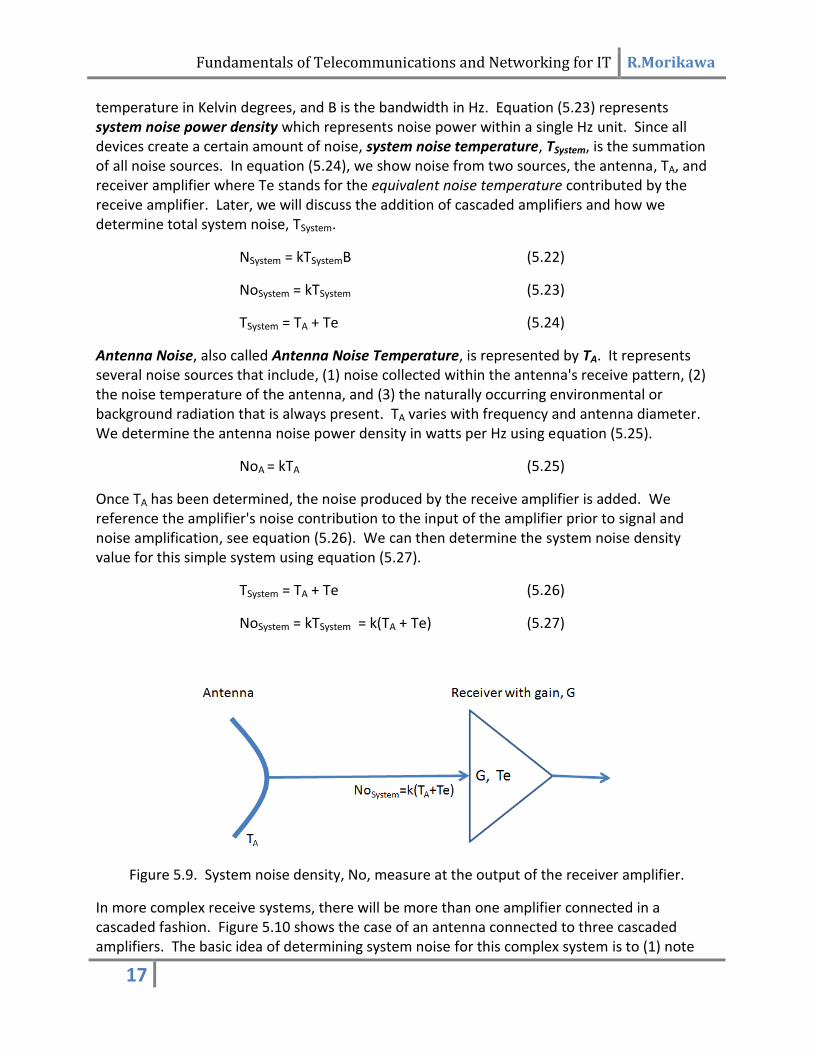
Once TA has been determined, the noise produced by the receive amplifier is added. We reference the amplifier's noise contribution to the input of the amplifier prior to signal and noise amplification, see equation (5.26). We can then determine the system noise density value for this simple system using equation (5.27).

TSystem = TA + Te (5.26)

NoSystem = kTSystem = k(TA + Te) (5.27)

Figure 5.9. System noise density, No, measure at the output of the receiver amplifier.

In more complex receive systems, there will be more than one amplifier connected in a cascaded fashion. Figure 5.10 shows the case of an antenna connected to three cascaded amplifiers. The basic idea of determining system noise for this complex system is to (1) note


18

that the amplifier's noise contribution is referenced to the input of the amplifier, (2) the amplifier's noise gain is seen at the output of the amplifier, and therefore figured into the input of the next amplifier in line, and (3) the amplifier gain is applied to both signal power as well as noise power, and therefore, if we wish to just determine total noise temperature, we must compensate for the noise gain products of each cascaded amplifier.

Figure 5.10. System noise temperature for the cascaded amplifier case.

Let's consider the three cascaded amplifiers in fig. 5.10(a). Each amplifier stage has an associated gain and output. The output of each stage is fed into the input of the following stage. We can treat this three stage system as a single amplifier shown in fig. 5.10(b), the gain, Gtotal equals the cumulative effect of all three amplifiers and Te is the equivalent noise temperature from all three stages. Therefore, if we wish to calculate the total noise contribution, Te, of all three cascaded amplifiers, we will need to solve equation (5.28).

Tout = Gtotal(Tin + Te) or Te = (Tout/Gtotal) - Tin (5.28)

Next, we turn back to fig. 5.16(a) and determine the output of each amplifier.

Tout1 = G1(Tin + Te1)

Tout2 = G2(Tout1 + Te2)

Tout3 = G3(Tout2 + Te3)

By combining the above equations, we simplify the noise temperature Tout3.

Tout3 = G3((G2(G1(Tin + Te1) + Te2)) + Te3)


19

= G3((G2(G1Tin +G1Te1) + Te2)) + Te3)

= G3((G1G2Tin + G1G2Te1) + G2Te2)) + Te3)

= G1G2G3Tin + G1G2G3Te1 + G2G3Te2 + G3Te3

Since Tout3 in fig. 5.10(a) equals Tout in fig. 5.10(b), we can substitute the above into eq. (5.28), where Gtotal = G1G2G3.

𝑇𝑒 = 𝑇𝑜𝑢𝑡

𝐺𝑡𝑜𝑡𝑎𝑙 − 𝑇𝑖𝑛 =

(G1G2G3Tin + G1G2G3Te 1 + G2G3Te 2 + G3Te 3)

𝐺1𝐺2𝐺3− 𝑇𝑖𝑛

= 𝑇𝑖𝑛 + 𝑇𝑒1 + 𝑇𝑒2

𝐺1+

𝑇𝑒3

𝐺1𝐺2 − 𝑇𝑖𝑛

𝑇𝑒 = 𝑇𝑒1 + 𝑇𝑒2

𝐺1+

𝑇𝑒3

𝐺2𝐺2

Finally, when we add antenna noise TA back into the above equation, we find our total system noise, equation (5.29).

𝑇𝑠𝑦𝑠𝑡𝑒𝑚 = 𝑇𝐴 + 𝑇𝑒1 + 𝑇𝑒2

𝐺1+

𝑇𝑒3

𝐺1𝐺2 (5.29)

Now that we know the system noise temperature, we can determine the system noise power, NSystem, noise power density, NoSystem, shown in equations (5.30) and (5.31) respectively.

NSystem = kTSystemB (5.30)

NoSystem = kTSystem (5.31)

We now have the information necessary to determine both the carrier over noise ratio (CNR) equation (5.32), and carrier over noise density, equation (5.33).

𝐶

𝑁 =

𝑃𝑅

𝑁𝑆𝑦𝑠𝑡𝑒𝑚 (5.32)

𝐶

𝑁𝑜 =

𝑃𝑅

𝑁𝑜 𝑆𝑦𝑠𝑡𝑒𝑚 (5.33)

Next we can include C/N and C/No into our link equations (5.11) and (5.12). Here, we are using the basic equations without adding cable losses or amplifier gains. This is done to simplify the following explanation. As we discussed earlier, gains and losses can easily be applied to the link calculation later.

We will derive the decibel and non-decibel equations for both C/N and C/No. For C/N, we take eq. (5.11) and substitute PR into eq. (5.32) to derive the non-decibel case.

𝐶

𝑁 =

𝑃𝑅

𝑁𝑆𝑦𝑠𝑡𝑒𝑚 =

𝐸𝐼𝑅𝑃∗ 𝐺𝑅

𝐹𝑆𝐿∗𝑘𝑇𝑆𝑦𝑠𝑡𝑒𝑚 𝐵 (5.34)


20

Converting eq. (5.34) into decibel form we get equation (5.35).

[C/N] = [EIRP] + [GR] - [FSL] - [k] - [TSystem] - [B] (5.35)

Similarly, for C/No, we substitute eq. (5.11) into eq. (5.33) and get equation (5.36) and (5.37), the later in decibel form.

𝐶

𝑁𝑜 =

𝑃𝑅

𝑁𝑜 𝑆𝑦𝑠𝑡𝑒𝑚 =

𝐸𝐼𝑅𝑃∗ 𝐺𝑅

𝐹𝑆𝐿∗𝑘𝑇𝑆𝑦𝑠𝑡𝑒𝑚 (5.36)

[C/No] = [EIRP] + [GR] - [FSL] - [k] - [TSystem] (5.37)

Note, that it is much easier to subtract other losses (e.g., cables, connectors, etc.) and add in gains (e.g., amplifiers) by using the decibel formats in eqs. (5.31) and (5.33), where these modifications are simple additions and subtractions to our overall calculation.

Example 5.7: Determine the [C/N] and [C/No] in decibels given the following information:

Frequency: f=12GHz, B (bandwidth) = 36MHz, d (distance between antennas) = 100 kilometers

Transmit-side: PT(Tx power)=100W, Parabolic Tx Ant. diameter DT =3 meters, T (ant. Eff.) = 55%

Receive-side: Parabolic Rx Ant. Dia. DR=1.5 meters, R = 45%, TSystem = 185K

Solution: = c/f = 3E8(m/s)/12E9Hz = 0.025 meters We want to solve for C/N and C/No using eqs. (5.35) and (5.37) in decibel form.

[C/N] = [EIRP] + [GR] - [FSL] - [k] - [TSystem] - [B] (5.35) [C/No] = [EIRP] + [GR] - [FSL] - [k] - [TSystem] (5.37)

Solve [EIRP] using eqs. (5.7) and (5.9),

GT = ((πD)/)2 = (0.55)(3π/0.025)2 = 78,167.27 [GT] = 10log10(78,167.27) = 48.93 dBi

[EIRP] = 10log10(100W/1W) + 48.93dBi = 20dBW + 48.93dBi = 68.93 dBW

Solve [FSL] using eq. (5.14),

[FSL](dB) = 20log10(4πd) - 20log10() = 20log10(4π100E3 m) - 20log10(0.025 m) = 121.98 dB - (-32.04 dB) = 154.02 dB Solve [GR] using eq. (5.7),

GR = (πD

)2 = (0.45)(1.5π/0.025)2 = 15,988.76

[GR] = 10log10(15,988.76) = 42.04 dBi

With the information determined above, we can determine C/N and C/No,


21

[C/N] = [EIRP] + [GR] - [FSL] - [k] - [TSystem] - [B]

= 68.93dBW + 42.04dBi - 154.02dB - 10log10(1.38E-23 J/K) - 10log10(185K) - 10log10(36E6Hz)

= 68.93 dBW + 42.04 dBi - 154.02 dB - (-228.60 dB) - 22.67 - 75.56 dB = 87.32 dB [C/No] = [EIRP] + [GR] - [FSL] - [k] - [TSystem]

= 68.93 dBW + 42.04 dBi - 154.02 dB - 10log10(1.38E-23 J/K) - 10log10(185K) = 68.93 dBW + 42.04 dBi - 154.02 dB - (-228.60 dB) - 22.67 = 162.88 dB 5.3.1.1 Noise Factor and Noise Figure

Besides using TSystem, there are two additional ways we can describe system noise. Noise factor measures the ratio of input noise power to output noise power of an amplifier. To ensure consistency when comparing noise factors, we always measure noise factor at a temperature of T=290K. The equation for noise factor, F, using noise power densities is shown in equation (5.38) where Nout is the output noise power density of the amplifier, Nin is the input noise density, G is amplifier gain, k is Boltzmann's constant (1.38E-23 J/K), and T=290K.

𝐹 = 𝑁𝑜𝑢𝑡

𝑁𝑖𝑛=

𝑁𝑜𝑢𝑡

𝐺𝑘𝑇 (5.38 )

We can also express noise factor in terms of the ratio of SNR input to SNR output as shown in equation (5.39).

𝐹 = 𝑆𝑁𝑅𝑖𝑛

𝑆𝑁𝑅𝑜𝑢𝑡 (5.39)

Noise figure, which is commonly used metric to determine the quality of an amplifier, is simply the decibel value of noise factor, see equation (5. ). [F] = 10log10F (5.40) 5.3.2 G/T, Receive System Figure-of-Merit

Receive antenna gain and total system noise contributed by receive system components play a critical role in determining the overall performance and efficiency of the communications link. As such we use the receive antenna gain over the total system noise as an important figure-of-merit, see equation (5.41).

GR/TSystem, or in decibels [GR] - [TSystem] (dBK-1) (5.41)

Since G/T is determined for a specific antenna and receive system, it is usually measured through testing once the system has been installed. Characterizing the antenna system involves taking G/T measurements and verifying these against calculated values. Because this


22

characterization is dependent upon the specific receive system setup, it needs to be re-characterized each time a major component of the system changes.

We can easily include G/T as part of our link equations by doing the following. We will work in decibels to simplify our task. We arrange eq. (5.35) as shown below, and simply replace [GR]-[TSystem] with [G/T] to come up with equation (5.42).

[C/N] = [EIRP] + [GR] - [TSystem] - [FSL] - [k] - [B]

[C/N] = [EIRP] + [G/T] - [FSL] - [k] - [B] (5.42)

Likewise, we can rearrange eq. (5.37),

[C/No] = [EIRP] + [GR] - [TSystem] - [FSL] - [k]

[C/No] = [EIRP] + [G/T] - [FSL] - [k] (5.43)

Once the receive antenna and system noise has been characterized in the form of G/T, it can be used to analyze link C/N or C/No, without the need of re-calculating system noise each time. It also provides a convenient metric for determining and comparing the quality of receive antenna systems.

Example 5.8: Given the previous example 5.7, determine the [G/T] of the receive antenna.

Solution: [G/T] = [GR] - [TSystem] = 42.04dBi - 22.67 dB = 19.37 dB/K

5.4 Data Rate Capacity

A primary goal for establishing a digital wireless link is to maximize resource efficiency, while achieving data rate maximization8. In order to maximize data capacity for a given situation, we need to consider the following.

Regulatory restraints on frequency and bandwidth assignments, as well as allowable transmit power. Since RF communications share a common medium with other RF signals, as well as from other EM noise sources, RFI becomes an issue. Therefore, regulatory agencies such as the Federal Communications Commission (FCC) at the national level, and International Telecommunications Union (ITU) at the international level, oversee frequency, frequency bandwidth, and power level allocations. Even devices operating at the unlicensed Industrial, Scientific and Medical (ISM) frequencies must adhere to specifications approved by these agencies.

Bit Error Rate (BER) tolerances for a given application and the use of error control methods as needed. A typical BER value for an unguided data link is 10-5. However, this BER value may be worse depending upon the noise environment. As such, error control

8 The data rate capacity of a link includes the information rate (i.e., the actual information being conveyed) plus

overhead data which includes framing and error control bits.


23

methods are used to reach an acceptable BER level. Any error control method used, whether error detection and retransmission, or error correction, adds additional bits to the link's overhead. This means that only a certain percentage of the data rate capacity transmitted will be true information. Therefore, if you were transmitting an uncompressed digitized voice grade signal of 64 kbps, you would need a higher capacity link that also included error control bits.

Noise products within the communication channel or link, including receive system noise temperature. This is closely related to BER tolerances. Depending upon the noise environment, an increase in noise causes a decrease in CNR, which translates into a lower achievable data rate capacity over the communications link.

Carrier power required at the receiver to enable signal detection. The amount of carrier power over noise (CNR), determines the amount of carrier power available to the receiver. Depending upon the specific receiver's sensitivity, is may or may not be enough power to enable signal detection. As an example, a receiver used in a satellite communications link would require a very sensitive receiver in order to detect a very weak signal from a distant satellite. Therefore, considering applicable regulatory constraints, you would perform a link analysis to determine the expected receive power, and select the appropriate receiver for the application.

Modulation scheme selected. M'ary modulation techniques increase the number of bits that a single symbol can represent. This means that for a given symbol rate, we can increase our data rate capacity; however this increase requires greater equipment complexity as well as better transmission conditions. So a noisy channel would be limited on on its use of complex modulation schemes.

Application for the communications link. Understanding the intended use of the communications link is a key driver in establishing the requirements that feed the ultimate design of the communications system. Tolerances in BER and the use of reliable error control schemes has a greater significance when sending medical imagery, than for sharing compressed .jpeg images. Establishing simple Push-To-Talk (PTT) links require a less complex system compared to a satellite phone service. By understanding the use of the communication link, we can design a system built around key objectives, whether they include costs, reliability, responsiveness, bulk capacity, etc.

We want a large enough data rate capacity to support our applications, but we also want as low an error rate as possible. Through link analysis, C/N and C/No can be determined. If we also know the desired BER and modulation method to be used, we can determine the data rate capacity that can be supported. In equation (5.44), C/N equals Eb/No (energy-bit per noise power density) multiplied by Rb (data rate) divided by BW (bandwidth). Eb/No stands for the energy per one bit, typically in units of Joules, over the noise power density in one Hz. Equations (5.44) and (5.46) represents C/N and C/No, respectively, as a function of Eb/No, data rate (Rb) and for eq. (5.44), bandwidth (BW). Equations (5.45) and (5.47) represent these equations in decibel form.


24

C/N = (Eb/No) x (Rb/BW) (5.44)

[C/N] = [Eb/No] + [Rb] - [BW] (5.45)

C/No = (Eb/No) x Rb (5.46)

[C/No] = [Eb/No] + [Rb] (5.47)

Let's consider eq. (5.45). If we know [C/N], [Eb/No], and [BW], then we can solve for [Rb],

[Rb] = [C/N] - [Eb/No] +[BW] (5.48)

The value for Eb/No is typically derived from a graph such as the one in figure 5.11. The curve represents NRZ line coding, as well as BPSK and QPSK modulation methods, and associates BER with required Eb/No levels in decibels. Note that typical graphs such as this will display several curves that represent numerous M'ary and line coding methods. In the example in fig. 5.11, if we wish to achieve a BER = 10-5 using BPSK modulation, then the required [Eb/No] = 9.7dB. If we also know the bandwidth of our signal, then we can determine the data rate using eq. (5.48).

Figure 5.11. BER Versus Eb/No diagram taken from Roddy, D. (2006). Satellite Communications 4th

Ed. New York: McGraw-Hill.


25

Example 5.9: Using eq (5.48) and the graph in fig. 5.11, determine the data rate capacity given the following. [C/N]= 40 dB, BW = 6 MHz, desired BER=10-5.

Solution: With a desired BER of 10-5, we determine a required [Eb/No] value of 9.7dB. Using eq. (5.48),

[Rb] = [C/N] - [Eb/No] +[BW] = 40dB - 9.7dB + 10log10(6E6)

= 40dB - 9.7dB + 67.78dB = 98.08 dB

We convert [Rb] from decibels to data rate,

Rb = 10(98.08/10) = 6.43 Gbps

5.5 Multipath and MIMO

Multipath propagation occurs in all unguided communications links. It is based upon the fact that electromagnetic waves will travel at the speed-of-light. A transmitted RF signal will spread as it propagates in free space, which means that some paths of the signal may encounter signal impairments such as reflection (see fig. 4.17), while others may be direct line-of-sight (LOS) to the receive antenna. Since all signal paths propagate at the same velocity, path lengths will vary, thus causing copies of the same signal to reach the receiver at slightly different times resulting in signal distortion. Figure 5.12 shows the transmitted signal taking several different paths. L1 is the shortest distance, direct LOS path and therefore this signal will reach the receive antenna first. The other signals, L2 through L4, take different paths and are therefore subjected to different impairments such as reflection by one or more objects. This causes copies of the same signal to reach the receiver at slightly different times. The out-of-phase copies destructively combine together with one another, creating distortion of the original signal at the receiver which is termed multipath fading.


26

Figure 5.12. Multipath Propagation. A signal takes several different paths from the Tx antenna to the Rx antenna. Since all waves propagate at the same speed-of-light, the shorter distance,

L1 reaches the Rx antenna first, followed by L2, L3 and L4. Multiple copies of the signal reaching the receiver at slightly different are destructively combined causing signal distortion.

One way to reduce the adverse effects of multipath is to buffer incoming signal copies during a specified sampling period, and then send these copies to a digital signal processor (DSP) that adjusts the phase angle of each copy received. Once the signal copies are adjusted to the same phase angle, they can be constructively combined to create an amplified receive signal.

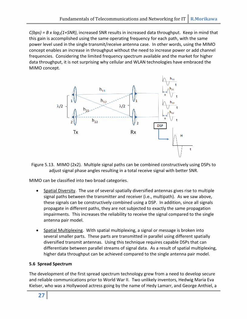
While multipath propagation is typically undesirable between single transmit and receive antennas, it can be used to significantly improve data capacity when combined with multiple spatially diversified transmit and receive antennas, and DSPs. This concept is termed Multiple Input, Multiple Output (MIMO) and it is a method used today in WLAN (wireless LAN, 802.11n), and 4G cellular standards such as LTE (Long Term Evolution) and WiMAX (802.11e). Figure 5.13 represents a 2x2 MIMO system of four antennas9, two transmit and two receive. The two antennas located at either transmission ends are separated by approximately one-half wavelength or less. Tx antenna 1 has a direct LOS path to Rx antenna 1 (h11), and an indirect path to Rx antenna 2 (h12). Likewise, Tx antenna 2 has a direct LOS path to Rx antenna 2 (h22), and an indirect path to Rx antenna 1 (h21). The indirect paths, h12 and h21, have longer distances to travel thus these signal will arrive later in time than the direct LOS signals h11 and h22. In addition these indirect paths may be reflected by objects within the environment, causing even greater signal delay. By using DSPs to adjust the timing (i.e., phase) of the direct and indirect signals from both receive antennas and then constructively combining them, we will realize a gain in the total signal power received. Per Shannon-Hartley's Capacity Theorem,

9 Any number of transmit or receive antennas can be used with the MIMO concept.


27

C(bps) = B x log2(1+SNR), increased SNR results in increased data throughput. Keep in mind that this gain is accomplished using the same operating frequency for each path, with the same power level used in the single transmit/receive antenna case. In other words, using the MIMO concept enables an increase in throughput without the need to increase power or add channel frequencies. Considering the limited frequency spectrum available and the market for higher data throughput, it is not surprising why cellular and WLAN technologies have embraced the MIMO concept.

Figure 5.13. MIMO (2x2). Multiple signal paths can be combined constructively using DSPs to adjust signal phase angles resulting in a total receive signal with better SNR.

MIMO can be classified into two broad categories.

Spatial Diversity. The use of several spatially diversified antennas gives rise to multiple signal paths between the transmitter and receiver (i.e., multipath). As we saw above, these signals can be constructively combined using a DSP. In addition, since all signals propagate in different paths, they are not subjected to exactly the same propagation impairments. This increases the reliability to receive the signal compared to the single antenna pair model.

Spatial Multiplexing. With spatial multiplexing, a signal or message is broken into several smaller parts. These parts are transmitted in parallel using different spatially diversified transmit antennas. Using this technique requires capable DSPs that can differentiate between parallel streams of signal data. As a result of spatial multiplexing, higher data throughput can be achieved compared to the single antenna pair model.

5.6 Spread Spectrum

The development of the first spread spectrum technology grew from a need to develop secure and reliable communications prior to World War II. Two unlikely inventors, Hedwig Maria Eva Kielser, who was a Hollywood actress going by the name of Hedy Lamarr, and George Anthiel, a


28

musician, worked together on an invention that eventually led to today's frequency hopping spread spectrum (FHSS) concept. The device described in their 1942 patent involved a mechanical system that could rapidly change transmission frequencies during a communications session. Only the transmitter and intended receiver would know the correct sequence of frequency changes, therefore making eavesdropping nearly impossible. By rapidly changing the frequency during a communications session, the signal appeared to be spread over a large frequency bandwidth, making narrowband jamming extremely difficult. Although patented, the U.S. military did not take the patent seriously during the war. It was not until the 1950s, after electronic technologies had made numerous advances, that Lamarr's patent resurfaced to begin the era of development on spread spectrum communications.

The basic idea of spread spectrum, is to spread narrowband signals into a much wider band, thus increasing spectral efficiency and improving communications security. Multiple communication sessions exist within the same frequency bandwidth, separated by unique Pseudorandom Noise (PN) codes that are only shared between communicating devices. The PN codes describes two aspects: (1) pseudorandom describing that the code is not truly random, but deterministic, and (2), that spreading the signal in the frequency domain without adding additional signal power causes the signal to appear as wideband noise vice a signal. There are two main spread spectrum techniques used today,

Direct Sequence Spread Spectrum (DSSS). With DSSS, an information data rate is combined with a PN code to produce a higher data rate which is termed the chipping rate. The higher chip rate causes the original non-spread signal to expand in bandwidth. This process will be discussed further in section 5.6.1.

Frequency Hopping Spread Spectrum (FHSS). Similar to Lemarr's original 1942 patent, the concept behind FHSS is to rapidly change transmission frequencies during a communications session. Unlike Lamarr's version, FHSS is implemented on high speed firmware chips used on both the transmit and receive systems. A shared pseudorandom hop sequence enables both transmitter and receiver to be on the same frequency to send and collect data. An example of FHSS in use today is IEEE 802.15 where Bluetooth devices operate at 1600 frequency hops per second over a 79 MHz bandwidth.

5.6.1 A Closer Look at DSSS

Direct Sequence Spread Spectrum (DSSS) techniques have been used in 802.11 Wireless Local Area Networks (WLAN). In addition, Code Division Multiple Access (CDMA) is a form of DSSS used in 2G and 3G cellular phone networks. DSSS techniques have several advantages when compared to narrow band channels. This first is its survivability in an environment where interfering noise, to include intentional signal jamming10, is present. In the upper graph of figure 5.14, we see how a narrow band interfering noise source will only disrupt part of a spread signal. Because most of the signal energy is left undisturbed, use of DSSS results in a more reliable communications link when operating in a noisy environment.

10

Most signal jammers are narrow band since it take enormous amounts of power to jam a wideband signal.


29

The second advantage when using DSSS is its spectral efficiency. In the lower graph of fig. 5.14, we have superimposed several narrow band FDM channels over spread signals for comparison. The FDM channels must be separated by guard channels in order to avoid interference between channels (i.e., intermodulation, IM, noise). Unfortunately, no information can be transmitted within these guard bands, therefore it represents unused frequency spectrum. When we consider the limited availability of frequency spectrum combined with today's desire for higher data throughput, the use of guard channels that carry no data becomes costly in terms of spectral efficiency. DSSS eliminates the need for guard channels since users occupy the entire frequency bandwidth and are separated by unique PN codes. By eliminating the need for guard channels, an increase in spectral efficiency is realized, which leads to increased data throughput.

A third benefit is greater security from data interception that each pair of users enjoy. Since unique PN codes are required for each communicating pair, it is much more difficult to intercept and process user information without knowledge of the PN code being used. This enhances privacy to a much greater extent than FDM, where one only needs to know the frequency channel of interest to collect communication data.

In order to successfully implement DSSS, a unique set of orthogonal PN codes must be created. These codes are used by each communicating pair to increase the information data throughput to a much higher chipping rate (see Figure 5.15). According to Shannon-Hartley theorem, increasing throughput results in an increase of the frequency bandwidth occupied by the signal. Since no power is added during the spreading process, the resulting spread signal appear flattened with a lower amplitude than the narrowband signal. This is due to the fact that the pre-spread narrowband signal has the same power density as the post-spread signal as shown in figure 5.15.

Shannon-Hartley Theorem: C(bps) = B x log2(1+SNR)


30

Figure 5.14. The upper plot shows a spread signal in the frequency domain with an interfering noise source identified. The noise source only effects a small portion of the spread signal,

therefore most of the signal is not impacted by the noise and the signal can get through to the receiver. The lower plot shows a comparison between multiple narrowband channels that

require separation by guard channels, compared to the spread spectrum signal which eliminate the need for guard channels and therefore increases spectral efficiency.

Figure 5.15. Direct Sequence Spread Spectrum (DSSS). A narrowband signal is spread over a wider bandwidth after being combined with the PN code. The area under the each curve,

narrowband and spread signal, represents power density and are equal. As a result, the spread signal has a lower amplitude and appears more flattened.

In order to explain how DSSS works, we will now go over a simple example. The first requirement is to identify a set of orthogonal PN codes for use. An N bit code word will, at the most, have N number of orthogonal PN codes associated with it. As an example, let's say we decide to use a four bit PN code which gives us 24=16 permutations. However, only 4 of the 16


31

permutations will give us orthogonal PN codes. In order to be an orthogonal PN code, it must have zero correlation with any other PN code word. This test for orthogonality is accomplished by determining the dot product between any two PN code words in the set. Instead of using logical 1's and 0's as values in our PN code we will instead use voltage levels, either 1v or -1v. Therefore our four orthogonal codes are represented by:

PN1 = (1v, 1v, 1v, 1v) PN2 = (1v, 1v, -1v, -1v) PN3 = (1v, -1v, 1v, -1v) PN4 = (1v, -1v, -1v, 1v)

An two PN codes are orthogonal provided their dot product equals zero. Therefore, we can test each combinations of PN codes in our set of four (note: the below dot products assume units of voltage). The resulting products confirm that the four PN codes represent an orthogonal code set.

PN1 PN2 = (1*1) + (1*1) + (1*-1) + (1*-1) = 1 + 1 +(-1) + (-1) = 0

PN2 PN3 = (1*1) + (1*-1) + (-1*1) + (-1*-1) = 1 +(-1) +(-1) + 1 = 0

PN3 PN4 = (1*1) + (-1*-1) + (1*-1) + (-1*1) = 1 + 1 +(-1) + (-1) = 0

PN4 PN1 = (1*1) + (-1*1) + (-1*1) + (1*1) = 1 + (-1) +(-1) + 1 = 0

With the four PN codes identified, we can now support four simultaneous user connections, with each transmitter and receiver pair sharing a single PN code. Table 5.1 shows a list of assigned PN codes for users 1 through 4, and the data each user wishes to send to the receiver.

Table 5.1. Direct Sequence Spread Spectrum Example - user assignment of PN codes and data to be transmitted

User Tx/Rx Pair

Assigned PN Code Data to be sent

User 1 PN1 = 1, 1, 1, 1 D1 = 1, 1, 1

User 2 PN2 = 1,1,-1,-1 D2 = 1, -1, -1

User 3 PN3 = 1,-1,1,-1 D3 = -1, -1, 1

User 4 PN4 = 1,-1,-1,1 D4 = -1, 1, -1

The next step is to combine the user data with the PN code using an XOR logic gate in order to expand the data rate to the spread chipping rate. The XOR logic table 5.2 is shown below which uses 1V and -1v vice logical 0's and 1's.


32

Table 5.2. XOR Logic table using voltage levels.

Combining each user's PN code with the user's data using the XOR logic results in the below,

User 1: PN1 ⊕ D1 = 1v,1v,1v,1v 1v,1v,1v,1v 1v,1v,1v,1v

User 2: PN2 ⊕ D2 = 1v,1v,-1v,-1v -1v,-1v,1v,1v -1v,-1v,1v,1v

User 3: PN3 ⊕ D3 = -1v,1v,-1v,1v -1v,1v,-1v,1v 1v,-1v,1v,-1v

User 4: PN4 ⊕ D4 = -1v,1v,1v,-1v 1v,-1v,-1v,1v -1v,1v,1v,-1v

The sum of the four user voltages above represents the aggregate voltage signal that appears on the shared bandwidth.

Aggregate Total = (PN1 ⊕ D1) + (PN2 ⊕ D2) + (PN3 ⊕ D3) + (PN4 ⊕ D4)

User 1: PN1 ⊕ D1 = 1v,1v, 1v, 1v 1v, 1v, 1v,1v 1v, 1v,1v, 1v User 2: PN2 ⊕ D2 = 1v,1v,-1v, -1v -1v,-1v, 1v,1v -1v,-1v,1v, 1v User 3: PN3 ⊕ D3 = -1v,1v,-1v, 1v -1v, 1v,-1v,1v 1v,-1v,1v,-1v User 4: PN4 ⊕ D4 = -1v,1v, 1v, -1v 1v,-1v,-1v,1v -1v, 1v,1v,-1v Aggregate Total = 0, 4v, 0, 0 0, 0, 0, 4v 0, 0, 4v, 0

The aggregate total voltage signal is seen by all users, however unique PN codes separate the data for each user. As an example, if User 3 applies PN3 code to the aggregate signal, then the data for User 3 will be revealed. User 3 multiplies the aggregate signal with PN3: PN3: 1v,-1v,1v,-1v 1v,-1v,1v,-1v 1v,-1v,1v,-1v Aggregate Total: 0, 4v, 0, 0 0, 0, 0, 4v 0, 0, 4v, 0

0, -4v, 0, 0 0, 0, 0, -4v 0, 0, 4v, 0

Divide by 4 (4 PN codes) and the data becomes -1v, -1v, 1v, which is User 3 D3 per tab. 5.1. It is left as an exercise for students to verify that User 1, 2 and 4 data can be extracted from the aggregate signal.


33

5.7 Orthogonal Frequency Division Multiplexing (OFDM)

Orthogonal Frequency Division Multiplexing (OFDM) is a multicarrier modulation concept in which user data is transmitted in parallel over several subcarriers. Figure 5.16(a) represents typical FDM channels that are separated by guard bands. In comparison, fig. 5.16(b) represents OFDM where the subcarriers overlap one another, thus increasing spectral efficiency and throughput. The spacing of the subcarriers is critical in order to enable overlapping; a situation that would cause intermodulation noise in FDM applications. The subcarriers are orthogonal to one another, meaning that the subcarrier spacing equals one over the period of the symbol, or one over symbol-time, 1/Tsymbol. Doing this creates signal nulls from adjacent subcarriers. Essentially, this means that when we collect the center frequency of a subcarrier, the adjacent subcarriers present a null or zero signal at our center frequency. This leave only the center frequency which is what we desire to collect.

Figure 5.16. Orthogonal Frequency Division Multiplexing (OFDM). (a) represents typical FDM channels which are separated by a guard band. (b) represents OFDM subcarriers which can

overlap, thus increasing spectra efficiency.

Even though each subcarriers has a smaller bandwidth, transmitting data over several subcarriers in parallel increases data throughput when compared to DSSS and FDM. In addition, while it is not a spread spectrum technique, it has the benefit of transmitting a signal over a wider bandwidth using several subcarriers. As such, OFDM has greater resiliency from noise and fading similar to spread spectrum. OFDM has been implemented in many of today's communications standards such as 802.11n, 802.11ac, DSL (Digital Subscriber Line), WiMAX 802.16e, and LTE-Advanced.


34

A popular version of OFDM is Coded Orthogonal Frequency Multiplexing (COFDM) which incorporates an error correction capability.

Orthogonal Frequency Division Multiple Access (OFDMA) is an access scheme used by service providers that assigns several subcarriers to a user. Other examples of assigning resources to users are Frequency Division Multiple Access (FDMA), Time Division Multiple Access (TDMA), and Code Division Multiple Access (CDMA).


35

Key Terms - Ch5

Antenna Efficiency () Antenna gain Antenna noise temperature Antenna polarization Antenna Reciprocity BER Carrier-to-Noise Ratio (CNR) Circular Polarization CoPolar Cross Polar Directionality Direct Sequence Spread Spectrum (DSSS) Eb/No Effective aperture (Ae) EIRP EM wave polarization Frequency Hopping Spread Spectrum (FHSS) Frequency Reuse Friis Free Space Loss G/T Horizontal Polarization Ideal isotropic antenna Impedance Left Hand Circular Polarization (LHCP)

Linear Polarization Link Analysis Multiple Input, Multiple Output (MIMO) Multipath Noise Factor Noise Figure Non-resonant Orthogonal Orthogonal Frequency Division Multiplexing (OFDM) Parabolic reflector Power density Pseudorandom Noise Code Reactive components Receive sensitivity Resistive components Resultant Wave Resonance Right Hand Circular Polarization (RHCP) Spatial Diversity Spatial Multiplexing System Noise Temperature Vertical Polarization


36

Chapter 5 Problems: 1. The "Reciprocity Theorem for Antennas" states that the transmitting and receiving characteristics are the same for identical antennas operating at the same wavelength. a. True b. False Answer: a

2. An /2 dipole operating at a frequency of 900MHz will have a length of _______ meters.

Answer: = c/2f = (3E8 m/s)/(2*900E6 Hz) = 0.167 meters 3. An "ideal isotropic antenna" is a hypothetical antenna that has an efficiency of 100%. a. True b. False Asnwer: a 4. When describing the antenna gain of directional antenna in decibels, we typically use an isotropic antenna as the reference (i.e., dBi). a. True b. False Answer: a 5. Antenna "gain" refers to the power density increase of a directional antenna in a given direction, over that of the ideal isotropic antenna. Gain is typically given in "dBi" which compares the ratio between a directional antenna and an ideal isotropic antenna. a. True b. False Answer: a 6. In an E-M wave, the E-field defines the polarization of both the antenna and E-M wave. a. True b. False Answer: a 7. Select the correct statement regarding antenna and E-M wave polarization. a. A vertically polarized antenna can communicate with a horizontally polarized antenna b. A vertically polarized antenna can only communicate with another vertically polarized antenna c. An E-M wave emitted from a vertically polarized antenna will be horizontally polarized d. All of the statements are correct Answer: b 8. A linearly polarized antenna (i.e., vertical or horizontal) will typically have components in both the horizontal and vertical poles (i.e., co-polar and cross-polar components). a. True b. False Answer: a


37

9. Depolarization of the E-M wave causes polarization misalignment, which results in a weaker resultant wave and less power transfer from E-M wave to antenna. a. True b. False Answer: a 10. A RHCP antenna is orthogonal to a LHCP antenna. a. True b. False Answer: a 11. An antenna can transmit two different signals on the same frequency by ensuring that both signals are orthogonally polarized (i.e., vertical and horizontal, or RHCP and LHCP). This is a method used for frequency re-use. a. True b. False Answer: a 12. Select the correct statement regarding cross polarization. a. Cross polarization between two linear antennas can cause a 30dB loss in signal b. Cross polarization between two linear antennas can increase signal strength by 30dB c. Cross polarization is not a problem for earth terminals communicating with satellite in space d. both b and c are correct Answer: a 13. What can cause cross polarization? a. Ionosphere, radiation, meteors b. Ionosphere, ice crystals, rain c. Ionosphere, temperature, clouds d. Ionosphere, cosmic rays, x-rays, Answer: b 14. Select the correct statement(s) regarding an antenna's "Effective Aperture". a. The effective aperture describes the physical dimensions of the antenna b. The effective aperture describes that part of the physical aperture that is actively involved in

transmission and reception of power density c. The effective aperture is a theoretical antenna, similar to the ideal isotropic antenna but for

directional antennas, that is not realistically achievable d. Both a and c are correct Answer: b 15. Select the correct statement(s) regarding the gain of a parabolic antenna. a. Antenna gain increases as the diameter of the antenna increases b. Antenna gain increases as the transmit frequency increases c. Antenna gain increases as antenna efficiency increases d. All of the above are correct Answer: d


38

16. EIRP (effective isotropic radiated power) decrease as antenna gain increases. a. True b. False Answer: b 17. What is the effective antenna aperture, Ae, of a parabolic 3 meter antenna where efficiency, η is 75%? (Ae= ηA and A= πD2/4) a. 5.3 m2 b. 53 m2 c. 0.53 m2 d. 7.07 m2 Answer: a 18. What is the gain, G,in decibels ([G] = G(dB)), of a 9 meter parabolic antenna aperture operating at a frequency of 12GHz, with an antenna efficiency, η is 60%? a. [G] = 68.85 dBi b. [G] = 48.85 dBi c. [G] = 58.85 dBi d. [G] = 38.85 dBi Answer: c 19. What is the thermal noise power given T=290 Kelvin, and BW=40,000Hz in watts and dBWs? a. 1.6E-23, -1.28E2 b. 2E-16, -1.28E2 c. 1.6E-16 W, -1.58E2 dBW d. 2E-23, 1.58E2 dBW Answer: c 20. Determine thermal noise density (No=kT) in watts and dBs, at a receiver operating at a temperature of 295 degrees Kelvin. a. 4.1E-21, -203dBW b. 4.1E21, 203dBW c. 1.42E-16, -203dBW d. -1.42E-21, 203dBW Answer: a 21. While a receiver provides gain to the signal and noise received at its input, it also contributes its own noise. a. True b. False Answer: a 22. Select the correct statement(s) regarding SNR and CNR. a. SNR is measured at the input to the receiver b. CNR is measured at the input of the receiver c. CNR equals SNR plus receiver processing gain d. There is no difference between CNR and SNR Answer: b


39

23. Determine the C/N in dB given the following: Pr=-50dBm, T=290 Kelvin degrees, B (bandwidth) = 36MHz. a. [N]=-158.41dBW, [C/N]=138.41dB b. [N]=-158.41dBW, [C/N]=78.41dB c. [N]=-128.41dBW, [C/N]=148.41dB d. [N]=-128.41dBW, [C/N]=48.41dB Answer: d 24. Determine the C/No required in decibels to support a 256 kbps link using BPSK modulation and a desired BER of 1E-4, using an Eb/No = 8.5dB. a. [C/No] = 62.6 dB b. [C/No] = 53.6 dB c. [C/No] = 256E3 dB d. Insufficient information to complete calculation Answer: a 25. The C/No at your receiver is 60dB and you are attempting to push a data rate of 512kbps. (a) What is your Eb/No, and BER from Fig 10.17 (in your text). (2) What will be the performance of your link? a. [Eb/No]=117dB, your BER would be very high and the performance of your link will be excellent b. [Eb/No]=8.5dB, at a BER between 1E-1 and 1E-2, your link would be inadequate c. [Eb/No]=3dB, at a BER between 1E-1 and 1E-2, your link would be inadequate d. Insufficient information to complete calculation Answer: c 26. Determine the power measured, Pr, at the receiver in decibels given the following: Data rate = 40kbps [Eb/No] for a desired BER of 1E-6 is: 10.4dB Noise Temperature in Kelvin is 290 degrees Receive frequency bandwidth is 80kHz (N = kTB, [C/N](dBs) = [Eb/No]+[Rb]–[BW], C = Pr) a. [N]=-185dBW, [C/N] = 17.4dB, C=Pr=-177dBW b. [N]=-175dBW, [C/N] = 4dB, C=Pr=+147dBW c. [N]=-155dBW, [C/N] = 7.4dB, C=Pr=-147dBW d. Insufficient information to complete calculation Answer: c 27. Determine [FSL] in decibels given a distance between Tx and Rx of 10,000km, and an operating frequency of 9GHz. a. [FSL] = 191.53 dB b. [FSL] = 291.53 dB c. [FSL] = 91.53 dB d. [FSL] = 1915.3 dB Answer: a


40

28. Given the following information, what data rate (Rb) can be supported? C/No=50dBW, Eb/No=8.4dB a. 14,454 bps b. 41.6 bps c. 144kbps d. Insufficient information available to determine maximum data rate Answer: a 29. Your earth station has a G/T of 20 dB/K. Given the following, what is the C/No at the receive earth station? Satellite EIRP = 35 dBW Losses = FSL + 2dB additional losses Distance between satellite and earth station = 35,000 km frequency = 9GHz a. [C/No] = 179.2 dB b. [C/No] = 184.6 dB c. [C/No] = 79.2 dB d. [C/No] = 88.2 dB Answer: c 30. Select the correct statement(s) regarding multipath. a. Multipath results in several copies of a signal being received at slightly different times by the receiver,

thus causing signal distortion b. Multipath is not a problem in urban environments where large buildings easily block multiple copies

of a single signal c. Multipath is only a problem when transmitting analog signals (e.g., AM and FM radio) d. All of the above are correct Answer: a

31. CDMA (Code Division Multiple Access) is a form of DSSS (Direct Sequence Spread Spectrum) where users share the same frequency bandwidth, separated by unique PN (Pseudorandom Number) codes. a. True b. False Answer: b

32. Select the correct statement regarding signal propagation: a. The higher the frequency, the greater the attenuation b. The higher the frequency, the greater the need for Line-of-Site (LOS) c. The higher the frequency, the greater the capacity to carry information d. All of the above are correct Answer: d

33. With Orthogonal Frequency Division Multiplexing (OFDM), a user is assigned a set of "sub-carriers" for parallel data transmission and reception. Using OFDM allows the service provider to more efficiently use valuable frequency allocations when compared with FDM. a. True b. False Answer: a

chapter 5. rf wireless communications 5.4 data rate ...mason.gmu.edu/~rmorika2/chapter 5 riki v4...

Documents