chapter 5 assessing result and analyzing the...

CHAPTER 5

ASSESSING RESULT AND ANALYZING THE CHOSEN ROUTE

5.1 Introduction

This chapter will show the results of implementing the methodology discussed in

chapter 4 with the input data in chapter 3. The process in the methodology, as explained

in chapter 4, is repeated several times in different settings. In this chapter, all settings,

output and the output assessment results will be shown. However, due to the similarity

of the output results and to avoid repetition, there will be just one example output

assessment explained step-by-step. After describing the assessment process, this chapter

will then show the variations of setting and results. Next, the results will be compared

and the best result will be determined. Finally, the best route will then be detailed and

analyzed for enhancing the optimum output.

5.2 Route Assessment

This chapter will use the example data from chapter 4 in the assessment process of the

output. This section will start with the setting of the route destination in the following

figure.

145

Figure 5.1 The routes setting (example)

The above figure is taken from a section in chapter 4 pertaining to inspecting the

number of routes that are needed to cover all orders. In this chapter, the purpose of the

setting is to make a destination of 4 depots in the different directions (north, south, west,

and east) by setting orders, depots, and route classes. This example will generate an

output like the one shown in figure 5.2 below.

146

Figure 5.2 The output (example)

The above output will then be processed and combined with the model in figure

4.34 from section 4.9.1. The four route directions will then be buffered to get each

surrounding area, followed by a calculation to determine the needy in that area. Figure

5.3 shows the covered area in the surrounded area of all route directions. The area is

shown in graduate color from light grey to black. The darker the color is, the greater the

number of needy student who live there. Areas with no color (white) indicate no route

coverage. Those areas have distances which exceed 300 meters in any direction of the

street which participate in the route.

147

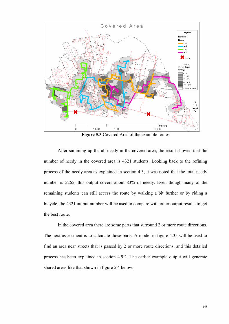
Figure 5.3 Covered Area of the example routes

After summing up the all needy in the covered area, the result showed that the

number of needy in the covered area is 4321 students. Looking back to the refining

process of the needy area as explained in section 4.3, it was noted that the total needy

number is 5265; this output covers about 83% of needy. Even though many of the

remaining students can still access the route by walking a bit further or by riding a

bicycle, the 4321 output number will be used to compare with other output results to get

the best route.

In the covered area there are some parts that surround 2 or more route directions.

The next assessment is to calculate those parts. A model in figure 4.35 will be used to

find an area near streets that is passed by 2 or more route directions, and this detailed

process has been explained in section 4.9.2. The earlier example output will generate

shared areas like that shown in figure 5.4 below.

148

Figure 5.4. Shared areas of example output which have access to 2 or more route directions

Figure 5.4 above has surrounded areas with gradation colors from light green to

dark green. Again, the darker the color appears is an indication of the greatest numbers

of needy. There are few shared areas between west and north route directions in the

west part and a medium shared area in the east between south and east route directions.

There is a major shared area in the center part which is due to an accumulation of

shared areas between east and south, north and south, north and east, and south and

north route directions. With the similar calculation used in summing up the covered

needy, all the shared areas cover 1840 needy. In summary, this means there is 34% of

needy that can choose more than 1 route direction.

The next process is to find shared areas that have access to 3 or more route

directions. The process is shown in figure 4.35 and explained in section 4.9.3. If the

previous process is to generate a union or common area from all intersection of 2

combined route directions, then this process will make a union from all intersections of

3 route direction combinations. The generated area is a subset of the previous one.

149

Figure 5.5 shows the result of this process in gradations of red. The total number of

students in this area is 549.

Figure 5.5. Shared areas of example output which have access to 3 or more route directions.

Figure 5.6. Shared areas of example output which have access to 4 route directions

150

Using a similar process, by increasing the number of route directions in the

combination, the shared area with 4 route directions can be generated. The process is

modeled in figure 4.28. This process will generate a result similar to figure 5.6. The

area is small, basically a circle area around the starting depot, and there are 200 needy

covered. Because of its rare appearance, except for at the starting depot location, this

last shared area will not apply in the others’ variation of setting.

The next point to be assessed is the load balance. Each route direction will be

separated, then processed using a similar step like that used in the finding the covered

area. This time, each route direction will be processed independently. The total covered

needy per direction will then be compared with the total capacity of schools in that

direction. The process is modeled in figure 4.38 and 4.39. The result of this process is

outlined in figure 5.7 below.

Figure 5.7. The 4 route directions including their covered areas and schools

151

Figure 5.7 shows the 4 route directions as well as their covered areas and

schools. This figure shows the routes in different colors: the west route is colored in

green, the east route in magenta, the north in cyan, and the south in dark yellow. The

schools, symbolized using dots of the same route color, appear similar in numbers

across the 4 routes. Moreover, there are routes that cover schools whose location is not

its directed area. This is because the VRP engine does not travel across specific

separated schools. In other words, it was free to deliver passengers to any school while

traveling within the minimum time consumed from the start depot to each destination.

This non-assigned school may take the route which will lead to a bad balance which

will have a negative impact. Table 5.1 shows the school in each separated area and the

total capacities. These totals are then compared with the number of covered needy.

152

Table 5.1 Schools separated by routes and capacity

NameRoute Name

Minutes bus arrived

Needy capacity

SMP Tri Tunggal VII east 63 97

SMP Romly Tamim east 76 118

SMP PGRI XI east 79 150

SMP Terbuka 18 east 82 152

SMP Negeri 18 east 84 154 Capacity east 671

SMP Gatra north 5 91

SMP UNESA 1 SURABAYA north 10 125

SMP Kawung 1 Surabaya north 12 51

SMP Bina Bangsa north 16 134

SMP Terbuka 5 north 18 149

SMP Negeri 5 north 20 68

SMP Katolik Angelus Custos north 24 154

SMP GATOTAN 1 SURABAYA north 26 150

SMP Negeri 2 north 29 154

SMP Ta'miriyah north 31 154

SMP Muhammadiyah 1 north 37 119

SMP Wachid Hasyim I north 43 99

SMP MUHAMMADIYAH 16 north 50 30

SMP PGRI VI SBY north 53 110

MTs Nurul Salam north 56 13

SMP Cahaya north 59 134

SMP Negeri 27 north 61 147 capacity north 1882

SMP Taruna Jaya I south 23 143

SMP Muhammadiyah 15 south 31 132

SMPK. Pecinta Damai south 33 148

SMP YP 17 SURABAYA south 36 93

SMP ISLAM LIL WATHON south 44 41

SMP ISLAM AL AMAL south 47 39

SMP ALKHAIRIYAH south 51 100

SMP AL GHOZALI south 54 125

SMP AL IRSYAD SURABAYA south 56 115

SMP Ganesya I Surabaya south 64 75

SMP Negeri 8 south 66 136

SMP Triyasa south 70 148

SMP YPPI 1 south 73 147

SMP Negeri 41 south 76 74 capacity south 1516

SMP Mujahidin west 7 109

SMP PGRI 36 west 10 121

SMP Barunawati west 14 127

SMP Negeri 7 west 18 149

SMP K St. Mikael west 20 125

SMP Al-Ikhlash west 22 149

SMP Hang Tuah-4 Surabaya west 25 130

SMP PGRI 5 Surabaya west 29 146

SMP Kemala Bayangkari 6 west 33 112

SMP Islam west 38 72

SMP Muhamadiyah XI west 44 95

SMP Bina Karya west 52 76 capacity west 1411

153

After summing up the needy in each route destination area, it found that in terms

of needs coverage, the west route covers 1130, the east route covers 2163, the north

route covers 1377, and the south route covers 2239. The sum of these covered areas is

more than the covered area discussed in last section the previous paragraph. As

explained earlier, it is due to the fact there are shared areas. Meanwhile, in the west

area, there are 12 schools with a total capacity of 1411, in the east 5 schools with 671

capacity, a north area consisting of 17 schools with 1882 capacity, and a south area with

a total capacity of 1516. The comparison is as follows: there are 1130 needy for 1411

school seats in the west, 2136 needy for 671 school seats in the east, 1337 needy for

1882 school seats in the north, and finally 2239 needy for 1516 school seats in the

south. The west and north areas have a less number of needy, while the east and south

area have an excess one. We can conclude from these finding that this proposed route

is not as good in terms of the route balance.

Another important aspect which must be assessed is the time consumed. The

time consumed is a total of each direction route’s traveling time. This traveling time can

be easily found from the output of the VRP process without any additional process

applied. The timed consumed has a direct relation to the fuel consumed. In general,

longer durations require greater fuel use., and this in turn means an increase in the

amount of money which must be spent. But, because the school bus analysis in this

research is focused on social rather than commercial objectives, this aspect is placed in

the last point, and given less consideration overall in the study, and placed after the

other previous points discussed.

154

5.3 Undirected Orders Routes Design

As noted in previous sections, the VRP engine will freely choose which schools

will be visited. This first part will not attempt to distribute schools by area but instead

will pass these efforts over to the VRP engine to do the optimal distribution. Hopefully,

this first part will provide a chance for the VRP engine to get the balance of needy and

covered schools determined on its own. Let’s call this kind of methodology or part as

“undirected orders routes design”.

Because the process has been built based on an ArcGis model, the process and

calculation, like the previous example, can be done easily. It simply involves re-setting

the route design, running the analysis, and continuing with running the models for the

assessment process. There are several combinations which have been tried with these

undirected orders. The combination entails setting the end depot to each available depot

in each direction. Because there is only 1 depot in the north and east areas, these

directions are not involved are applicable in this alteration. On the other hand, the other

directions, west and south have 3 available depots respectively. Table 5.2 shows this

combination of route design, its output layer, its covered area, shared area, and its

balance.

155

Table 5.2. Route design and output analyze of Unsupervised Orders typeROUTE DESIGN OUTPUT

Design 1

Route Start-Stop Time Needy covered School covered School capacityWest 6:03-07:00 57 min 1130 12 1411East 5:51-07:00 69 min 2163 5 671

North 6:01-07:00 59 min 1377 17 1882South 5:53-07:00 67 min 2239 14 1516

Total 252 min 48 5480Access 1+: 4321 needy, Access 2+: 1840 needy , Access 3+: 549 needy

Design 2




156

Design 3




Design 4




157

Design 5




Design 6



Total 250 min 48 5480Access 1+: 4531 needy, Access 2+: 1838 needy, Acess 3+: 405 needy

In the table 5.2 above, numbers typed in red color indicate that there is an

imbalance between needy covered and school capacity. Needy areas may be lacking or

be excessive. Because in all assessments of the different designs there are two or three

rows with a red typed number, it can be said that none of the output from these variation

158

designs have appropriate results. The VRP engine has failed to make routes that have a

balance between the covered needy and the school density of each route destination.

However, this failure is not unexpected; the VRP engine in running his duty is

parameterized with neither school capacity nor number of needy. It just discovered the

optimal time consumed route based on the drive time value in the street layer. The next

part will provide a more balanced outcome because some help in the form of added

constraints will be applied to the VRP engine.

5.4 Directed Orders Routes Design

The problem in the undirected design is that the VRP engine cannot dynamically

calculate the needy covered by the route and the school capacity in its routing process.

In this section, VRP engine will be provided with some direction to make the route

balance better. There are two things that will be added:

a) Grouped schools.

Schools will be grouped in 4 areas: west, east, north, and south. With this group, the

school number and capacity in each direction are known. This capacity will be

written into Route sub-class parameter. These capacities will constrain the number

of needy that the bus has been picking up while it traveled the route.

b) Layer to count the covered needy

After the capacity in each route has been discovered and written into Route sub-

class parameter, the next needed data is the number of needy that can be

accumulated while traveling. This is the time value of the street load layer in the

section 4.5 added into VRP Classes. This layer is imported as Orders sub-class. The

most important setting which needs to be considered while importing this layer is

the “PickupQuantities” parameter. This parameter must be set with the field name

indicating which number of the needy is saved. In section 4.5, this field is the Cost

159

field. Another parameter which needs to be set is “ServiceTime”. If set with 0 it

indicates that is just a place for travel directions.

The schools spread over the all the study area. There are schools clustered on the

north side, south side, west side, east side, and in the center. The school cluster in the

center area can be managed and included in one of the route destinations. This center

cluster makes a possible variation in the distribution design. The first design of school

distribution for 4 areas is like that shown in Figure 5.8 below.

Figure 5.8 Illustration of the first design of school distribution

The school is distributed and the total capacity in each area is calculated. The

number showing school capacity is like that shown in table 4.1. In this first distribution,

the west area has 14 schools with capacity and 1581 needy, east has 10 schools with

1286 capacity, north has 14 schools 1302 capacity, and south has 10 with 1311

capacity. With the variation of End Depot like the previous sections, table 5.3 shows the

design, output, and the assessment result.

160

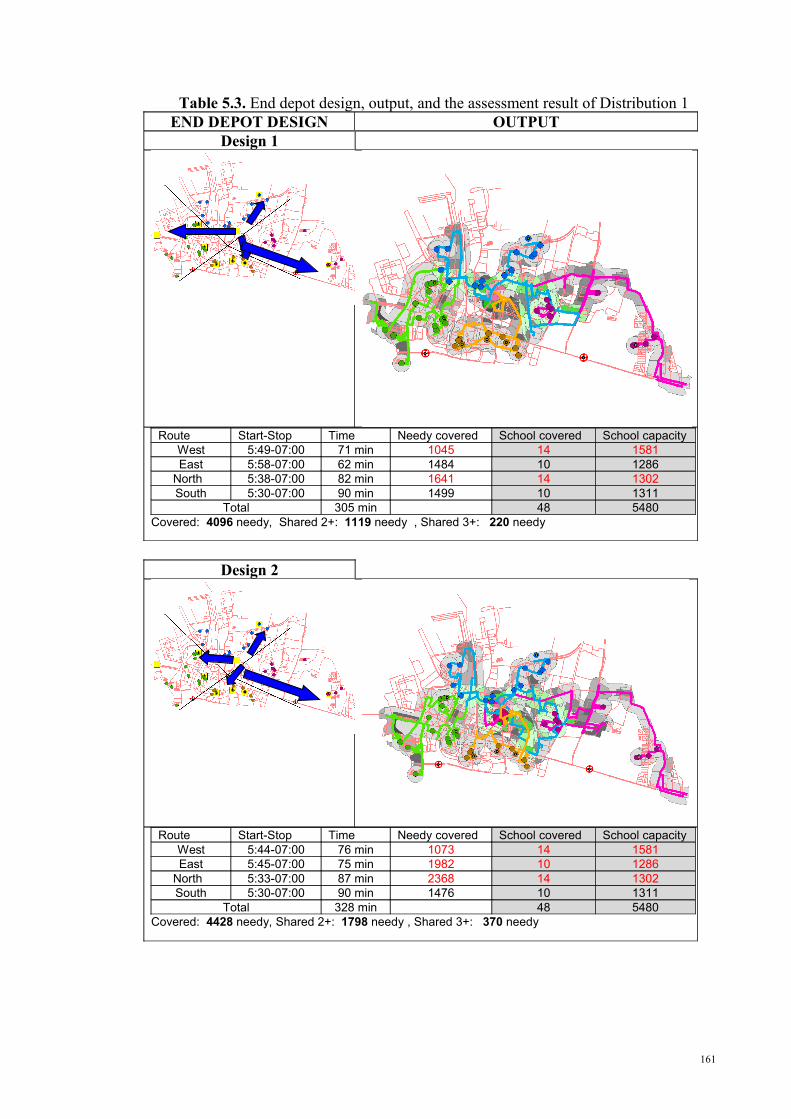
Table 5.3. End depot design, output, and the assessment result of Distribution 1END DEPOT DESIGN OUTPUT

Design 1



Total 305 min 48 5480Covered: 4096 needy, Shared 2+: 1119 needy , Shared 3+: 220 needy

Design 2




161

Design 3




Design 4




162

Table 5.3 shows that although there still appears a lack or excessive are of

covered needy, supervised school areas produce better balance than unsupervised ones.

However, as a consequence, the travel time has seen a significant increase and the total

covered area, in general, has been decreased. This is because the VRP engine must obey

the direction to visit specific schools in each area. In general, this first supervised model

produces a pattern: the west route has excessive school capacities than the covered

needy in its route; in contrast, the north route has a lack of schools with capacity.

Because of this observation, the next distribution design will try to increase the extent

of the west area and decrease the extent of the north area. The new design will resemble

figure 5.9 below.

Figure 5.9. Illustration of second design of school distribution

In this second distribution, west will have 13 schools with needy capacity 1502, the east

10 schools with capacity 1286, the north 10 schools with capacity 854, and the south 15

with capacity 1838. This second design also makes some small changes to the

distribution of available depots. The west area now just has 2 available depots and the

south area has 4 available depots. Following a similar process as with the previous

design, output of this school distribution shows in Table 5.4 below.

163

Table 5.4. End depot design, output, and the assessment result of Distribution 2END DEPOT DESIGN OUTPUT

Design 1



Total 253 min 48 5480Covered : 4252 needy, Shared 2+: 1295 needy , Shared 3+: 281 needy

Design 2




164

Design 3




Design 4



Total 225 min 48 5480Covered : 3868 needy, Shared 2+: 1326 needy , Shared 3+: 300 needy

165

In general, this second design generates better output than the first directed

design. Travel time decreases and the needy are comparable with the same number

capacity. Some needy covered by each route may be in slight excess than the capacity,

but it is not a problem since the routes have sharing areas. Needy in these areas are

counted two or three times for different routes. Some covered needy have to be divided

among the routes, making the actual covered needy less than the covered in each route.

The first assessment point, the route balanced, is passed by all the end depot

designs. The second assessment point is the covered needy. The end depot design 1 can

cover 4252, design 2 can cover 4306, design 3 can cover 4079, and design 4 can cover

3868. The output of design 2 has the most widely covered area. The next position is

design 1. Therefore, in the second assessment point, the candidate design is design 1

and 2. The next point to examine is the time consumed. Design 1 needs 253 minutes

while design 2 needs 266 minutes. The last point, the shared area of design 1, has 1295

needy in that it can choose 2 or more route destinations, while design 2 is 1304. By

comparing these points, design 2 is better in covered area and shared area, while design

2 is better in the time consumed output. Considering the objective of the bus school is

for helping the needy and not taking a profit, then design 2 is chosen. The next section

will detail this chosen route.

If this research is used for another objective, for example for a commercial bus,

it is not impossible that the chosen route is different. It needs to be adjusted between

potential customer (covered area) and the potential cost (time consumed). The

difference of 54 potential passengers may be not worthy spending an additional 13

minutes in the travel time.

166

5.5 The Chosen Route

In the previous section there are several proposed routes that have a good covered

balance. The best choice is the design number 2 in the second school distribution

design. This section will detail this chosen route to give a better understanding before

then continuing with analyzing the route. Figure 5.10 shows these chosen routes.

Figure 5.10 The chosen routes

In tabular view, outputs of routing process are Orders table and Route table.

Orders table shows the detailed sequence and time of arrival and departure of the bus in

each school of each route destination. In the unsupervised Orders route design, each

school will have a certain route name that indicates what route the school is joined,

while in the supervised one this name is already set. The next important value of the

output table is in the Sequence field, ArriveTime field, and DepartTime field that

indicate when the school is visited by the school bus. Another important field is

167

CommuTime field which indicates the total time of the journey of the bus before

stopping at the school. Figure 5.11 shows the output table of the Orders class.

Figure 5.11 Result Table of the Orders class

The chosen route is generated based on the distribution area of the schools in

Figure 5.9. This distribution made the bus must travel across every school in the area

which was in its direction. Buses in the west area need 76 minutes to travel from the

center depot to its last direction. The east route requires 55 minutes, North 60 minutes,

and South 75 minutes. Table 5.5 shows the schools, the route area, the school capacity

and the total capacity of the area, and the detailed minutes when the bus visits them.

168

Table 5.5. Schools visited sequence and timeNo

visit NameRoute Name Minutes Bus Arrived Capacity

1 SMP Wachid Hasyim I east 11 99

2 SMPK. Pecinta Damai east 14 148

3 SMP YP 17 SURABAYA east 17 93

4 SMP Muhammadiyah 15 east 20 132

5 SMP Tri Tunggal VII east 23 97

6 SMP Taruna Jaya I east 34 143

7 SMP Romly Tamim east 46 118

8 SMP PGRI XI east 49 150

9 SMP Negeri 18 east 52 154

10 SMP Terbuka 18 east 54 152 Total capacity east 1286

1 SMP ALKHAIRIYAH north 3 100

2 SMP AL GHOZALI north 6 125

3 SMP AL IRSYAD SURABAYA north 8 115

4 SMP ISLAM AL AMAL north 23 39

5 SMP ISLAM LIL WATHON north 30 41

6 SMP MUHAMMADIYAH 16 north 34 30

7 SMP PGRI VI SBY north 38 110

8 MTs Nurul Salam north 40 13

9 SMP Cahaya north 49 134

10 SMP Negeri 27 north 59 147 Total capacity north 854

1 SMP Muhammadiyah 1 south 13 119

2 SMP Negeri 41 south 16 74

3 SMP YPPI 1 south 28 147

4 SMP Triyasa south 30 148


6 SMP Ganesya I Surabaya south 43 75

7 SMP Katolik Angelus Custos south 48 154

8 SMP GATOTAN 1 SURABAYA south 50 150


10 SMP Ta'miriyah south 55 154

11 SMP Kawung 1 Surabaya south 60 51

12 SMP UNESA 1 SURABAYA south 62 125

13 SMP Bina Bangsa south 65 134

14 SMP Terbuka 5 south 67 149


Total capacity south 1838

1 SMP Gatra west 11 91

2 SMP Negeri 7 west 15 149

3 SMP K St. Mikael west 17 125

4 SMP Al-Ikhlash west 20 149

5 SMP Hang Tuah-4 Surabaya west 22 130

6 SMP PGRI 5 Surabaya west 29 146

7 SMP Islam west 35 72

8 SMP Muhamadiyah XI west 42 95

9 SMP Kemala Bayangkari 6 west 47 112

10 SMP Barunawati west 55 127

11 SMP Mujahidin west 59 109

12 SMP PGRI 36 west 62 12113 SMP Bina Karya west 69 76

Total capacity west 1502

169

For better viewing the routes, Table 5.5 will complement with Figure 5.12, 5.13,

5.14, and 5.15 below. These figures show each route unaccompanied by the others.

While table 5.5 describes the minutes of the arrived bus, these figures describe the

traveling routes.

Figure 5.12 The west route

Figure 5.12 shows that the route begins from the center depot, then it makes a

little rotation in its surrounded area to get the needy. Next, it goes to North West and

visits the first school in 11 minutes. Because every school bus stopped 2 minutes, at 13

minutes it leaves this school. It turns right, and in two minutes comes to the second

school. The second school, third school, fourth school, and fifth school are in a very

short distance from one another. Buses will leave the fifth school at 24 minutes, then go

south in the next 5 minutes, and finally arrives at the sixth school. Going again to the

most south area, the seventh school, it travels in the same way going back to north and

makes a little turn left to visit the eighth school. After turning back the previous way, it

170

is going to the north but takes another street on the right and visits the ninth school. Go

along to the north and the most north school in west area visiting the tenth, the eleventh,

and the twelfth school. It then head to the south again, and visits the thirteenth school

before continuing on to the west depot for a rest.

Figure 5.13 The east route

The west route is complicated, taking a circuitous route back and forth to the

north and south. The east route, shown in Figure 5.13 however is much simpler. The

Bus is just going to the east. In one third of its journey, it visits the first school up to the

fifth school in the contiguous time, because they are a short distance from one another.

After the fifth school, in the second third, it visits the sixth school. Finally, it continues

going to the South East to visit the seventh to tenth schools and ends its journey.

171

Figure 5.14 The north route

The north route, Figure 5.14, is pretty simple too. Starting from the center depot,

the bus goes to the west to collect passengers. It continues to go back to the east and

visit the first, second, and third schools as they lie in a block. Next, in will continue to

the north east to visit the fourth school. Then, turning right to collect more passengers, it

will eventually turn left again to visit the fifth school. Then, going to north and turning

right to visit the sixth, seventh, and eighth schools, it will keep on its journey north to

visit the ninth school. After leaving the ninth school, it heads west to collect passengers.

When it travels back to the tenth school, it remains to rest there to rest.

The south is the last route is the route and contains the most number of schools

and school capacity. The bus will leave the depot and go to the potential needy area in

the southern end of the depot. Going around there first and then continuing its travels,

the bus will be more of south of both the first school and the second school. It continues

to the east to collect passengers again and then back to the west where it visits the third

and fourth schools. Continuing its journey to the west, it turns left in a southern

172

direction to get more passengers, and then back to north to visit the fifth school. The bus

will continue to the north for a while to get passengers and once again head back to the

south and visit the sixth school. The next part of the route has the bus turning right and

going westward. In the middle of its journey west, it visits the seventh to tenth schools.

Continuing from there, it goes to the North West and visits the eleventh to fourteenth

schools. Finally, before the last school which is the fifth school, it goes to the north for

a while to get passengers and then travels back to end its journey. Figure 5.15 shows

this route.

Figure 5.15 The south route

This section has shown the results of the processes that have been explained in the

methodology chapter. By ending this section, this research has completed the routing

stage and will follow with the analyst stage in next section.

173

5.6 Load Analyst Result

In the load analyst process, each route in the Routes class is segmented by

dividing the route per 300 meters. Each segment is then equipped with a necessary field

like those explained in section 4.10.1. There is an AdjLoad field that needs to be filled

in with a calculated and adjusted number of needy surrounding the segment. There is

also an additional Capacity field that will be filled in with the number of school

capacity as in Table 5.5. The table of the result analyst is shown in Figure 5.16 below.

Figure 5.16. Table of the Load analyst

174

TotalLoad, Loss, BackTake, BackLoad, GoTake, and GoLoad fields are filled in

by running the small application in Visual basic with the MapObject2.0 component,

including the programming script that implemented the algorithm in Figure 4.41.

After the calculation step, the result of this load analyst is presented in the 3D

view of ArcScene. There are two types of load that need to be presented here; the load

of the route and the load of inverse route. This 3D is provided with data from the Street

map layer, the Schools, and the needy area map layer. The street layer is presented in 2

dimensional red lines. The school is a point layer and is presented as a big point and the

extruded height shows the value of school capacity. The needy area is also presented as

extruded for the purposes of showing which area has the greatest number of needy

compared with others. With respect to the main data, the route load is presented in two

different layers; the First layer shows the direction route while the second indicates the

inverse route. The directions routes are extruded with the value of GoLoad field while

the inverse with the value of the BackLoad field. Figures 5.17, 5.18, 5.19-5.20, and 5.21

show the 3D representation of the west, east, north, and south routes respectively. It

shows the alteration of passengers in each route, as well as where the potential crowded

areas and lack of passengers will be.

The west route in Figure 5.17 needs an inverse route. This is necessary because

the direction ended at a west depot rather than at a school. So, while traveling to the

west depot, being the end of the journey, the bus still collects needy students. These

passengers need to be picked up and transported in the inverse direction. From the

calculation using the algorithm in Figure 4.41, the West route direction has a maximum

number of 632, while the contra flow is 269. The main direction is colored with green

while the inverse direction is colored with yellow. The maximum number can be seen in

Figure 6.5 and occurs at the start of the journey. The passengers are becoming crowded

while the bus is just beginning the journey. This overcrowding occurs because the bus is

175

going around in an area surrounding the center depot before visiting the first school.

After the bus arrives at several schools, there are still low numbers of passengers until it

finishes its journey.

Figure 5.17. The 3D representation of the passenger load in the west route

Figure 5.18. The 3D representation of the passenger load in the east route

176

In contrast, the east route can be seen in Figure 5.18, and crowds on that route

appear at the end of the journey. In the first third of the journey the passengers are

filling in the groups of schools. Continuing from here into the second third of the route,

there is an excessive passenger load compared with the sixth school capacity. Therefore,

a lot of passengers are still traveling in the last third of the route, and it becomes a

sizeable crowd before arriving at the east group of schools. The maximum number of

passengers on the bus is 761. The East route just requires one way service because a

group of schools resides at the end of the route and fills in the rest of the available bus

space for passengers.

The North route is a bit difficult to see as 3D in one figure. This is because the

main direction and the inverse have a sufficient number of passengers. The difference

from the two other routes is a result of having a school group in the west of the start

depot that has plentiful capacity. This capacity cannot be filled by the short journey in

the west to collect passengers. In the journey to the North East area, a number of

passengers are exceeding the capacity of the schools. The greatest number occurs in the

middle of the North East journey, with the maximum number of needy passengers at

475. Therefore, the inverse route will collect a number of needy in this area. This

inverse route has 248, the maximum number of needy passengers. The needy will travel

until filling in the group of schools in the west of center depot. Figure 5.19 shows the

main direction of the north route while figure 5.20 shows the inverse.

177

Figure 5.19. The 3D representation of the passenger load in the north route; the main direction

Figure 5.20. The 3D representation of the passenger load in the north route; the inverse direction.

The last route, the south, has the most crowded passengers. It followed as the

route with the most capacity and the most covered needy described in the previous

section. The route begins with the bus going around collecting passengers, and collects

a plentiful number for more than one half of the journey. The visited schools cannot

accommodate the needy because on the way to those schools, many passengers also get

onto the bus. The bus is not busy for at last one third of the journey. The South route

178

will need the most number of bus fleets for the main direction, because the maximum

capacity of passengers is 1115, whereas the contra flow needs slightly less because it

has a maximum of 53. Figure 5.21 shows this last route.

Figure 5.21. the 3D representation of the passenger load in the south route

Importantly, this section shows the prediction of the numbers of passengers

which will be loaded in each route. With this prediction, the government can make a

decision regarding how many buses it needs to provide to offer optimum school bus

transportation for its residents which also includes the needy. For example, let’s say, the

bus can carry about 70 needy (50 sitting down and 20 standing). The west route will

need 9 fleets for the main direction and 4 fleets for the inverse. The east route needs 11

buses for its direction while the north route needs more buses in place for the inverse

compared with others. For the main direction it needs 7 fleets and for the inverse it

needs 4 fleets. The south route, which requires 16 fleets, has to provide the most fleets

in the main direction. For accommodating a smaller number of passengers for the

inverse, 1 fleet is enough. These numbers of buses required for optimal bus

transportation may be a great number for the government. However, if at this point

179

these quantities cannot be provided to cover all the needy, the government can still use

this calculated number as a reference for making well-informed decisions regarding

effective distribution of the existing limited number of buses.

5.7 Accessibility Analyst Result

Accessibility analyst result involves calculating the accessibility level of transportation

system media before and after the addition of certain buses. The number of added buses

is taken from the number of buses needed in each route direction and its inverse. First,

to refresh our knowledge about the characteristics of the existing transportation system,

let’s recall the existing transportation system map as shown in Figure 5.22 below.

Figure 5.22 The existing transportation system map

The numbers of buses that need to be provided in each route, then use for

extending the existing transport media. Table 5.6 has been referenced with the existing

transportation system in the section 4.2.6 and the number of bus fleets in the previous

section. It shows the existing transportation media and the added school buses in 4

directions (green background). All transportation media have a number of fleets, a

180

capacity, and the number of secondary school students who use the media. In general,

according to surveys that have been done simultaneously by surveying the existing

transport media in section 4.2.6, the percentage of secondary school students who use

these media in the morning is about 46%. The new provided school bus is especially

applicable for the needy student within this age range. This means the percentage is

100%. This analyst is just derived by using the number of fleet in the morning. Fleets in

the evening are omitted because they have a lot of fleets than in the morning. In other

words, the students who can access transportation media in the morning can also access

it in the evening, but not vice versa. Here, the new school bus is set with a 70 passenger

capacity for the needy. This number is changeable to any number of bus capacities, but

alterations will also make changes in the number of fleet referenced by the maximum

number of passengers while the bus travels from the center depot to each destination,

and the inverse routes mentioned in the previous section. The number of vehicles is

summed from the number of fleets in the main direction and the inverse direction.

Table 5.6. Existing Transport System statistic plus new school bus routes

Route Name Capacity

Number of Vehicle passed % of sec.

school age use

Total number of

Seats05:00 - 07:00 12:00 - 15:00Bus Damri JMP 50 18 56 46% 414Bus Damri Perak 50 27 26 46% 621Lyn C 10 18 60 46% 82Lyn D 10 25 76 46% 115Lyn DA 10 3 49 46% 13Lyn DP 10 23 48 46% 105Lyn IM 10 3 11 46% 13Lyn JMK 10 11 33 46% 50Lyn K 10 97 167 46% 446Lyn LMJ 10 32 41 46% 147Lyn M 10 10 50 46% 46Lyn O 10 34 78 46% 156Lyn Q 10 37 77 46% 170Lyn USP 10 51 106 46% 234Lyn WB 10 6 45 46% 27School Bus North 70 11 11 100% 770School Bus East 70 11 11 100% 770School Bus South 70 17 17 100% 1190School Bus West 70 13 13 100% 910

181

The total number seats value then will be used as the value of the buffer area.

Every buffer area then Sums one to another, with respect to the process model shown in

Figure 4.44. There are two results that are notable: firstly, for the existing transport

system, the sum is therefore ended with the last existing transport media in the above

table (Lyn WB), and secondly the new transport system that continues with adding each

bus route value. The result map is shown in Figures 5.23 and 5.24 below.

Figure 5.23. Accessibility map before school bus was added

The above figure shows the accessibility level in a gradation color of light green

to dark blue to represent the range of accessibility levels from low to high respectively.

From that figure it can be seen that most of region in the study area the one without

color, does not have any accessibility to a transport system. The second position is the

area with the lightest green accessibility level that spreads by the rare transportation

route to west, east, north, and south. This area has an accessibility level which is not

more than 240 points. It means that needy students who live in this area have an

182

opportunity to access seats in the transportation system up to as many as 240. The third

and fourth position is the lightest shades of green respectively that lay in a small part in

the north and center areas.

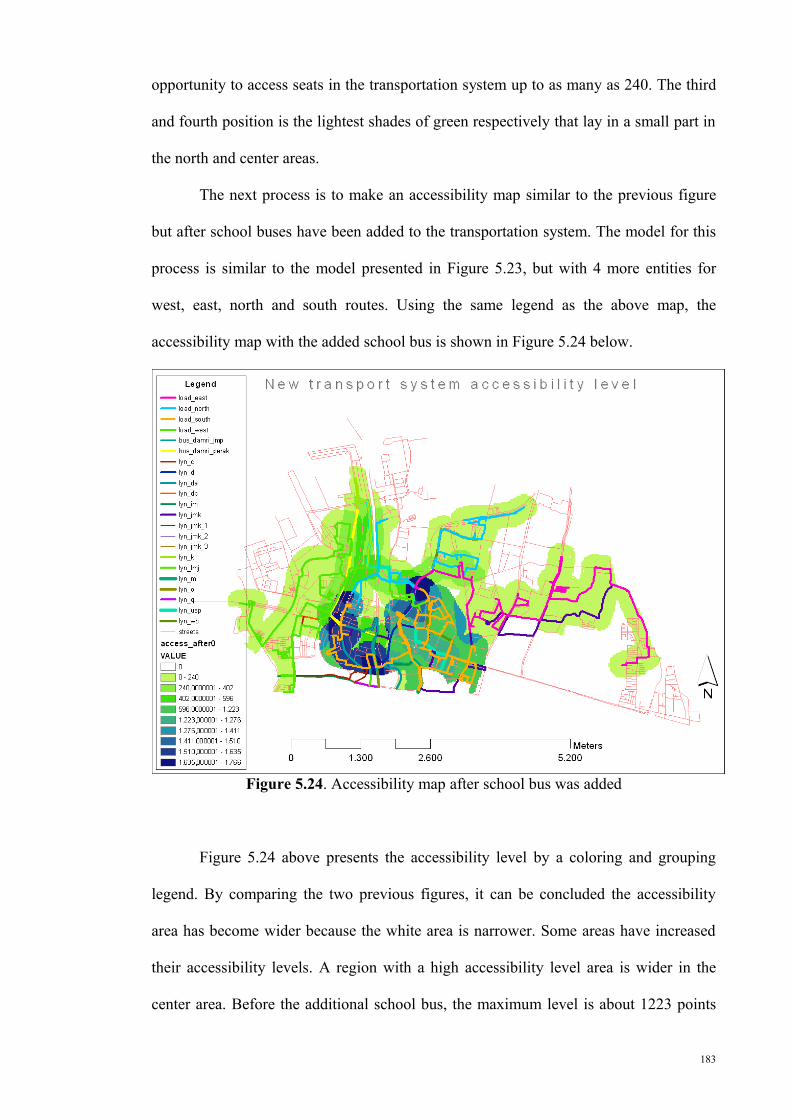
The next process is to make an accessibility map similar to the previous figure

but after school buses have been added to the transportation system. The model for this

process is similar to the model presented in Figure 5.23, but with 4 more entities for

west, east, north and south routes. Using the same legend as the above map, the

accessibility map with the added school bus is shown in Figure 5.24 below.

Figure 5.24. Accessibility map after school bus was added

Figure 5.24 above presents the accessibility level by a coloring and grouping

legend. By comparing the two previous figures, it can be concluded the accessibility

area has become wider because the white area is narrower. Some areas have increased

their accessibility levels. A region with a high accessibility level area is wider in the

center area. Before the additional school bus, the maximum level is about 1223 points

183

which has been presented in green color. Now, after the additional bus, the maximum

level is 1766 which is presented in dark blue color. In this dark blue area, the needy

student has an opportunity to access the transportation fleet with about 1766 seats in the

morning from 05:00 AM to 07:00 AM. This occurs as a result of combining existing

transportation fleet with the school bus fleet.

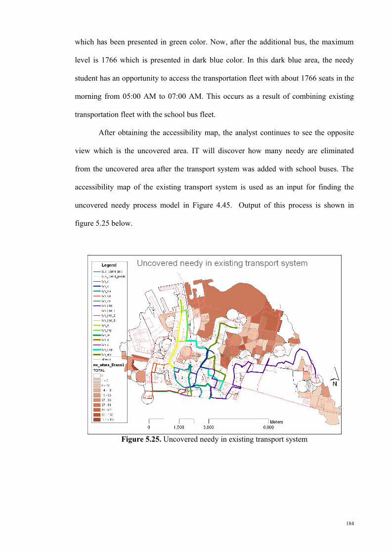
After obtaining the accessibility map, the analyst continues to see the opposite

view which is the uncovered area. IT will discover how many needy are eliminated

from the uncovered area after the transport system was added with school buses. The

accessibility map of the existing transport system is used as an input for finding the

uncovered needy process model in Figure 4.45. Output of this process is shown in

figure 5.25 below.

Figure 5.25. Uncovered needy in existing transport system

184

Following the same process, the accessibility map after the additional school bus

has been added, will be used as input to get the uncovered needy number for the new

transportation system. Figure 5.26 shows this map.

Figure 5.26. Uncovered needy in new transport system

Two figures above have a block map with color similar to the covered needy

map shown in the previous chapter. The difference is that in those maps the gradation

color resides in the area that is far from the street which is used for the transportation

route. The second map has more streets that are included in the transportation route so

the uncovered area is narrower. By calculating the total needy in the remaining area

after cut with the accessibility map, it is found that in the existing transportation system,

the needy number who cannot reach the transport media is 2251 and, after added with

school buses, shrinks to 724 needy children.

185

5.8 Summary

This chapter has shown the result of the processes that have been explained in the

methodology chapter. By ending this chapter, this research has completed the VRP

process and continued with the result of analysis process. This chapter began with the

result of undirected Orders design output, and continued with two kinds of directed

Order design. In each result of different route design and setting is equipped with the

value of assessment process. After comparing this assessment value, the most optimal

route was then chosen. The chosen route then detailed the way to discover the

characteristics of each route destination. After that, this chapter showed how to enhance

the output of VRP process with another geospatial technology. The first enhancement

was to predict the load of passengers in each route destination. This enhancement then

continued this prediction with a calculation of the number of buses that are needed to

run in each route. The second enhancement was to predict the accessibility level of

transportation after a number of buses were added into the transportation system.

Finally, by looking for the opposite area of the accessibility area, the uncovered area

was then discovered.

186

chapter 5 assessing result and analyzing the...

Documents