chapter 4 feature detection and matching - taubin...
TRANSCRIPT

Chapter 4
Feature detection and matching
4.1 Points . . . . . . . . . . . . . . . . . . . . . . . . . . . . . . . . . . . . . . . . . 2134.1.1 Feature detectors . . . . . . . . . . . . . . . . . . . . . . . . . . . . . . . 2154.1.2 Feature descriptors . . . . . . . . . . . . . . . . . . . . . . . . . . . . . . 2284.1.3 Feature matching . . . . . . . . . . . . . . . . . . . . . . . . . . . . . . . 2324.1.4 Feature tracking . . . . . . . . . . . . . . . . . . . . . . . . . . . . . . . 2414.1.5 Application: Performance-driven animation . . . . . . . . . . . . . . . . . 244
4.2 Edges . . . . . . . . . . . . . . . . . . . . . . . . . . . . . . . . . . . . . . . . . 2444.2.1 Edge detection . . . . . . . . . . . . . . . . . . . . . . . . . . . . . . . . 2454.2.2 Edge linking . . . . . . . . . . . . . . . . . . . . . . . . . . . . . . . . . 2554.2.3 Application: Edge editing and enhancement . . . . . . . . . . . . . . . . . 258
4.3 Lines . . . . . . . . . . . . . . . . . . . . . . . . . . . . . . . . . . . . . . . . . 2594.3.1 Successive approximation . . . . . . . . . . . . . . . . . . . . . . . . . . 2604.3.2 Hough transforms . . . . . . . . . . . . . . . . . . . . . . . . . . . . . . . 2604.3.3 Vanishing points . . . . . . . . . . . . . . . . . . . . . . . . . . . . . . . 2654.3.4 Application: Rectangle detection . . . . . . . . . . . . . . . . . . . . . . . 267
4.4 Additional reading . . . . . . . . . . . . . . . . . . . . . . . . . . . . . . . . . . 2694.5 Exercises . . . . . . . . . . . . . . . . . . . . . . . . . . . . . . . . . . . . . . . 269
211

212 Computer Vision: Algorithms and Applications (September 7, 2009 draft)
(a) (b)
(c) (d)
Figure 4.1: A variety of feature detector and descriptors can be used to analyze describe and matchimages: (a) point-like interest operators (Brown et al. 2005); (b) region-like interest operators(Brown et al. 2005); (c) edges (Elder and Golderg 2001); (d) straight lines (Sinha et al. 2008).
4.1. Points 213
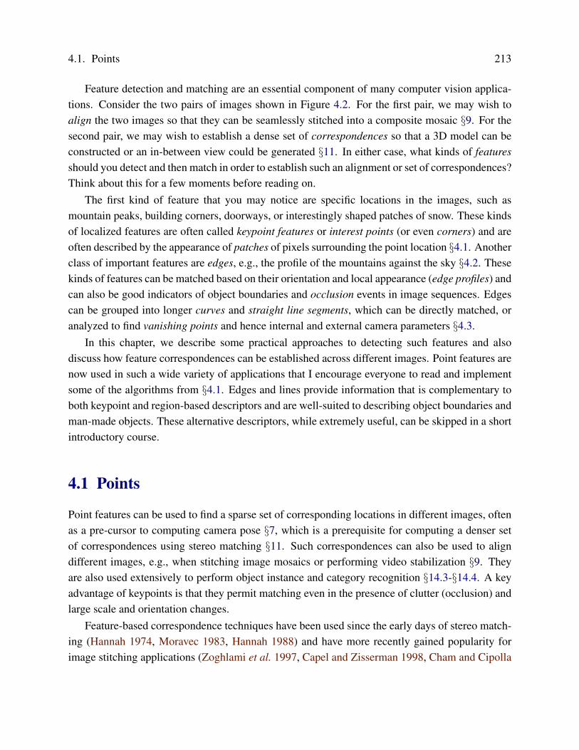
Feature detection and matching are an essential component of many computer vision applica-tions. Consider the two pairs of images shown in Figure 4.2. For the first pair, we may wish toalign the two images so that they can be seamlessly stitched into a composite mosaic §9. For thesecond pair, we may wish to establish a dense set of correspondences so that a 3D model can beconstructed or an in-between view could be generated §11. In either case, what kinds of featuresshould you detect and then match in order to establish such an alignment or set of correspondences?Think about this for a few moments before reading on.
The first kind of feature that you may notice are specific locations in the images, such asmountain peaks, building corners, doorways, or interestingly shaped patches of snow. These kindsof localized features are often called keypoint features or interest points (or even corners) and areoften described by the appearance of patches of pixels surrounding the point location §4.1. Anotherclass of important features are edges, e.g., the profile of the mountains against the sky §4.2. Thesekinds of features can be matched based on their orientation and local appearance (edge profiles) andcan also be good indicators of object boundaries and occlusion events in image sequences. Edgescan be grouped into longer curves and straight line segments, which can be directly matched, oranalyzed to find vanishing points and hence internal and external camera parameters §4.3.
In this chapter, we describe some practical approaches to detecting such features and alsodiscuss how feature correspondences can be established across different images. Point features arenow used in such a wide variety of applications that I encourage everyone to read and implementsome of the algorithms from §4.1. Edges and lines provide information that is complementary toboth keypoint and region-based descriptors and are well-suited to describing object boundaries andman-made objects. These alternative descriptors, while extremely useful, can be skipped in a shortintroductory course.
4.1 Points
Point features can be used to find a sparse set of corresponding locations in different images, oftenas a pre-cursor to computing camera pose §7, which is a prerequisite for computing a denser setof correspondences using stereo matching §11. Such correspondences can also be used to aligndifferent images, e.g., when stitching image mosaics or performing video stabilization §9. Theyare also used extensively to perform object instance and category recognition §14.3-§14.4. A keyadvantage of keypoints is that they permit matching even in the presence of clutter (occlusion) andlarge scale and orientation changes.
Feature-based correspondence techniques have been used since the early days of stereo match-ing (Hannah 1974, Moravec 1983, Hannah 1988) and have more recently gained popularity forimage stitching applications (Zoghlami et al. 1997, Capel and Zisserman 1998, Cham and Cipolla

214 Computer Vision: Algorithms and Applications (September 7, 2009 draft)
Figure 4.2: Two pairs of images to be matched. What kinds of features might one use to establisha set of correspondences between these images?
1998, Badra et al. 1998, McLauchlan and Jaenicke 2002, Brown and Lowe 2007, Brown et al.2005) as well as fully automated 3D modeling (Beardsley et al. 1996, Schaffalitzky and Zisserman2002, Brown and Lowe 2003, Snavely et al. 2006). [ Note: Thin out some of these references? ]
There are two main approaches to finding feature points and their correspondences. The first isto find features in one image that can be accurately tracked using a local search technique such ascorrelation or least squares §4.1.4. The second is to independently detect features in all the imagesunder consideration and then match features based on their local appearance §4.1.3. The former ap-proach is more suitable when images are taken from nearby viewpoints or in rapid succession (e.g.,video sequences), while the latter is more suitable when a large amount of motion or appearancechange is expected, e.g., in stitching together panoramas (Brown and Lowe 2007), establishingcorrespondences in wide baseline stereo (Schaffalitzky and Zisserman 2002), or performing objectrecognition (Fergus et al. 2003).
In this section, we split the keypoint detection and matching pipeline into four separate stages.During the first feature detection (extraction) stage, §4.1.1, each image is searched for locationsthat are likely to match well in other images. At the second feature description stage, §4.1.2, each
4.1. Points 215
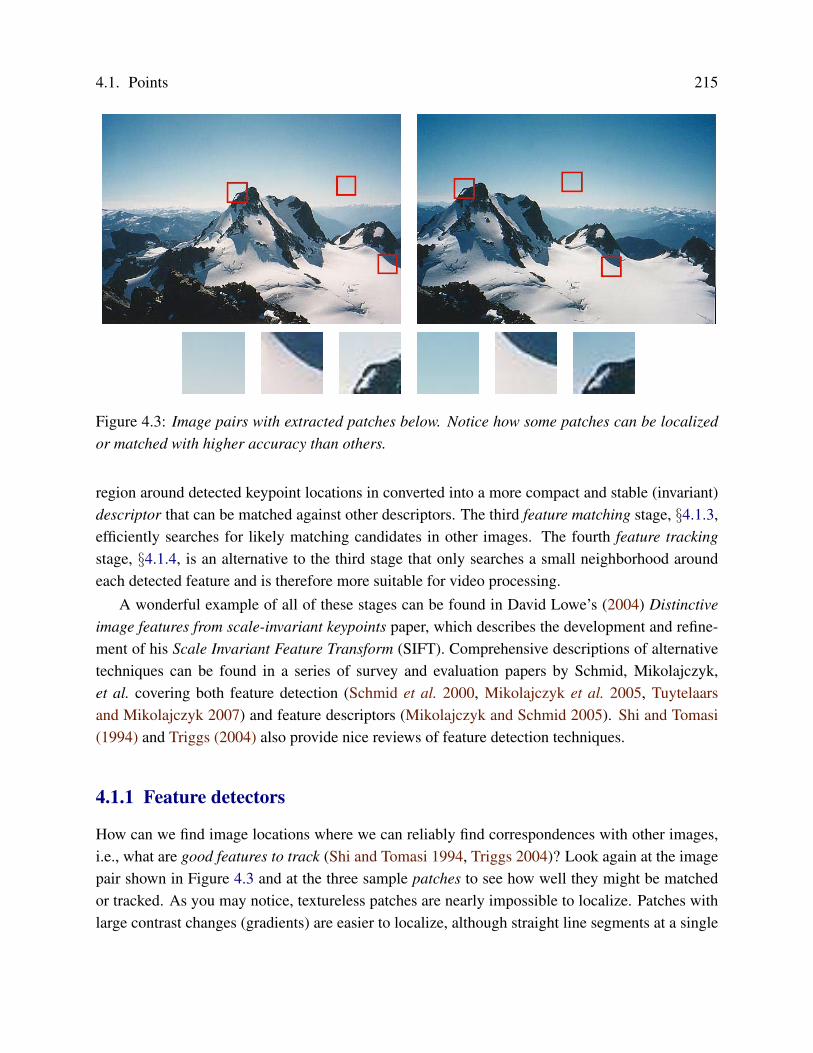
Figure 4.3: Image pairs with extracted patches below. Notice how some patches can be localizedor matched with higher accuracy than others.
region around detected keypoint locations in converted into a more compact and stable (invariant)descriptor that can be matched against other descriptors. The third feature matching stage, §4.1.3,efficiently searches for likely matching candidates in other images. The fourth feature trackingstage, §4.1.4, is an alternative to the third stage that only searches a small neighborhood aroundeach detected feature and is therefore more suitable for video processing.
A wonderful example of all of these stages can be found in David Lowe’s (2004) Distinctiveimage features from scale-invariant keypoints paper, which describes the development and refine-ment of his Scale Invariant Feature Transform (SIFT). Comprehensive descriptions of alternativetechniques can be found in a series of survey and evaluation papers by Schmid, Mikolajczyk,et al. covering both feature detection (Schmid et al. 2000, Mikolajczyk et al. 2005, Tuytelaarsand Mikolajczyk 2007) and feature descriptors (Mikolajczyk and Schmid 2005). Shi and Tomasi(1994) and Triggs (2004) also provide nice reviews of feature detection techniques.
4.1.1 Feature detectors
How can we find image locations where we can reliably find correspondences with other images,i.e., what are good features to track (Shi and Tomasi 1994, Triggs 2004)? Look again at the imagepair shown in Figure 4.3 and at the three sample patches to see how well they might be matchedor tracked. As you may notice, textureless patches are nearly impossible to localize. Patches withlarge contrast changes (gradients) are easier to localize, although straight line segments at a single

216 Computer Vision: Algorithms and Applications (September 7, 2009 draft)
(a) (b) (c)
Figure 4.4: Aperture problems for different image patches: (a) stable (“corner-like”) flow; (b)classic aperture problem (barber-pole illusion); (c) textureless region. The two images I0 (yellow)and I1 (red) are overlaid. The red vector u indicates the displacement between the patch centers,and the w(xi) weighting function (patch window) is shown as a dark circle.
orientation suffer from the aperture problem (Horn and Schunck 1981, Lucas and Kanade 1981,Anandan 1989), i.e., it is only possible to align the patches along the direction normal to the edgedirection (Figure 4.4b). Patches with gradients in at least two (significantly) different orientationsare the easiest to localize, as shown schematically in Figure 4.4a.
These intuitions can be formalized by looking at the simplest possible matching criterion forcomparing two image patches, i.e., their (weighted) summed square difference,
EWSSD(u) =∑
i
w(xi)[I1(xi + u)− I0(xi)]2, (4.1)
where I0 and I1 are the two images being compared, u = (u, v) is the displacement vector, andw(x) is a spatially varying weighting (or window) function. (Note that this is the same formulationwe later use to estimate motion between complete images §8.1, and that this section shares somematerial with that later section.)
When performing feature detection, we do not know which other image location(s) the featurewill end up being matched against. Therefore, we can only compute how stable this metric is withrespect to small variations in position ∆u by comparing an image patch against itself, which isknown as an auto-correlation function or surface
EAC(∆u) =∑
i
w(xi)[I0(xi + ∆u)− I0(xi)]2 (4.2)
(Figure 4.5).1 Note how the auto-correlation surface for the textured flower bed (Figure 4.5b, red1 Strictly speaking, the auto-correlation is the product of the two weighted patches; I’m using the term here in a
more qualitative sense. The weighted sum of squared differences is often called an SSD surface §8.1.

4.1. Points 217
(a)
(b) (c) (d)
Figure 4.5: Three different auto-correlation surfaces (b–d) shown as both grayscale images andsurface plots. The original image (a) is marked with three red crosses to denote where these auto-correlation surfaces were computed. Patch (b) is from the flower bed (good unique minimum),patch (c) is from the roof edge (one-dimensional aperture problem), and patch (d) is from thecloud (no good peak).
218 Computer Vision: Algorithms and Applications (September 7, 2009 draft)
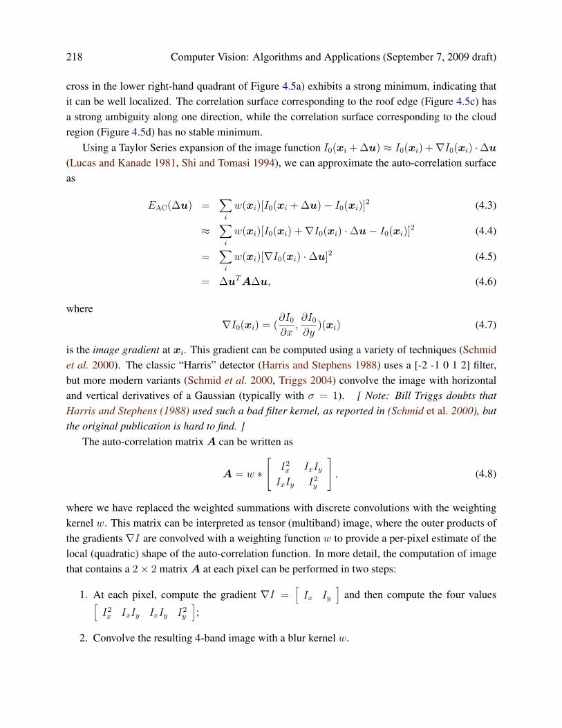
cross in the lower right-hand quadrant of Figure 4.5a) exhibits a strong minimum, indicating thatit can be well localized. The correlation surface corresponding to the roof edge (Figure 4.5c) hasa strong ambiguity along one direction, while the correlation surface corresponding to the cloudregion (Figure 4.5d) has no stable minimum.
Using a Taylor Series expansion of the image function I0(xi + ∆u) ≈ I0(xi) +∇I0(xi) ·∆u(Lucas and Kanade 1981, Shi and Tomasi 1994), we can approximate the auto-correlation surfaceas
EAC(∆u) =∑
i
w(xi)[I0(xi + ∆u)− I0(xi)]2 (4.3)
≈∑
i
w(xi)[I0(xi) +∇I0(xi) ·∆u− I0(xi)]2 (4.4)
=∑
i
w(xi)[∇I0(xi) ·∆u]2 (4.5)
= ∆uTA∆u, (4.6)
where∇I0(xi) = (
∂I0
∂x,∂I0
∂y)(xi) (4.7)
is the image gradient at xi. This gradient can be computed using a variety of techniques (Schmidet al. 2000). The classic “Harris” detector (Harris and Stephens 1988) uses a [-2 -1 0 1 2] filter,but more modern variants (Schmid et al. 2000, Triggs 2004) convolve the image with horizontaland vertical derivatives of a Gaussian (typically with σ = 1). [ Note: Bill Triggs doubts thatHarris and Stephens (1988) used such a bad filter kernel, as reported in (Schmid et al. 2000), butthe original publication is hard to find. ]
The auto-correlation matrixA can be written as
A = w ∗ I2
x IxIyIxIy I2
y
, (4.8)
where we have replaced the weighted summations with discrete convolutions with the weightingkernel w. This matrix can be interpreted as tensor (multiband) image, where the outer products ofthe gradients ∇I are convolved with a weighting function w to provide a per-pixel estimate of thelocal (quadratic) shape of the auto-correlation function. In more detail, the computation of imagethat contains a 2× 2 matrixA at each pixel can be performed in two steps:
1. At each pixel, compute the gradient ∇I =[Ix Iy
]and then compute the four values[
I2x IxIy IxIy I2
y
];
2. Convolve the resulting 4-band image with a blur kernel w.
4.1. Points 219
direction of the slowest change
direction of the fastest change
λ1-1/2
λ0-1/2
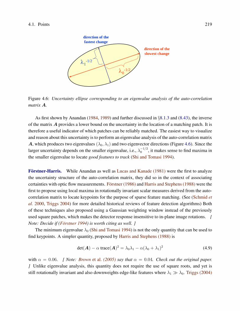
Figure 4.6: Uncertainty ellipse corresponding to an eigenvalue analysis of the auto-correlationmatrixA.
As first shown by Anandan (1984, 1989) and further discussed in §8.1.3 and (8.43), the inverseof the matrixA provides a lower bound on the uncertainty in the location of a matching patch. It istherefore a useful indicator of which patches can be reliably matched. The easiest way to visualizeand reason about this uncertainty is to perform an eigenvalue analysis of the auto-correlation matrixA, which produces two eigenvalues (λ0, λ1) and two eigenvector directions (Figure 4.6). Since thelarger uncertainty depends on the smaller eigenvalue, i.e., λ−1/2
0 , it makes sense to find maxima inthe smaller eigenvalue to locate good features to track (Shi and Tomasi 1994).
Forstner-Harris. While Anandan as well as Lucas and Kanade (1981) were the first to analyzethe uncertainty structure of the auto-correlation matrix, they did so in the context of associatingcertainties with optic flow measurements. Forstner (1986) and Harris and Stephens (1988) were thefirst to propose using local maxima in rotationally invariant scalar measures derived from the auto-correlation matrix to locate keypoints for the purpose of sparse feature matching. (See (Schmid etal. 2000, Triggs 2004) for more detailed historical reviews of feature detection algorithms) Bothof these techniques also proposed using a Gaussian weighting window instead of the previouslyused square patches, which makes the detector response insensitive to in-plane image rotations. [Note: Decide if (Forstner 1994) is worth citing as well. ]
The minimum eigenvalue λ0 (Shi and Tomasi 1994) is not the only quantity that can be used tofind keypoints. A simpler quantity, proposed by Harris and Stephens (1988) is
det(A)− α trace(A)2 = λ0λ1 − α(λ0 + λ1)2 (4.9)
with α = 0.06. [ Note: Brown et al. (2005) say that α = 0.04. Check out the original paper.] Unlike eigenvalue analysis, this quantity does not require the use of square roots, and yet isstill rotationally invariant and also downweights edge-like features where λ1 � λ0. Triggs (2004)

220 Computer Vision: Algorithms and Applications (September 7, 2009 draft)
Figure 4.7: Isocontours of popular keypoint detection functions (Brown et al. 2004). Each detectorlooks for points where the eigenvalues λ0, λ1 ofA = w ∗ ∇I∇IT are both large.
suggest using the quantityλ0 − αλ1 (4.10)
(say with α = 0.05), which also reduces the response at 1D edges, where aliasing errors sometimesinflate the smaller eigenvalue. He also shows how the basic 2 × 2 Hessian can be extended toparametric motions to detect points that are also accurately localizable in scale and rotation. Brownet al. (2005), on the other hand, use the harmonic mean,
det A
tr A=
λ0λ1
λ0 + λ1
, (4.11)
which is a smoother function in the region where λ0 ≈ λ1. Figure 4.7 shows isocontours of thevarious interest point operators (note that all the detectors require both eigenvalues to be large).
[ Note: Decide whether to turn this into a boxed Algorithm. ] The steps in the basic auto-correlation-based keypoint detector can therefore be summarized as follows:
1. Compute the horizontal and vertical derivatives of the image Ix and Iy by convolving theoriginal image with derivatives of Gaussians §3.2.1.
2. Compute the three images corresponding to the outer products of these gradients (the matrixA is symmetric, so only three entries are needed).
3. Convolve each of these images with a larger Gaussian.
4. Compute a scalar interest measure using one of the formulas discussed above.

4.1. Points 221
Note: Sample image Note: Harris response Note: DoG response
(a) (b) (c)
Figure 4.8: Sample image (a) and two different interest operator responses: (b) Harris; (c) DoG.Local maxima are shown as red dots.[ Note: Need to generate this figure. ]
5. Find local maxima above a certain threshold and report these as detected feature point loca-tions.
Figure 4.8 shows the resulting interest operator responses for the classic Harris detector as well asthe DoG detector discussed below.
Adaptive non-maximal suppression While most feature detectors simply look for local maximain the interest function, this can lead to an uneven distribution of feature points across the image,e.g., points will be denser in regions of higher contrast. To mitigate this problem, Brown et al.(2005) only detect features that are both local maxima and whose response value is significantly(10%) greater than than of all of its neighbors within a radius r (Figure 4.9c–d). They devise anefficient way to associate suppression radii with all local maxima by first sorting all local maximaby their response strength, and then creating a second list sorted by decreasing suppression radius(see (Brown et al. 2005) for details). A qualitative comparison of selecting the top n features vs.ANMS is shown in Figure 4.9.
Measuring repeatability Given the large number of feature detectors that have been developedin computer vision, how can we decide which ones to use? Schmid et al. (2000) were the first topropose measuring the repeatability of feature detectors, which is defined as the frequency withwhich keypoints detected in one image are found within ε (say ε = 1.5) pixels of the correspondinglocation in a transformed image. In their paper, they transform their planar images by applyingrotations, scale changes, illumination changes, viewpoint changes, and adding noise. They alsomeasure the information content available at each detected feature point, which they define as theentropy of a set of rotationally invariant local grayscale descriptors. Among the techniques they

222 Computer Vision: Algorithms and Applications (September 7, 2009 draft)
(a) Strongest 250 (b) Strongest 500
(c) ANMS 250, r = 24 (d) ANMS 500, r = 16
Figure 4.9: Adaptive non-maximal suppression (ANMS) (Brown et al. 2005). The two upperimages show the strongest 250 and 500 interest points, while the lower two images show the interestpoints selected with adaptive non-maximal suppression (along with the corresponding suppressionradius r). Note how the latter features have a much more uniform spatial distribution across theimage.
survey, they find that the improved (Gaussian derivative) version of the Harris operator with σd = 1
(scale of the derivative Gaussian) and σi = 2 (scale of the integration Gaussian) works best.
Scale invariance
In many situations, detecting features at the finest stable scale possible may not be appropriate. Forexample, when matching images with little high frequency (e.g., clouds), fine-scale features maynot exist.
One solution to the problem is to extract features at a variety of scales, e.g., by performingthe same operations at multiple resolutions in a pyramid and then matching features at the samelevel. This kind of approach is suitable when the images being matched do not undergo large
4.1. Points 223
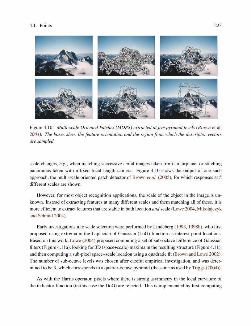
Figure 4.10: Multi-scale Oriented Patches (MOPS) extracted at five pyramid levels (Brown et al.2004). The boxes show the feature orientation and the region from which the descriptor vectorsare sampled.
scale changes, e.g., when matching successive aerial images taken from an airplane, or stitchingpanoramas taken with a fixed focal length camera. Figure 4.10 shows the output of one suchapproach, the multi-scale oriented patch detector of Brown et al. (2005), for which responses at 5different scales are shown.
However, for most object recognition applications, the scale of the object in the image is un-known. Instead of extracting features at many different scales and them matching all of these, it ismore efficient to extract features that are stable in both location and scale (Lowe 2004, Mikolajczykand Schmid 2004).
Early investigations into scale selection were performed by Lindeberg (1993, 1998b), who firstproposed using extrema in the Laplacian of Gaussian (LoG) function as interest point locations.Based on this work, Lowe (2004) proposed computing a set of sub-octave Difference of Gaussianfilters (Figure 4.11a), looking for 3D (space+scale) maxima in the resulting structure (Figure 4.11),and then computing a sub-pixel space+scale location using a quadratic fit (Brown and Lowe 2002).The number of sub-octave levels was chosen after careful empirical investigation, and was deter-mined to be 3, which corresponds to a quarter-octave pyramid (the same as used by Triggs (2004)).
As with the Harris operator, pixels where there is strong asymmetry in the local curvature ofthe indicator function (in this case the DoG) are rejected. This is implemented by first computing

224 Computer Vision: Algorithms and Applications (September 7, 2009 draft)
Scale
(first
octave)
Scale
(next
octave)
Gaussian
Difference of
Gaussian (DOG)
. . .
Figure 1: For each octave of scale space, the initial image is repeatedly convolved with Gaussians toproduce the set of scale space images shown on the left. Adjacent Gaussian images are subtractedto produce the difference-of-Gaussian images on the right. After each octave, the Gaussian image isdown-sampled by a factor of 2, and the process repeated.
In addition, the difference-of-Gaussian function provides a close approximation to thescale-normalized Laplacian of Gaussian, σ2∇2G, as studied by Lindeberg (1994). Lindebergshowed that the normalization of the Laplacian with the factor σ2 is required for true scaleinvariance. In detailed experimental comparisons, Mikolajczyk (2002) found that the maximaand minima of σ2∇2G produce the most stable image features compared to a range of otherpossible image functions, such as the gradient, Hessian, or Harris corner function.
The relationship between D and σ2∇2G can be understood from the heat diffusion equa-tion (parameterized in terms of σ rather than the more usual t = σ2):
∂G
∂σ= σ∇2G.
From this, we see that ∇2G can be computed from the finite difference approximation to∂G/∂σ, using the difference of nearby scales at kσ and σ:
σ∇2G =∂G
∂σ≈ G(x, y, kσ) −G(x, y, σ)
kσ − σ
and therefore,
G(x, y, kσ) −G(x, y, σ) ≈ (k − 1)σ2∇2G.
This shows that when the difference-of-Gaussian function has scales differing by a con-stant factor it already incorporates the σ2 scale normalization required for the scale-invariant
6
Scale
Figure 2: Maxima and minima of the difference-of-Gaussian images are detected by comparing apixel (marked with X) to its 26 neighbors in 3x3 regions at the current and adjacent scales (markedwith circles).
Laplacian. The factor (k − 1) in the equation is a constant over all scales and therefore doesnot influence extrema location. The approximation error will go to zero as k goes to 1, butin practice we have found that the approximation has almost no impact on the stability ofextrema detection or localization for even significant differences in scale, such as k =
√2.
An efficient approach to construction of D(x, y, σ) is shown in Figure 1. The initialimage is incrementally convolved with Gaussians to produce images separated by a constantfactor k in scale space, shown stacked in the left column. We choose to divide each octaveof scale space (i.e., doubling of σ) into an integer number, s, of intervals, so k = 21/s.We must produce s + 3 images in the stack of blurred images for each octave, so that finalextrema detection covers a complete octave. Adjacent image scales are subtracted to producethe difference-of-Gaussian images shown on the right. Once a complete octave has beenprocessed, we resample the Gaussian image that has twice the initial value of σ (it will be 2images from the top of the stack) by taking every second pixel in each row and column. Theaccuracy of sampling relative to σ is no different than for the start of the previous octave,while computation is greatly reduced.
3.1 Local extrema detection
In order to detect the local maxima and minima of D(x, y, σ), each sample point is comparedto its eight neighbors in the current image and nine neighbors in the scale above and below(see Figure 2). It is selected only if it is larger than all of these neighbors or smaller than allof them. The cost of this check is reasonably low due to the fact that most sample points willbe eliminated following the first few checks.
An important issue is to determine the frequency of sampling in the image and scale do-mains that is needed to reliably detect the extrema. Unfortunately, it turns out that there isno minimum spacing of samples that will detect all extrema, as the extrema can be arbitrar-ily close together. This can be seen by considering a white circle on a black background,which will have a single scale space maximum where the circular positive central region ofthe difference-of-Gaussian function matches the size and location of the circle. For a veryelongated ellipse, there will be two maxima near each end of the ellipse. As the locations ofmaxima are a continuous function of the image, for some ellipse with intermediate elongationthere will be a transition from a single maximum to two, with the maxima arbitrarily close to
7
(a) (b)
Figure 4.11: Scale-space feature detection using a sub-octave Difference of Gaussian pyramid(Lowe 2004). (a) Adjacent levels of a sub-octave Gaussian pyramid are subtracted to produceDifference of Gaussian images. (b) Extrema (maxima and minima) in the resulting 3D volume aredetected by comparing a pixel to its 26 neighbors.
the local Hessian of the difference image D,
H =
Dxx Dxy
Dxy Dyy
, (4.12)
and then rejecting keypoints for which
Tr(H)2
Det(H)> 10. (4.13)
While Lowe’s Scale Invariant Feature Transform (SIFT) performs well in practice, it is notbased on the same theoretical foundation of maximum spatial stability as the auto-correlation-based detectors. (In fact, its detection locations are often complementary to those produced bysuch techniques and can therefore be used in conjunction with these other approaches.) In orderto add a scale selection mechanism to the Harris corner detector, Mikolajczyk and Schmid (2004)evaluate the Laplacian of a Gaussian function at each detected Harris point (in a multi-scale pyra-mid) and keep only those points for which the Laplacian is extremal (larger or smaller than bothits coarser and finer-level values). An optional iterative refinement for both scale and position isalso proposed and evaluated. Additional examples of scale invariant region detectors can be foundin (Mikolajczyk et al. 2005, Tuytelaars and Mikolajczyk 2007).
4.1. Points 225
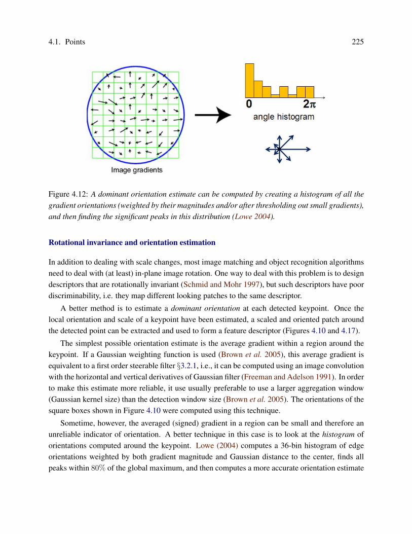
Figure 4.12: A dominant orientation estimate can be computed by creating a histogram of all thegradient orientations (weighted by their magnitudes and/or after thresholding out small gradients),and then finding the significant peaks in this distribution (Lowe 2004).
Rotational invariance and orientation estimation
In addition to dealing with scale changes, most image matching and object recognition algorithmsneed to deal with (at least) in-plane image rotation. One way to deal with this problem is to designdescriptors that are rotationally invariant (Schmid and Mohr 1997), but such descriptors have poordiscriminability, i.e. they map different looking patches to the same descriptor.
A better method is to estimate a dominant orientation at each detected keypoint. Once thelocal orientation and scale of a keypoint have been estimated, a scaled and oriented patch aroundthe detected point can be extracted and used to form a feature descriptor (Figures 4.10 and 4.17).
The simplest possible orientation estimate is the average gradient within a region around thekeypoint. If a Gaussian weighting function is used (Brown et al. 2005), this average gradient isequivalent to a first order steerable filter §3.2.1, i.e., it can be computed using an image convolutionwith the horizontal and vertical derivatives of Gaussian filter (Freeman and Adelson 1991). In orderto make this estimate more reliable, it use usually preferable to use a larger aggregation window(Gaussian kernel size) than the detection window size (Brown et al. 2005). The orientations of thesquare boxes shown in Figure 4.10 were computed using this technique.
Sometime, however, the averaged (signed) gradient in a region can be small and therefore anunreliable indicator of orientation. A better technique in this case is to look at the histogram oforientations computed around the keypoint. Lowe (2004) computes a 36-bin histogram of edgeorientations weighted by both gradient magnitude and Gaussian distance to the center, finds allpeaks within 80% of the global maximum, and then computes a more accurate orientation estimate
226 Computer Vision: Algorithms and Applications (September 7, 2009 draft)
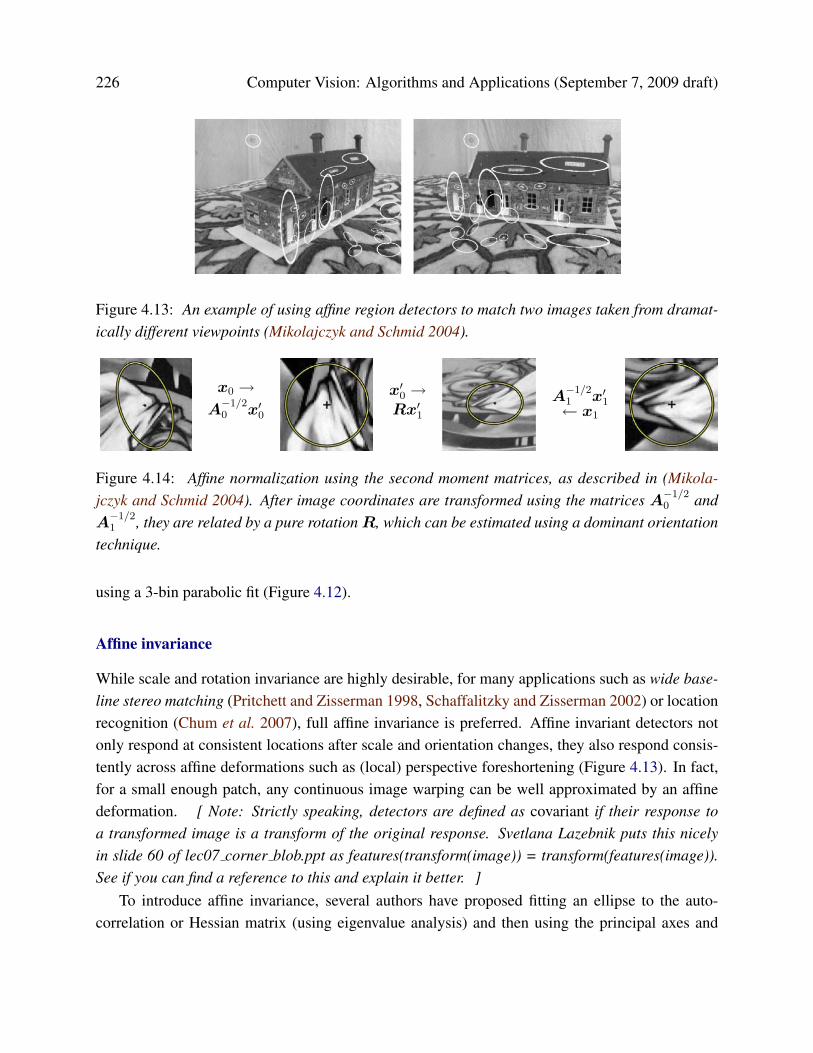
Figure 4.13: An example of using affine region detectors to match two images taken from dramat-ically different viewpoints (Mikolajczyk and Schmid 2004).
x0 →A−1/20 x′0
x′0 →Rx′1
A−1/21 x′1← x1
Figure 4.14: Affine normalization using the second moment matrices, as described in (Mikola-jczyk and Schmid 2004). After image coordinates are transformed using the matrices A−1/2
0 andA−1/21 , they are related by a pure rotationR, which can be estimated using a dominant orientation
technique.
using a 3-bin parabolic fit (Figure 4.12).
Affine invariance
While scale and rotation invariance are highly desirable, for many applications such as wide base-line stereo matching (Pritchett and Zisserman 1998, Schaffalitzky and Zisserman 2002) or locationrecognition (Chum et al. 2007), full affine invariance is preferred. Affine invariant detectors notonly respond at consistent locations after scale and orientation changes, they also respond consis-tently across affine deformations such as (local) perspective foreshortening (Figure 4.13). In fact,for a small enough patch, any continuous image warping can be well approximated by an affinedeformation. [ Note: Strictly speaking, detectors are defined as covariant if their response toa transformed image is a transform of the original response. Svetlana Lazebnik puts this nicelyin slide 60 of lec07 corner blob.ppt as features(transform(image)) = transform(features(image)).See if you can find a reference to this and explain it better. ]
To introduce affine invariance, several authors have proposed fitting an ellipse to the auto-correlation or Hessian matrix (using eigenvalue analysis) and then using the principal axes and

4.1. Points 227
Figure 4.15: Maximally Stable Extremal Regions (MSERs) extracted and matched from a numberof images (Matas et al. 2004).
ratios of this fit as the affine coordinate frame (Lindeberg and Gøarding 1997, Baumberg 2000,Mikolajczyk and Schmid 2004, Mikolajczyk et al. 2005, Tuytelaars and Mikolajczyk 2007). Fig-ure 4.14 shows how the square root of the moment matrix can be use to transform local patchesinto a frame which is similar up to rotation. [ Note: May need to fix up the above description. ]
Another important affine invariant region detector is the Maximally Stable Extremal Region(MSER) detector developed by Matas et al. (2004). To detect MSERs, binary regions are com-puted by thresholding the image at all possible gray levels (the technique therefore only worksfor grayscale images). This can be performed efficiently by first sorting all pixels by gray value,and then incrementally adding pixels to each connected component as the threshold is changed(Nister and Stewenius 2008). The area of each component (region) is monitored as the threshold ischanged. Regions whose rate of change of area w.r.t. threshold is minimal are defined as maximallystable and are returned as detected regions. This results in regions that are invariant to both affinegeometric and photometric (linear bias-gain or smooth monotonic) transformations (Figure 4.15).If desired, an affine coordinate frame can be fit to each detected region using its moment matrix.
The area of feature point detectors and descriptors continues to be very active, with papersappearing every year at major computer vision conferences (Xiao and Shah 2003, Koethe 2003,Carneiro and Jepson 2005, Kenney et al. 2005, Bay et al. 2006, Platel et al. 2006, Rosten andDrummond 2006). Mikolajczyk et al. (2005) survey a number of popular affine region detectorsand provide experimental comparisons of their invariance to common image transformations suchas scaling, rotations, noise, and blur. These experimental results, code, and pointers to the surveyedpapers can be found on their Web site at http://www.robots.ox.ac.uk/vgg/research/affine.
[ Note: Clean up the rest of this section. Can I get some suggestions from reviewers as towhich are most important? ] Of course, keypoints are not the only kind of features that can beused for registering images. Zoghlami et al. (1997) use line segments as well as point-like featuresto estimate homographies between pairs of images, whereas (Bartoli et al. 2004) use line segmentswith local correspondences along the edges to extract 3D structure and motion. [ Note: Check out(Schmid and Zisserman 1997) and see what they do. ] Tuytelaars and Van Gool (2004) use affineinvariant regions to detect correspondences for wide baseline stereo matching, whereas Kadir et

228 Computer Vision: Algorithms and Applications (September 7, 2009 draft)
Figure 4.16: Feature matching: how can we extract local descriptors that are invariant to inter-image variations and yet still discriminative enough to establish correct correspondences?
al. (2004) detect salient regions where patch entropy and its rate of change with scale are locallymaximal. (Corso and Hager (2005) use a related technique to fit 2D oriented Gaussian kernels tohomogeneous regions.) [ Note: The following text is from Matas’ BMVC 2002 paper: Since the
influential paper by Schmid and Mohr [11] many image matching and wide-baseline stereo algorithms have
been proposed, most commonly using Harris interest points as distinguished regions. Tell and Carlsson [13]
proposed a method where line segments connecting Harris interest points form measurement regions. The
measurements are characterized by scale invariant Fourier coefficients. The Harris interest detector is stable
over a range of scales, but defines no scale or affine invariant measurement region. Baumberg [1] applied an
iterative scheme originally proposed by Lindeberg and Garding to associate affine-invariant measurement
regions with Harris interest points. In [7], Mikolajczyk and Schmid show that a scale-invariant MR can
be found around Harris interest points. In [9], Pritchett and Zisserman form groups of line segments and
estimate local homographies using parallelograms as measurement regions. Tuytelaars and Van Gool intro-
duced two new classes of affine-invariant distinguished regions, one based on local intensity extrema [16]
the other using point and curve features [15]. In the latter approach, DRs are characterized by measurements
from inside an ellipse, constructed in an affine invariant manner. Lowe [6] describes the “Scale Invariant
Feature Transform” approach which produces a scale and orientation-invariant characterization of interest
points. ]More details on techniques for finding and matching curves, lines, and regions, can be found
in subsequent sections of this chapter.
4.1.2 Feature descriptors
After detecting the features (keypoints), we must match them, i.e., determine which features comefrom corresponding locations in different images. In some situations, e.g., for video sequences(Shi and Tomasi 1994) or for stereo pairs that have been rectified (Zhang et al. 1995, Loop andZhang 1999, Scharstein and Szeliski 2002), the local motion around each feature point may bemostly translational. In this case, the simple error metrics such as the sum of squared differencesor normalized cross-correlation, described in §8.1, can be used to directly compare the intensities

4.1. Points 229
Figure 4.17: MOPS descriptors are formed using an 8 × 8 sampling of bias/gain normalizedintensity values, with a sample spacing of 5 pixels relative to the detection scale (Brown et al.2005). This low frequency sampling gives the features some robustness to interest point locationerror, and is achieved by sampling at a higher pyramid level than the detection scale.
in small patches around each feature point. (The comparative study by Mikolajczyk and Schmid(2005) discussed below uses cross-correlation.) Because feature points may not be exactly located,a more accurate matching score can be computed by performing incremental motion refinement asdescribed in §8.1.3, but this can be time consuming and can sometimes even decrease performance(Brown et al. 2005).
In most cases, however, the local appearance of features will change in orientation, scale,and even affine frame between images. Extracting a local scale, orientation, and/or affine frameestimate and then using this to resample the patch before forming the feature descriptor is thususually preferable (Figure 4.17).
Even after compensating for these changes, the local appearance of image patches will usuallystill vary from image to image. How can we make the descriptor that we match more invari-ant to such changes, while still preserving discriminability between different (non-corresponding)patches (Figure 4.16)? Mikolajczyk and Schmid (2005) review some recently developed view-invariant local image descriptors and experimentally compare their performance. Below, we de-scribe a few of these descriptor in more detail.
Bias and gain normalization (MOPS). For tasks that do not exhibit large amounts of foreshort-ening, such as image stitching, simple normalized intensity patches perform reasonably well andare simple to implement (Brown et al. 2005) (Figure 4.17). In order to compensate for slight inac-curacies in the feature point detector (location, orientation, and scale), these Multi-Scale OrientedPatches (MOPS) are sampled at spacing of 5 pixels relative to the detection scale (using a coarserlevel of the image pyramid to avoid aliasing). To compensate for affine photometric variations (lin-ear exposure changes, aka bias and gain, (3.3)), patch intensities are re-scaled so that their mean iszero and their variance is one.

230 Computer Vision: Algorithms and Applications (September 7, 2009 draft)
Figure 4.18: A schematic representation of Lowe’s (2004) Scale Invariant Feature Transform(SIFT). Gradient orientations and magnitudes are computed at each pixel and then weighted by aGaussian falloff (blue circle). A weighted gradient orientation histogram is then computed in eachsubregion, using trilinear interpolation. While this figure shows an 8 × 8 pixel patch and a 2 × 2
descriptor array, Lowe’s actual implementation uses 16 × 16 patches and a 4 × 4 array of 8-binhistograms.
Scale Invariant Feature Transform (SIFT). SIFT features are formed by computing the gradi-ent at each pixel in a 16 × 16 window around the detected keypoint, using the appropriate levelof the Gaussian pyramid at which the keypoint was detected. The gradient magnitudes are down-weighted by a Gaussian fall-off function (shown as a blue circle), in order to reduce the influenceof gradients far from the center, as these are more affected by small misregistrations (Figure 4.18).
In each 4×4 quadrant, a gradient orientation histogram is formed by (conceptually) adding theweighted gradient value to one of 8 orientation histogram bins. To reduce the effects of locationand dominant orientation misestimation, each of the original 256 weighted gradient magnitudes issoftly added to 2 × 2 × 2 histogram bins using trilinear interpolation. (Softly distributing valuesto adjacent histogram bins is generally a good idea in any application where histograms are beingcomputed, e.g., for Hough transforms §4.3.2 or local histogram equalization §3.1.4.
The resulting 128 non-negative values form a raw version of the SIFT descriptor vector. Toreduce the effects of contrast/gain (additive variations are already removed by the gradient), the128-D vector is normalized to unit length. To further make the descriptor robust to other photo-metric variations, values are clipped to 0.2 and the resulting vector is once again renormalized tounit length.
PCA-SIFT Ke and Sukthankar (2004) propose a (simpler to compute) descriptor inspired by

4.1. Points 231
Figure 4.19: The Gradient Location-Orientation Histogram (GLOH) descriptor uses log-polarbins instead of square bins to compute orientation histograms (Mikolajczyk and Schmid 2005).[ Note: No need to get permission for this figure, I drew it myself. ]
SIFT, which computes the x and y (gradient) derivatives over a 39 × 39 patch and then reducesthe resulting 3042-dimensional vector to 36 using PCA (Principal Component Analysis) §14.1.1,§A.1.2.
Gradient location-orientation histogram (GLOH) This descriptor, developed by Mikolajczykand Schmid (2005), is a variant on SIFT that uses a log-polar binning structure instead of the 4quadrants used by Lowe (2004) (Figure 4.19). The spatial bins are of radius 6, 11, and 15, witheight angular bins (except for the central region), for a total of 17 spatial bins and 16 orientationbins. The 272-dimensional histogram is then projected onto a 128 dimensional descriptor usingPCA trained on a large database. In their evaluation, Mikolajczyk and Schmid (2005) found thatGLOH, which has the best performance overall, outperforms SIFT by a small margin.
Steerable filters Steerable filters, §3.2.1, are combinations of derivative of Gaussian filters thatpermit the rapid computation of even and odd (symmetric and anti-symmetric) edge-like andcorner-like features at all possible orientations (Freeman and Adelson 1991). Because they usereasonably broad Gaussians, they too are somewhat insensitive to localization and orientation er-rors.
Performance of local descriptors Among the local descriptors that Mikolajczyk and Schmid(2005) compared, they found that GLOH performed the best, followed closely by SIFT (Fig-ure 4.25). Results for many other descriptors, not covered in this book, are also presented.

232 Computer Vision: Algorithms and Applications (September 7, 2009 draft)
(a) (b)
Figure 4.20: Spatial summation blocks for SIFT, GLOH, and some newly developed feature de-scriptors (Winder and Brown 2007). The parameters for the new features (a), e.g., their Gaussianweights, are learned from a training database of matched real-world image patches (b) obtainedfrom robust structure-from-motion applied to Internet photo collections (Hua et al. 2007, Snavelyet al. 2006).
The field of feature descriptors continues to evolve rapidly, with some of the newer techniqueslooking at local color information (van de Weijer and Schmid 2006, Abdel-Hakim and Farag 2006).Winder and Brown (2007) develop a multi-stage framework for feature descriptor computation thatsubsumes both SIFT and GLOH (Figure 4.20a) and also allows them to learn optimal parametersfor newer descriptors that outperform previous hand-tuned descriptors. Hua et al. (2007) extendthis work by learning lower-dimensional projections of higher-dimensional descriptors that havethe best discriminative power. Both of these papers use a database of real-world image patches(Figure 4.20b) obtained by sampling images at locations that were reliably matched using a robuststructure-from-motion algorithm applied to Internet photo collections (Snavely et al. 2006, Goeseleet al. 2007).
While these techniques construct feature detectors that optimize for repeatability across all ob-ject classes, it is also possible to develop class- or instance-specific feature detectors that maximizediscriminability from other classes (Ferencz et al. 2008).
4.1.3 Feature matching
Once we have extracted features and their descriptors from two or more images, the next step is toestablish some preliminary feature matches between these images. The approach we take dependspartially on the application, e.g., different strategies may be preferable for matching images that areknown to overlap (e.g., in image stitching) vs. images that may have no correspondence whatsoever(e.g., when trying to recognize objects from a database).
In this section, we divide this problem into two separate components. The first is to select amatching strategy, which determines which correspondences are passed on to the next stage forfurther processing. The second is to devise efficient data structures and algorithms to perform

4.1. Points 233
Figure 4.21: Recognizing objects in a cluttered scene (Lowe 2004). Two of the training images inthe database are shown on the left. These are matched to the cluttered scene in the middle usingSIFT features, shown as small squares in the right image. The affine warp of each recognizeddatabase image onto the scene is shown as a larger parallelogram in the right image.
this matching as quickly as possible. (See the discussion of related techniques in the chapter onrecognition §14.3.2.)
Matching strategy and error rates
As we mentioned before, the determining which features matches are reasonable to further processdepends on the context in which the matching is being performed. Say we are given two imagesthat overlap to a fair amount (e.g., for image stitching, as in Figure 4.16, or for tracking objects ina video). We know that most features in one image are likely to match the other image, althoughsome may not match because they are occluded or their appearance has changed too much.
On the other hand, if we are trying to recognize how may known objects appear in a clutteredscene (Figure 4.21), most of the features may not match. Furthermore, a large number of poten-tially matching objects must be searched, which requires more efficient strategies, as describedbelow.
To begin with, we assume that the feature descriptors have been designed so that Euclidean(vector magnitude) distances in feature space can be used for ranking potential matches. If itturns out that certain parameters (axes) in a descriptor are more reliable than others, it is usuallypreferable to re-scale these axes ahead of time, e.g., by determining how much they vary whencompared against other known good matches (Hua et al. 2007). (A more general process thatinvolves transforming feature vectors into a new scaled basis is called whitening, and is discussedin more detail in the context of eigenface-based face recognition §14.1.1 (14.7).)
Given a Euclidean distance metric, the simplest matching strategy is to set a threshold (max-

234 Computer Vision: Algorithms and Applications (September 7, 2009 draft)
11
2
1
3
4
Figure 4.22: An example of false positives and negatives. The black digits 1 and 2 are the featuresbeing matched against a database of features in other images. At the current threshold setting(black circles), the green 1 is a true positive (good match), the blue 1 is a false negative (failure tomatch), and the red 3 is a false positive (incorrect match). If we set the threshold higher (dashedcircle), the blue 1 becomes a true positive, but the brown 4 becomes an additional false positive.
imum distance) and to return all matches from other images within this threshold. Setting thethreshold too high results in too many false positives, i.e., incorrect matches being returned. Set-ting the threshold too low results in too many false negatives, i.e., too many correct matches beingmissed (Figure 4.22).
We can quantify the performance of a matching algorithm at a particular threshold by firstcounting the number of true and false matches and match failures, using the following definitions(Fawcett 2006):
• TP: true positives, i.e., number of correct matches;
• FN: false negatives, matches that were not correctly detected;
• FP: false positives, estimated matches that are incorrect;
• TN: true negatives, non-matches that were correctly rejected.
Table 4.1 shows a sample confusion matrix (contingency table) containing such numbers.We can convert these numbers into unit rates by defining the following quantities (Fawcett
2006):
• true positive rate TPR,
TPR =TP
TP+FN=
TPP
; (4.14)
• false positive rate FPR,
FPR =FP
FP+TN=
FPN
; (4.15)
4.1. Points 235
.True matches True non-matchPred. matches TP = 18 FP = 4 P' = 22 PPV = 0.82Pred. non-match. FN = 2 TN = 76 N' = 78
P = 20 N = 80 Total = 100
TPR = 0.90 FPR = 0.05 ACC = 0.94
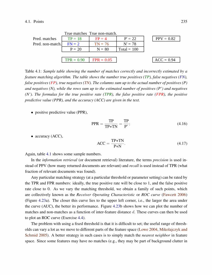
Table 4.1: Sample table showing the number of matches correctly and incorrectly estimated by afeature matching algorithm. The table shows the number true positives (TP), false negatives (FN),false positives (FP), true negatives (TN). The columns sum up to the actual number of positives (P)and negatives (N), while the rows sum up to the estimated number of positives (P’) and negatives(N’). The formulas for the true positive rate (TPR), the false positive rate (FPR), the positivepredictive value (PPR), and the accuracy (ACC) are given in the text.
• positive predictive value (PPR),
PPR =TP
TP+TN=
TPP’
; (4.16)
• accuracy (ACC),
ACC =TP+TN
P+N. (4.17)
Again, table 4.1 shows some sample numbers.In the information retrieval (or document retrieval) literature, the terms precision is used in-
stead of PPV (how many returned documents are relevant) and recall is used instead of TPR (whatfraction of relevant documents was found).
Any particular matching strategy (at a particular threshold or parameter setting) can be rated bythe TPR and FPR numbers: ideally, the true positive rate will be close to 1, and the false positiverate close to 0. As we vary the matching threshold, we obtain a family of such points, whichare collectively known as the Receiver Operating Characteristic or ROC curve (Fawcett 2006)(Figure 4.23a). The closer this curve lies to the upper left corner, i.e., the larger the area underthe curve (AUC), the better its performance. Figure 4.23b shows how we can plot the number ofmatches and non-matches as a function of inter-feature distance d. These curves can then be usedto plot an ROC curve (Exercise 4.4).
The problem with using a fixed threshold is that it is difficult to set; the useful range of thresh-olds can vary a lot as we move to different parts of the feature space (Lowe 2004, Mikolajczyk andSchmid 2005). A better strategy in such cases is to simply match the nearest neighbor in featurespace. Since some features may have no matches (e.g., they may be part of background clutter in
236 Computer Vision: Algorithms and Applications (September 7, 2009 draft)
false positive rate
true
posi
tive
rate
0.1
0.8
0 1
1
equal error
rate
random chance
TPFP FN
TN
θ d
#
(a) (b)
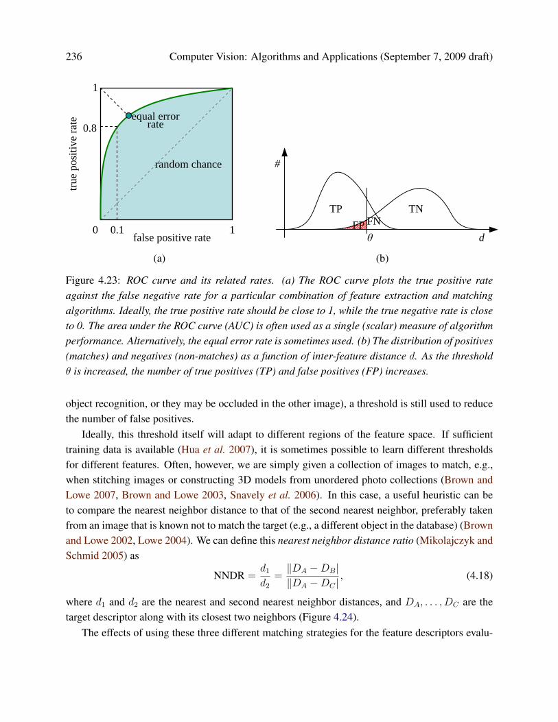
Figure 4.23: ROC curve and its related rates. (a) The ROC curve plots the true positive rateagainst the false negative rate for a particular combination of feature extraction and matchingalgorithms. Ideally, the true positive rate should be close to 1, while the true negative rate is closeto 0. The area under the ROC curve (AUC) is often used as a single (scalar) measure of algorithmperformance. Alternatively, the equal error rate is sometimes used. (b) The distribution of positives(matches) and negatives (non-matches) as a function of inter-feature distance d. As the thresholdθ is increased, the number of true positives (TP) and false positives (FP) increases.
object recognition, or they may be occluded in the other image), a threshold is still used to reducethe number of false positives.
Ideally, this threshold itself will adapt to different regions of the feature space. If sufficienttraining data is available (Hua et al. 2007), it is sometimes possible to learn different thresholdsfor different features. Often, however, we are simply given a collection of images to match, e.g.,when stitching images or constructing 3D models from unordered photo collections (Brown andLowe 2007, Brown and Lowe 2003, Snavely et al. 2006). In this case, a useful heuristic can beto compare the nearest neighbor distance to that of the second nearest neighbor, preferably takenfrom an image that is known not to match the target (e.g., a different object in the database) (Brownand Lowe 2002, Lowe 2004). We can define this nearest neighbor distance ratio (Mikolajczyk andSchmid 2005) as
NNDR =d1
d2
=‖DA −DB|‖DA −DC |
, (4.18)
where d1 and d2 are the nearest and second nearest neighbor distances, and DA, . . . , DC are thetarget descriptor along with its closest two neighbors (Figure 4.24).
The effects of using these three different matching strategies for the feature descriptors evalu-

4.1. Points 237
DB
DA
d1 DD
DC
d2
DE
d1
’d2
’
Figure 4.24: Fixed threshold, nearest neighbor, and nearest neighbor distance ratio matching. Ata fixed distance threshold (dashed circles), descriptor DA fails to match DB, and DD incorrectlymatches DC and DE . If we pick the nearest neighbor, DA correctly matches DB, but DD incor-rectly matches DC . Using nearest neighbor distance ratio (NNDR) matching, the small NNDRd1/d2 correctly matches DA with DB, and the large NNDR d′1/d
′2 correctly rejects matches for
DD.
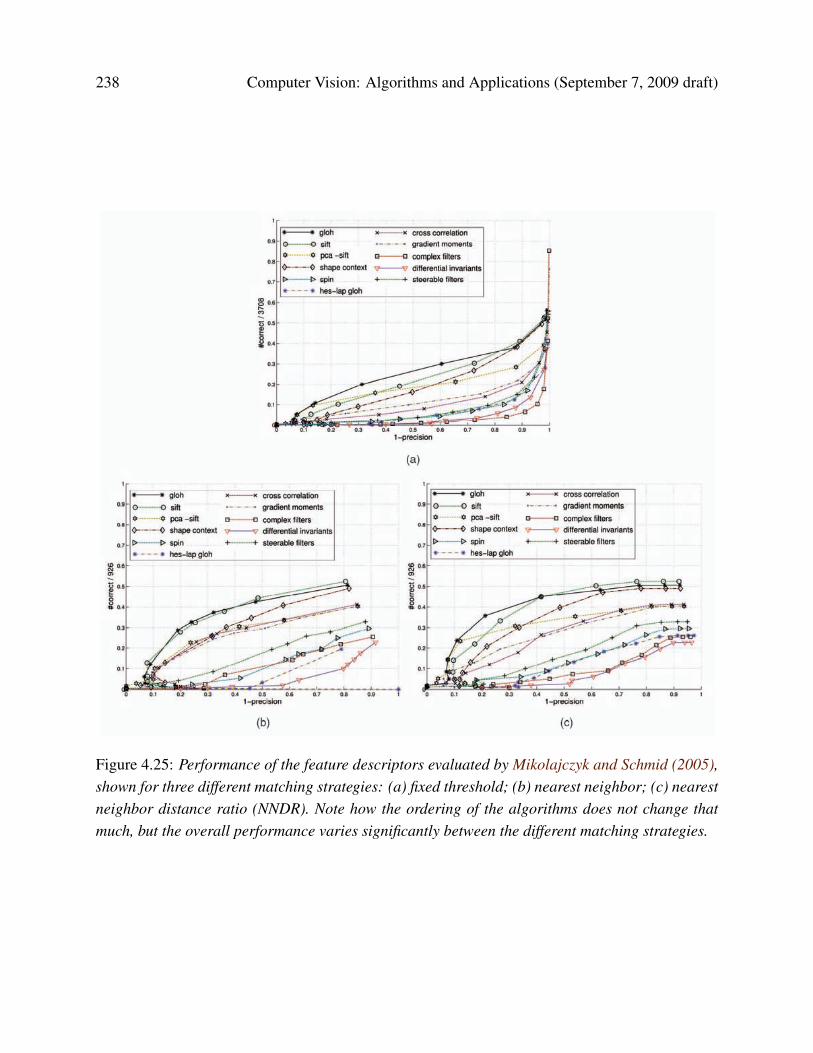
ated by Mikolajczyk and Schmid (2005) can be seen in Figure 4.25. As you can see, the nearestneighbor and NNDR strategies produce improved ROC curves.
Efficient matching
Once we have decided on a matching strategy, we still need to efficiently search for potential can-didates. The simplest way to find all corresponding feature points is to compare all features againstall other features in each pair of potentially matching images. Unfortunately, this is quadratic inthe number of extracted features, which makes it impractical for most applications.
A better approach is to devise an indexing structure such as a multi-dimensional search tree ora hash table to rapidly search for features near a given feature. Such indexing structures can eitherbe built for each image independently (which is useful if we want to only consider certain potentialmatches, e.g., searching for a particular object), or globally for all the images in a given database,which can potentially be faster, since it removes the need to iterate over each image. For extremelylarge databases (millions of images or more), even more efficient structures based on ideas fromdocument retrieval (e.g., vocabulary trees, (Nister and Stewenius 2006)) can be used §14.3.2.
One of the simpler techniques to implement is multi-dimensional hashing, which maps descrip-tors into fixed size buckets based on some function applied to each descriptor vector. At matchingtime, each new feature is hashed into a bucket, and a search of nearby buckets is used to returnpotential candidates (which can then be sorted or graded to determine which are valid matches).
A simple example of hashing is the Haar wavelets used by Brown et al. (2005) in their MOPS
238 Computer Vision: Algorithms and Applications (September 7, 2009 draft)
4.1.1 Matching Strategies
The definition of a match depends on the matching strategy.We compare three of them. In the case of threshold-basedmatching, two regions are matched if the distance betweentheir descriptors is below a threshold. A descriptor can haveseveral matches and severalof them maybecorrect. In thecaseof nearest neighbor-based matching, two regionsA andB arematched if the descriptorDB is thenearest neighbor toDA andif the distance between them is below a threshold. With thisapproach, a descriptor has only one match. The thirdmatching strategy is similar to nearest neighbor matching,except that the thresholding is applied to the distance ratiobetween the first and the second nearest neighbor. Thus, theregions are matched if jjDA �DBjj=jjDA �DCjj < t, whereDB is the first andDC is the second nearest neighbor toDA. Allmatching strategies compare each descriptor of the referenceimage with each descriptor of the transformed image.
Figs. 4a, 4b, and 4c show the results for the three matchingstrategies. The descriptors are computed on Hessian-Affineregions. The ranking of the descriptors is similar for allmatching strategies. There are some small changes betweennearest neighbor matching (NN) and matching based on thenearest neighbor distance ratio (NNDR). In Fig. 4c, which
shows the results for NNDR, SIFT is significantly better thanPCA-SIFT, whereas GLOH obtains a score similar to SIFT.Cross correlation and complex filters obtain slightly betterscores than for threshold based and nearest neighbormatching. Moments perform as well as cross correlationand PCA-SIFT in the NNDR matching (cf., Fig. 4c).
The precision is higher for the nearest neighbor-basedmatching (cf., Figs. 4b and 4c) than for the threshold-basedapproach (cf., Fig. 4a). This is because the nearest neighboris mostly correct, although the distance between similardescriptors varies significantly due to image transforma-tions. Nearest neighbor matching selects only the bestmatch below the threshold and rejects all others; therefore,there are less false matches and the precision is high.Matching based on nearest neighbor distance ratio is similarbut additionally penalizes the descriptors which have manysimilar matches, i.e., the distance to the nearest neighbor iscomparable to the distances to other descriptors. Thisfurther improves the precision. The nearest neighbor-basedtechniques can be used in the context of matching; however,they are difficult to apply when descriptors are searched ina large database. The distance between descriptors is thenthe main similarity criterion. The results for distance
1622 IEEE TRANSACTIONS ON PATTERN ANALYSIS AND MACHINE INTELLIGENCE, VOL. 27, NO. 10, OCTOBER 2005
Fig. 4. Comparison of different matching strategies. Descriptors computed on Hessian-Affine regions for images from Fig. 3e. (a) Threshold-based
matching. (b) Nearest neighbor matching. (c) Nearest neighbor distance ratio matching. hes-lap gloh is the GLOH descriptor computed for
Hessian-Laplace regions (cf., Section 4.1.4).
Figure 4.25: Performance of the feature descriptors evaluated by Mikolajczyk and Schmid (2005),shown for three different matching strategies: (a) fixed threshold; (b) nearest neighbor; (c) nearestneighbor distance ratio (NNDR). Note how the ordering of the algorithms does not change thatmuch, but the overall performance varies significantly between the different matching strategies.

4.1. Points 239
Figure 4.26: The three Haar wavelet coefficients used for hashing the MOPS descriptor devisedby Brown et al. (2005) are computed by summing each 8 × 8 normalized patch over the light anddark gray regions and taking their difference.
paper. During the matching structure construction, each 8 × 8 scaled, oriented, and normalizedMOPS patch is converted into a 3-element index by performing sums over different quadrantsof the patch (Figure 4.26). The resulting three values are normalized by their expected standarddeviations and then mapped to the two (of b = 10) nearest 1-D bins. The three-dimensional indicesformed by concatenating the three quantized values are used to index the 23 = 8 bins where thefeature is stored (added). At query time, only the primary (closest) indices are used, so only asingle three-dimensional bin needs to be examined. The coefficients in the bin can then used toselect k approximate nearest neighbors for further processing (such as computing the NNDR).
A more complex, but more widely applicable, version of hashing is called locality-sensitivehashing, which uses unions of independently computed hashing functions to index the features(Gionis et al. 1999, Shakhnarovich et al. 2006). Shakhnarovich et al. (2003) extend this techniqueto be more sensitive to the distribution of points in parameter space, which they call parameter-sensitive hashing. [ Note: Even more recent work converts high-dimensional descriptor vectorsinto binary codes that can be compared using Hamming distances (Torralba et al. 2008, Weiss etal. 2008), or better LSH (Kulis and Grauman 2009). There’s even the most recent NIPS submissionby Lana... ] [ Note: Probably won’t mention earlier work by Salakhutdinov and Hinton, since it’swell described and compared in (Weiss et al. 2008). ]
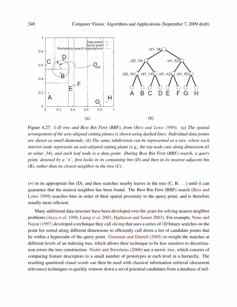
Another widely used class of indexing structures are multi-dimensional search trees. The bestknown of these are called k-D trees, which divide the multi-dimensional feature space along alter-nating axis-aligned hyperplanes, choosing the threshold along each axis so as to maximize somecriterion such as the search tree balance (Samet 1989). Figure 4.27 shows an example of a two-dimensional k-d tree. Here, eight different data points A–H are shown as small diamonds arrangedon a two-dimensional plane. The k-d tree recursively splits this plane along axis-aligned (hori-zontal or vertical) cutting planes. Each split can be denoted using the dimension number and splitvalue (Figure 4.27b). The splits are arranged so as to try to balance the tree (keep its maximumdepths as small as possible). At query time, a classic k-d tree search first locates the query point
240 Computer Vision: Algorithms and Applications (September 7, 2009 draft)
(a) (b)
Figure 4.27: k-D tree and Best Bin First (BBF), from (Beis and Lowe 1999). (a) The spatialarrangement of the axis-aligned cutting planes is shown using dashed lines. Individual data pointsare shown as small diamonds. (b) The same subdivision can be represented as a tree, where eachinterior node represents an axis-aligned cutting plane (e.g., the top node cuts along dimension d1at value .34), and each leaf node is a data point. During Best Bin First (BBF) search, a querypoint, denoted by a ’+’, first looks in its containing bin (D) and then in its nearest adjacent bin(B), rather than its closest neighbor in the tree (C).
(+) in its appropriate bin (D), and then searches nearby leaves in the tree (C, B, . . .) until it canguarantee that the nearest neighbor has been found. The Best Bin First (BBF) search (Beis andLowe 1999) searches bins in order of their spatial proximity to the query point, and is thereforeusually more efficient.
Many additional data structure have been developed over the years for solving nearest neighborproblems (Arya et al. 1998, Liang et al. 2001, Hjaltason and Samet 2003). For example, Nene andNayar (1997) developed a technique they call slicing that uses a series of 1D binary searches on thepoint list sorted along different dimensions to efficiently cull down a list of candidate points thatlie within a hypercube of the query point. Grauman and Darrell (2005) re-weight the matches atdifferent levels of an indexing tree, which allows their technique to be less sensitive to discretiza-tion errors the tree construction. Nister and Stewenius (2006) use a metric tree, which consists ofcomparing feature descriptors to a small number of prototypes at each level in a hierarchy. Theresulting quantized visual words can then be used with classical information retrieval (documentrelevance) techniques to quickly winnow down a set of potential candidates from a database of mil-
4.1. Points 241
lions of images §14.3.2. Muja and Lowe (2009) compare a number of these approaches, introducea new one of their own (priority search on hierarchical k-means trees), and conclude that multiplerandomized k-d trees often provide the best performance. Despite all of this promising work, therapid computation of image feature correspondences remains a challenging open research problem.
Feature match verification and densification
Once we have some hypothetical (putative) matches, we can often use geometric alignment §6.1 toverify which matches are inliers and which ones are outliers. For example, if we expect the wholeimage to be translated or rotated in the matching view, we can fit a global geometric transformand keep only those feature matches that are sufficiently close to this estimated transformation.The process of selecting a small set of seed matches and then verifying a larger set is often calledrandom sampling or RANSAC §6.1.4. Once an initial set of correspondences has been established,some systems look for additional matches, e.g., by looking for additional correspondences alongepipolar lines §11.1 or in the vicinity of estimated locations based on the global transform. Thesetopics will be discussed further in Sections §6.1, §11.2, and §14.3.1.
4.1.4 Feature tracking
An alternative to independently finding features in all candidate images and then matching them isto find a set of likely feature locations in a first image and to then search for their correspondinglocations in subsequent images. This kind of detect then track approach is more widely used forvideo tracking applications, where the expected amount of motion and appearance deformationbetween adjacent frames is expected to be small (or at least bounded).
The process of selecting good features to track is closely related to selecting good featuresfor more general recognition applications. In practice, regions containing high gradients in bothdirections, i.e., which have high eigenvalues in the auto-correlation matrix (4.8), provide stablelocations at which to find correspondences (Shi and Tomasi 1994).
In subsequent frames, searching for locations where the corresponding patch has low squareddifference (4.1) often works well enough. However, if the images are undergoing brightnesschange, explicitly compensating for such variations (8.9) or using normalized cross-correlation(8.11) may be preferable. If the search range is large, it is also often more efficient to use a hi-erarchical search strategy, which uses matches in lower-resolution images to provide better initialguesses and hence speed up the search §8.1.1. Alternatives to this strategy involve learning whatthe appearance of the patch being tracked should be, and then searching for it in a vicinity of itspredicted position (Avidan 2001, Jurie and Dhome 2002, Williams et al. 2003). These topics areall covered in more detail in the section on incremental motion estimation §8.1.3.

242 Computer Vision: Algorithms and Applications (September 7, 2009 draft)
Figure 4.28: Feature tracking using an affine motion model (Shi and Tomasi 1994). Top row:image patch around the tracked feature location. Bottom row: image patch after warping backtoward the first frame using an affine deformation. Even though the speed sign gets larger fromframe to frame, the affine transformation maintains a good resemblance between the original andsubsequent tracked frames.
If features are being tracked over longer image sequences, their appearance can undergo largerchanges. You then have to decide whether to continue matching against the originally detectedpatch (feature), or to re-sample each subsequent frame at the matching location. The former strat-egy is prone to failure as the original patch can undergo appearance changes such as foreshortening.The latter runs the risk of the feature drifting from its original location to some other location in theimage (Shi and Tomasi 1994). (Mathematically, one can argue that small mis-registration errorscompound to create a Markov Random Walk, which leads to larger drift over time.)
A preferable solution is to compare the original patch to later image locations using an affinemotion model §8.2. Shi and Tomasi (1994) first compare patches using a translational modelbetween neighboring frames, and then use the location estimate produced by this step to initializean affine registration between the patch in the current frame and the base frame where a feature wasfirst detected (Figure 4.28). In their system, features are only detected infrequently, i.e., only inregions where tracking has failed. In the usual case, an area around the current predicted locationof the feature is searched with an incremental registration algorithm §8.1.3.
Since their original work on feature tracking, Shi and Tomasi’s approach has generated a stringof interesting follow-on papers and applications. Beardsley et al. (1996) use extended featuretracking combined with structure from motion §7 to incrementally build up sparse 3D models fromvideo sequences. Kang et al. (1997) tie together the corners of adjacent (regularly gridded) patchesto provide some additional stability to the tracking (at the cost of poorer handling of occlusions).Tommasini et al. (1998) provide a better spurious match rejection criterion for the basic Shi andTomasi algorithm, Collins and Liu (2003) provide improved mechanisms for feature selectionand dealing with larger appearance changes over time, and Shafique and Shah (2005) develop

4.1. Points 243
Figure 4.29: Real-time head tracking using the fast trained classifiers of Lepetit et al. (2004).
algorithms for feature matching (data association) for videos with large numbers of moving objectsor points. Yilmaz et al. (2006) and Lepetit and Fua (2005) survey the larger field object tracking,which includes not only feature-based techniques but also alternative techniques such as contourand region-based techniques §5.1.
One of the newest developments in feature tracking is the use of learning algorithms to buildspecial-purpose recognizers to rapidly search for matching features anywhere in an image (Lepetitet al. 2005, Hinterstoisser et al. 2008, Rogez et al. 2008).2 By taking the time to train classifierson sample patches and their affine deformations, extremely fast and reliable feature detectors canbe constructed, which enables much faster motions to be supported. (Figure 4.29). Coupling suchfeatures to deformable models (Pilet et al. 2008) or structure-from-motion algorithms (Klein andMurray 2008) can result in even higher stability
[ Note: The Lepetit and Fua (2005) survey has lots of great info and references on tracking,and also a great Mathematical Tools section. Re-read and see if I want to incorporate more, e.g.,line-based 3D tracking. ]
2 See also my previous comment on earlier work in learning-based tracking (Avidan 2001, Jurie and Dhome 2002,Williams et al. 2003).
244 Computer Vision: Algorithms and Applications (September 7, 2009 draft)
(a) (b) (c) (d)
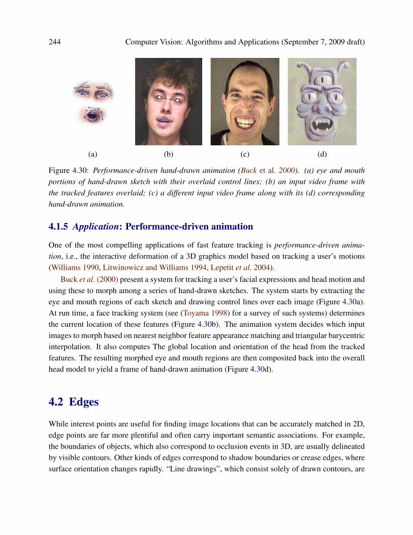
Figure 4.30: Performance-driven hand-drawn animation (Buck et al. 2000). (a) eye and mouthportions of hand-drawn sketch with their overlaid control lines; (b) an input video frame withthe tracked features overlaid; (c) a different input video frame along with its (d) correspondinghand-drawn animation.
4.1.5 Application: Performance-driven animation
One of the most compelling applications of fast feature tracking is performance-driven anima-tion, i.e., the interactive deformation of a 3D graphics model based on tracking a user’s motions(Williams 1990, Litwinowicz and Williams 1994, Lepetit et al. 2004).
Buck et al. (2000) present a system for tracking a user’s facial expressions and head motion andusing these to morph among a series of hand-drawn sketches. The system starts by extracting theeye and mouth regions of each sketch and drawing control lines over each image (Figure 4.30a).At run time, a face tracking system (see (Toyama 1998) for a survey of such systems) determinesthe current location of these features (Figure 4.30b). The animation system decides which inputimages to morph based on nearest neighbor feature appearance matching and triangular barycentricinterpolation. It also computes The global location and orientation of the head from the trackedfeatures. The resulting morphed eye and mouth regions are then composited back into the overallhead model to yield a frame of hand-drawn animation (Figure 4.30d).
4.2 Edges
While interest points are useful for finding image locations that can be accurately matched in 2D,edge points are far more plentiful and often carry important semantic associations. For example,the boundaries of objects, which also correspond to occlusion events in 3D, are usually delineatedby visible contours. Other kinds of edges correspond to shadow boundaries or crease edges, wheresurface orientation changes rapidly. “Line drawings”, which consist solely of drawn contours, are
4.2. Edges 245
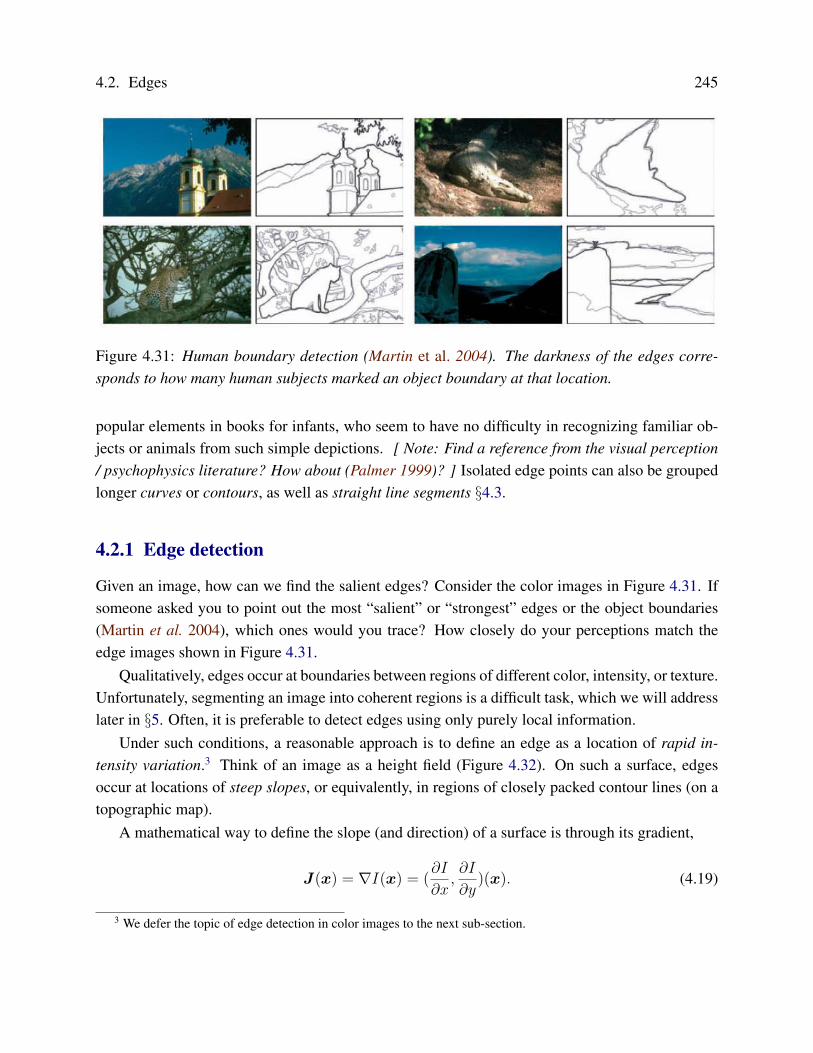
Figure 4.31: Human boundary detection (Martin et al. 2004). The darkness of the edges corre-sponds to how many human subjects marked an object boundary at that location.
popular elements in books for infants, who seem to have no difficulty in recognizing familiar ob-jects or animals from such simple depictions. [ Note: Find a reference from the visual perception/ psychophysics literature? How about (Palmer 1999)? ] Isolated edge points can also be groupedlonger curves or contours, as well as straight line segments §4.3.
4.2.1 Edge detection
Given an image, how can we find the salient edges? Consider the color images in Figure 4.31. Ifsomeone asked you to point out the most “salient” or “strongest” edges or the object boundaries(Martin et al. 2004), which ones would you trace? How closely do your perceptions match theedge images shown in Figure 4.31.
Qualitatively, edges occur at boundaries between regions of different color, intensity, or texture.Unfortunately, segmenting an image into coherent regions is a difficult task, which we will addresslater in §5. Often, it is preferable to detect edges using only purely local information.
Under such conditions, a reasonable approach is to define an edge as a location of rapid in-tensity variation.3 Think of an image as a height field (Figure 4.32). On such a surface, edgesoccur at locations of steep slopes, or equivalently, in regions of closely packed contour lines (on atopographic map).
A mathematical way to define the slope (and direction) of a surface is through its gradient,
J(x) = ∇I(x) = (∂I
∂x,∂I
∂y)(x). (4.19)
3 We defer the topic of edge detection in color images to the next sub-section.

246 Computer Vision: Algorithms and Applications (September 7, 2009 draft)
Figure 4.32: Edge detection as slope finding in a height field. The local gradient vector points inthe direction of greatest ascent and is perpendicular to the edge/contour orientation.
The local gradient vector J points in the direction of steepest ascent in the intensity function. Itsmagnitude is an indication of the slope or strength of the variation, while its orientation points in adirection perpendicular to the local contour (Figure 4.32).
Unfortunately, taking image derivatives accentuates high frequencies and hence amplifies noise(since the proportion of noise to signal is larger at high frequencies). It is therefore necessary tosmooth the image with a low-pass filter prior to computing the gradient. Because we would like theresponse of our edge detector to be independent of orientation, a circularly symmetric smoothingfilter is desirable. As we saw in §3.2.1, the Gaussian is the only separable circularly-symmetricfilter, and so it is used in most edge detection algorithms. Canny (1986) discusses alternativefilters, and (Nalwa and Binford 1986, Nalwa 1987, Deriche 1987, Freeman and Adelson 1991,Nalwa 1993, Heath et al. 1998, Crane 1997, Ritter and Wilson 2000, Bowyer et al. 2001) reviewalternative edge detection algorithms and compare their performance.
Because differentiation is a linear operation, it commutes with other linear filtering operations.The gradient of the smoothed image can therefore be written as
Jσ(x) = ∇[Gσ(x) ∗ I(x)] == [∇Gσ](x) ∗ I(x), (4.20)
i.e., we can convolve the image with the horizontal and vertical derivatives of the Gaussian kernel
4.2. Edges 247
function,
∇Gσ(x) = (∂Gσ
∂x,∂Gσ
∂y)(x) = [−x − y]
1
σ3exp
(−x
2 + y2
2σ2
)(4.21)
(The parameter σ indicates the width of the Gaussian.) This is the same computation that is per-formed by Freeman and Adelson’s (1991) first order steerable filter, which we already covered in§3.2.1 (3.27–3.28).
Figure 4.33b–c shows the result of convolving an image with the gradient of two differentGaussians. The direction of the gradient is encoded as the hue, and its strength is encoded as thesaturation/value. As you can see, the gradients are stronger is areas corresponding to what wewould perceive as edges.
For many applications, however, we wish to thin such a continuous image to only return iso-lated edges, i.e., as single pixels or edgels at discrete locations along the edge contours. This canbe achieved by looking for maxima in the edge strength (gradient magnitude) in a direction per-pendicular to the edge orientation, i.e., along the gradient direction. [ Note: It may be moreconvenient to just define the edge orientation as being the same as that of the (signed) gradient,i.e., pointing from dark to light. See Figure 2.2 for an illustration of the normal vector n used torepresent a line, and the local line equation becomes (x−xi) · ni = 0. This will make subsequentHough transform explanation simpler. ]
Finding this maximum corresponds to taking a directional derivative of the strength field in thedirection of the gradient and then looking for zero crossings. The desired directional derivative isequivalent to the dot product between a second gradient operator and the results of the first,
Sσ(x) = ∇ · Jσ(x) = [∇2Gσ](x) ∗ I(x)]. (4.22)
The gradient operator dot produced with the gradient is called the Laplacian. The convolutionkernel
∇2Gσ(x) =1
σ3
(2− x2 + y2
2σ2
)exp
(−x
2 + y2
2σ2
)(4.23)
is therefore called the Laplacian of Gaussian (LoG) kernel (Marr and Hildreth 1980). This kernelcan be split into two separable parts,
∇2Gσ(x) =1
σ3
(1− x2
2σ2
)Gσ(x)Gσ(y) +
1
σ3
(1− y2
2σ2
)Gσ(y)Gσ(x) (4.24)
(J. S. Wiejak and Buxton 1985).In practice, it is quite common to replace the Laplacian of Gaussian convolution with a Dif-
ference of Gaussian (DoG) computation, since the kernel shapes are qualitatively similar (Fig-ure 3.37). This is especially convenient if a “Laplacian pyramid” §3.4 has already been computed.4
4 Recall that Burt and Adelson’s (1983a) “Laplacian pyramid” actually computed differences of Gaussian-filteredlevels.
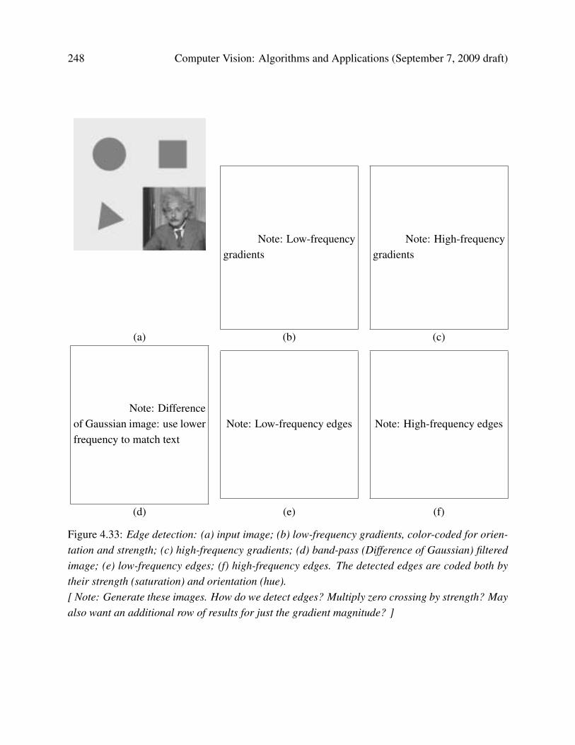
248 Computer Vision: Algorithms and Applications (September 7, 2009 draft)
Note: Low-frequencygradients
Note: High-frequencygradients
(a) (b) (c)
Note: Differenceof Gaussian image: use lowerfrequency to match text
Note: Low-frequency edges Note: High-frequency edges
(d) (e) (f)
Figure 4.33: Edge detection: (a) input image; (b) low-frequency gradients, color-coded for orien-tation and strength; (c) high-frequency gradients; (d) band-pass (Difference of Gaussian) filteredimage; (e) low-frequency edges; (f) high-frequency edges. The detected edges are coded both bytheir strength (saturation) and orientation (hue).[ Note: Generate these images. How do we detect edges? Multiply zero crossing by strength? Mayalso want an additional row of results for just the gradient magnitude? ]
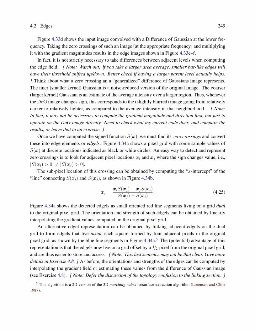
4.2. Edges 249
Figure 4.33d shows the input image convolved with a Difference of Gaussian at the lower fre-quency. Taking the zero crossings of such an image (at the appropriate frequency) and multiplyingit with the gradient magnitudes results in the edge images shown in Figure 4.33e–f.
In fact, it is not strictly necessary to take differences between adjacent levels when computingthe edge field. [ Note: Watch out: if you take a larger area average, smaller bar-like edges willhave their threshold shifted up/down. Better check if having a larger parent level actually helps.] Think about what a zero crossing an a “generalized” difference of Gaussians image represents.The finer (smaller kernel) Gaussian is a noise-reduced version of the original image. The coarser(larger kernel) Gaussian is an estimate of the average intensity over a larger region. Thus, wheneverthe DoG image changes sign, this corresponds to the (slightly blurred) image going from relativelydarker to relatively lighter, as compared to the average intensity in that neighborhood. [ Note:In fact, it may not be necessary to compute the gradient magnitude and direction first, but just tooperate on the DoG image directly. Need to check what my current code does, and compare theresults, or leave that to an exercise. ]
Once we have computed the signed function S(x), we must find its zero crossings and convertthese into edge elements or edgels. Figure 4.34a shows a pixel grid with some sample values ofS(x) at discrete locations indicated as black or white circles. An easy way to detect and representzero crossings is to look for adjacent pixel locations xi and xj where the sign changes value, i.e.,[S(xi) > 0] 6= [S(xj) > 0].
The sub-pixel location of this crossing can be obtained by computing the “x-intercept” of the“line” connecting S(xi) and S(xj), as shown in Figure 4.34b,
xz =xiS(xj)− xjS(xi)
S(xj)− S(xi). (4.25)
Figure 4.34a shows the detected edgels as small oriented red line segments living on a grid dualto the original pixel grid. The orientation and strength of such edgels can be obtained by linearlyinterpolating the gradient values computed on the original pixel grid.
An alternative edgel representation can be obtained by linking adjacent edgels on the dualgrid to form edgels that live inside each square formed by four adjacent pixels in the originalpixel grid, as shown by the blue line segments in Figure 4.34a.5 The (potential) advantage of thisrepresentation is that the edgels now live on a grid offset by a 1/2-pixel from the original pixel grid,and are thus easier to store and access. [ Note: This last sentence may not be that clear. Give moredetails in Exercise 4.8. ] As before, the orientations and strengths of the edges can be computed byinterpolating the gradient field or estimating these values from the difference of Gaussian image(see Exercise 4.8). [ Note: Defer the discussion of the topology confusion to the linking section. ]
5 This algorithm is a 2D version of the 3D marching cubes isosurface extraction algorithm (Lorensen and Cline1987).
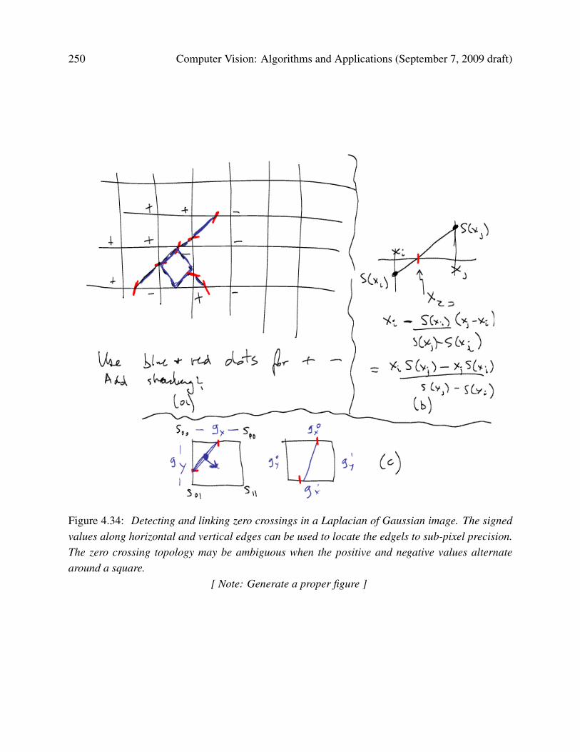
250 Computer Vision: Algorithms and Applications (September 7, 2009 draft)
Figure 4.34: Detecting and linking zero crossings in a Laplacian of Gaussian image. The signedvalues along horizontal and vertical edges can be used to locate the edgels to sub-pixel precision.The zero crossing topology may be ambiguous when the positive and negative values alternatearound a square.
[ Note: Generate a proper figure ]
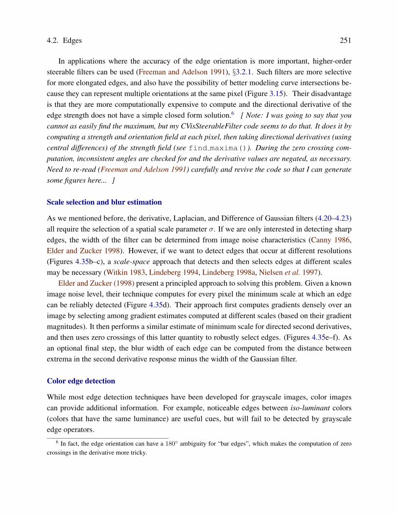
4.2. Edges 251
In applications where the accuracy of the edge orientation is more important, higher-ordersteerable filters can be used (Freeman and Adelson 1991), §3.2.1. Such filters are more selectivefor more elongated edges, and also have the possibility of better modeling curve intersections be-cause they can represent multiple orientations at the same pixel (Figure 3.15). Their disadvantageis that they are more computationally expensive to compute and the directional derivative of theedge strength does not have a simple closed form solution.6 [ Note: I was going to say that youcannot as easily find the maximum, but my CVisSteerableFilter code seems to do that. It does it bycomputing a strength and orientation field at each pixel, then taking directional derivatives (usingcentral differences) of the strength field (see find maxima()). During the zero crossing com-putation, inconsistent angles are checked for and the derivative values are negated, as necessary.Need to re-read (Freeman and Adelson 1991) carefully and revive the code so that I can generatesome figures here... ]
Scale selection and blur estimation
As we mentioned before, the derivative, Laplacian, and Difference of Gaussian filters (4.20–4.23)all require the selection of a spatial scale parameter σ. If we are only interested in detecting sharpedges, the width of the filter can be determined from image noise characteristics (Canny 1986,Elder and Zucker 1998). However, if we want to detect edges that occur at different resolutions(Figures 4.35b–c), a scale-space approach that detects and then selects edges at different scalesmay be necessary (Witkin 1983, Lindeberg 1994, Lindeberg 1998a, Nielsen et al. 1997).
Elder and Zucker (1998) present a principled approach to solving this problem. Given a knownimage noise level, their technique computes for every pixel the minimum scale at which an edgecan be reliably detected (Figure 4.35d). Their approach first computes gradients densely over animage by selecting among gradient estimates computed at different scales (based on their gradientmagnitudes). It then performs a similar estimate of minimum scale for directed second derivatives,and then uses zero crossings of this latter quantity to robustly select edges. (Figures 4.35e–f). Asan optional final step, the blur width of each edge can be computed from the distance betweenextrema in the second derivative response minus the width of the Gaussian filter.
Color edge detection
While most edge detection techniques have been developed for grayscale images, color imagescan provide additional information. For example, noticeable edges between iso-luminant colors(colors that have the same luminance) are useful cues, but will fail to be detected by grayscaleedge operators.
6 In fact, the edge orientation can have a 180◦ ambiguity for “bar edges”, which makes the computation of zerocrossings in the derivative more tricky.

252 Computer Vision: Algorithms and Applications (September 7, 2009 draft)
(a) (b) (c)
(d) (e) (f)
Figure 4.35: Scale selection for edge detection (Elder and Zucker 1998). (a) original image; (b–c) Canny/Deriche edge detector tuned to the finer (mannequin) and coarser (shadow) scales; (d)minimum reliable scale for gradient estimation; (e) minimum reliable scale for second derivativeestimation; (f) final detected edges.
One simple approach is to combine the outputs of grayscale detectors run on each color bandseparately.7 However, some care must be taken. For example, if we simply sum up the gradientsin each of the color bands, the signed gradients may actually cancel each other! (Consider, forexample a pure red-to-green edge.) We could also detect edges independently in each band andthen take the union of these, but this might lead to thickened or doubled edges that are hard to link.
A better approach is to compute the oriented energy in each band (Morrone and Burr 1988,Perona and Malik 1990a), e.g., using a second order steerable filter §3.2.1 (Freeman and Adelson1991), and to then sum up the orientation-weighted energies and find their joint best orientation.
7 Instead of using the raw RGB space, a more perceptually uniform color space such as L*a*b* §2.3.2 can be usedinstead. When trying to match human performance (Martin et al. 2004), this makes sense. However, in terms of thephysics of the underlying image formation and sensing, this may be questionable.

4.2. Edges 253
Unfortunately, the directional derivative of this energy may not have a closed form solution (as inthe case of signed first order steerable filters), so a simple zero crossing-based strategy cannot beused. However, the technique described by Elder and Zucker (1998) can be used to numericallycompute these zero crossings instead.
An alternative approach is to estimate local color statistics in regions around each pixel (Ruzonand Tomasi 2001, Martin et al. 2004). This has the advantage that more sophisticated techniquescan be used to compare regional statistics (e.g., 3D color histograms) and that additional measures,such as texture, can also be considered. Figure 4.36 shows the output of such detectors.
Of course, many other approaches have been developed for detecting color edges, dating backto early work by Nevatia (1977). Ruzon and Tomasi (2001) and Gevers et al. (2006) provide goodreviews of these approaches, which include ideas such as fusing outputs from multiple channels,using multidimensional gradients, and vector-based methods.
Combining edge feature cues
If the goal of edge detection is to match human boundary detection performance (Bowyer et al.2001, Martin et al. 2004), as opposed to simply finding stable features for matching, even betterdetectors can be constructed by combining multiple low-level cues such as brightness, color, andtexture.
Martin et al. (2004) describe a system that combines brightness, color, and texture edges toproduce state-of-the-art performance on a database of hand-segmented natural color images (Mar-tin et al. 2001). First, they construct and train separate oriented half-disc detectors for measuringsignificant differences in brightness (luminance), color (a* and b* channels, summed responses),and texture (un-normalized filter bank responses from (Malik et al. 2001)). (The training uses 200labeled image, and testing is performed on a different set of 100 images.) Next, some of theseresponses are sharpened using a soft non-maximal suppression technique. Finally, the outputs ofthe three detectors are combined using a variety of machine learning techniques, among which, lo-gistic regression is found to have the best speed-space-accuracy tradeoff. The resulting system (seeFigure 4.36 for some visual examples) is shown to outperform previously developed techniques. Inmore recent work, Maire et al. (2008) improve on these results by combining the local appearancebased detector with a spectral (segmentation-based) detector (Belongie and Malik 1998). [ Note:Even more recently, Arbelaez et al. (2009) build a hierarchical segmentation on top of this edgedetector using a variant of the watershed algorithm. ]
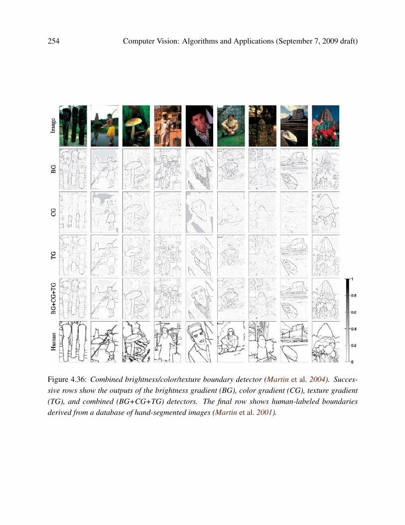
254 Computer Vision: Algorithms and Applications (September 7, 2009 draft)
Figure 4.36: Combined brightness/color/texture boundary detector (Martin et al. 2004). Succes-sive rows show the outputs of the brightness gradient (BG), color gradient (CG), texture gradient(TG), and combined (BG+CG+TG) detectors. The final row shows human-labeled boundariesderived from a database of hand-segmented images (Martin et al. 2001).

4.2. Edges 255
Figure 4.37: Chain code representation of a grid-aligned linked edge chain. The code is repre-sented as a series of direction codes, e.g, 0 1 0 7 6 5, which can further be compressed.
4.2.2 Edge linking
While isolated edges can be useful for a variety of applications such as line detection §4.3 andsparse stereo matching §11.2, they become even more useful when linked into continuous contours.
If the edges have been detected using zero crossings of some function, linking them up isstraightforward, since adjacent edgels share common endpoints (Figure 4.34a). Linking the edgelsinto chains involves picking up an unlinked edgel and following its neighbors in both directions.Either a sorted list of edgels (sorted first say by x coordinates and then y coordinates) or a 2D arraycan be used to accelerate the neighbor finding. If edges were not detected using zero crossings,finding the continuation of an edgel can be tricky. In this case, comparing the orientation (andoptionally phase) of adjacent edgels can be used for disambiguation. Ideas from connected com-ponent computation can also sometimes be used to make the edge linking process even faster (seeExercise 4.9).
Once the edgels have been linked into chains, we can apply an optional thresholding withhysteresis to remove low-strength contour segments (Canny 1986). [ Note: Do I need to say morehere? If so, re-read Canny and describe this better. ]
Linked edgel lists can be encoded more compactly using a variety of alternative representa-tions. A chain code encodes a list of connected points lying on an N8 grid using a different 3-bitcode corresponding to the eight cardinal directions (N, NE, E, SE, S, SW, W, NW) between apoint and its successor (Figure 4.37). While this representation is more compact than the originaledgel list (especially if predictive variable-length coding is used), it is not very suitable for furtherprocessing.

256 Computer Vision: Algorithms and Applications (September 7, 2009 draft)
Figure 4.38: Arc-length parameterization of a contour. Discrete points along the contour are firsttranscribed as (x, y) pairs along the arc length s. This curve can then be regularly re-sampled orconverted into alternative (e.g., Fourier) representations.
Figure 4.39: Matching two contours using their arc-length parameterization. If both curves arenormalized to unit length, s ∈ [0, 1], they will have the same descriptor up to an overall “temporal”shift (due to different starting points for s = 0) and a phase (x-y) shift due to rotation.
A more useful representation is the arc-length parameterization of a contour, x(s), where sdenotes the arc length along a curve. Consider the linked set of edgels shown in Figure 4.38a.We start at one point (the solid dot at (1.0, 0.5) in Figure 4.38a) and plot it at coordinate s = 0
(Figure 4.38b). The next point at (2.0, 0.5) gets plotted at s = 1, and the next point at (2.5, 1.0)
gets plotted at s = 1.7071, i.e., we increment s by the length of each edge segment. The resultingplot can be resampled on a regular (say integral) s grid before further processing.
The advantage of the arc-length parameterization is that it makes matching and processing (e.g.,smoothing) operations much easier. Consider the two curves describing similar shapes shownin Figure 4.39. To compare the curves, we first subtract the average values x0 =
∫s x(s) from
each descriptor. Next, we rescale each descriptor so that s goes from 0 to 1 instead of 0 to S,i.e., we divide x(s) by S. Finally, we take the Fourier transform of each normalized descriptor,

4.2. Edges 257
Figure 4.40: Curve smoothing with a Gaussian kernel (Lowe 1988): (a) without shrinkage correc-tion term; (b) with shrinkage correction term.
treating each x = (x, y) value as a complex number. If the original curves are the same (up to anunknown scale and rotation), the resulting Fourier transforms should differ only by a scale changein magnitude plus a constant phase shift, due to rotation, and a linear phase shift, due to differentstarting points for s (see Exercise 4.10). [ Note: See if you can find a reference to this Fouriermatching, either in a textbook or in some papers. ]
[ Note: Read the papers below before finishing off this section: ]Lowe (1989): as we filter a 2D curve with a Gaussian, estimate the second derivatives of the
smoothed curves (x and y separately), and then add back a term to compensate for the shrinkage(which is a function of radius and hence second derivative). See Figure 4.40. Taubin (1995)extends this technique by replacing the Lowe’s offsetting step with one based on an additional(larger) smoothing...
An alternative approach, based on selectively modifying different frequencies in a wavelet de-composition, is presented by Finkelstein and Salesin (1994). In addition to controlling shrinkagewithout affecting its “sweep”, wavelets allow the “character” of a curve to be interactively modi-fied, as shown in Figure 4.41.
Kimia’s curve evolution and skeleton-based descriptors: nice review article (Tek and Kimia2003) and applications to recognition (Sebastian and Kimia 2005).
Also, shape contexts (Belongie et al. 2002).Latest global contour grouping, completion, and junction detection (Maire et al. 2008): run
normalized cuts (NC) on affinities derived from strongest Pb edge, then take gradients of eigen-vectors to get “global Pb” and then later Pj (probability of junction) [ Note: Even more recently,

258 Computer Vision: Algorithms and Applications (September 7, 2009 draft)
Figure 4.41: Changing the character of a curve without affecting its sweep (Finkelstein and Salesin1994): higher frequency wavelets can be replaced with exemplars from a style library to effectdifferent local appearances.
Arbelaez et al. (2009) build a hierarchical segmentation on top of this edge detector using a variantof the watershed algorithm. ]
Point to (Maire et al. 2008) for other recent edge detectors and contour linkers.Meltzer and Soatto (2008) have a nice edge descriptor based on scale-space analysis followed
by gradient histograms on each side of the edge. Can be used for wide baseline stereo.
4.2.3 Application: Edge editing and enhancement
While edges can serve as components for object recognition or features for matching, they can alsobe used directly for image editing.
In fact, if the edge magnitude and blur estimate are kept along with each edge, a visually similarimage can be reconstructed from this information (Elder 1999). Based on this principle, Elderand Golderg (2001) propose a system for “Image Editing in the Contour Domain”. Their systemallows users to selectively remove edges corresponding to unwanted features such as specularities,shadows, or distracting visual elements. After reconstructing the image from the remaining edges,the undesirable visual features have been removed (Figure 4.42).
Another potential application is to enhance perceptually salient edges while simplifying theunderlying image to produce a cartoon-like or “pen-and-ink” like stylized image (DeCarlo andSantella 2002). This application is discussed in more detail in the section on non-photorealisticrendering §10.5.2.

4.3. Lines 259
(a) (b) (c)
(d) (e) (f)
Figure 4.42: Image editing in the contour domain (Elder and Golderg 2001). (a) & (d): originalimages; (b) & (e): extracted edges (edges to be deleted are marked in white); (c) & (f): recon-structed edited images.
4.3 Lines
While edges and general curves are suitable for describing the contours of natural objects, theman-made worlds is full of straight lines. Detecting and matching these lines can be useful in avariety of applications, including architectural modeling, pose estimation in urban environments,and the analysis of printed document layouts.
[ Note: Add a figure that shows each of the 3 cases (successive approx., Hough, VP) below? ]
In this section, we present some techniques for extracting piecewise linear descriptions fromthe curves computed in the previous section. We begin with some algorithms for approximating acurve as a piecewise-linear polyline. We then describe the Hough transform, which can be usedto group edgels into line segments even across gaps and occlusions. Finally, we describe how 3Dlines with common vanishing points can be grouped together. These vanishing points can be usedto calibrate a camera and to determine its orientation relative to a rectahedral scene, as describedin §6.3.2.

260 Computer Vision: Algorithms and Applications (September 7, 2009 draft)
(a) (b) (c)
Figure 4.43: Approximating a curve (shown in black) as a polyline or B-spline: (a) original curveand a polyline approximation shown in red; (b) successive approximation by recursively findingpoints furthest away from the current approximation (Ramer 1972, Douglas and Peucker 1973);(c) B-spline approximation, with the control net shown in blue and the B-spline shown in red.[ Note: Visio does this when you draw a free-form curve: if you hover over the (smoothed) curve,you can see the Bezier control points. ]
4.3.1 Successive approximation
As we saw in the previous section 4.2.2, describing a curve as a series of 2D locations xi =
x(si) provides a general representation suitable for matching and further processing. In manyapplications, however, it is preferable to approximate such a curve with a simpler representation,e.g., as a piecewise-linear polyline or as a B-spline curve (Farin 1996), as shown in Figure 4.43.
Many techniques have been developed over the years to perform this approximation, whichis also known as line simplification. One of the oldest, and simplest, is the one simultaneouslyproposed by Ramer (1972) and Douglas and Peucker (1973), who recursively subdivide the curveat the point(s) the furthest away from the line(s) joining the two endpoints (or the current coarsepolyline approximation), as shown in Figure 4.43. Hershberger and Snoeyink (1992) provide amore efficient implementation and also cite some of the other related work in this area.
Once the line simplification has been computed, it can be used to approximate the originalcurve. If a smoother representation or visualization is desired, either approximating or interpolat-ing splines or curves can be used §3.4.1 and §5.1.1 (Szeliski and Ito 1986, Bartels et al. 1987, Farin1996), as shown in Figure 4.43c.
4.3.2 Hough transforms
While curve approximation with polylines can often lead to successful line extraction, lines in thereal world are sometimes broken up into disconnected components or made up of many collinearline segments (Figure 4.44). In many cases, it is desirable to group such collinear line segmentsinto extended lines. As a further processing stage, described in the next section §4.3.3, we can then

4.3. Lines 261
Figure 4.44: Line fitting to discontinuous edge segments: (a) image with clutter; (b) fitted lines;(c) checkerboard image with missing edgels at corners.
(a) (b)
Figure 4.45: Original Hough transform: (a) each point votes for a complete family of potentiallines ri(θ) = xi cos θ + yi sin θ; (b) each pencil of lines sweeps out a sinusoid in (r, θ); theirintersection provides the desired line equation.

262 Computer Vision: Algorithms and Applications (September 7, 2009 draft)
(a) (b)
Figure 4.46: Hough transform: (a) an edgel re-parameterized in polar (r, θ) coordinates, withni = (cos θi, sin θi) and r=ni · xi; (b) (r, θ) accumulator array, showing the votes for the threeedgels marked in red, green, and blue.
y
xdθ
nl
^
Figure 4.47: 2D line equation expressed in terms of the normal n and distance to the origin d(coped from Figure 2.2).
group such lines into collections with common vanishing points.The Hough transform, named after its original inventor (Hough 1962), is a well-known tech-
nique for having edges “vote” for plausible line locations (Duda and Hart 1972, Ballard 1981,Illingworth and Kittler 1988) [ Note: Add more references: (Forsyth and Ponce 2003, Fit-ting Chapter); (Jahne 1997); ] In its original formulation (Figure 4.45), each edge point votesfor all possible lines passing through it, and lines corresponding to high accumulator or bin val-ues are examined for potential line fits.8 Unless the points on a line are truly punctate, a betterapproach (in my experience) is to use the local orientation information at each edgel to vote fora single accumulator cell (Figure 4.46), as described below. A hybrid strategy, where each edgel
8 The Hough transform can also be generalized to look for other geometric features such as circles (Ballard 1981),but we do not cover such extensions in this book.

4.3. Lines 263
votes for a number of possible orientation/location pairs centered around the estimate orientation,may be desirable in some cases.
Before we can vote for line hypotheses, we must first choose a suitable representation. Fig-ure 4.47 (copied from Figure 2.2) shows the normal-distance (n, d) parameterization for a line.Since lines are made up of edge segments, we adopt the convention that the line normal n pointsin the same direction (has the same signs) as the image gradient J(x) = ∇I(x) (4.19). To obtaina minimal two-parameter representation for lines, we convert the normal vector into an angle
θ = tan−1 ny/nx, (4.26)
as shown in Figure 4.47. The range of possible (θ, d) values is [−180◦, 180◦]× [−√
2,√
2], assum-ing that we are using normalized pixel coordinates (2.61) that lie in [−1, 1]. The number of binsto use along each axis depends on the accuracy of the position and orientation estimate availableat each edgel and the expected line density, and is best set experimentally with some test runs onsample imagery.
Given the line parameterization, the Hough transform proceeds as follows: [ Note: turn intoan algorithm ]
1. Clear the accumulator array.
2. For each detected edgel at location (x, y) and orientation θ = tan−1 ny/nx, compute thevalue of
d = xnx + y ny (4.27)
and increment the accumulator corresponding to (θ, d).
3. Find the peaks in the accumulator corresponding to lines.
4. Optionally re-fit the lines to the constituent edgels.
Note that the original formulation of the Hough transform, which assumed no knowledge of theedgel orientation θ, has an additional loop inside of step 2 that iterates over all possible values of θand increments a whole series of accumulators.
There are a lot of details in getting the Hough transform to work well, but these are best workedout by writing an implementation and testing it out on sample data. Exercise 4.14 describes some ofthese steps in more detail, including using edge segment lengths and/or strength during the votingprocess, keeping a list of constituent edgels in the accumulator array for easier post-processing,and optionally combining edges of different “polarity” into the same line segments.
An alternative to the 2D polar representation (θ, d) representation for lines is to use the full 3Dm = (n, d) line equation, projected onto the unit sphere. While the sphere can be parameterized
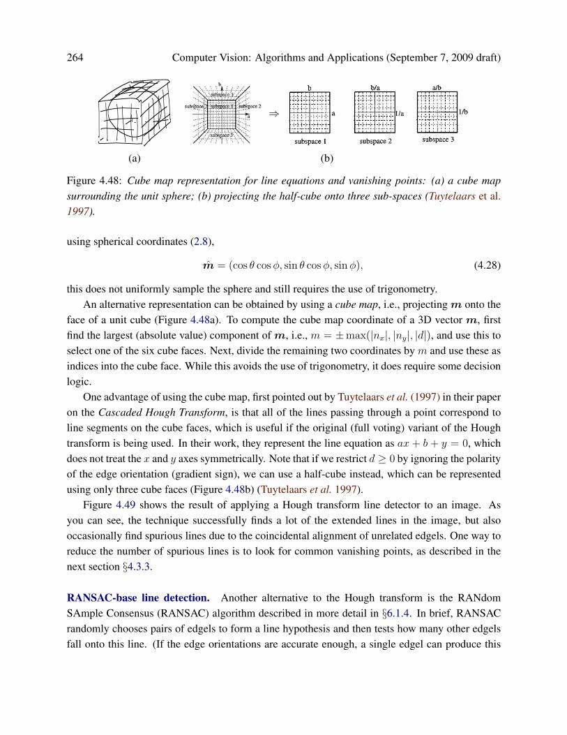
264 Computer Vision: Algorithms and Applications (September 7, 2009 draft)
⇒
(a) (b)
Figure 4.48: Cube map representation for line equations and vanishing points: (a) a cube mapsurrounding the unit sphere; (b) projecting the half-cube onto three sub-spaces (Tuytelaars et al.1997).
using spherical coordinates (2.8),
m = (cos θ cosφ, sin θ cosφ, sinφ), (4.28)
this does not uniformly sample the sphere and still requires the use of trigonometry.An alternative representation can be obtained by using a cube map, i.e., projecting m onto the
face of a unit cube (Figure 4.48a). To compute the cube map coordinate of a 3D vector m, firstfind the largest (absolute value) component of m, i.e., m = ±max(|nx|, |ny|, |d|), and use this toselect one of the six cube faces. Next, divide the remaining two coordinates by m and use these asindices into the cube face. While this avoids the use of trigonometry, it does require some decisionlogic.
One advantage of using the cube map, first pointed out by Tuytelaars et al. (1997) in their paperon the Cascaded Hough Transform, is that all of the lines passing through a point correspond toline segments on the cube faces, which is useful if the original (full voting) variant of the Houghtransform is being used. In their work, they represent the line equation as ax + b + y = 0, whichdoes not treat the x and y axes symmetrically. Note that if we restrict d ≥ 0 by ignoring the polarityof the edge orientation (gradient sign), we can use a half-cube instead, which can be representedusing only three cube faces (Figure 4.48b) (Tuytelaars et al. 1997).
Figure 4.49 shows the result of applying a Hough transform line detector to an image. Asyou can see, the technique successfully finds a lot of the extended lines in the image, but alsooccasionally find spurious lines due to the coincidental alignment of unrelated edgels. One way toreduce the number of spurious lines is to look for common vanishing points, as described in thenext section §4.3.3.
RANSAC-base line detection. Another alternative to the Hough transform is the RANdomSAmple Consensus (RANSAC) algorithm described in more detail in §6.1.4. In brief, RANSACrandomly chooses pairs of edgels to form a line hypothesis and then tests how many other edgelsfall onto this line. (If the edge orientations are accurate enough, a single edgel can produce this

4.3. Lines 265
Note: Some Hough-based line detection results
Figure 4.49: Some Hough-based line detection results[ Note: Show both accumulator array and overlaid lines ]
hypothesis.) Lines with sufficiently large numbers of inliers (matching edgels) are then selected asthe desired line segments.
An advantage of RANSAC is that no accumulator array is needed and so the algorithm can bemore space efficient (and potentially less prone to the choice of bin size). The disadvantage is thatmany more hypotheses may be generated and tested than those obtained by finding peaks in theaccumulator array.
In general, there is no clear consensus on which line estimation technique performs the best.It is therefore a good idea to think carefully about the problem at hand and to implement severalapproaches (successive approximation, Hough, and/or RANSAC) to determine the one that worksbest for your application.
4.3.3 Vanishing points
In many scenes, structurally important lines have the same vanishing point because they have theyare parallel. Examples of such lines are horizontal and vertical building edges, zebra crossings,railway tracks, the edges of furniture such as tables and dressers, and of course, the ubiquitouscalibration pattern (Figure 4.50). Finding the vanishing points common to such line sets can helprefine their position in the image, and, in certain cases, help determine the intrinsic and extrinsicorientation of the camera §6.3.2.
Over the years, a large number of techniques have been developed for finding vanishing points,including (Quan and Mohr 1989, Collins and Weiss 1990, Brillaut-O’Mahoney 1991, McLeanand Kotturi 1995, Becker and Bove 1995, Shufelt 1999, Tuytelaars et al. 1997, Schaffalitzky andZisserman 2000, Antone and Teller 2000, Rother 2002, Kosecka and Zhang 2005, Pflugfelder2008)–see some of the more recent papers for additional references. In this section, we present
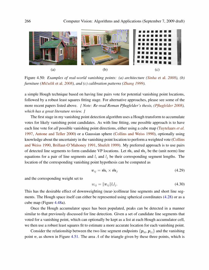
266 Computer Vision: Algorithms and Applications (September 7, 2009 draft)
(a) (b) (c)
Figure 4.50: Examples of real-world vanishing points: (a) architecture (Sinha et al. 2008), (b)furniture (Micusık et al. 2008), and (c) calibration patterns (Zhang 1999).
a simple Hough technique based on having line pairs vote for potential vanishing point locations,followed by a robust least squares fitting stage. For alternative approaches, please see some of themore recent papers listed above. [ Note: Re-read Roman Pflugfelder’s thesis, (Pflugfelder 2008),which has a great literature review. ]
The first stage in my vanishing point detection algorithm uses a Hough transform to accumulatevotes for likely vanishing point candidates. As with line fitting, one possible approach is to haveeach line vote for all possible vanishing point directions, either using a cube map (Tuytelaars et al.1997, Antone and Teller 2000) or a Gaussian sphere (Collins and Weiss 1990), optionally usingknowledge about the uncertainty in the vanishing point location to perform a weighted vote (Collinsand Weiss 1990, Brillaut-O’Mahoney 1991, Shufelt 1999). My preferred approach is to use pairsof detected line segments to form candidate VP locations. Let mi and mj be the (unit norm) lineequations for a pair of line segments and li and lj be their corresponding segment lengths. Thelocation of the corresponding vanishing point hypothesis can be computed as
vij = mi × mj (4.29)
and the corresponding weight set towij = ‖vij‖lilj. (4.30)
This has the desirable effect of downweighting (near-)collinear line segments and short line seg-ments. The Hough space itself can either be represented using spherical coordinates (4.28) or as acube map (Figure 4.48a).
Once the Hough accumulator space has been populated, peaks can be detected in a mannersimilar to that previously discussed for line detection. Given a set of candidate line segments thatvoted for a vanishing point, which can optionally be kept as a list at each Hough accumulator cell,we then use a robust least squares fit to estimate a more accurate location for each vanishing point.
Consider the relationship between the two line segment endpoints {pi0,pi1} and the vanishingpoint v, as shown in Figure 4.51. The area A of the triangle given by these three points, which is
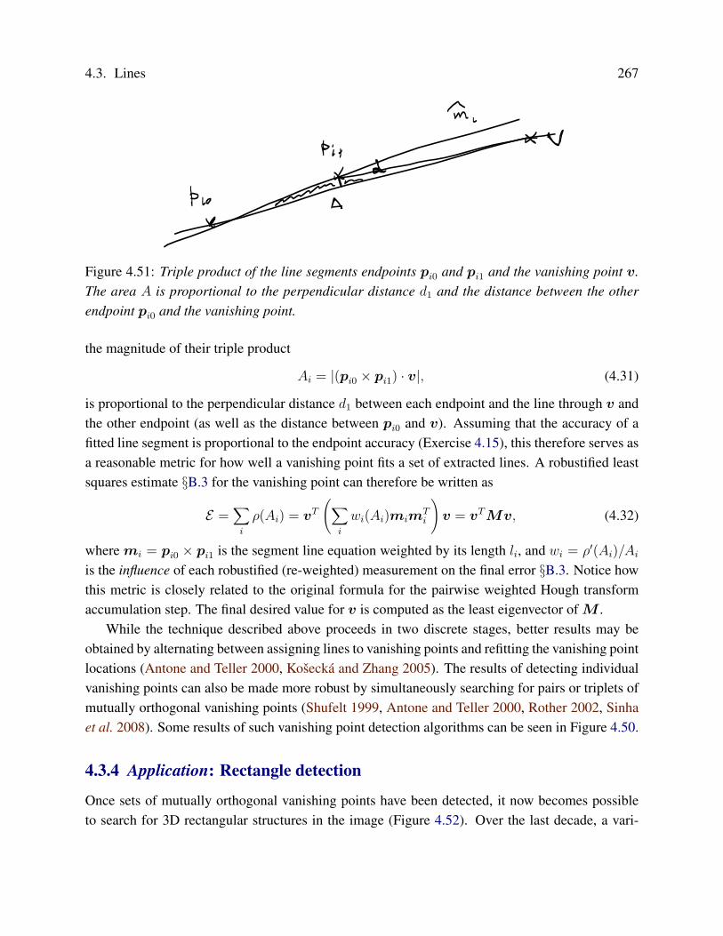
4.3. Lines 267
Figure 4.51: Triple product of the line segments endpoints pi0 and pi1 and the vanishing point v.The area A is proportional to the perpendicular distance d1 and the distance between the otherendpoint pi0 and the vanishing point.
the magnitude of their triple product
Ai = |(pi0 × pi1) · v|, (4.31)
is proportional to the perpendicular distance d1 between each endpoint and the line through v andthe other endpoint (as well as the distance between pi0 and v). Assuming that the accuracy of afitted line segment is proportional to the endpoint accuracy (Exercise 4.15), this therefore serves asa reasonable metric for how well a vanishing point fits a set of extracted lines. A robustified leastsquares estimate §B.3 for the vanishing point can therefore be written as
E =∑
i
ρ(Ai) = vT(∑
i
wi(Ai)mimTi
)v = vTMv, (4.32)
where mi = pi0 × pi1 is the segment line equation weighted by its length li, and wi = ρ′(Ai)/Aiis the influence of each robustified (re-weighted) measurement on the final error §B.3. Notice howthis metric is closely related to the original formula for the pairwise weighted Hough transformaccumulation step. The final desired value for v is computed as the least eigenvector ofM .
While the technique described above proceeds in two discrete stages, better results may beobtained by alternating between assigning lines to vanishing points and refitting the vanishing pointlocations (Antone and Teller 2000, Kosecka and Zhang 2005). The results of detecting individualvanishing points can also be made more robust by simultaneously searching for pairs or triplets ofmutually orthogonal vanishing points (Shufelt 1999, Antone and Teller 2000, Rother 2002, Sinhaet al. 2008). Some results of such vanishing point detection algorithms can be seen in Figure 4.50.
4.3.4 Application: Rectangle detection
Once sets of mutually orthogonal vanishing points have been detected, it now becomes possibleto search for 3D rectangular structures in the image (Figure 4.52). Over the last decade, a vari-

268 Computer Vision: Algorithms and Applications (September 7, 2009 draft)
(a) (b) (c)
(d) (e) (f)
Figure 4.52: Examples of rectangle detection: (a) indoor corridor and (b) building exterior withgrouped facades (Kosecka and Zhang 2005); (c) grammar-based recognition (Han and Zhu 2005);(d–e) rectangle matching using plane sweep (Micusık et al. 2008).
ety of techniques have been developed to find such rectangles, primarily focused on architecturalscenes (Kosecka and Zhang 2005, Han and Zhu 2005, Shaw and Barnes 2006, Micusık et al. 2008,Schindler et al. 2008).
After detecting orthogonal vanishing directions, Kosecka and Zhang (2005) refine the fittedline equations, search for corners near line intersections, and then verify rectangle hypotheses byrectifying the corresponding patches and looking for a preponderance of horizontal and verticaledges (Figures 4.52a–b). In follow-on work, Micusık et al. (2008) use a Markov Random Field(MRF) to disambiguate between potentially overlapping rectangle hypotheses. They also use aplane sweep algorithm to match rectangles between different views (Figures 4.52d–f).
A different approach is proposed by Han and Zhu (2005), who use a grammar of potentialrectangle shapes and nesting structures (between rectangles and vanishing points) to infer the mostlikely assignment of line segments to rectangles (Figure 4.52c).

4.4. Additional reading 269
4.4 Additional reading
[ Note: Move some references here ]An early well-regarded paper on straight line extraction in images is (Burns et al. 1986).
4.5 Exercises
Ex 4.1 (Interest point detector) Implement one or more keypoint detectors and compare theirperformance (with your own, or with a classmate’s)
Possible detectors:
1. Laplacian or Difference of Gaussian
2. Forstner-Harris Hessian (try different formula variants given in (4.9–4.11)).
3. oriented/steerable filter, either looking for 2nd order high 2nd response, or two edges in awindow (Koethe 2003), discussed in §4.1.1.
4. others from (Mikolajczyk et al. 2005, Tuytelaars and Mikolajczyk 2007)
Additional optional steps could include:
1. Compute the detections on a sub-octave pyramid and find 3D maxima.
2. Find local orientation estimates (using steerable filter responses or a gradient histogrammingmethod).
3. Implement non-maximal suppression, such as the adaptive technique of Brown et al. (2005).
4. Vary the window shape and size (pre-filter and aggregation).
To test for repeatability, download the code from http://www.robots.ox.ac.uk/˜vgg/software/
(Mikolajczyk et al. 2005, Tuytelaars and Mikolajczyk 2007), or simply rotate/shear your own testimages (pick a domain you may want to use later, e.g., for outdoor stitching).
Measure the stability of your scale and orientation estimates as well.
Ex 4.2 (Interest point descriptor) Implement one or more descriptors (steered to local scale andorientation) and compare their performance (with your own, or with a classmate’s)
Some possible descriptors include
1. contrast-normalized patches (Brown et al. 2005)
270 Computer Vision: Algorithms and Applications (September 7, 2009 draft)
2. SIFT (Lowe 2004),
3. GLOH (Mikolajczyk and Schmid 2005),
4. DAISY (Winder and Brown 2007),
5. others from (Mikolajczyk and Schmid 2005)
(Figures 4.19–4.20). Optionally do this on a sub-octave pyramid, find 3D maxima.Vary the choose window shape and size (pre-filter and aggregation);
Ex 4.3 (Feature matcher) [ Note: The following ideas are pretty old; update them: ]Use SSD or correlation score; estimate bias/gain; use local feature vector (Schmid, Jets [Von
Der Malsburg ?])How about David Lowe’s adaptive threshold idea, used in MOPS (Brown et al. 2005)?See also §8.1.2 and Exercise 8.1 for more techniques and a more quantitative comparison.
Ex 4.4 (ROC curve computation) Given a pair of curves (histograms) plotting the number ofmatching and non-matching features as a function of Euclidean distance d as shown in Figure 4.23b,derive an algorithm for plotting an ROC curve (Figure 4.23a). In particular, let t(d) be the distribu-tion of true matches and f(d) be the distribution of (false) non-matches. Write down the equationsfor the ROC, i.e., TPR(FPR), and the AUC.
Hint: Plot the cumulative distributions T (d) =∫t(d) and F (d) =
∫f(d) and see if these help
you derive the TPR and FPR at a given threshold θ.
Ex 4.5 (Image matcher—part 1) Select some set of image features (corners, lines, regions) thatyou can somewhat reliably match across images taken from disparate points of view. (Lowe 1999,Schaffalitzky and Zisserman 2002, Sivic and Zisserman 2003)
Later exercise will show how to combine this with camera motion / 3D structure to completelymatch the images.
Ex 4.6 (Feature tracker) find corresponding points, string together; (optional: winnow out matcheswith epipolar geometry or 3D – need material in next 2 chapters) add new points at each frame;evaluate quality of matches, terminate if necessary.
Note that affine registration used in (Shi and Tomasi 1994) is not introduced until §8.2 andExercise 8.2.
Ex 4.7 (Facial feature tracker) initialize tracker on person’s facial features, use it to drive a sim-ple 2D morph of another face or cartoon (reuse morphing code from exercise in previous chapter)

4.5. Exercises 271
struct SEdgel {
float e[2][2]; // edgel endpoints (zero crossing)
float x, y; // sub-pixel edge position (midpoint)
float n_x, n_y; // orientation, as normal vector
float theta; // orientation, as angle (degrees)
float length; // length of edgel
float strength; // strength of edgel (local gradient magnitude)
};
struct SLine : public SEdgel {
float line_length; // length of line (estimated from ellipsoid)
float sigma; // estimated std. dev. of edgel noise
float r; // line equation: x * n_y - y * n_x = r
};
Table 4.2: A potential C++ structure for edgel and line elements[ Note: Use a smaller font for the code. Should these kinds of code snippets be moved into AppendixC.2? ]
Ex 4.8 (Edge detector) Implement an edge detector of your choice. Compare its performance tothat of other classmates’, or from code downloaded from the Net.
A simple but well-performing sub-pixel edge detector can be created as follows:
1. Blur the input image a little,Bσ(x) = Gσ(x) ∗ I(x).
2. Construct a Gaussian pyramid (Exercise refex:pyramid),
P = Pyramid{Bσ(x)}
3. Subtract an interpolated coarser-level pyramid image from the original resolution blurredimage,
S(x) = Bσ(x)− P.InterpolatedLevel(L).
4. For each quad of pixels, {(i, j), (i+ 1, j), (i, j+ 1), (i+ 1, j+ 1)}, count the number of zerocrossings along the four edges.
5. When there are exactly two zero crossing, compute their locations using (4.25) and storethese edgel endpoints along with the midpoint in the edgel structure (Table 4.2).

272 Computer Vision: Algorithms and Applications (September 7, 2009 draft)
6. For each edgel, compute the local gradient by taking the horizontal and vertical differencesbetween the values of S along the zero crossing edges (Figure 4.34c). [ Note: Perhaps makethis a separate figure closer to the end of this chapter. ]
7. Store the magnitude of this gradient as the edge strength, and either its orientation, or that ofthe segment joining the edgel endpoints, as the edge orientation.
8. Add the edgel to a list of edgels, or alternatively, store it in a 2D array of edgels (addressedby pixel coordinates).
Table 4.2 shows a possible representation for each computed edgel.
Ex 4.9 (Edge linking and thresholding) Link up the edges computed in the previous exerciseinto chains, and optionally perform thresholding with hysteresis.
Some suggested steps include:
1. Store the edgels either in a 2D array (say an integer image with indices into the edgel list),or pre-sort the edgel list first by (integer) x coordinates and then y coordinates, for fasterneighbor finding.
2. Pick up an edgel from the the list of unlinked edgels, and find its neighbors in both directionsuntil no neighbor is found, or a closed contour is obtained. Flag edgels as linked as you visitthem, and push them onto your list of linked edgels.
3. Alternatively, generalize a previously developed connected component algorithm (Exer-cise 3.14) to perform the linking in just two raster passes.
4. [Optional] Perform hysteresis-based thresholding (Canny 1986). Starting at one end of thecontour, walk along the contour until... [ Note: Re-read Canny to see if a good descriptionexists there... ]
5. [Optional] Link together contours that have small gaps but whose endpoints have similarorientations.
6. [Optional] Find junctions between adjacent contours, e.g., using some of the ideas (or refer-ences) from (Maire et al. 2008).
Ex 4.10 (Contour matching) Convert a closed contour (linked edgel list) into its arc-length pa-rameterization, and use this to match object outlines. [ Note: See some of Kimia’s papers (Tekand Kimia 2003, Sebastian and Kimia 2005) for examples and references. ]
Some suggested steps include:

4.5. Exercises 273
1. Walk along the contour and create a list of (xi, yi, si) triplets, using the arc-length formula
si+1 = si + ‖xi+1 − xi‖. (4.33)
2. Resample this list onto a regular set of (xj, yj, j) samples using linear interpolation of eachsegment.
3. Compute the average value of x and y, e.g., x =∑j=0...S xj . (Careful: the value of S =
max si is generally non-integral, so adjust your formula accordingly.)
4. [Variant] Directly resample the original (xi, yi, si) piecewise linear function onto a length-independent set of samples, say j ∈ [0, 1023]. (Using a power of 2 length will make subse-quent Fourier transforms more convenient.)
5. Compute the Fourier transform of the curve, treating each (x, y) pair as a complex number.
6. To compare two curves, fit a linear equation to the phase difference between the two curves.(Careful: phase wraps around at 360◦. Also, you may wish to weight samples by theirFourier spectrum magnitude. See §8.1.2.)
7. [Optional] Prove that the constant phase component corresponds to the temporal shift in s,while the linear component corresponds to rotation.
Of course, feel free to try any other curve descriptor and matching technique from the computervision literature.
Ex 4.11 (Jigsaw puzzle solver–project) Write a program to automatically solve a jigsaw puzzlefrom a set of scanned puzzle pieces. The project may include the following components:
1. Scan the pieces (either face up or face down) on a flatbed scanner with a distinctively coloredbackground.
2. Optionally scan in the box top to use as a low-resolution reference image.
3. Use color-based thresholding to isolate the pieces.
4. Extract the contour of each piece using edge finding and linking.
5. Optionally re-represent each contour using an arc-length or some other re-parameterization.Break up the contours into meaningful matchable pieces (hard?).
6. Optionally associate color values with each contour to help in the matching.
274 Computer Vision: Algorithms and Applications (September 7, 2009 draft)
7. Optionally match pieces to the reference image using some rotationally invariant featuredescriptors.
8. Solve a global optimization or (backtracking) search problem to snap pieces together and/orplace them in the correct location relative to the reference image.
9. Test your algorithm on a succession of more difficult puzzles, and compare your results withothers’.
Ex 4.12 (Artistic rendering) application: ink-and-watercolor rendering (see above)...? [ Note:move this to Computational Photography chapters since we have an NPR section §10.5.2 there. ]
Ex 4.13 (Successive approximation line detector) Implement a line simplification algorithm §4.3.1(Ramer 1972, Douglas and Peucker 1973) to convert a hand-drawn curve (or linked edge image)into a small set of polylines. Optionally, re-render this curve using either an approximating orinterpolating spline or Bezier curve (Szeliski and Ito 1986, Bartels et al. 1987, Farin 1996).
Ex 4.14 (Hough transform line detector) Implement a Hough transform for finding lines in im-ages:
1. Create an accumulator array of the appropriate use-specified size and clear it. The user canspecify the spacing in degrees between orientation bins and in pixels between distance bins.The array can either be allocated as integer (for simple counts), floating point (for weightedcounts), or as an array of vectors for keeping back pointers to the constituent edges.
2. For each detected edgel at location (x, y) and orientation θ = tan−1 ny/nx, compute thevalue of
d = xnx + yny (4.34)
and increment the accumulator corresponding to (θ, d). Optionally weight the vote of eachedge by its length (see Exercise 4.8) and/or the strength of its gradient.
3. Optionally smooth the scalar accumulator array by adding in values from its immediateneighbors (this helps counteract the discretization effect of voting for only a single bin—seeExercise 3.7.
4. Find the largest peaks (local maxima) in the accumulator corresponding to lines.
5. For each peak, optionally re-fit the lines to the constituent edgels, using total least squares§A.2. In this step, optionally use the original edgel lengths and/or strength weights to weightthe least squares fit, as well as potentially the agreement between the hypothesized line

4.5. Exercises 275
orientation and the edgel orientation. Determine whether these heuristics help increase theaccuracy of the fit.
6. After fitting each peak, zero-out or eliminate that peak and its adjacent bins in the array, andmove on to the next largest peak.
Test out your Hough transform on a variety of images taken indoors and outdoors, as well ascheckerboard calibration patterns.
For the latter case (checkerboard patterns), you can modify your Hough transform by collapsingantipodal bins (θ± 180◦,−d) with (θ, d) to find lines that do not care about polarity changes. Canyou think of examples in real world images where this might be desirable as well?
Ex 4.15 (Line fitting uncertainty) Estimate the uncertainty (covariance) in your line fit using un-certainty analysis.
1. After determining which edgels belong to the line segment (using either successive approxi-mation or Hough transform), re-fit the line segment using total least square (Van Huffel andVandewalle 1991, Huffel and Lemmerling 2002), i.e., find the mean/centroid of the edgelsand then use eigenvalue analysis to find the dominant orientation.
2. Compute the perpendicular errors (deviations) to the line and robustly estimate the varianceof the fitting noise using an estimator such as MAD §B.3.
3. Optionally re-fit the line parameters by throwing away outliers or using a robust norm /influence function.
4. Estimate the error in the perpendicular location of the line segment and its orientation
[ Note: Need to work this out in more detail, and perhaps include the error analysis in the maintext. ]
Ex 4.16 (Vanishing points) Compute vanishing points and refine line equations. The results willused later to track a target (Exercise 6.5) or reconstruct architecture (Exercise ???)
Ex 4.17 (Vanishing point uncertainty) Perform an uncertainty analysis on your estimated van-ishing points. You will need to decide how to represent your vanishing point, e.g., homogeneouscoordinates on a sphere, to handle VPs near infinity.
See the discussion of Bingham distributions in (Collins and Weiss 1990).