05 - Feature Detection

• Overview• Feature Detection

– Intensity Extrema– Blob Detection– Corner Detection

• Feature Descriptors• Feature Matching• Conclusion

Overview

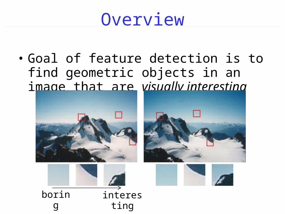
• Goal of feature detection is to find geometric objects in an image that are visually interesting

boring interesting

Overview

• Features typically have descriptors that capture local geometric properties in the image

• Features descriptors can be used for a wide range of computer vision applications:– Align multiple images to each other– Track the motion of objects in an image sequence– Perform object or face recognition – Detect defects in manufactured objects

Feature Detection

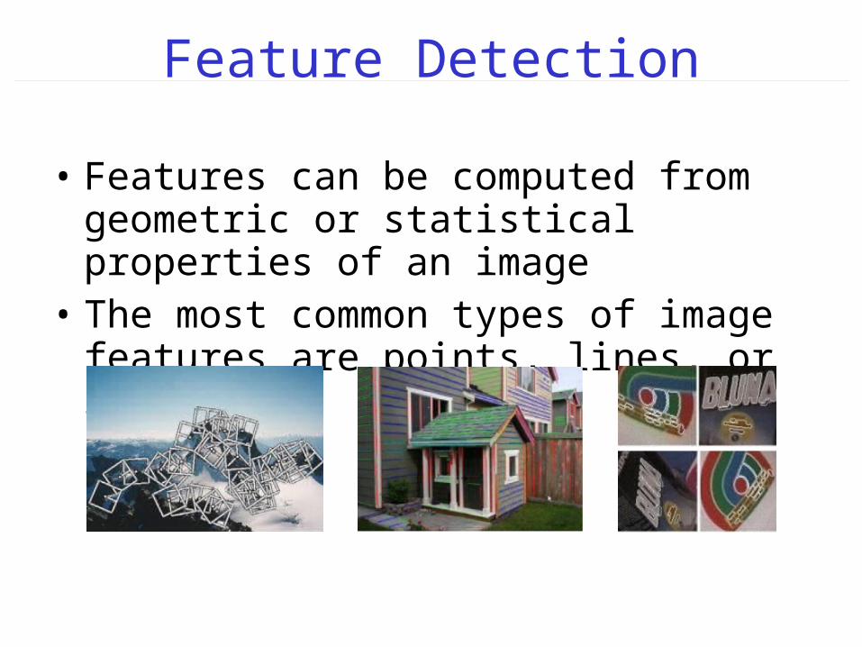
• Features can be computed from geometric or statistical properties of an image

• The most common types of image features are points, lines, or regions

Feature Detection

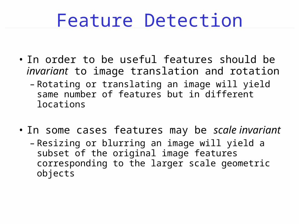
• In order to be useful features should be invariant to image translation and rotation– Rotating or translating an image will yield same

number of features but in different locations

• In some cases features may be scale invariant– Resizing or blurring an image will yield a subset of

the original image features corresponding to the larger scale geometric objects

Feature Detection

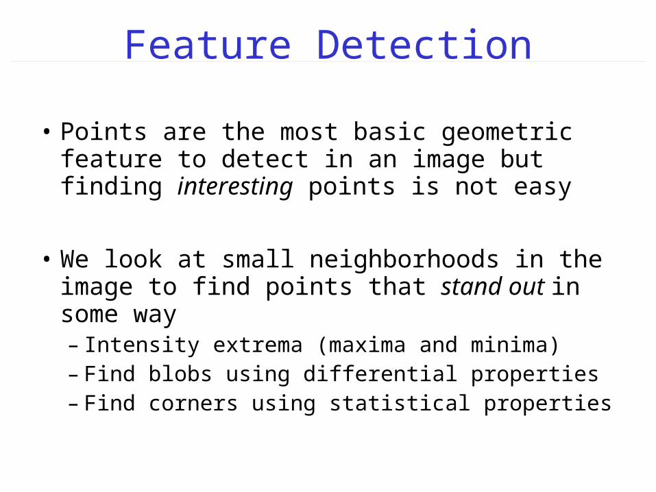
• Points are the most basic geometric feature to detect in an image but finding interesting points is not easy

• We look at small neighborhoods in the image to find points that stand out in some way– Intensity extrema (maxima and minima)– Find blobs using differential properties– Find corners using statistical properties

Intensity Extrema

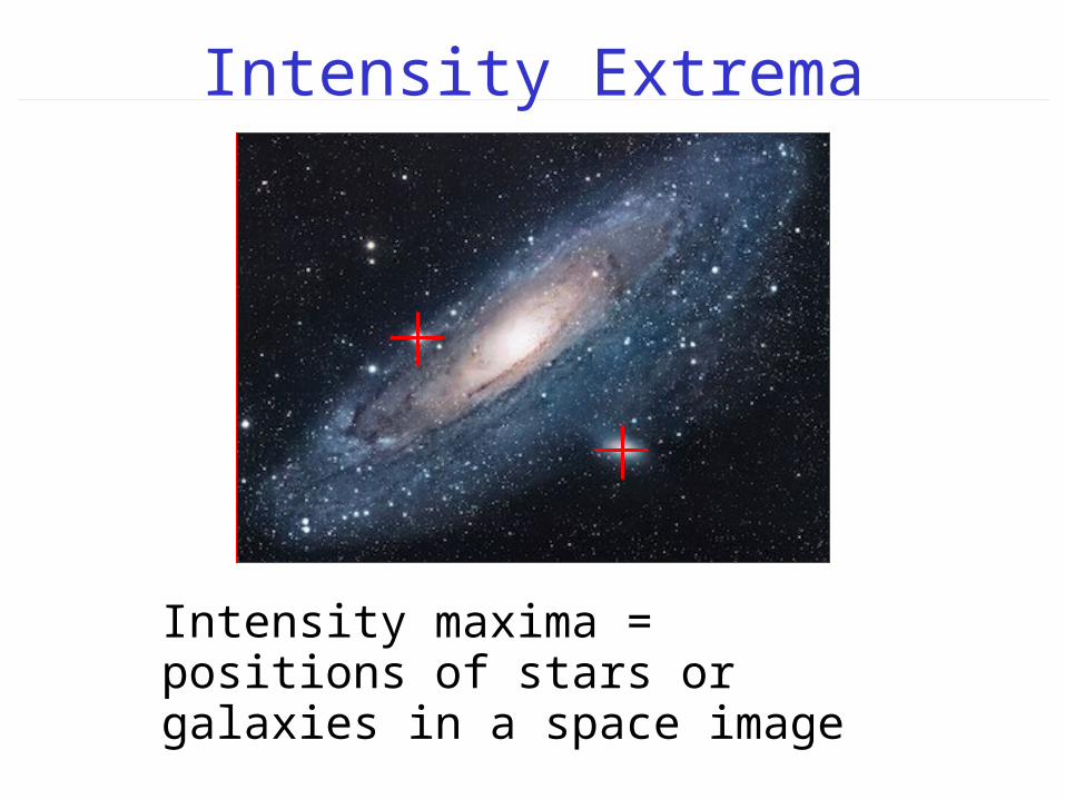
Intensity maxima = positions of stars or galaxies in a space image

Intensity Extrema

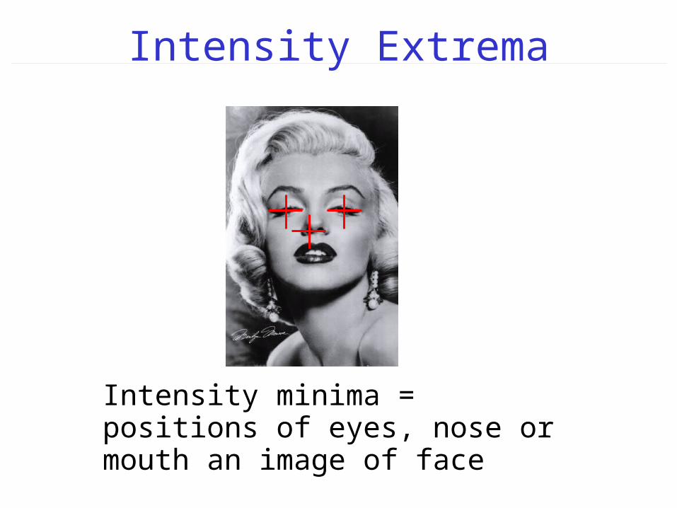
Intensity minima = positions of eyes, nose or mouth an image of face

Intensity Extrema

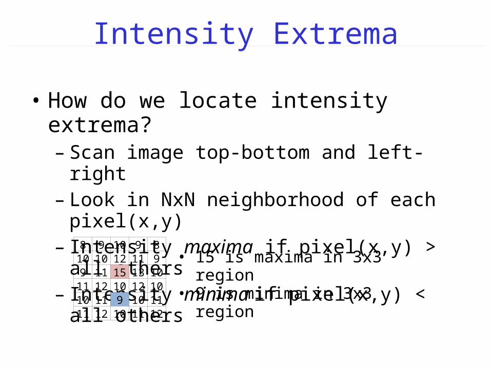
• How do we locate intensity extrema?– Scan image top-bottom and left-right– Look in NxN neighborhood of each pixel(x,y)– Intensity maxima if pixel(x,y) > all others– Intensity minima if pixel(x,y) < all others

8 9 10 9 810 10 12 11 99 11 15 13 1011 12 10 12 1010 11 9 10 1111 12 10 11 12

• 15 is maxima in 3x3 region• 9 is minima in 3x3 region

Intensity Extrema

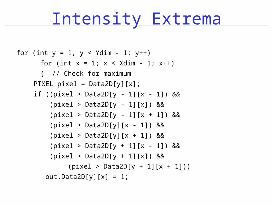
for (int y = 1; y < Ydim - 1; y++)

for (int x = 1; x < Xdim - 1; x++)

{ // Check for maximum

PIXEL pixel = Data2D[y][x];

if ((pixel > Data2D[y - 1][x - 1]) &&

(pixel > Data2D[y - 1][x]) &&

(pixel > Data2D[y - 1][x + 1]) &&

(pixel > Data2D[y][x - 1]) &&

(pixel > Data2D[y][x + 1]) &&

(pixel > Data2D[y + 1][x - 1]) &&

(pixel > Data2D[y + 1][x]) &&

(pixel > Data2D[y + 1][x + 1]))

out.Data2D[y][x] = 1;

Intensity Extrema

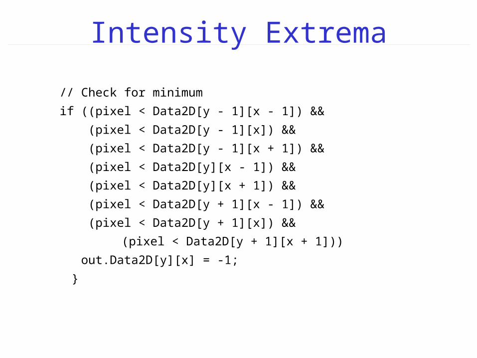
// Check for minimum

if ((pixel < Data2D[y - 1][x - 1]) &&

(pixel < Data2D[y - 1][x]) &&

(pixel < Data2D[y - 1][x + 1]) &&

(pixel < Data2D[y][x - 1]) &&

(pixel < Data2D[y][x + 1]) &&

(pixel < Data2D[y + 1][x - 1]) &&

(pixel < Data2D[y + 1][x]) &&

(pixel < Data2D[y + 1][x + 1]))

out.Data2D[y][x] = -1;

}

Intensity Extrema

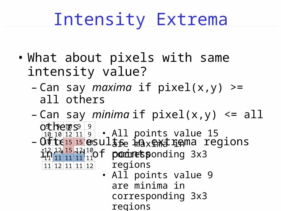
• What about pixels with same intensity value?– Can say maxima if pixel(x,y) >= all others– Can say minima if pixel(x,y) <= all others– Often results in extrema regions instead of points

9 9 10 9 910 10 12 11 910 11 15 15 1012 12 15 12 1011 11 11 11 1111 12 11 11 12

• All points value 15 are maxima in corresponding 3x3 regions

• All points value 9 are minima in corresponding 3x3 regions

Intensity Extrema

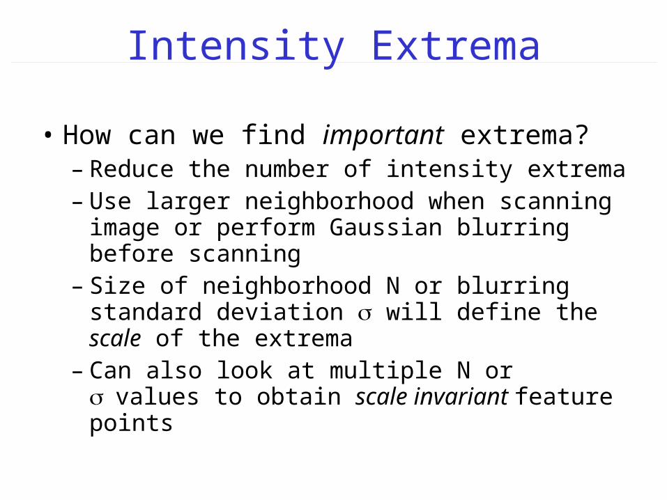
• How can we find important extrema?– Reduce the number of intensity extrema – Use larger neighborhood when scanning image or

perform Gaussian blurring before scanning– Size of neighborhood N or blurring standard

deviation will define the scale of the extrema– Can also look at multiple N or values to obtain

scale invariant feature points

Intensity Extrema

= 1

Intensity Extrema

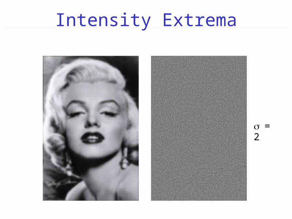
= 2

Intensity Extrema

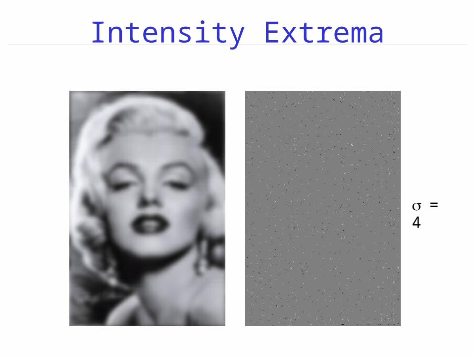
= 4

Intensity Extrema

= 8

Blob Detection

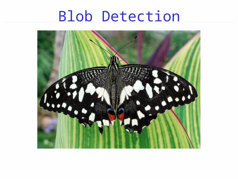
• The goal of blob detection is to locate regions of an image that are visibly lighter or darker than their surrounding regions

• One way to detect blobs is to – Look at NxN regions in an image and calculate

average intensities inside / outside radius R– Light blob: average inside >> average outside– Dark blob: average inside << average outside

Blob Detection

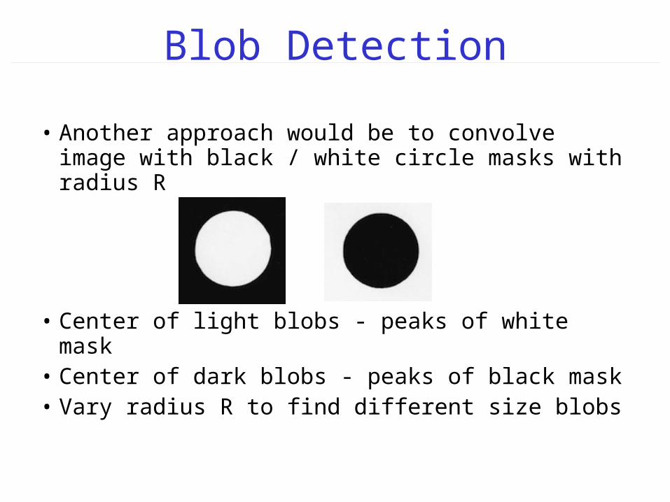
• Another approach would be to convolve image with black / white circle masks with radius R

• Center of light blobs - peaks of white mask • Center of dark blobs - peaks of black mask• Vary radius R to find different size blobs

Blob Detection

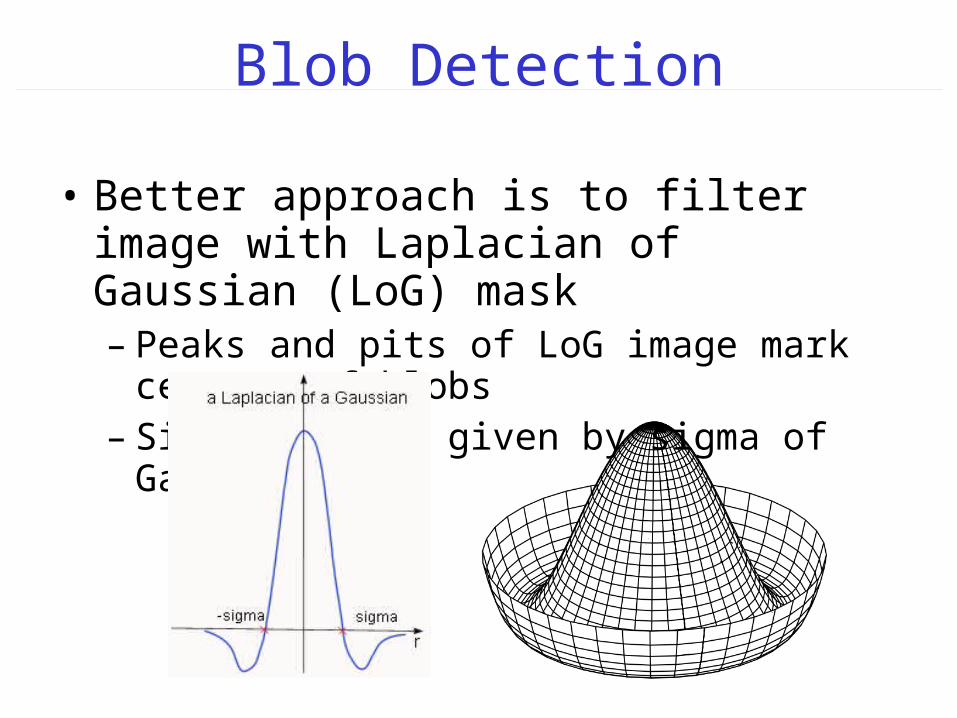
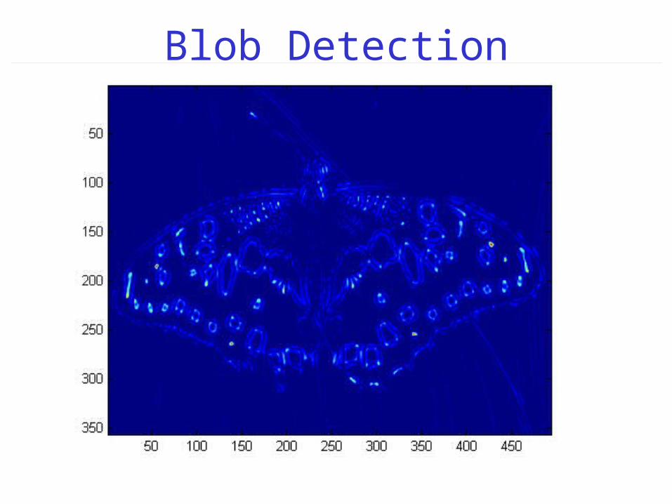
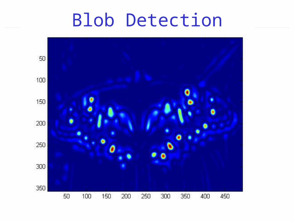
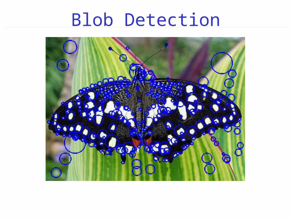
• Better approach is to filter image with Laplacian of Gaussian (LoG) mask– Peaks and pits of LoG image mark centers of blobs– Size of blobs given by sigma of Gaussian

Blob Detection

Blob Detection

Blob Detection

Blob Detection

Blob Detection

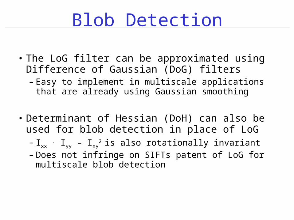
• The LoG filter can be approximated using Difference of Gaussian (DoG) filters– Easy to implement in multiscale applications that are

already using Gaussian smoothing

• Determinant of Hessian (DoH) can also be used for blob detection in place of LoG– Ixx . Iyy – Ixy

2 is also rotationally invariant– Does not infringe on SIFTs patent of LoG for

multiscale blob detection

Corner Detection

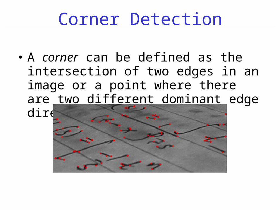
• A corner can be defined as the intersection of two edges in an image or a point where there are two different dominant edge directions

Corner Detection

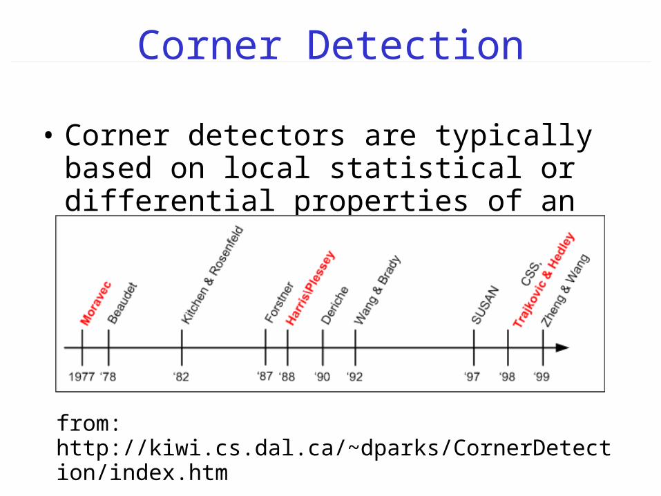
• Corner detectors are typically based on local statistical or differential properties of an image

from: http://kiwi.cs.dal.ca/~dparks/CornerDetection/index.htm

Corner Detection

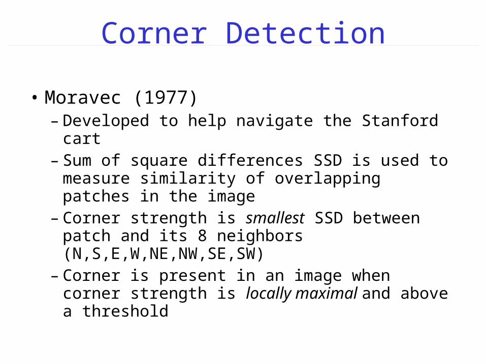
• Moravec (1977)– Developed to help navigate the Stanford cart– Sum of square differences SSD is used to measure

similarity of overlapping patches in the image– Corner strength is smallest SSD between patch and

its 8 neighbors (N,S,E,W,NE,NW,SE,SW)– Corner is present in an image when corner strength

is locally maximal and above a threshold

Corner Detection

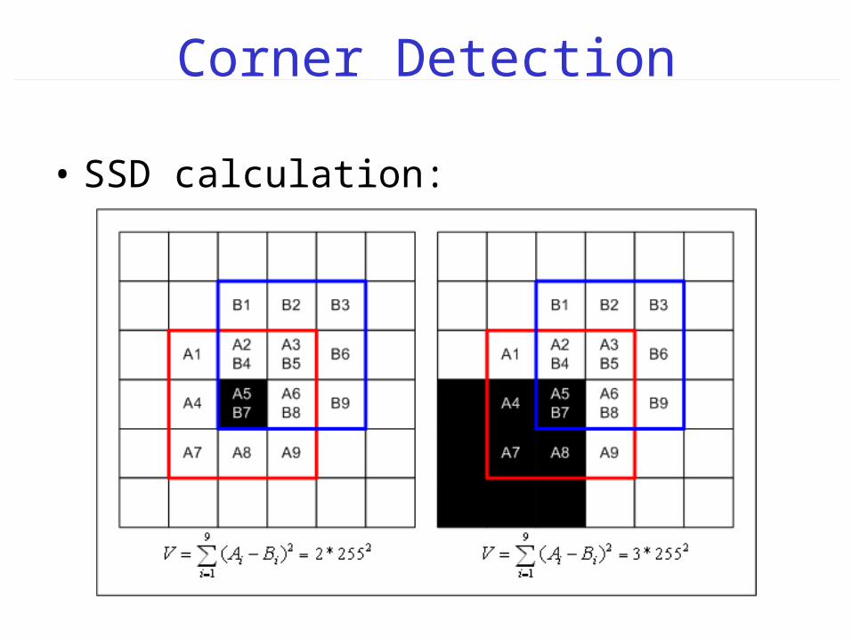
• SSD calculation:

Corner Detection

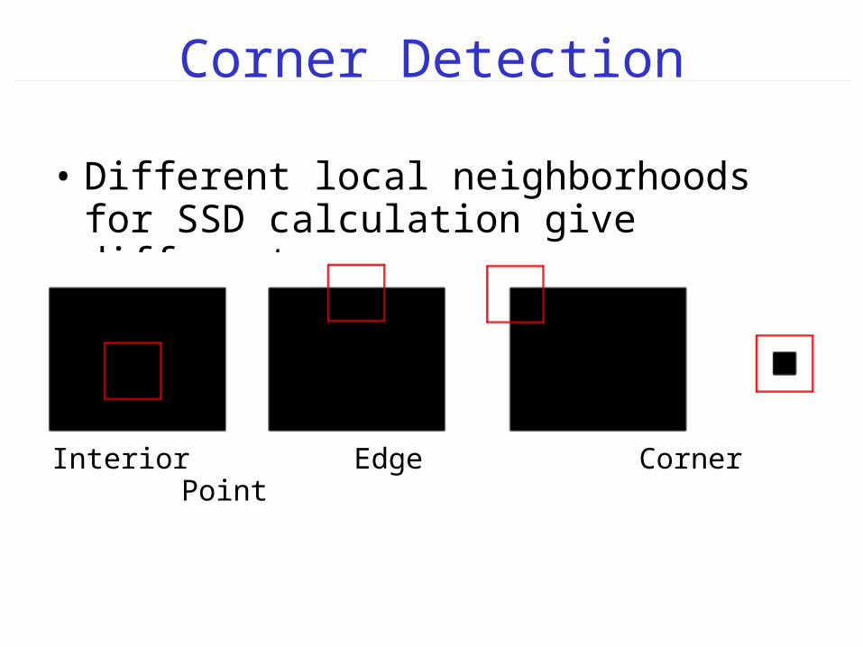
• Different local neighborhoods for SSD calculation give different corner responses

Interior Edge CornerPoint

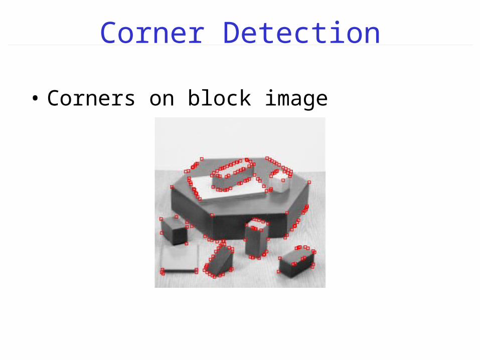
Corner Detection

• Corners on block image

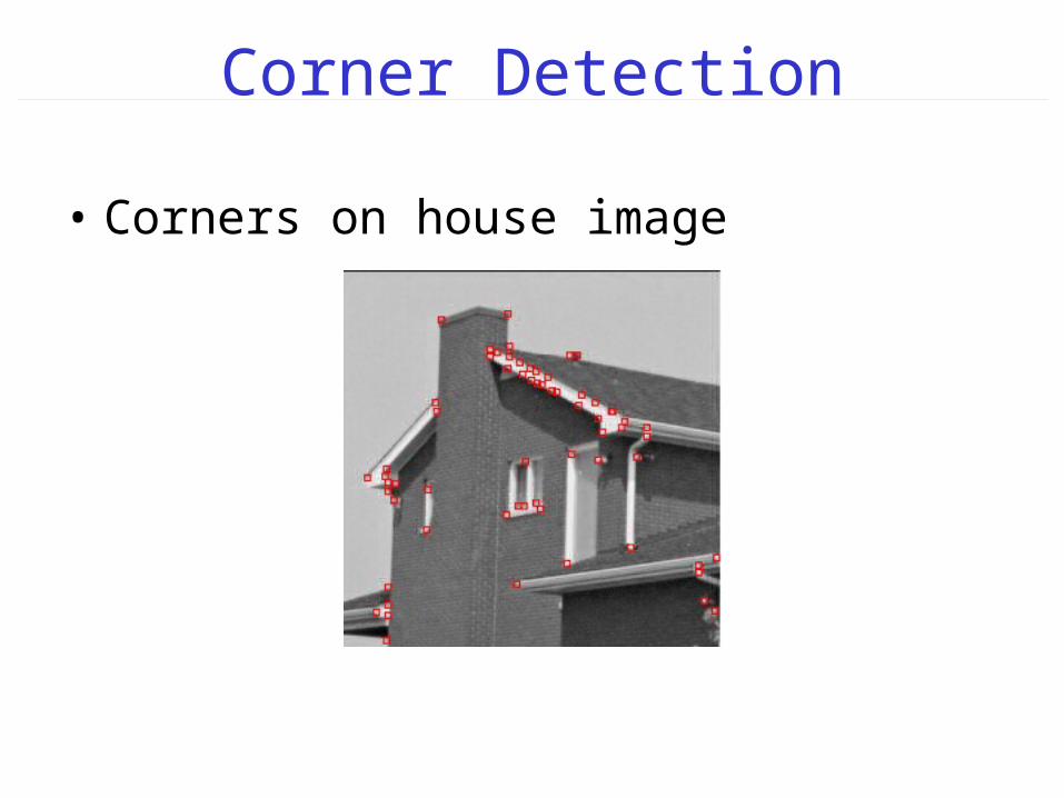
Corner Detection

• Corners on house image

Feature Descriptors

• Feature detection locates (x,y) points in an image that are interesting in some way– These (x,y) locations by themselves are not very

useful for computer vision applications

• We use feature descriptors to capture what makes these points interesting– We want local geometric properties that are

invariant to translation, rotation, and scaling

Feature Descriptors

• What local geometric information can we obtain from a point in an image?– We can look at differential properties– We can look at statistical properties

• The most common approach is to look at the image gradient near feature points

• Gradient magnitude = (Ix2 + Iy

2)1/2

• Gradient direction = arctan(Iy / Ix)

Feature Descriptors

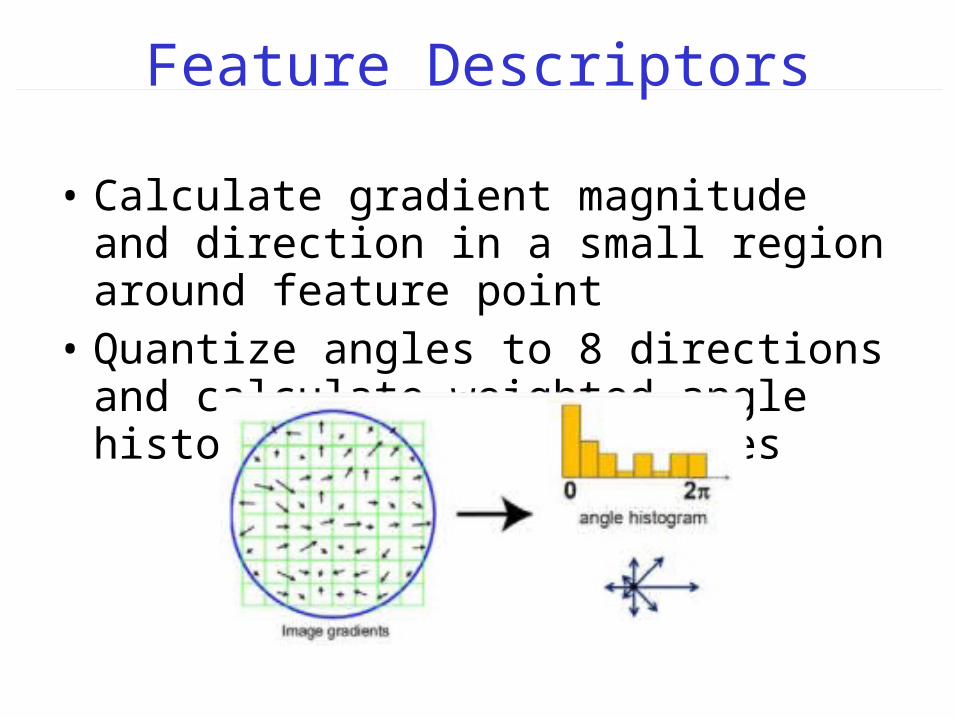
• Calculate gradient magnitude and direction in a small region around feature point

• Quantize angles to 8 directions and calculate weighted angle histogram to get 8 features

Feature Descriptors

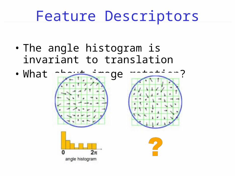
• The angle histogram is invariant to translation• What about image rotation?

Feature Descriptors

• How can we fix this problem? – Find the dominant gradient direction – Rotate the region so the dominant gradient

direction is at angle zero– Recalculate the angle histogram

• We can get almost the same result by shifting the angle histogram to put largest value into the angle zero bucket

Feature Descriptors

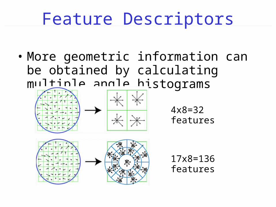
• More geometric information can be obtained by calculating multiple angle histograms

4x8=32 features

17x8=136 features

Feature Descriptors

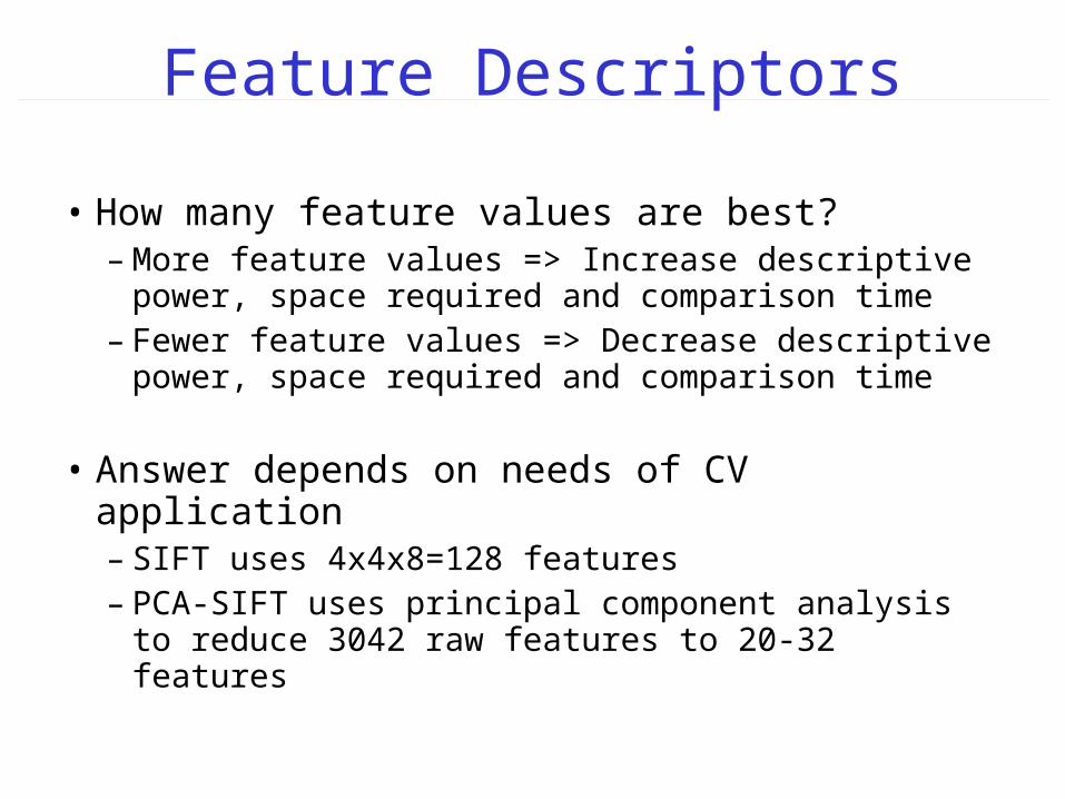
• How many feature values are best?– More feature values => Increase descriptive power,

space required and comparison time– Fewer feature values => Decrease descriptive

power, space required and comparison time

• Answer depends on needs of CV application– SIFT uses 4x4x8=128 features– PCA-SIFT uses principal component analysis to

reduce 3042 raw features to 20-32 features

Feature Matching

• There are two issues in feature matching – Matching strategy - how feature vectors are

compared to each other– Data structures and algorithms - how feature

vectors are stored and retrieved

• We must handle lots of data quickly and get robust and accurate feature matching results

Feature Matching

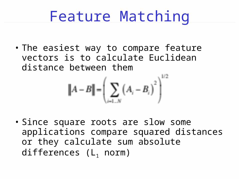
• The easiest way to compare feature vectors is to calculate Euclidean distance between them

• Since square roots are slow some applications compare squared distances or they calculate sum absolute differences (L1 norm)

Feature Matching

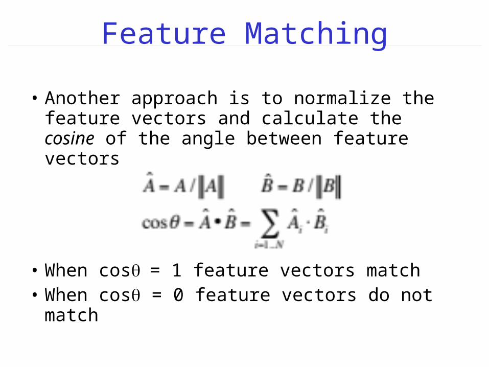
• Another approach is to normalize the feature vectors and calculate the cosine of the angle between feature vectors

• When cos= 1 feature vectors match• When cos = 0 feature vectors do not match

Feature Matching

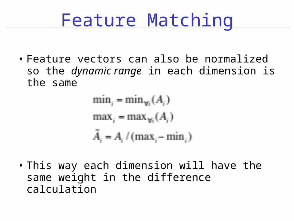
• Feature vectors can also be normalized so the dynamic range in each dimension is the same

• This way each dimension will have the same weight in the difference calculation

Feature Matching

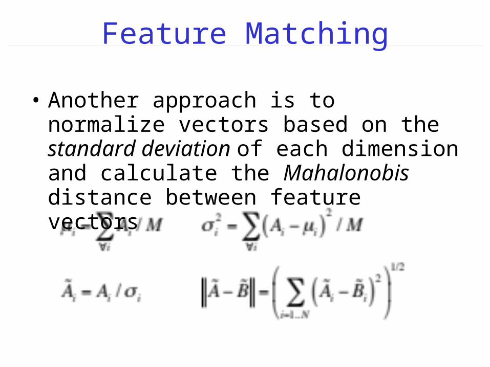
• Another approach is to normalize vectors based on the standard deviation of each dimension and calculate the Mahalonobis distance between feature vectors

Feature Matching

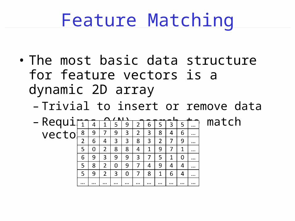
• The most basic data structure for feature vectors is a dynamic 2D array– Trivial to insert or remove data– Requires O(N) search to match vectors

Feature Matching

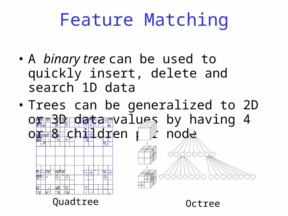
• A binary tree can be used to quickly insert, delete and search 1D data

• Trees can be generalized to 2D or 3D data values by having 4 or 8 children per node

Quadtree Octree

Feature Matching

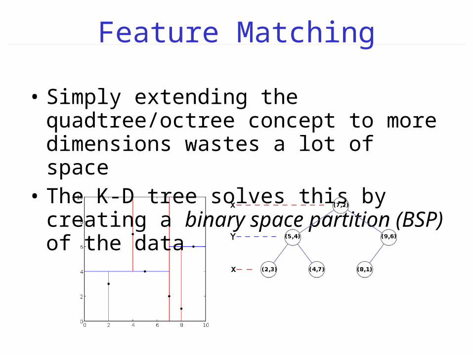
• Simply extending the quadtree/octree concept to more dimensions wastes a lot of space

• The K-D tree solves this by creating a binary space partition (BSP) of the data

Feature Matching

• There are many variations on K-D trees with different BSPs and different search algorithms– Best solutions are O(logN)

• Finally, a number of hash table techniques have been devised to store/search features– Searching is approximate instead of exact– Best solutions are almost constant time

Conclusions

• Goal of feature detection is to find geometric objects in an image that are visually interesting– These features can then be used to create CV

applications for image alignment, object tracking and recognition, and defect detection

• Feature detection and matching is a large area– Different feature detection methods– Different feature descriptors– Different feature matching techniques