chapter 4 –microscopylight.ece.illinois.edu/ece460/pdf/chap xviii - microscopy... ·...

Chapter 4 – Microscopy

Gabriel Popescu

University of Illinois at Urbana‐Champaigny p gBeckman Institute

Quantitative Light Imaging Laboratory

Electrical and Computer Engineering, UIUCPrinciples of Optical Imaging

Quantitative Light Imaging Laboratoryhttp://light.ece.uiuc.edu

4.1 Resolution of Optical Microscopes

ECE 460 – Optical Imaging

The Microscope can be approximated by 2 lenses [ [ [ , ]]]F F U x y


p pp yTube lens

SampleF2’

F2’

Objective[ [ [ , ]]]y

U(x,y)

F’1

[ [ ]]F U x y [ [ [ ]]] [ ]x yF F U U

“‐” sign means inverted image

The objective is the most important part of the microscope

1[ [ , ]]F U x y2 1[ [ [ , ]]] [ , ]yF F U x y U

M M

The objective is the most important part of the microscope

Usually a third lens (ocular) images F2’ at ∞, such that we can visualize it with the relaxed eye.

2Chapter 4: Microscopy



The objective lens dictates the resolution or size of the


jsmallest object that the microscope can resolve.

Contrast is generated by absorption, scattering, etc.

Microscopes can be categorized by the methods that they use to produce contrast.

Let’s consider an infinitely small object (point):Let s consider an infinitely small object (point):

x1 x2xMθ Mθ How small can we see?

ff




Fourier properties of the lens; the reconstructed field is:


p p ;

(4.1)1 12 ( )[ , ] [ , ] i x yU x y U e d d

ξ

We know that and because and

ξ M Mxf

ξM My

f

We can access only a finite frequency range and therefore we can only achieve finite resolution.

We would need an infinite spectrum to reconstruct a

f

We would need an infinite spectrum to reconstruct a d‐function (in this case a point)




Given the finite frequency support we can write:


q y pp

Where

(4.2)[ , ] [ , ] [ , ]U U H 1 i f , 0 t h i{

M M

H ξ ξ

1

0 o t h e r w i s e{Hξ

ξ ξξ

So, eq. 4.1 becomes

(4.3)[ ] [ [ ] [ ]]U x y F U H (4.3)[ , ] [ [ , ] [ , ]]U x y F U H




Use the Convolution Theorem once more (which states that


(convolution in one domain is multiplication in another) to get:

(4.4)[ , ] [ , ] [ , ]U x y U x y h x y V

( )i x y ξ Where is the microscope image

is the ideal image

is the impulse response

[ , ]U x y[ , ]U x y[ ]h x y

( )i x ye ξ

is the impulse response [ , ]h x y

[ , ] [ [ , ]]h x y F H (4.5)

2 2 21 if 0 otherwise[ , ] [ ]x yf f w

x yLH f f circw

p

(4.6) w2w




So, 1

1 w here is a B esse l fu n ctio n o f the 1 st k in d an d o rd er[2 ][ ] , 2

JJ WF H A h

W


,

So the image of a “point” becomes:2 W

22 2 1 [ 2 ][ , ]

2J Wh x y A

W

(4.7)

Since and

2 W

1[ ]2 J xM

MxW

f 2 1.22MW

Hx

so

2x

f

The Airy Function2 1.22Mx

f

61 f so,

A point will be imaged as a smeared spot of diameter

1.22‐1.22

.61M

fx

.61 f

(eq. 4.8)

A point will be imaged as a smeared spot of diameter Mx




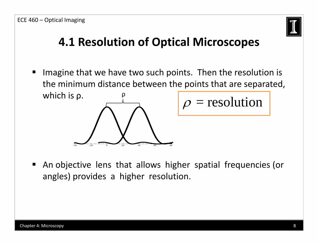
Imagine that we have two such points. Then the resolution is


g pthe minimum distance between the points that are separated, which is ρ. ρ

= resolution

An objective lens that allows higher spatial frequencies (or j g p q (angles) provides a higher resolution.




1Ob 1x 2Ob 2x


1

S

1Mx

S

2Mx2

Definition: 1 1sin tan Mxf

1f 1f

2f 2f

Th l i b b i d h

f

1sin Numerical ApertureNA (4.10)

The resolution becomes but is good enough

Compare Ob1 and Ob2 above:.61

NA 2NA

1 2 1 2 1 2 1 2M Mx x NA NA (4 11)

So Ob2 provides a better resolution.1 2 1 2 1 2 1 2, M Mx x NA NA (4.11)




In general, objectives are made out of several lenses => complex systems


complex systems

'PP

F

fW

ObjectiveEntrance Pupil jfocal distance measured from principal planeworking distance = distance from F to physical surface of lens

Entrance Pupil image of physical aperture

fW

Entrance Pupil = image of physical aperture and entrance pupil determine numerical aperf ture i.e. resolution




Note: if the objective lens is immersed in a medium for which


jn≠1, then

NA n NAn (4.12)

This means that it is possible for immersed objective lenses to have a better resolution.


4.2 Contrast


The final image consists of a distribution which is the [ , ]I x y

4.2 Contrast

gresult of absorption, scattering/diffraction, etc.

Contrast = a measure of the intensity fluctuations across the i I l th t t th b tt

[ , ]y

image. In general, the more contrast the better.

Low Contrast High Contrast

I I

x x12Chapter 4: Microscopy demo available

4.2 Contrast


Microscope image

4.2 Contrast

p g

2 regions of interest: A, B

N is the background noise (in sample) (4.13)

Contrast :

,; = signal A, BAB A B A BC S S S Contrast to noise ratio:

A BABAB

S SCCNR

2

= standard deviation of noise.N N

N

22 ( ) ; = signal in pixelsN i ii

S S S 13Chapter 4: Microscopy

4.2 Contrast


While resolution is given by the instrument, the contrast is

4.2 Contrast

g y ,

given by the instrument/sample combination.

Most biological structures (i.e. cells) are very transparent so

is flat, which means there is low contrast

They can be assumed “phase objects”

[ , ]I x y

Example of a phase object:

100 nm

[ , ]I x y

Imaging system

Wave front

N=1.5

systemk

‐Glass Profile‐Phase Grating



4.2 Contrast

No absorption so [ , ] constant contrast = 0I x y

4.2 Contrast

p

BUT: the wave front carries information about the sample[ , ]y

(4.14)[ , ][ ] i x yE x y E e This is the expression for the field in the vicinity of a phase

object

( )0[ , ]E x y E e

object.

Bright Field microscopy produces low contrast images of phase objectsp j



4.2 Contrast There are several ways to enhance contrast:

Endogeneous Contrast

4.2 Contrast

g Dark field

Phase contrast

Schlerein

Quantitative phase microscopy

Confocal

Endogeneous florescenceg

Exogeneous Contrast Agents Staining

Florescent taggingFull field

Florescent tagging

More recently

Beads (dielectric and metallic)

Nano

Confocal

Nano

Quantum Dots


4.3 Dark Field Microscopy


Consider the low contrast imageI( )


I(x)

x

I(x,y)

Typical low pass filtering = remove ∆C

I(x) I(f ) Remove low I(x)

x

FourierI(fx)

fx

Frequency

Then take the inverse Fourier Transformation

Inverse I(x)Inverse Fourier

I(x)

x

High Contrast




Actual MicroscopeLens


fObject

Lens

Blocks low Enhanced Contrastfrequency

High frequency components are enhanced (eg. edges)( g g )

Without the sample Dark Field


4.4 Schlerein Method


Not used very often nowadaysBlocks ½ Image Plane

4.4 Schlerein Method

spectrumImage Plane

Fourier Inverse Fourier

Enhances Contrast

Phase objects can be rendered visible

Edges are enhanced Edges are enhanced

Relates to Hilbert Transform.19Chapter 4: Microscopy

4.4 Schlieren Method


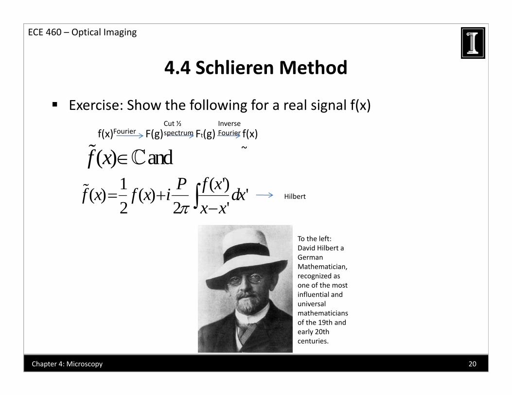
Exercise: Show the following for a real signal f(x)Cut ½ Inverse

4.4 Schlieren Method

f(x) F(g) Ft(g) f(x)FourierCut ½ spectrum

Inverse Fourier

~( ) andf x Hilbert

1 ( ')( ) ( ) '2 2 '

P f xf x f x i dxx x

To the left: David Hilbert a German Mathematician, recognized as one of the most influential and universal mathematicians of the 19th andof the 19th and early 20th centuries.


4.5 Phase Contrast Microscopy


Developed by Frits Zernike (1935) yielding Noble prize in 1953(Physics)


1953(Physics)

Very powerful, commonly used today.

Consider a phase object:Consider a phase object:

Intensity distribution:

( , )( , ) i x yU x y e (4.15)

2( , )1 No Contrast

I x y U

Assume: The microscope has a magnification M=1(x,y) (x’,y’)

Fourier PlaneS Image

plane




2 ( )( , ) ( , ) x yi f fx yU f f U x y e dxdy (4.16)


;

x xx yf ff f

Note:

Central Ordinate Theorem

(0,0) ( , ) U U x y dxdy (4.17)

Zero Frequency component corresponds to a plane wave in the image plane(constant of (x,y))Plane Wave

1( , )U x y dxdy 0

1( , )U U x y dxdy

A




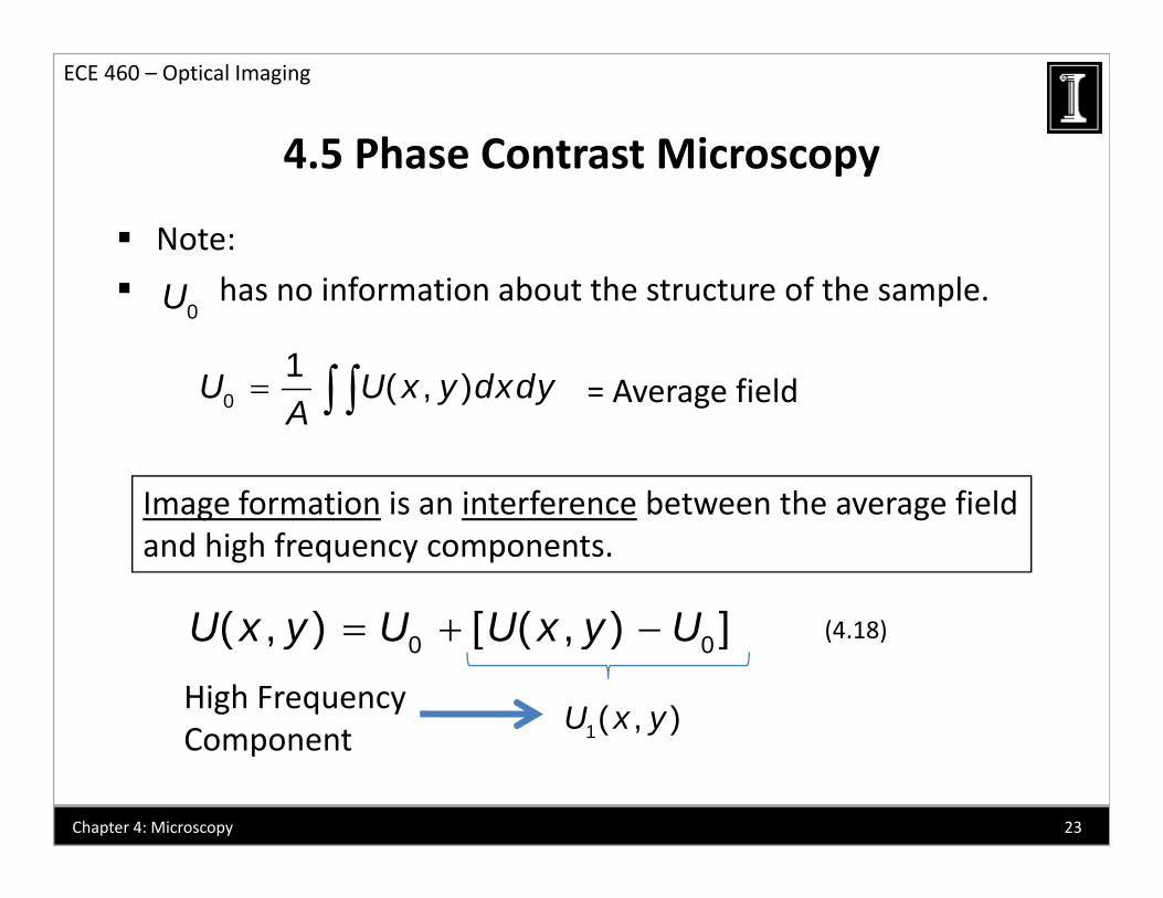
Note:

h i f i b h f h l


has no information about the structure of the sample.

= Average field1

( )U U x y dxdy

0U

= Average field

Image formation is an interference between the average field

0 ( , )U U x y dxdyA

Image formation is an interference between the average field and high frequency components.

( ) [ ( ) ]U x y U U x y U

High Frequency C t

0 0( , ) [ ( , ) ]U x y U U x y U

1( , )U x y

(4.18)

Component 1( , )y




Phase contrast relies on shifting the phase of by 0U


0 0iU U ae

Assume ; becomes:

The intensity distribution in the image plane0 1U 0 0

iU U ae

0 0

( , ) [ ( , ) 1]iU x y ae U x y

(4 19) The intensity distribution in the image plane becomes:

2( , ) ( , )I x y U x y

(4.19)

2( , )

2 ( )

1

1 1 Re[2 2 2 ]

i i x y

i i i

ae e

a ae ae e

2

[ ]2[1 cos cos cos( )]a a a (4.20)




Note: For a = 0 recover Dark Field Microscopy

Assume “small” phase shift


Assume small phase shift

cos 1;2

2

2

2

( , ) 2 sin sin2 ( , ) sin

I x y a aa a x y

PC couples into intensity

a<1 enhances contrast (best modulation for )

2( , ) 2 ( , )I x y a a x y (4.21)

U U a<1 enhances contrast (best modulation for ) 0 1U U


4.6 Nomarski/Differential Interference Contrast i


DIC= Differential Interference Contrast

Microscopy

11

Condenser

x

Movable Wollaston

P

11

11

0 0 0

SS

Wollaston Prism #1 Wollaston Prism #2

Obj.

Use polarization discrimination to create 2 interfering Use polarization discrimination to create 2 interfering beams

Illuminate sample(s) with 2 drifted beamsp ( )




“Shift” amount Airy disk2NA

Microscopy

Wollaston prism #2 brings the 2 beams together through i t f

2NA

interference.

011 0 1 0

iiTotalE E E A e A e (4.22)

l

. l d

d

dl

.

1 0 1 0cosdn k n d k




By varying the position of Wollaston prism

Microscopy

one can adjust Phase Shift through the sample:

1 0

dx

l

.

x

z

( )i x dxe

( )i xe

S

becomes:

0

0 11 0

( )0

( )0 [1 ]

ni iTotal n

i i

E A e A e

A e e

(4.23)0 [ ]e e




The Intensity in the image plane (as a function of

Microscopy

displacement x).

f

0( ) 2 (1 cos[ ( ) ( ) ])I x I x dx x (4.24)

Note: For small , best results obtained for

0( ) 2 (1 sin[ ( ) ( )])I x I x dx x

2

S h fi l i i di ib i i l d h di

0( ) ( )2 [1 ]x dx xI dx

dx

(4.25)

So the final intensity distribution is related to the gradient of the phase: ( )x

x




DIC is a very sensitive to edges, even though the actual

Microscopy

phase shifts are “small”.

Example:sample

I t it

x

Intensity no contrast

x

x

Ph t t d DIC h il d t d i ll f Phase contrast and DIC heavily used today, especially for investigating live biological structures (cells) noninvasively.


4.7 Quantitative Phase Microscopy


PC &DIC are great, but qualitative in terms of phase

K i i i l ff d i

4.7 Quantitative Phase Microscopy

Knowing quantitatively offers some advantages, i.e. gives a map of structure density; for homogeneous structures, gives molecular information.

( , )x y

QPM is a “rather new” domain; several methods so far.

Main obstacle is noise


4.8 Confocal Microscopy


So far, we discussed full‐ field imaging, i.e obtaining the entire image at once(great feature: imaging as a parallel


entire image at once(great feature: imaging as a parallel process).

The image can be recorded point by point also(like TV), sometimes with some advantages.

Confocal = same focal point for illumination and collection

Pinhole




Due to pinhole, light out of focus is rejected, which can create stacks of slices hence 3D rendering


create stacks of slices, hence 3D rendering

Scanning: either by scanning the sample or the beam

Note:Note:

3D Info

large field of view (limited by aperture)

up to better resolution

! It works in reflection usuallyBS2

Pinhole


4.8 Confocal Microscopy/ NSOM


Recent development: Multi Foci

I i i i i


Improves acquisition time

Need more power Trade‐off

Multiple Focused beam

Confocal can provide many frames/seconds(video rate)

Leading to 4D imaging(x,y,z,t)





Near Field Scanning Optical Microscope(NSOM)

C i i f f l & AFM Continuation of confocal & AFM

Tappered fiber as cantilever :

FiberAperture down to 50 nm

Evanescent waves (no transmission in air)


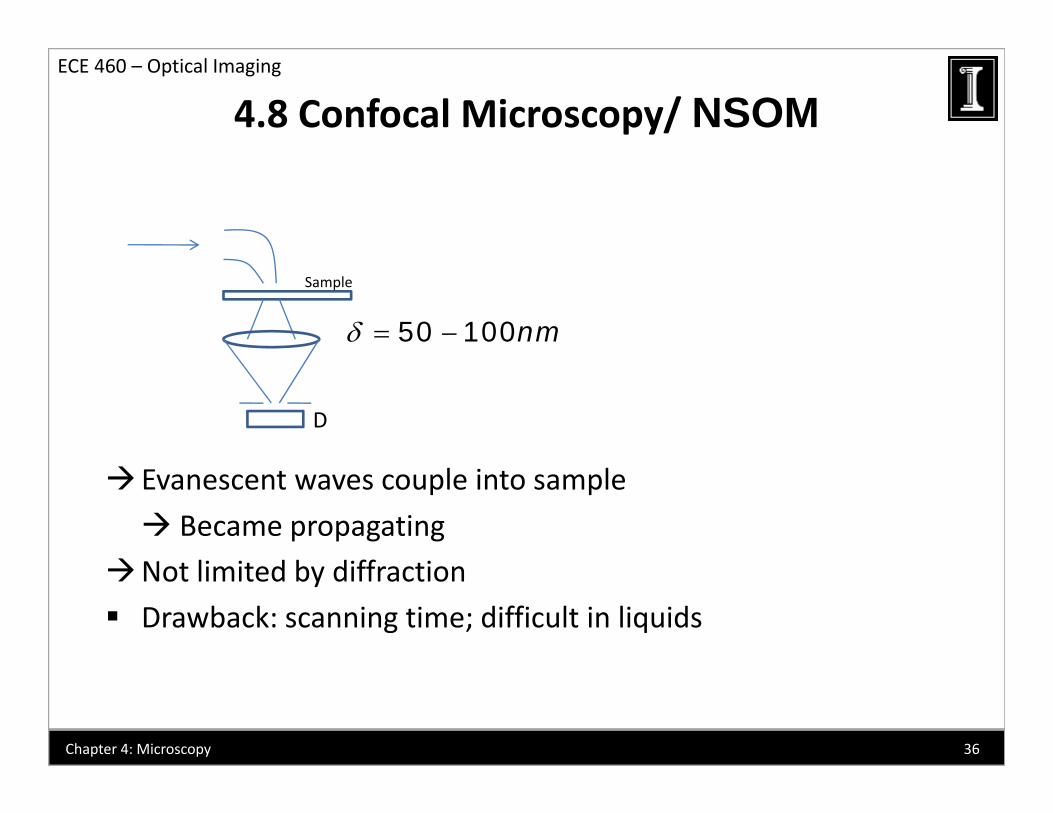
4.8 Confocal Microscopy/ NSOMECE 460 – Optical Imaging

Sample

50 100nm

D

Evanescent waves couple into sample

Became propagating l d b d ffNot limited by diffraction

Drawback: scanning time; difficult in liquids


4.9 Fluorescence Microscopy


Illumination and emission have different wavelengths


Endogenous “Fluorophoress” eg. NADH

Most commonly exogenous

Recently:

GFP technology (given fluorescent protein)

genetically encoded fused with DNA genetically encoded, fused with DNA

GFP live cell imaging

allows for multiple “fluorophores”allows for multiple fluorophores

dynamic monitoring of processes(cell signaling)




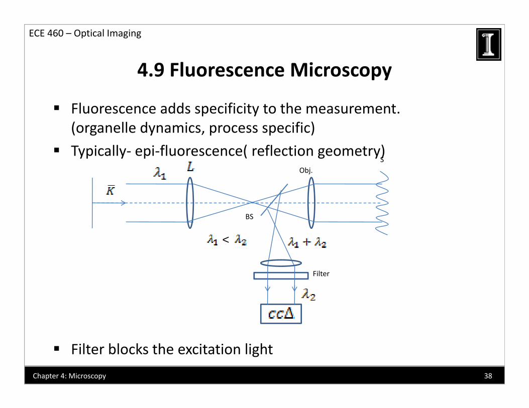
Fluorescence adds specificity to the measurement. (organelle dynamics process specific)


Obj.S

(organelle dynamics, process specific)

Typically‐ epi‐fluorescence( reflection geometry)

BS

Filter

<

Filter blocks the excitation light




Full‐Field is limited to thin samples

Combine fluorescence & confocal leads to deeper penetration


Combine fluorescence & confocal leads to deeper penetration

Issues when imaging live cells:

acquisition time, sensitivity, damage.

Photo‐bleaching can produce cell damage:

limit duration of illumination need efficiency sensitivityi ifi d CCD use intensified CCD

Acquisition speed: improve with multi‐foci &Nipkow disk scanning




Other Fluorescence Techniques:

T l i l fl i


Total internal reflection

FCS‐Fluorescence correlation spectroscopy

FRAP‐Fluorescence recovery after photobleaching FRAP‐Fluorescence recovery after photobleaching

FRET‐Fluorescence resonance energy transfer.

FLIM‐fluorescence lifetime imaging.g g

STED‐Stimulated emission depletion 100nm spot STED+ 4Pi confocal microscopy 33nm diffraction spot

single molecule imaging.

PALM, fPALM

Fiona etc Fiona, etc


4.10 Multiphoton Imaging


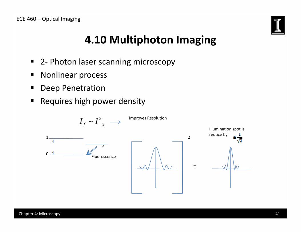
2‐ Photon laser scanning microscopy

N li


Nonlinear process

Deep Penetration

Requires high power density Requires high power density

Improves Resolution

Illumination spot is

2f xI I

z

1

0Fluorescence

2

preduce by

=





2nd harmonic Imaging‐recent:

E d SHG l l ( ll ) Endogenous SHG molecules(e.g collagen)

coherent process (phase matching)

Same advantage of smaller illumination spot

( ) 2 LP E Same advantage of smaller illumination spot

Let’s take a look at examples!


Microscopy imagesMicroscopy images

http://www.microscopyu.com/NikonNikon

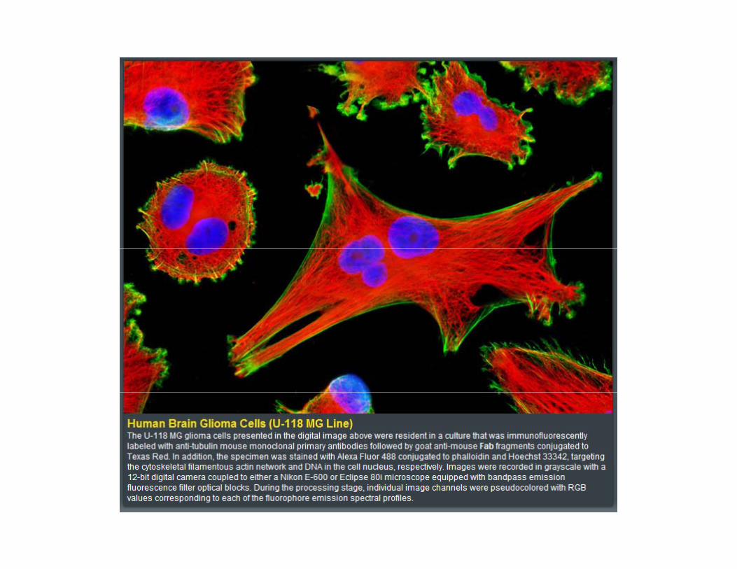
1. Cell imaging

Fluorescence microscopymicroscopy

http://www.microscopyu.com/Nikon

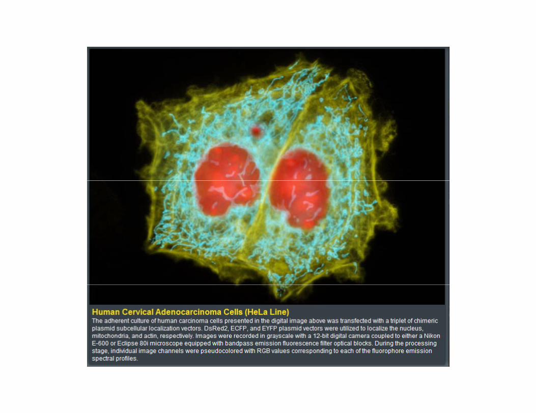
2. Tissue slice imaging

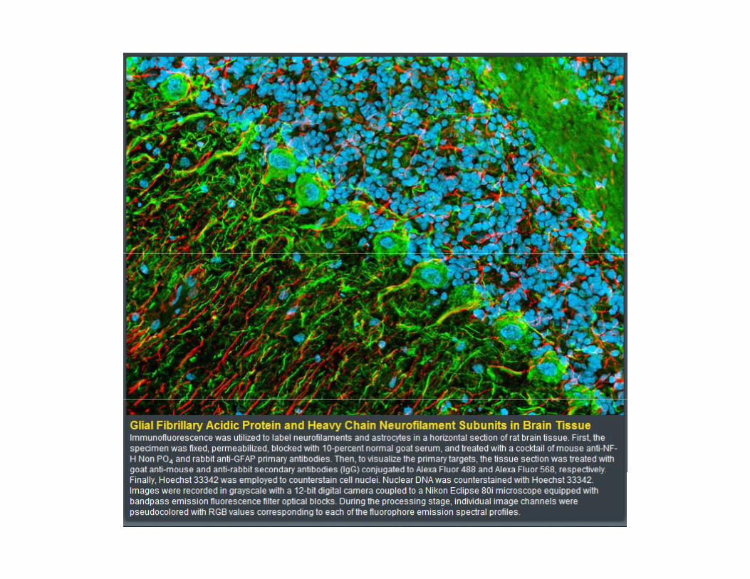
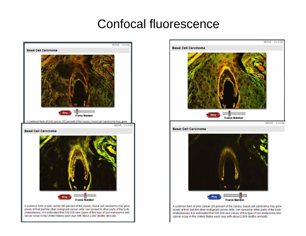
Confocal fluorescence

chapter 4 –microscopylight.ece.illinois.edu/ece460/pdf/chap xviii - microscopy... ·...

Documents