Random Variables

ECE460Spring, 2012

2

CombinatoricsNotation:

Population size

Subpopulation size

Ordered Sample

How many samples of size r can be formed from a population of size n?

1 2 3 3 1 2, , , ,a a a a a a

n

r

1. Sampling with replacement and ordering

2. Sampling without replacement and with ordering

3

How many samples of size r can be formed from a population of size n?

3. Sampling without replacement and without ordering

4. Sampling with replacement and without ordering

4

Bernoulli TrialsIndependent trials that result in a success with probability p any failure probability 1-p.

5

Conditional ProbabilitiesGiven two events, E1 & E2, defined on the same probability space with corresponding probabilities P(E1) & P(E2):

1 2

21 2 2

, 0( | )

0, Otherwise

P E EP E

P E E P E

6

Example 4.5An information source produces 0 and 1 with probabilities 0.3 and 0.7, respectively. The output of the source is transmitted via a channel that has a probability of error (turning a 1 into a 0 or a 0 into a 1) of 0.2.1. What is the probability that at the output a 1 is observed?2. What is the probability that a 1 was the output of the source if at

the output of the channel a 1 is observed?

7

Random VariablesWorking with Sets has its limitations

– Selecting events in Ω– Assigning P[ ]– Verification of 3 Axioms

Would like to leave set theory and move into more advanced & widely used mathematics(i.e., Integration, Derivatives, Limits…)

Random Variables:– Maps sets in Ω to R– Subsets of the real line

of the form arecalled Borel sets. A collection of Borel sets is called a Borel σ-fields.

– A function that will associate events in Ω with the Borel sets is called a Random Variable.

1. 0

2. 1

3. if

P E

P

P E F P E P F E F

( , ]x

8

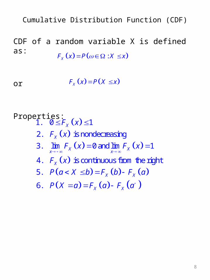
Cumulative Distribution Function (CDF)

CDF of a random variable X is defined as:

or

Properties:

:XF x P X x

XF x P X x

1. 0 1

2. is nondecreasing

3. lim 0 and lim 1

4. is continuous from the right

5.

6.

X

X

X Xx x

X

X X

X X

F x

F x

F x F x

F x

P a X b F b F a

P X a F a F a

9

Probability Density Function (PDF)

PDF of a random variable X is defined as:

Properties:

For discrete random variables, this is known as the Probability Mass Function (PMF)

X X

df x F x

dx

1. 0

2. 1

3.

4. In general,

5.

X

X

b

Xa

XA

x

X X

f x

f x dx

f x dx P a X b

P X A f x dx

F x f u du

i ip P X x

10

Example 4.6A coin is flipped three times and the random variable X denotes the total number of heads that show up. The probability of a head in one flip of this coin is denoted by p.1. What values can the random variable X take?2. What is the PMF of the random variable X?3. Derive and plot the CDF of X.4. What is the probability that X exceeds 1?

11

Uniform Random VariableThis a continuous random variable taking values between a and b with equal probabilities over intervals of equal length.

12

Bernoulli Random VariableOnly two outcomes (e.g., Heads or Tails)

Probability Mass Function:

Leads to binomial law (sampling w/o replacement & w/o ordering)

Example: 10 independent, binary pulses per second arrive at a receiver. The error probability (that is, a zero received as a one or vice versa) is 0.001. What is the probability of at least one error/second?

1 , 0

[ ] , 1

0, otherwise

p x

P X x p x

successes in trials ; ,

where = probability of a success

P k n b k n p

p

13

Binomial Law ExampleFive missiles are fired against an aircraft carrier in the ocean. It takes at least two direct hits to sink the carrier. All five missiles are on the correct trajectory must get through the “point defense” guns of the carrier. It is known that the point defense guns can destroy a missile with probability P = 0.9. What is the probability that the carrier will still be afloat after the encounter?

14

Uniform Distribution

Probability Density Function (pdf)

Cumulative distribution function

A resistor r is an RV uniform distribution between 900 and 1100 ohms. Find the probability that r is between 950 and 1050 ohms.

a bx

1

b a

15

Gaussian (Normal) Random VariableA continuous random variable described by the density function:

Properties:

2( )

221

2

x m

Xf x e

Notation: : ,X N m

2

1. If where and are scalars,

then : ,

2.0,1

3. a

X X

Y aX b a b

Y N a m b a

x mN

F a f x dx

16

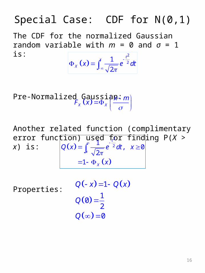
Special Case: CDF for N(0,1)The CDF for the normalized Gaussian random variable with m = 0 and σ = 1 is:

Pre-Normalized Gaussian:

Another related function (complimentary error function) used for finding P(X > x) is:

Properties:

2

21

2

tx

X x e dt

1

10

20

Q x Q x

Q

Q

2

21

, 02

1

t

x

X

Q x e dt x

x

X X

x mF x

17

Gaussian ExampleA random variable is N(1000; 2500). Find the probability that x is between 900 and 1050.

18

Complimentary Error Function

19

The Central Limit TheoremLet be a set of random variables with the following properties:

1. The Xk with k = 1, 2, …, n are statistically independent

2. The Xk all have the same probability density function

3. Both the mean and the variance exist for each Xk

Let Y be a new random variable defined as

The, according to the central limit theorem, the normalized random variable

Approaches a Gaussian random variable with zero mean and unit variance as the number of random variables Increases without limit.

1 2, ,..., nX X X

1

n

kk

Y X

[ ]

Y

Y E YZ

1 2, ,..., nX X X

20

Functions of Random VariablesLet X be a r.v. with known CDF and PDF. If g(X) is a function of the r.v. X then

Example:Given the function where a > 0 and b are constants and X is a r.v. withFind

:Y

X iY

i i

Y g X

F y P g X y

f xf y

g x

Y aX b

and .Y YF y f y .XF x

21

Statistical AveragesThe expected value of the random variable X is defined as

Special Cases:

Characteristic Functions:

Special Cases:

XE g x g x f x dx

j xX Xf x e dx

22

Multiple Random VariablesThe joint CDF of X and Y is

and its joint PDF is

Properties:

, , : ,

,

X YF x y P X x Y y

P X x Y y

2

, ,, ,X Y X Yf x y F x yx y

, ,

, ,

,

,,

, ,

1. , , ,

2. , , ,

3. , 1

4. , ,

5. , ,

X X Y Y X Y

X X Y Y X Y

X Y

X Yx y A

x y

X Y X Y

F x F x F y F y

f x f x y dy f y f x y dx

f x y dx dy

P X Y A f u v du dv

F x y f u v dv du

23

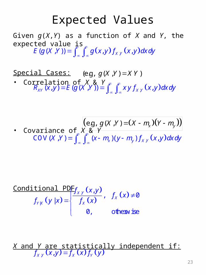
Expected ValuesGiven g(X,Y) as a function of X and Y, the expected value is

Special Cases:• Correlation of X & Y

• Covariance of X & Y

Conditional PDF

X and Y are statistically independent if:

,( ( , )) , ,X YE g X Y g x y f x y dx dy

(e.g, ( , ) )g X Y X Y

,( , ) ( ( , )) ,XY X YR x y E g X Y x y f x y dx dy

e.g, ( , ) x yg X Y X m Y m

,COV( , ) ( )( ) ,x y X YX Y x m y m f x y dx dy

,

|

,, 0

|

0, otherwise

X YX

Y X X

f x yf x

f y x f x

, ,X Y X Yf x y f x f y

24

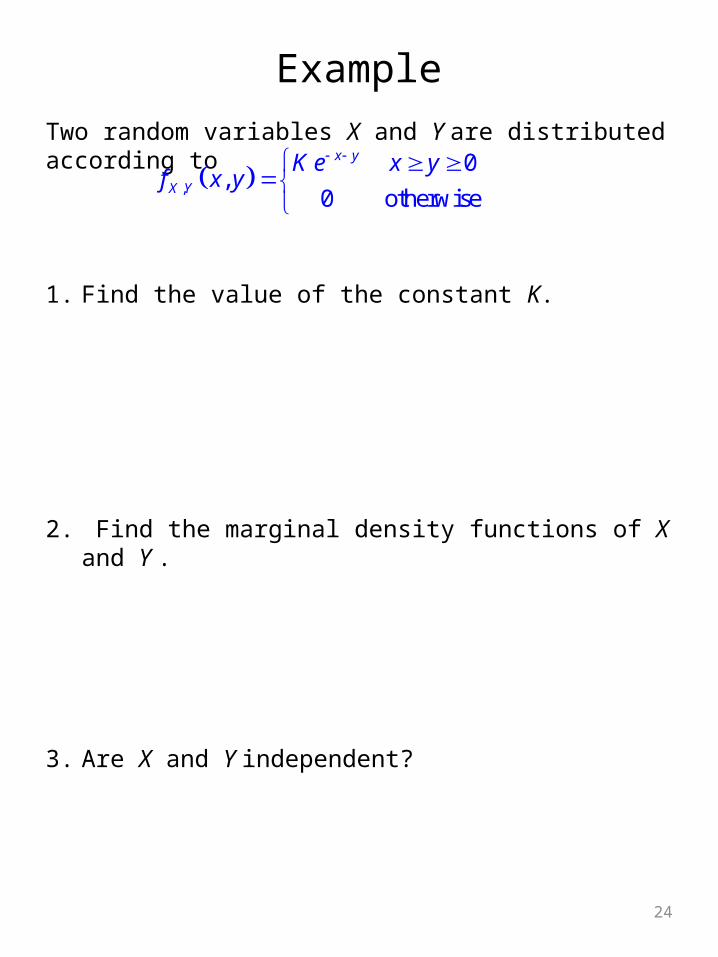
ExampleTwo random variables X and Y are distributed according to

1. Find the value of the constant K.

2. Find the marginal density functions of X and Y .

3. Are X and Y independent?

,

0,

0 otherwise

x y

X Y

K e x yf x y

25

Example4. Find

5. Find

6. Find

| | .X Yf x y

| .E X Y y

,COV , and .X YX Y

26

Jointly Gaussian R.V.’sDefinition: X and Y are jointly Gaussian if

where ρ is the correlation coefficient between X and Y. If ρ = 0, then

If jointly Gaussian, then the following are also Gaussian

, 221 2

2 2

1 2 1 22 21 2 1 2

1 1, exp

2 12 1

2

X Yf x y

x m y m x m y m

| |, , ,X Y ff x f y x y f y x

, ,X Y X Yf x y f x f y

27

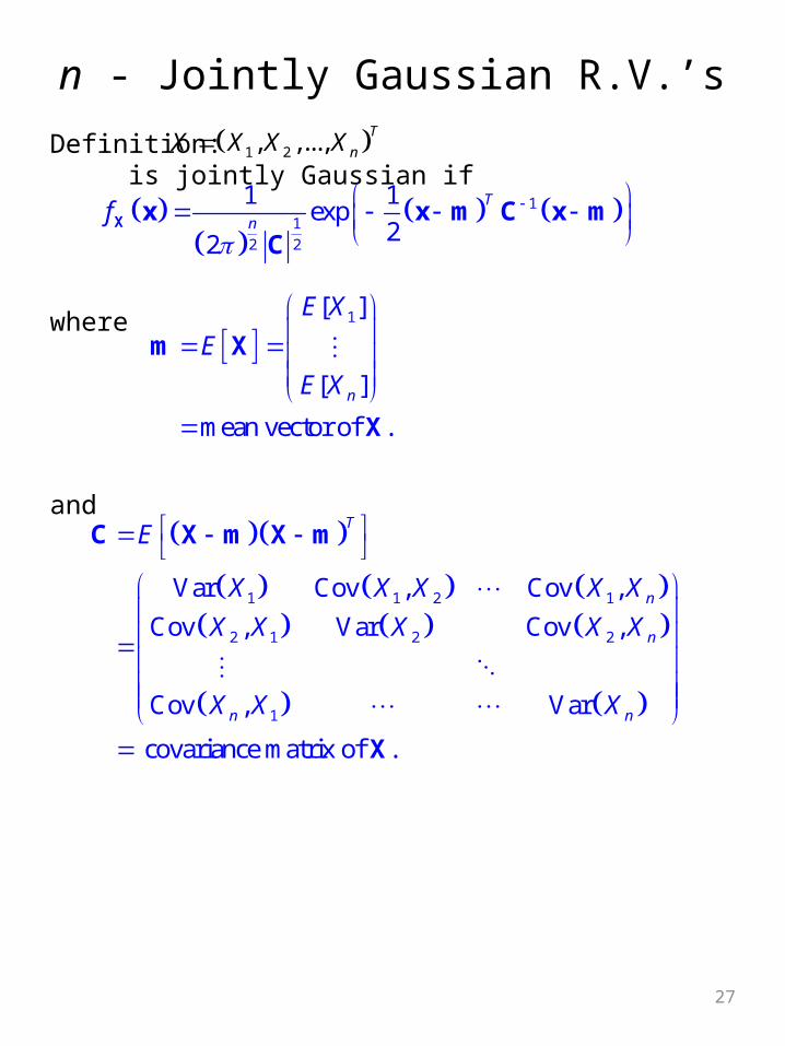
n - Jointly Gaussian R.V.’sDefinition: is jointly Gaussian if

where

and

1 2, ,...,T

nX X X X

11

22

1 1exp

22

T

nf

X x x m C x mC

1[ ]

[ ]

mean vector of .n

E X

E

E X

m X

X

1 1 2 1

2 1 2 2

1

Var Cov , Cov ,

Cov , Var Cov ,

Cov , Var

covariance matrix of .

T

n

n

n n

E

X X X X X

X X X X X

X X X

C X m X m

X

28

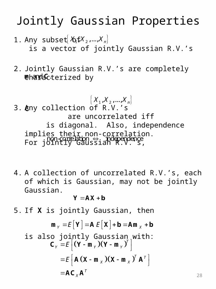
Jointly Gaussian Properties1. Any subset of is a vector of jointly Gaussian

R.V.’s

2. Jointly Gaussian R.V.’s are completely characterized by

3. Any collection of R.V.’s are uncorrelated iff is diagonal. Also, independence implies their non-correlation.For jointly Gaussian R.V.’s,

4. A collection of uncorrelated R.V.’s, each of which is Gaussian, may not be jointly Gaussian.

5. If X is jointly Gaussian, then

is also jointly Gaussian with:

and .m C

1 2, ,..., nX X X

1 2, ,..., nX X XC

non-correlation independence

Y AX b

Y XE E m Y A X b Am b

T

Y Y Y

T TX X

TX

E

E

C Y m Y m

A X m X m A

AC A

29

Example

Let A be a binary random variable that takes the values of +1 and -1 with equal probabilities. Let A and X are statistically independent. Let Y = A X.

1. Find the pdf

2. Find the covariance cov(X,Y).

3. Find the covariance cov(X2,Y2).

4. Are X and Y jointly Gaussian?

2~ 0, .X N

.Yf y