Chapter 3: Cluster Analysis

3.1 Basic Concepts of Clustering 3.2 Partitioning Methods 3.3 Hierarchical Methods

3.3.1 The Principle

3.3.2 Agglomerative and Divisive Clustering

3.3.3 BIRCH

3.3.4 Rock 3.4 Density-based Methods

3.4.1 The Principle

3.4.2 DBSCAN

3.4.3 OPTICS 3.5 Clustering High-Dimensional Data 3.6 Outlier Analysis

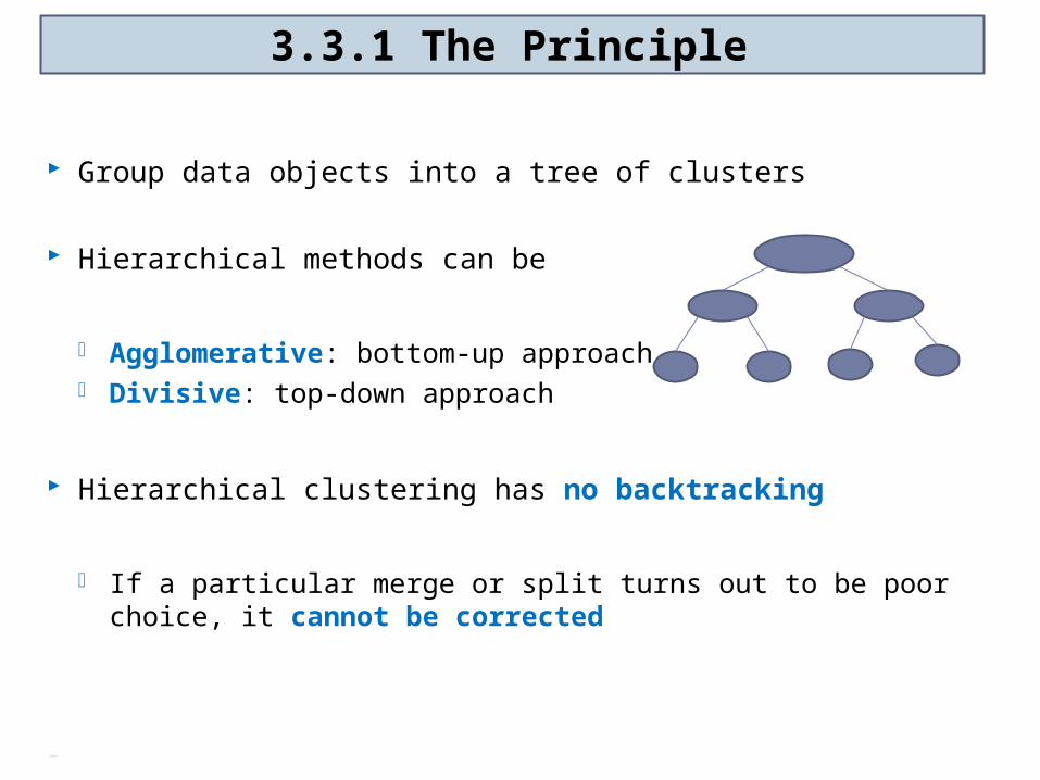
3.3.1 The Principle

Group data objects into a tree of clusters

Hierarchical methods can be

Agglomerative: bottom-up approach Divisive: top-down approach

Hierarchical clustering has no backtracking

If a particular merge or split turns out to be poor choice, it cannot be corrected

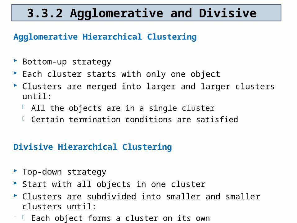
3.3.2 Agglomerative and Divisive

Agglomerative Hierarchical Clustering

Bottom-up strategy Each cluster starts with only one object Clusters are merged into larger and larger clusters until:

All the objects are in a single cluster Certain termination conditions are satisfied

Divisive Hierarchical Clustering

Top-down strategy Start with all objects in one cluster Clusters are subdivided into smaller and smaller clusters until:

Each object forms a cluster on its own Certain termination conditions are satisfied

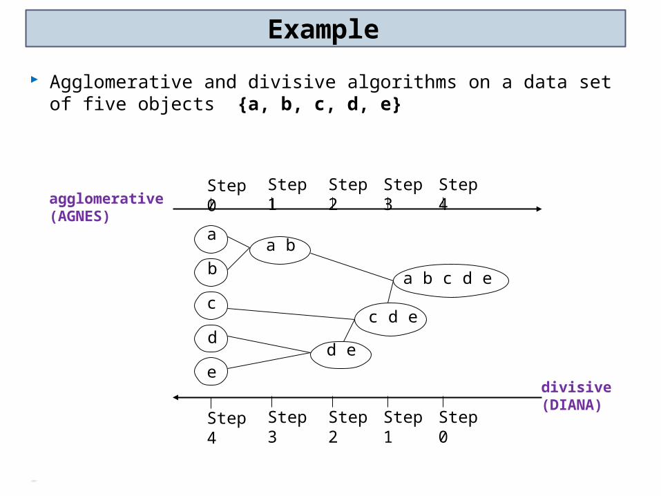
Example

Agglomerative and divisive algorithms on a data set of five objects {a, b, c, d, e}

Step 0 Step 1 Step 2 Step 3 Step 4

b

d

c

e

aa b

d e

c d e

a b c d e

Step 4 Step 3 Step 2 Step 1 Step 0

agglomerative(AGNES)

divisive(DIANA)

Example

AGNES

Clusters C1 and C2

may be merged if an object

in C1 and an object in C2 form

the minimum Euclidean

distance between any two

objects from different clusters

DIANA

A cluster is split according to some principle, e.g., the maximum Euclidian distance between the closest neighboring objects in the cluster

Step 0 Step 1 Step 2 Step 3 Step 4

b

d

c

e

aa b

d e

c d e

a b c d e

Step 4 Step 3 Step 2 Step 1 Step 0

agglomerative(AGNES)

divisive(DIANA)

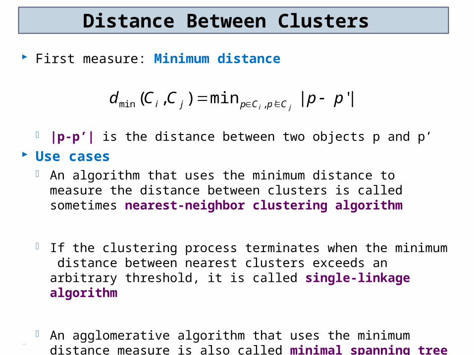
Distance Between Clusters

First measure: Minimum distance

|p-p’| is the distance between two objects p and p’ Use cases

An algorithm that uses the minimum distance to measure the distance between clusters is called sometimes nearest-neighbor clustering algorithm

If the clustering process terminates when the minimum distance between nearest clusters exceeds an arbitrary threshold, it is called single-linkage algorithm

An agglomerative algorithm that uses the minimum distance measure is also called minimal spanning tree algorithm

|'|min),( ',min ppCCdji CpCpji

Distance Between Clusters

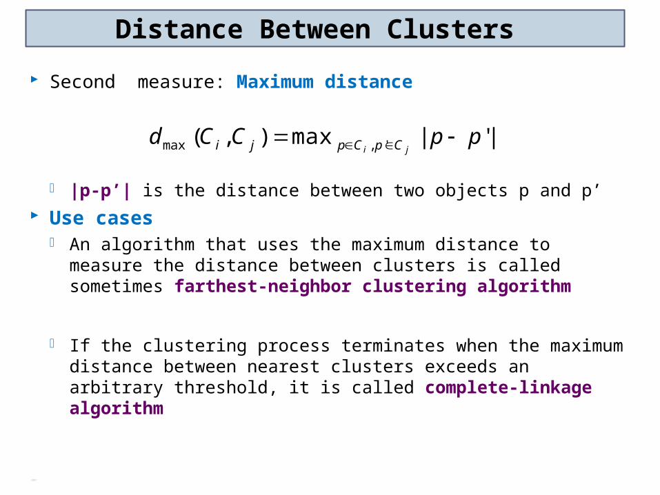
Second measure: Maximum distance

|p-p’| is the distance between two objects p and p’ Use cases

An algorithm that uses the maximum distance to measure the distance between clusters is called sometimes farthest-neighbor clustering algorithm

If the clustering process terminates when the maximum distance between nearest clusters exceeds an arbitrary threshold, it is called complete-linkage algorithm

|'|max),( ',max ppCCdji CpCpji

Distance Between Clusters

Minimum and maximum distances are extreme implying that they are overly sensitive to outliers or noisy data

Third measure: Mean distance

mi and mj are the means for cluster Ci and Cj respectively

Fourth measure: Average distance

|p-p’| is the distance between two objects p and p’ ni and nj are the number of objects in cluster Ci and Cj

respectively Mean is difficult to compute for categorical data

||),( jijimean mmCCd

i jCp Cpji

jiavg ppnn

CCd'

|'|1

),(

Challenges & Solutions

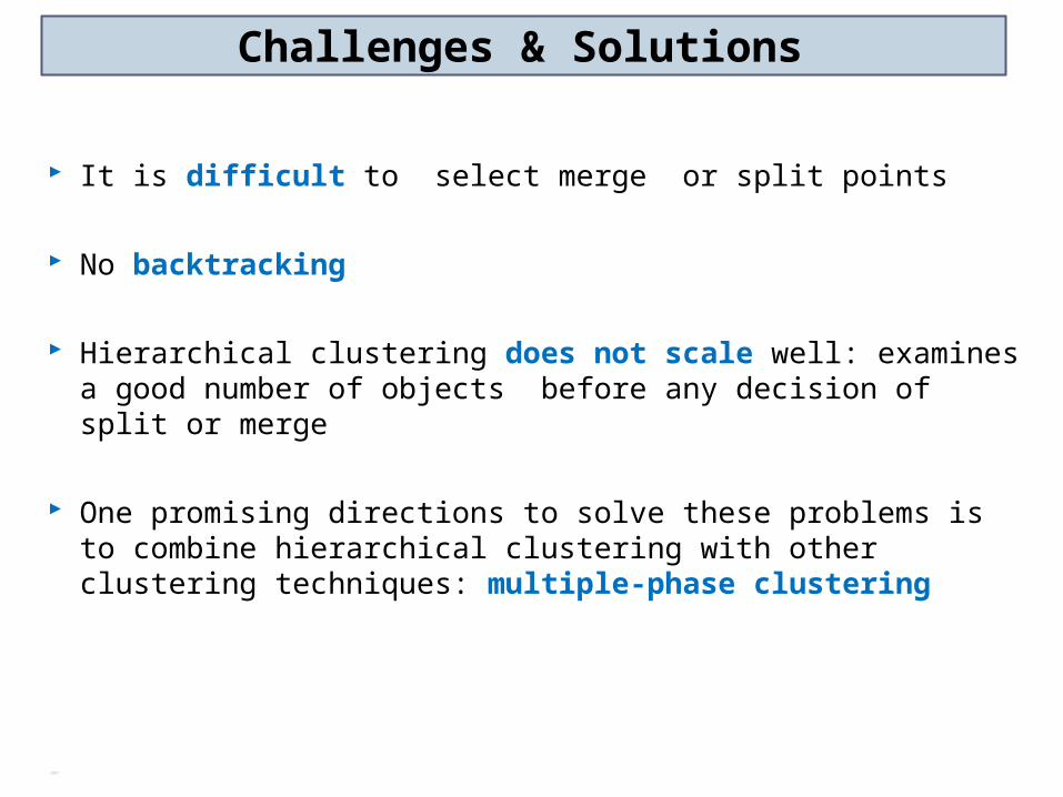
It is difficult to select merge or split points

No backtracking

Hierarchical clustering does not scale well: examines a good number of objects before any decision of split or merge

One promising directions to solve these problems is to combine hierarchical clustering with other clustering techniques: multiple-phase clustering

3.3.3 BIRCH

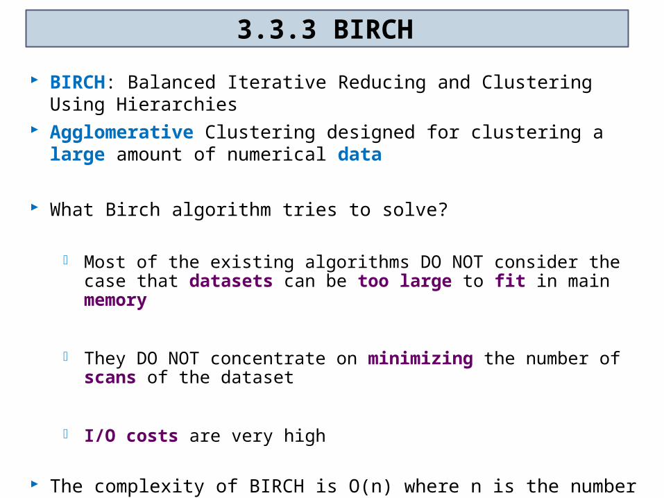
BIRCH: Balanced Iterative Reducing and Clustering Using Hierarchies

Agglomerative Clustering designed for clustering a large amount of numerical data

What Birch algorithm tries to solve?

Most of the existing algorithms DO NOT consider the case that datasets can be too large to fit in main memory

They DO NOT concentrate on minimizing the number of scans of the dataset

I/O costs are very high

The complexity of BIRCH is O(n) where n is the number of objects to be clustered.

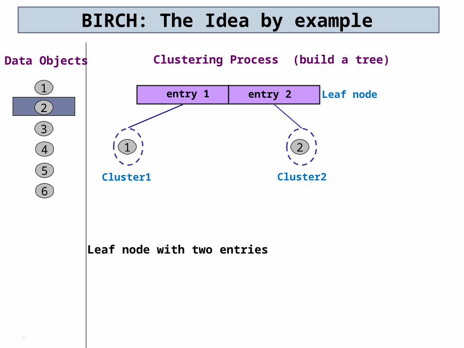
BIRCH: The Idea by example

Data Objects

1

Clustering Process (build a tree)

Cluster1

1

2

3

4

5

6

2

If cluster 1 becomes too large (not compact) by adding object 2,then split the cluster

Leaf node

BIRCH: The Idea by example

Data Objects

1

Clustering Process (build a tree)

Cluster1

1

2

3

4

5

6

2

Leaf node

Cluster2

entry 1 entry 2

Leaf node with two entries

BIRCH: The Idea by example

Data Objects

1

Clustering Process (build a tree)

Cluster1

1

2

3

4

5

6

2

Leaf node

Cluster2

3

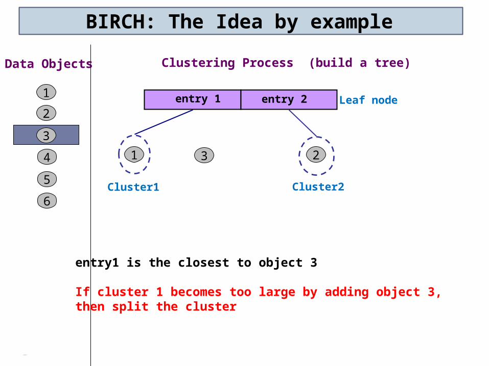
entry1 is the closest to object 3

If cluster 1 becomes too large by adding object 3,then split the cluster

entry 1 entry 2

BIRCH: The Idea by example

Data Objects

1

Clustering Process (build a tree)

Cluster1

1

2

3

4

5

6

2

Leaf node

Cluster2

3

entry 1 entry 2 entry 3

Cluster3

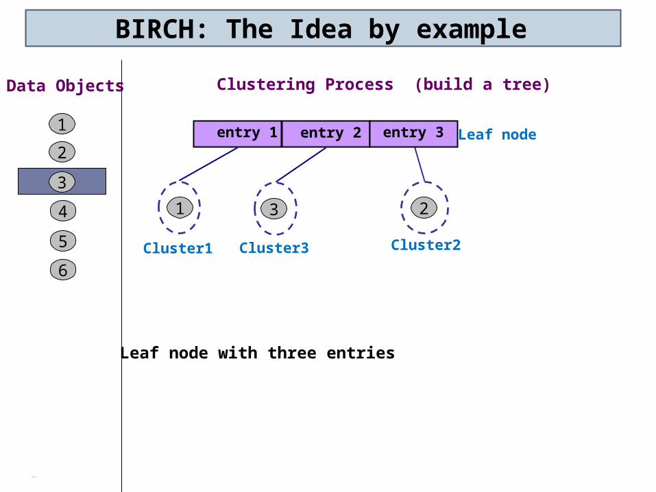
Leaf node with three entries

BIRCH: The Idea by example

Data Objects

1

Clustering Process (build a tree)

Cluster1

1

2

3

4

5

6

2

Leaf node

Cluster2

3

entry 1 entry 2 entry 3

Cluster3

4

entry3 is the closest to object 4

Cluster 2 remains compact when adding object 4then add object 4 to cluster 2

Cluster2

BIRCH: The Idea by example

Data Objects

1

Clustering Process (build a tree)

Cluster1

1

2

3

4

5

6

2

Leaf node

3

entry 1 entry 2 entry 3

Cluster3

4

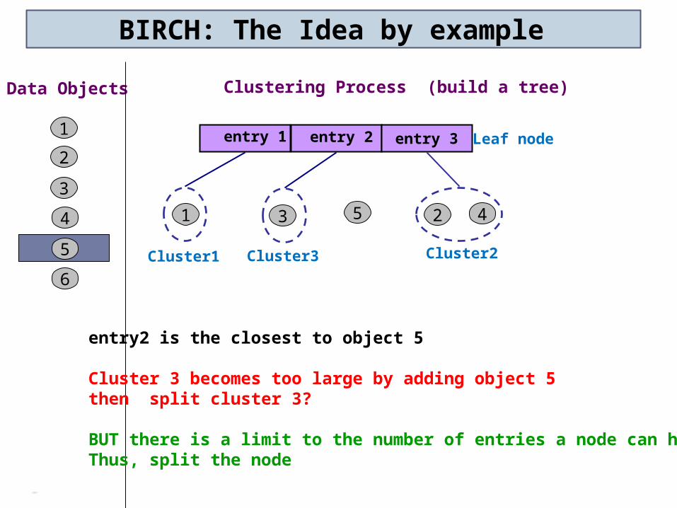
entry2 is the closest to object 5

Cluster 3 becomes too large by adding object 5then split cluster 3?

BUT there is a limit to the number of entries a node can haveThus, split the node

Cluster2

5

BIRCH: The Idea by example

Data Objects

1

Clustering Process (build a tree)

Cluster1

1

2

3

4

5

6

2

Leaf node

3

Cluster3

4

Cluster2

5

entry 1 entry 2

entry 1.1 entry 1.2 entry 2.1 entry 2.2

Leaf node

Non-Leaf node

Cluster4

BIRCH: The Idea by example

Data Objects

1

Clustering Process (build a tree)

Cluster1

1

2

3

4

5

6

2

Leaf node

3

Cluster3

4

Cluster2

5

entry 1 entry 2

entry 1.1 entry 1.2 entry 2.1 entry 2.2

Leaf node

Non-Leaf node

Cluster4

6

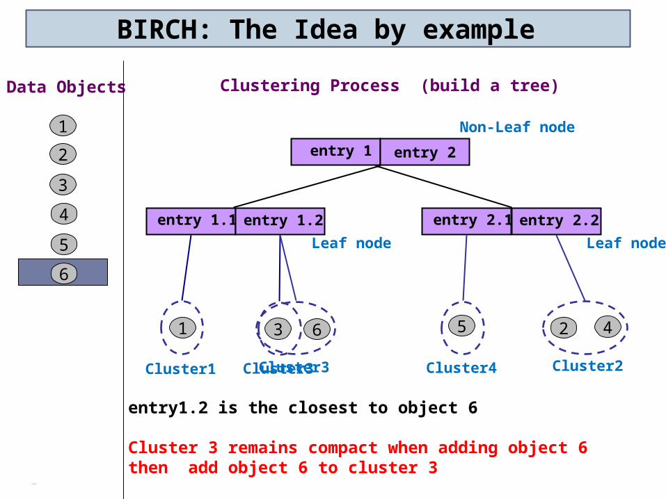
entry1.2 is the closest to object 6

Cluster 3 remains compact when adding object 6then add object 6 to cluster 3

Cluster3

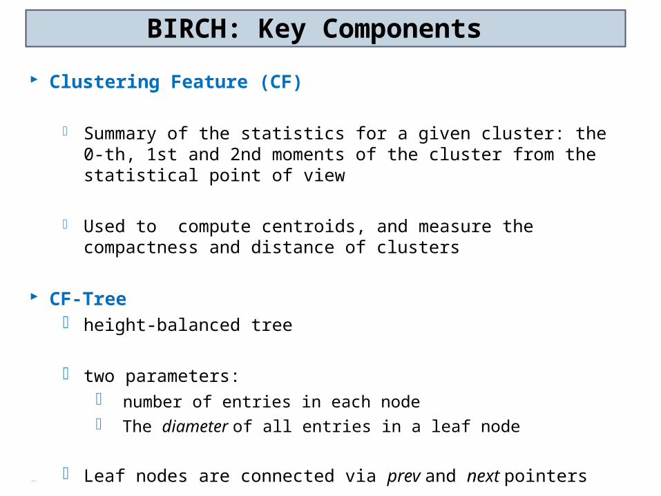
BIRCH: Key Components

Clustering Feature (CF)

Summary of the statistics for a given cluster: the 0-th, 1st and 2nd moments of the cluster from the statistical point of view

Used to compute centroids, and measure the compactness and distance of clusters

CF-Tree height-balanced tree

two parameters: number of entries in each node The diameter of all entries in a leaf node

Leaf nodes are connected via prev and next pointers

Clustering Feature

Clustering Feature (CF): CF = (N, LS, SS)

N: Number of data points

LS: linear sum of N points:

SS: square sum of N points:

N

i iX1

N

i iX1

2

Cluster 1 (2,5) (3,2) (4,3)

CF2= 3, (35,36), (417 ,440)

Cluster 2

CF1= 3, (2+3+4 , 5+2+3), (22+32+42 , 52+22+32) = 3, (9,10), (29 ,38)

Cluster3

CF3=CF1+CF2= 3+3, (9+35, 10+36), (29+417 , 38+440) = 6, (44,46), (446 ,478)

Properties of Clustering Feature

CF entry is a summary of statistics of the cluster

A representation of the cluster

A CF entry has sufficient information to calculate the centroid, radius, diameter and many other distance measures

Additively theorem allows us to merge sub-clusters incrementally

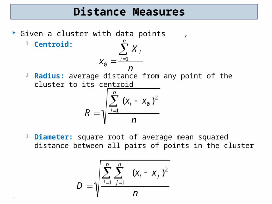
Distance Measures

Given a cluster with data points , Centroid:

Radius: average distance from any point of the cluster to its centroid

Diameter: square root of average mean squared distance between all pairs of points in the cluster

n

Xx

n

ii

10

n

xxR

n

ii

1

20 )(

n

xx

D

n

iji

n

j

1

2

1

)(

CF Tree

B = Branching Factor,

maximum children

in a non-leaf node T = Threshold for

diameter or radius

of the cluster in a leaf L = number of entries in

a leaf CF entry in parent = sum of CF entries of a child of that entry

In-memory, height-balanced tree

CF1 CF2

… CFk

CF1 CF2

… CFk

… …

… … …

Root level

Firstlevel

CF Tree Insertion

Start with the root

Find the CF entry in the root closest to the data point, move to that child and repeat the process until a closest leaf entry is found.

At the leaf

If the point can be accommodated in the cluster, update the entry

If this addition violates the threshold T, split the entry, if this violates the limit imposed by L, split the leaf. If its parent node is full, split that and so on

Update the CF entries from the leaf to the root to accommodate this point

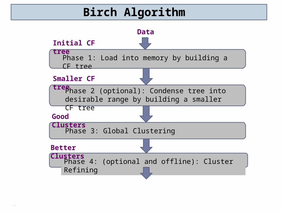
Phase 1: Load into memory by building a CF tree

Phase 2 (optional): Condense tree into desirable range by building a smaller CF tree

Initial CF tree

Data

Phase 3: Global Clustering

Smaller CF tree

Good Clusters

Phase 4: (optional and offline): Cluster Refining

Better Clusters

Birch Algorithm

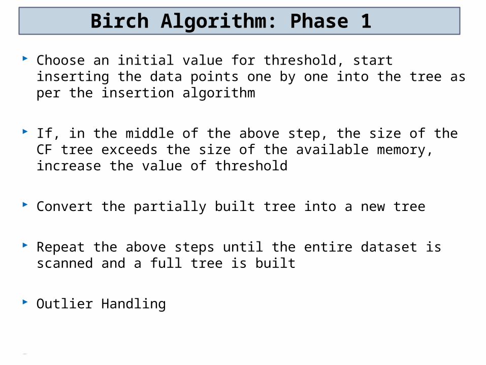
Birch Algorithm: Phase 1

Choose an initial value for threshold, start inserting the data points one by one into the tree as per the insertion algorithm

If, in the middle of the above step, the size of the CF tree exceeds the size of the available memory, increase the value of threshold

Convert the partially built tree into a new tree

Repeat the above steps until the entire dataset is scanned and a full tree is built

Outlier Handling

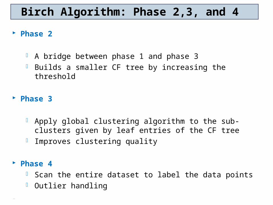
Birch Algorithm: Phase 2,3, and 4

Phase 2

A bridge between phase 1 and phase 3 Builds a smaller CF tree by increasing the threshold

Phase 3

Apply global clustering algorithm to the sub-clusters given by leaf entries of the CF tree

Improves clustering quality

Phase 4 Scan the entire dataset to label the data points Outlier handling

3.3.4 ROCK: for Categorical Data

Experiments show that distance functions do not lead to high quality clusters when clustering categorical data

Most clustering techniques assess the similarity between points to create clusters

At each step, points that are similar are merged into a single cluster

Localized approach prone to errors

ROCK: uses links instead of distances

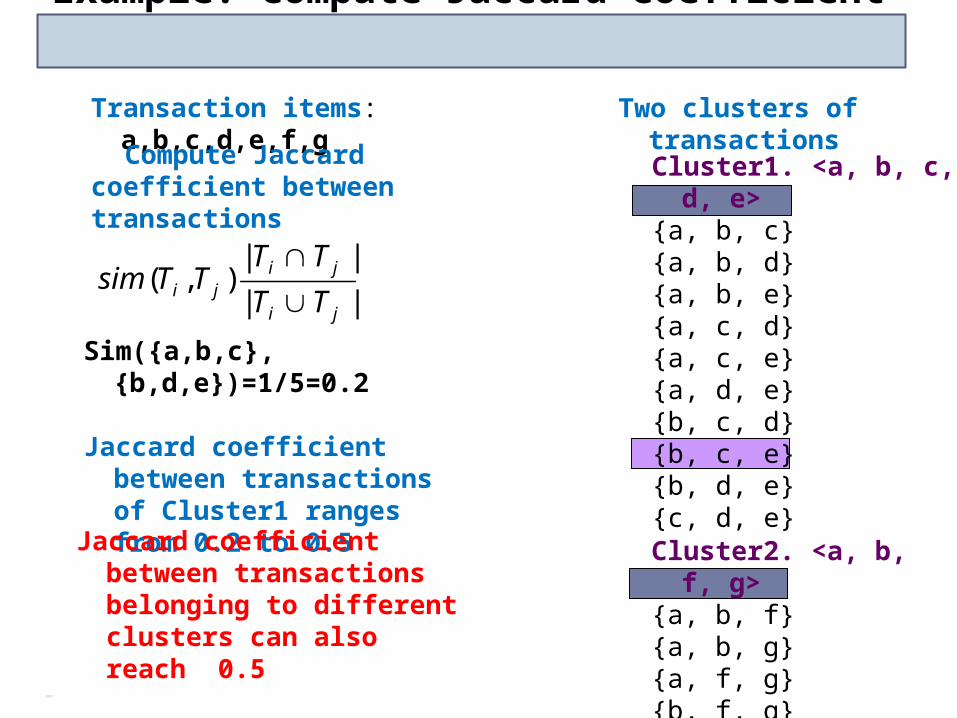
Example: Compute Jaccard Coefficient Transaction items:

a,b,c,d,e,f,gTwo clusters of

transactions Compute Jaccard coefficient between transactions

||

||),(

ji

jiji TT

TTTTsim

Sim({a,b,c},{b,d,e})=1/5=0.2

Jaccard coefficient between transactions of Cluster1 ranges from 0.2 to 0.5

Cluster1. <a, b, c, d, e>

{a, b, c}{a, b, d}{a, b, e}{a, c, d}{a, c, e}{a, d, e}{b, c, d}{b, c, e}{b, d, e}{c, d, e}Cluster2. <a, b, f,

g>{a, b, f}{a, b, g}{a, f, g}{b, f, g}

Jaccard coefficient between transactions belonging to different clusters can also reach 0.5

Sim({a,b,c},{a,b,f})=2/4=0.5

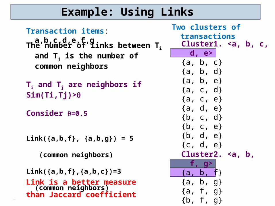
Example: Using Links Transaction items:

a,b,c,d,e,f,g

Two clusters of transactions

The number of links between Ti and Tj is the number of common neighbors

Ti and Tj are neighbors if Sim(Ti,Tj)>

Consider =0.5

Link({a,b,f}, {a,b,g}) = 5 (common neighbors)

Link({a,b,f},{a,b,c})=3 (common neighbors)

Cluster1. <a, b, c, d, e>

{a, b, c}{a, b, d}{a, b, e}{a, c, d}{a, c, e}{a, d, e}{b, c, d}{b, c, e}{b, d, e}{c, d, e}Cluster2. <a, b,

f, g>{a, b, f}{a, b, g}{a, f, g}{b, f, g}

Link is a better measure

than Jaccard coefficient

ROCK

ROCK: Robust Clustering using linKs

Major Ideas Use links to measure similarity/proximity Not distance-based Computational complexity

ma: average number of neighbors

mm: maximum number of neighbors

n: number of objects

Algorithm Sampling-based clustering Draw random sample Cluster with links Label data in disk

O n nm m n nm a( log )2 2

Chapter 3: Cluster Analysis

3.1 Basic Concepts of Clustering 3.2 Partitioning Methods 3.3 Hierarchical Methods

3.3.1 The Principle

3.3.2 Agglomerative and Divisive Clustering

3.3.3 BIRCH

3.3.4 Rock 3.4 Density-based Methods

3.4.1 The Principle

3.4.2 DBSCAN

3.4.3 OPTICS 3.5 Clustering High-Dimensional Data 3.6 Outlier Analysis

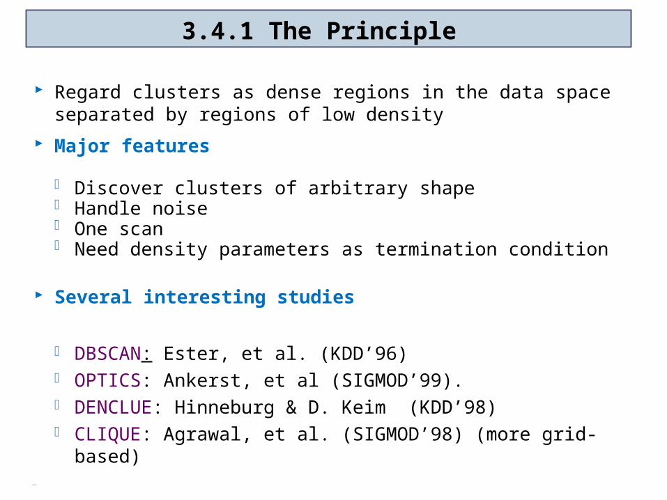
3.4.1 The Principle

Regard clusters as dense regions in the data space separated by regions of low density

Major features

Discover clusters of arbitrary shape Handle noise One scan Need density parameters as termination condition

Several interesting studies

DBSCAN: Ester, et al. (KDD’96) OPTICS: Ankerst, et al (SIGMOD’99). DENCLUE: Hinneburg & D. Keim (KDD’98) CLIQUE: Agrawal, et al. (SIGMOD’98) (more grid-based)

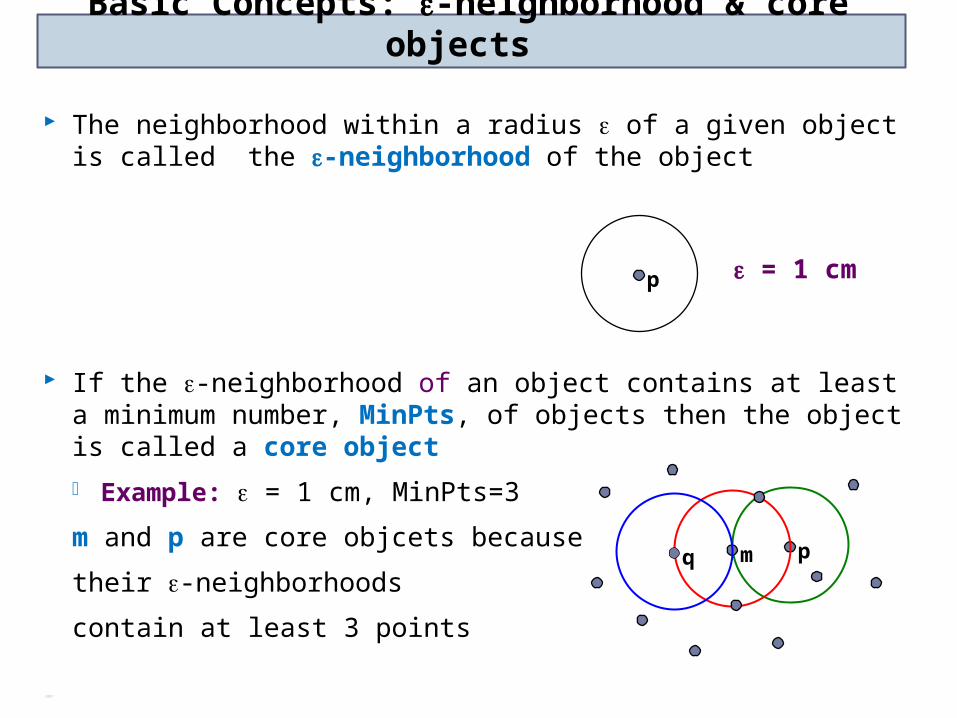
Basic Concepts: -neighborhood & core objects

= 1 cm

The neighborhood within a radius of a given object is called the -neighborhood of the object

If the -neighborhood of an object contains at least a minimum number, MinPts, of objects then the object is called a core object

Example: = 1 cm, MinPts=3

m and p are core objcets because

their -neighborhoods

contain at least 3 points

p

pmq

Directly density-Reachable Objects

An object p is directly density-reachable from object q if p is within the -neighborhood of q and q is a core object

Example:

q is directly density-reachable from m m is directly density-reachable from p and vice versa

pmq

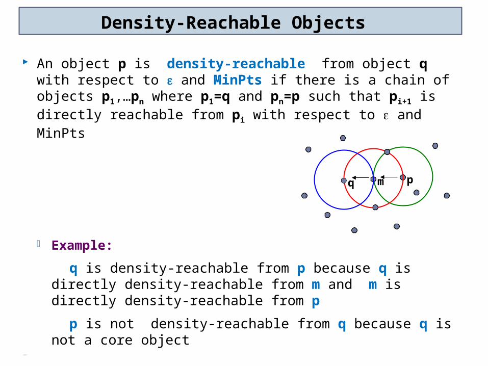
Density-Reachable Objects

An object p is density-reachable from object q with respect to and MinPts if there is a chain of objects p1,…pn where p1=q and pn=p such that pi+1 is directly reachable from pi with respect to and MinPts

Example:

q is density-reachable from p because q is directly density-reachable from m and m is directly density-reachable from p

p is not density-reachable from q because q is not a core object

pmq

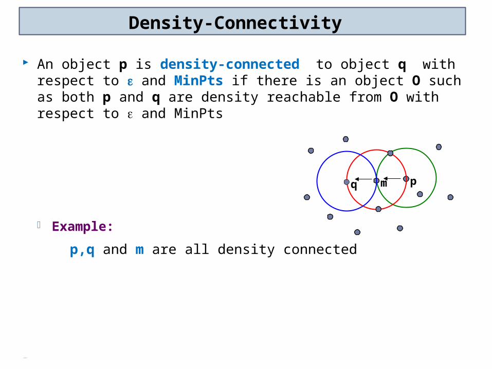
Density-Connectivity

An object p is density-connected to object q with respect to and MinPts if there is an object O such as both p and q are density reachable from O with respect to and MinPts

Example:

p,q and m are all density connected

pmq

3.4.2 DBSCAN

Searches for clusters by checking the -neighborhood of each point in the database

If the -neighborhood of a point p contains more than MinPts, a new cluster with a core object is created

DBSCAN iteratively collects directly density reachable objects from these core objects. Which may involve the merge of a few density-reachable clusters

The process terminates when no new point can be added to any cluster

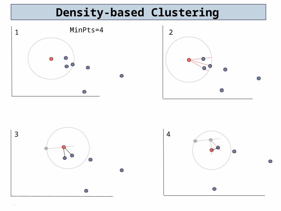
Density-based Clustering

1 2

3 4

MinPts=4

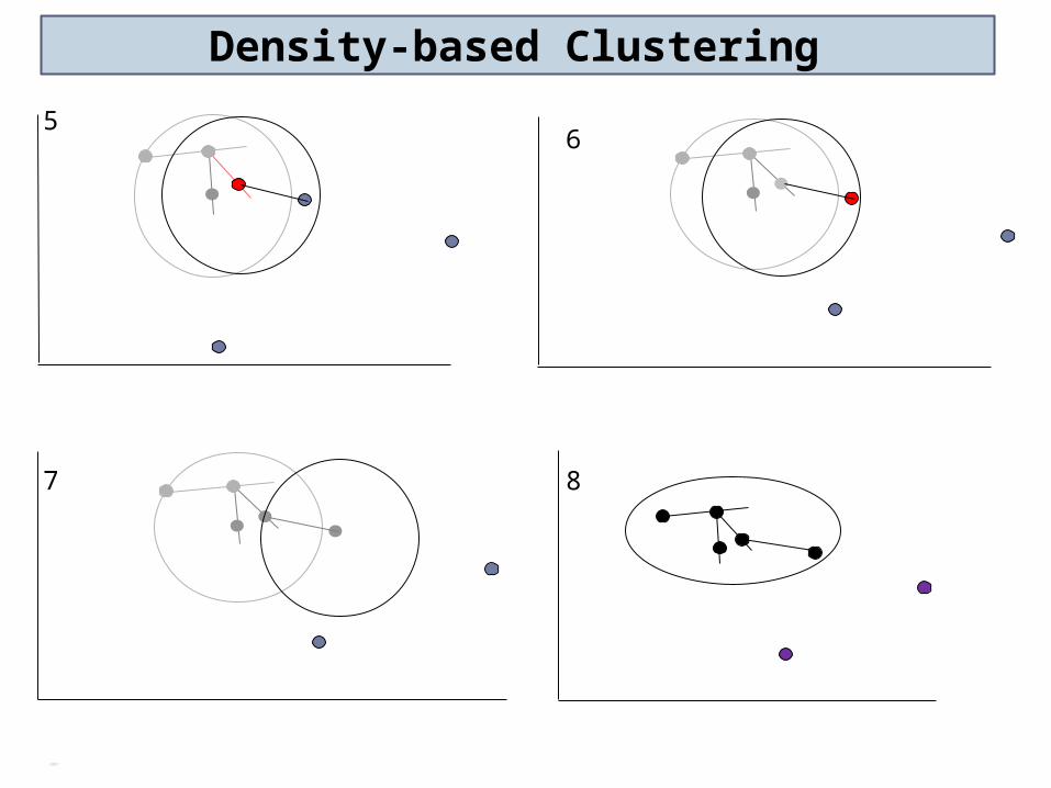
Density-based Clustering

56

7 8

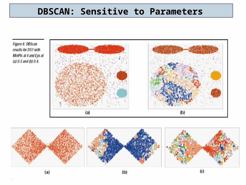
DBSCAN: Sensitive to Parameters

3.4.3 OPTICS

Motivation

Very different local densities may be needed to reveal clusters in different regions

Clusters A,B,C1,C2, and C3 cannot be detected using one global density parameter

A global density parameter can detect either A,B,C or C1,C2,C3

Solutions Use OPTICS

A B

C C1

C2

C3

OPTICS Principle

Produce a special order of the database with respect to its density-based clustering structure

contain information about every clustering level of the data set (up to a generating distance )

Which information to use?

’

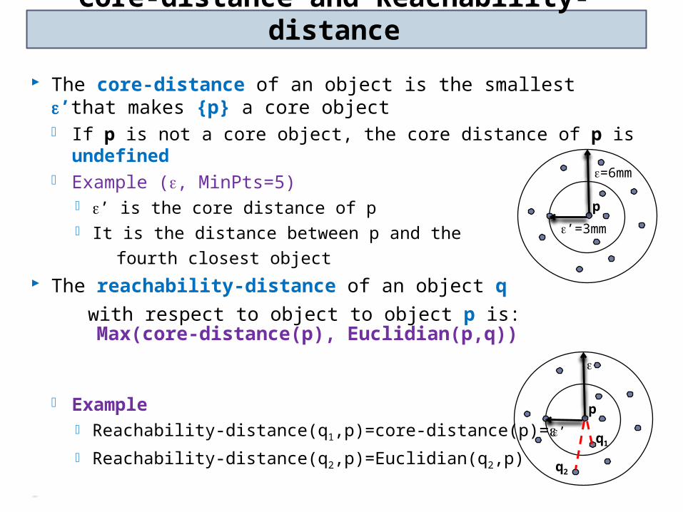
Core-distance and Reachability-distance

The core-distance of an object is the smallest ’that makes {p} a core object If p is not a core object, the core distance of p is undefined Example (, MinPts=5)

’ is the core distance of p It is the distance between p and the

fourth closest object The reachability-distance of an object q

with respect to object to object p is:

Example Reachability-distance(q1,p)=core-distance(p)= Reachability-distance(q2,p)=Euclidian(q2,p)

=6mm

’=3mm

p

’

p

q1

q2

Max(core-distance(p), Euclidian(p,q))

OPTICS Algorithm

Creates an ordering of the objects in the database and stores for each object its:

Core-distance

Distance reachability from the closest core object from which an object have been directly density-reachable

This information is sufficient for the extraction of all density-based clustering with respect to any distance ’ that is smaller than used in generating the order

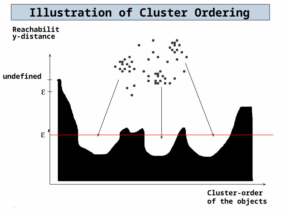
Illustration of Cluster Ordering

Reachability-distance

Cluster-orderof the objects

undefined

’