Chapter 23: Inferences About Means

AP Statistics

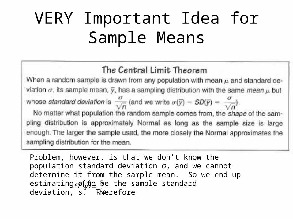
VERY Important Idea for Sample Means

Problem, however, is that we don’t know the population standard deviation σ, and we cannot determine it from the sample mean. So we end up estimating σ to be the sample standard deviation, s. Therefore

n

sySE

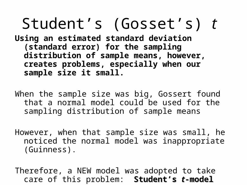
Student’s (Gosset’s) t Using an estimated standard deviation (standard error)

for the sampling distribution of sample means, however, creates problems, especially when our sample size it small.

When the sample size was big, Gossert found that a normal model could be used for the sampling distribution of sample means

However, when that sample size was small, he noticed the normal model was inappropriate (Guinness).

Therefore, a NEW model was adopted to take care of this problem: Student’s Student’s tt-model-model

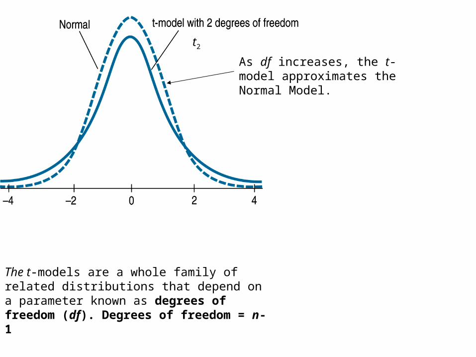
The t-models are a whole family of related distributions that depend on a parameter known as degrees of freedom (df). Degrees of freedom = n-1

As df increases, the t-model approximates the Normal Model.

t2

t-distribution

When we have sample means and do not know the population standard deviation, we use the t-distribution.

We now find t-scores and find the area under the t-model.

Basically, acts like the Normal Model

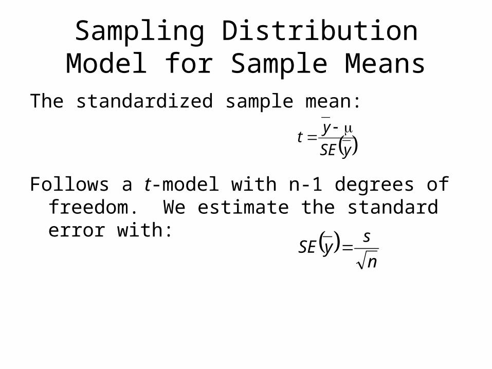
Sampling Distribution Model for Sample Means

The standardized sample mean:

Follows a t-model with n-1 degrees of freedom. We estimate the standard error with:

ySE

yt

n

sySE

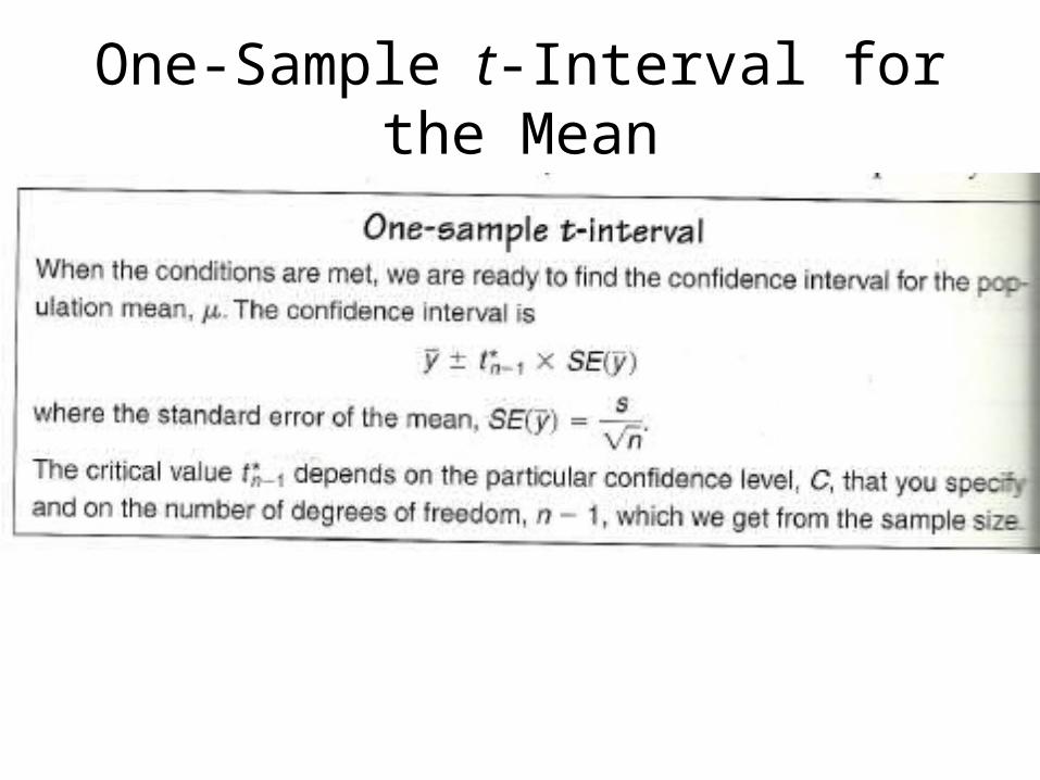
One-Sample t-Interval for the Mean

Assumptions/Conditions

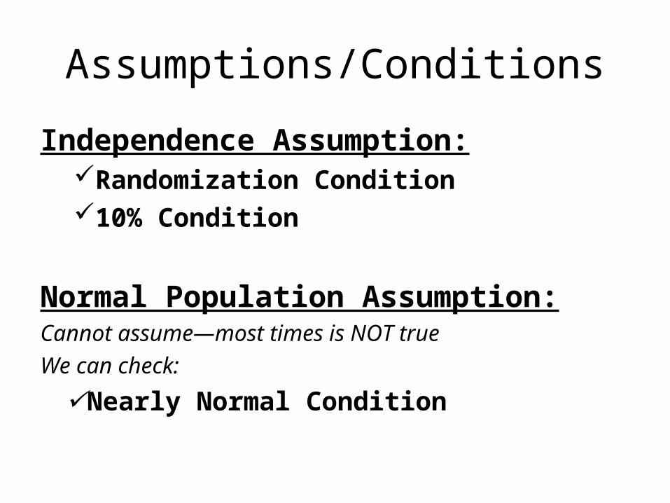
Independence Assumption:Randomization Condition10% Condition

Normal Population Assumption:Cannot assume—most times is NOT true

We can check:

Nearly Normal Condition

Nearly Normal Condition

To Check this condition, ALWAYS DRAW A PICTURE, EITHER A HISTOGRAM OR A NORMAL PROBABILITY PLOT.

Normality of t-model depends of sample size (think Central Limit Theorem).

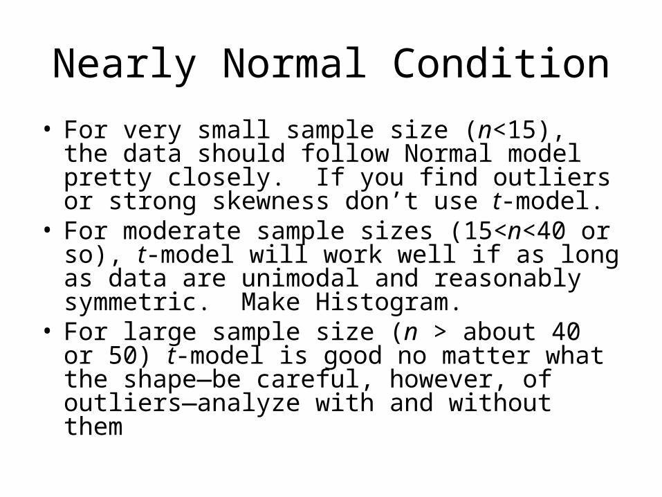
Nearly Normal Condition

• For very small sample size (n<15), the data should follow Normal model pretty closely. If you find outliers or strong skewness don’t use t-model.

• For moderate sample sizes (15<n<40 or so), t-model will work well if as long as data are unimodal and reasonably symmetric. Make Histogram.

• For large sample size (n > about 40 or 50) t-model is good no matter what the shape—be careful, however, of outliers—analyze with and without them

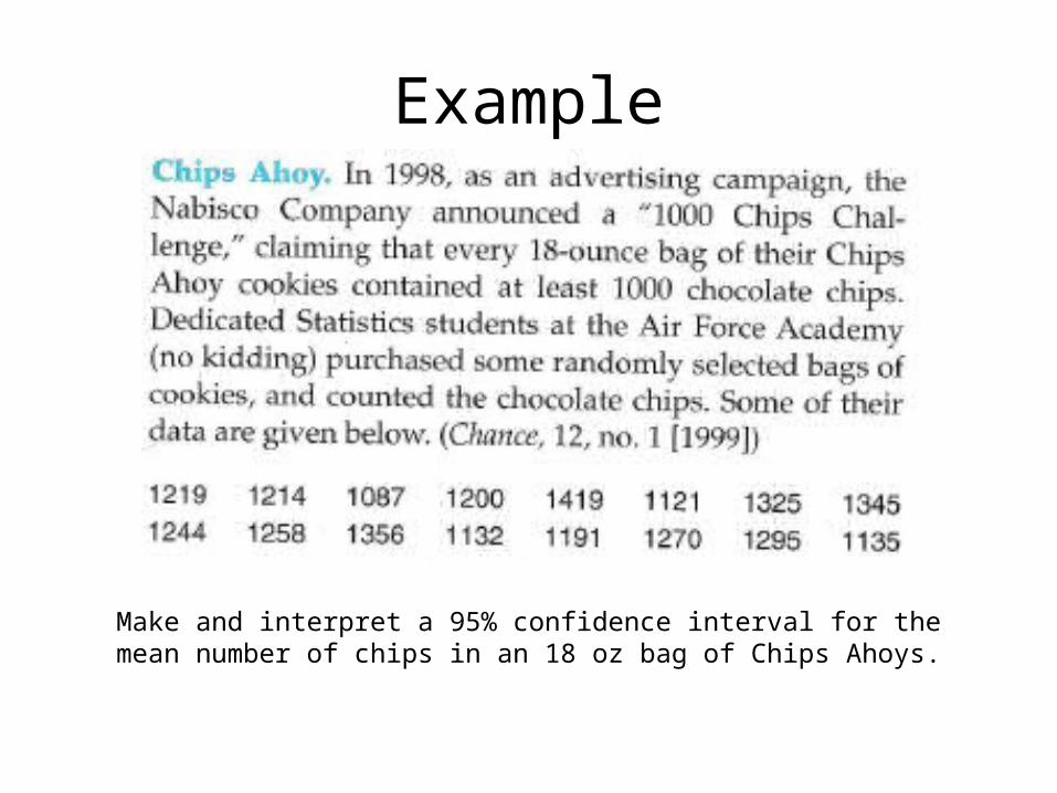
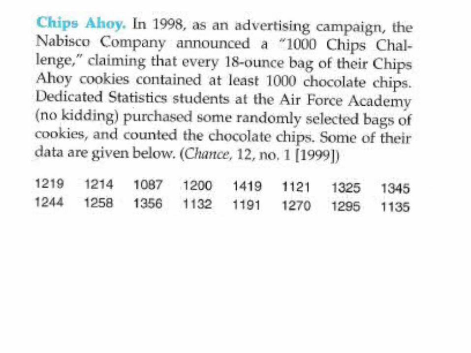
Example

Make and interpret a 95% confidence interval for the mean number of chips in an 18 oz bag of Chips Ahoys.

Check Conditions

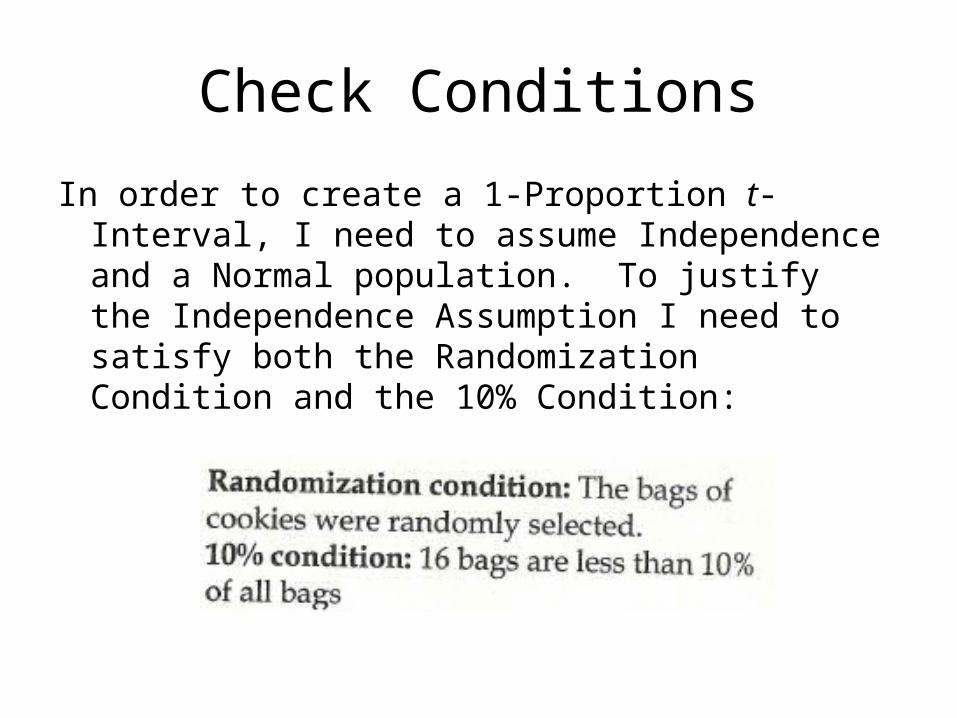
In order to create a 1-Proportion t-Interval, I need to assume Independence and a Normal population. To justify the Independence Assumption I need to satisfy both the Randomization Condition and the 10% Condition:

Check Conditions

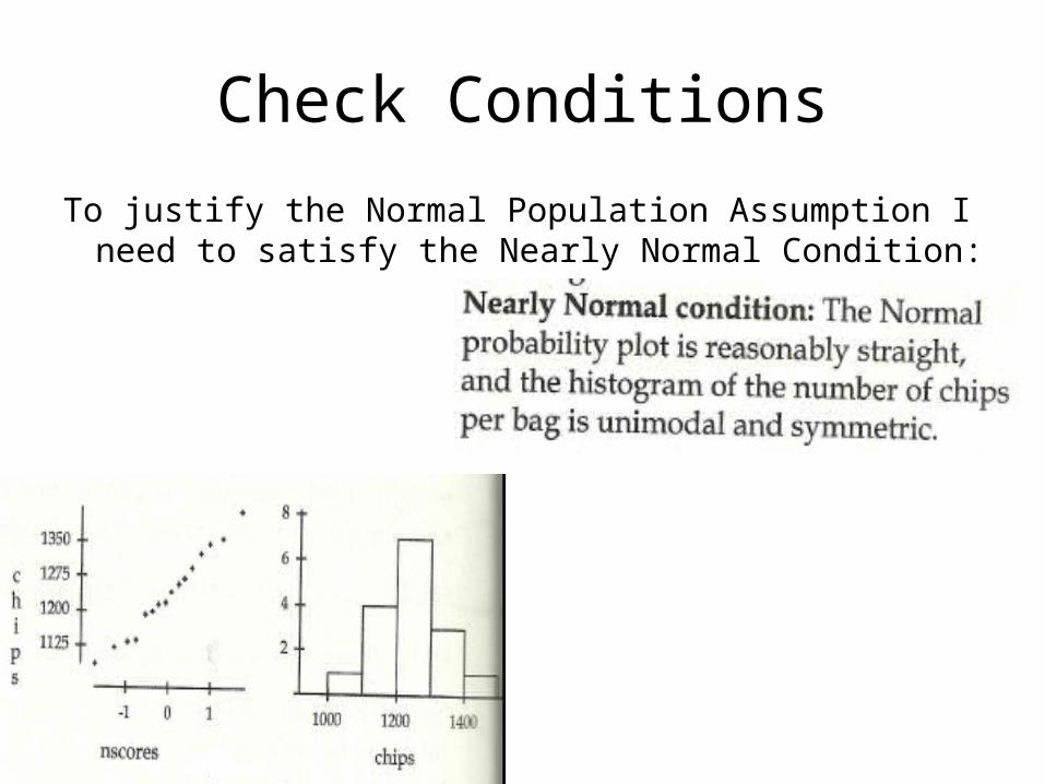
To justify the Normal Population Assumption I need to satisfy the Nearly Normal Condition:

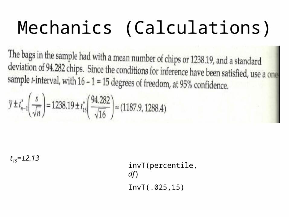
Mechanics (Calculations)

t15=±2.13invT(percentile, df)

InvT(.025,15)

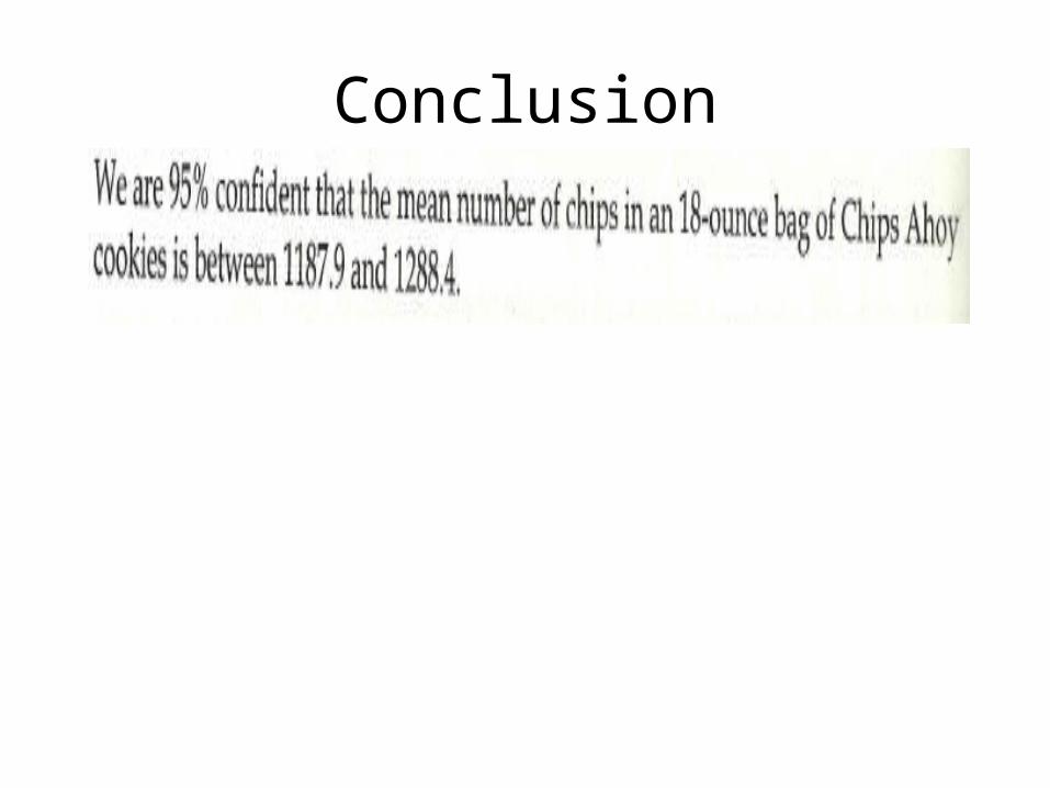
Conclusion

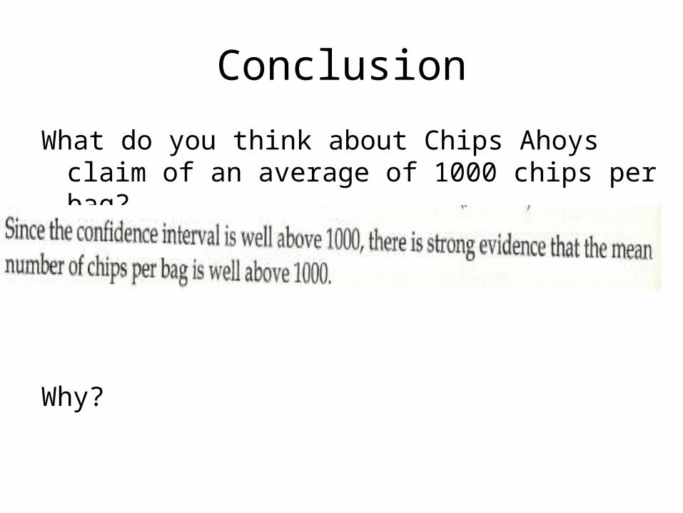
Conclusion

What do you think about Chips Ahoys claim of an average of 1000 chips per bag?

Why?

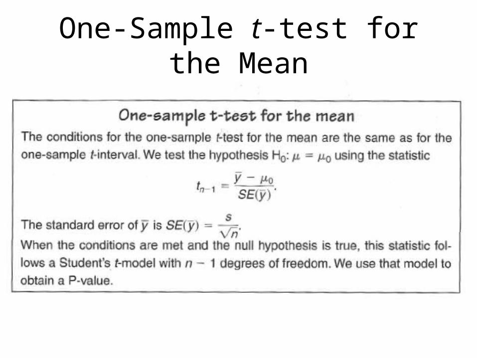
One-Sample t-test for the Mean

One-Sample t-test for the Mean

• A one-sample t-test is performed just like a one-proportion z-test.

• Use the 4 steps used in a test for proportions—the only thing that changes is the model. Instead of a Normal Model and z-scores, you use a t-Model and t-scores.

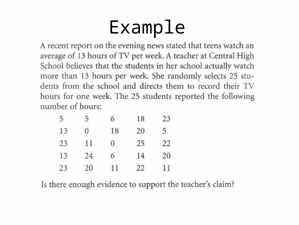
Example

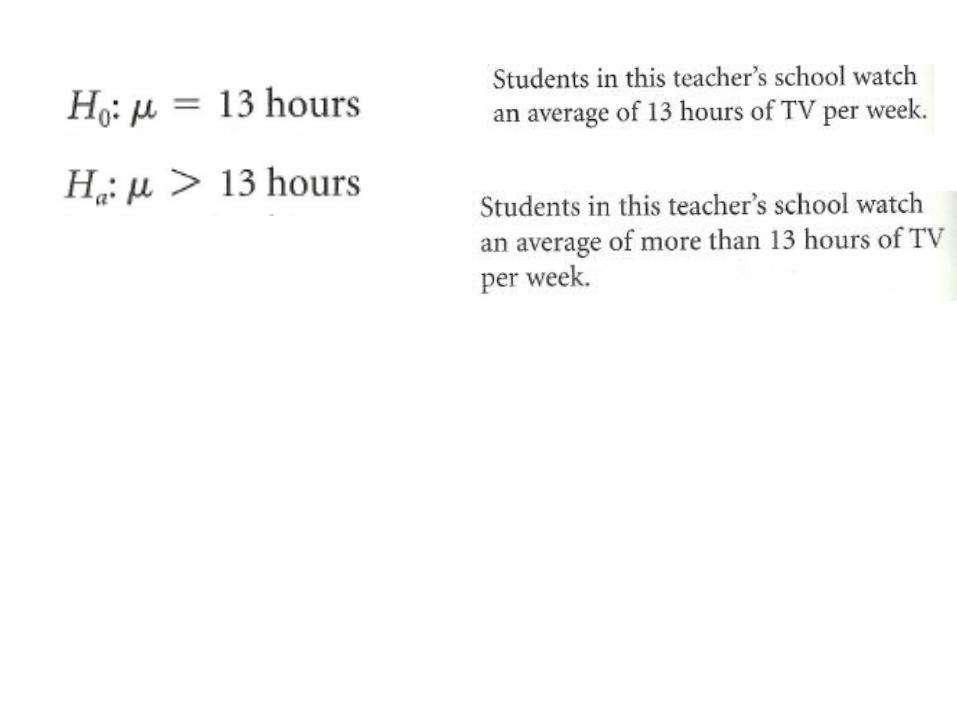
In order to conduct a one-sample t-test, I need to assume Independence and a Normal population. To justify the Independence Assumption I need to satisfy both the Randomization Condition and the 10% Condition:

Randomization Condition: It states that the sample was chosen randomly.

10% Condition: The 25 students represent less than 10% of all the students in the school.

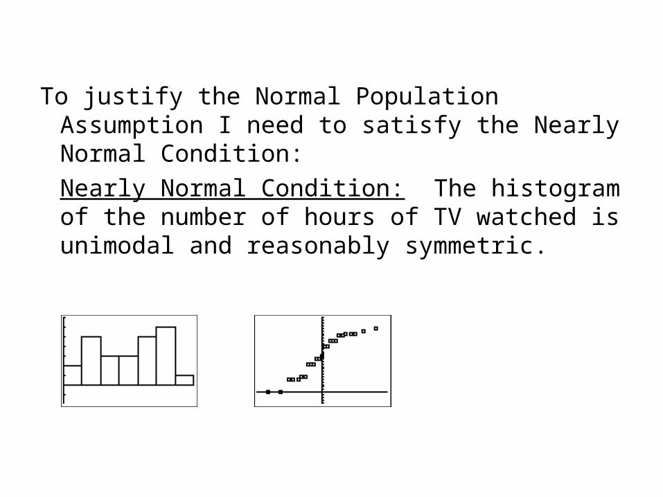
To justify the Normal Population Assumption I need to satisfy the Nearly Normal Condition:

Nearly Normal Condition: The histogram of the number of hours of TV watched is unimodal and reasonably symmetric.

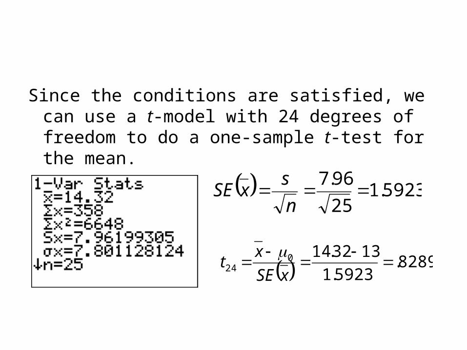
Since the conditions are satisfied, we can use a t-model with 24 degrees of freedom to do a one-sample t-test for the mean.

5923.125

96.7

n

sxSE

8289.5923.1

1332.14024

xSE

xt

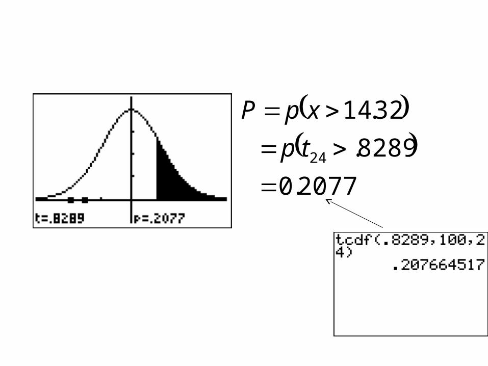
2077.0

8289.

32.14

24

tp

xpP

Given a P-value of 0.2077, I will fail to reject the null hypothesis at α=0.05. This P-value is not small enough for me to reject the hypothesis that the true mean number of hours that the students in this high school watch TV is 13 hours. Therefore, the difference between the observed mean of 14.32 hours and 13 hours is probably due to random sampling error.

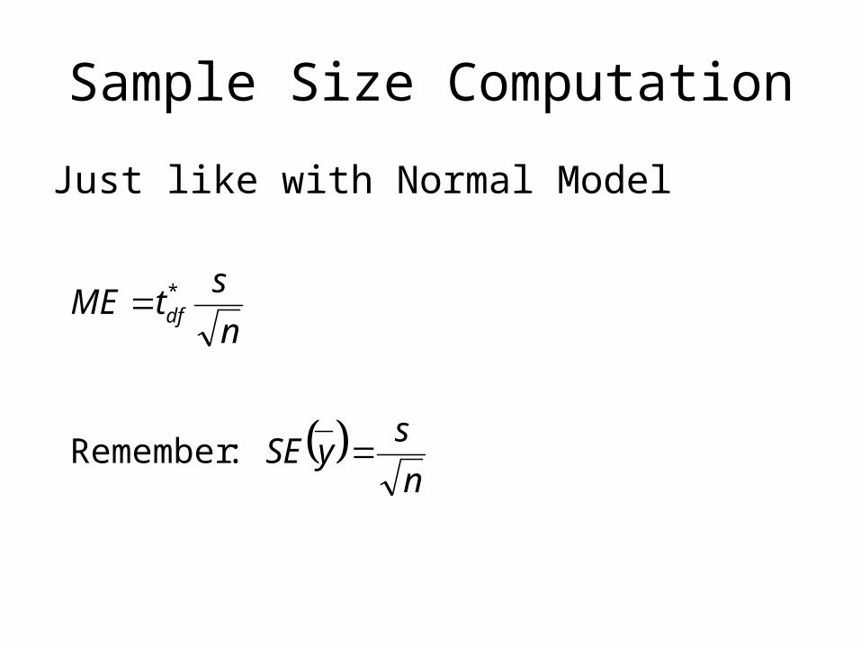
Sample Size Computation

Just like with Normal Model

n

sySE

n

stME df

:Remember

*

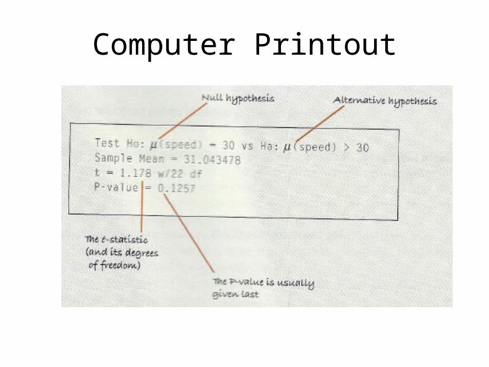
Computer Printout

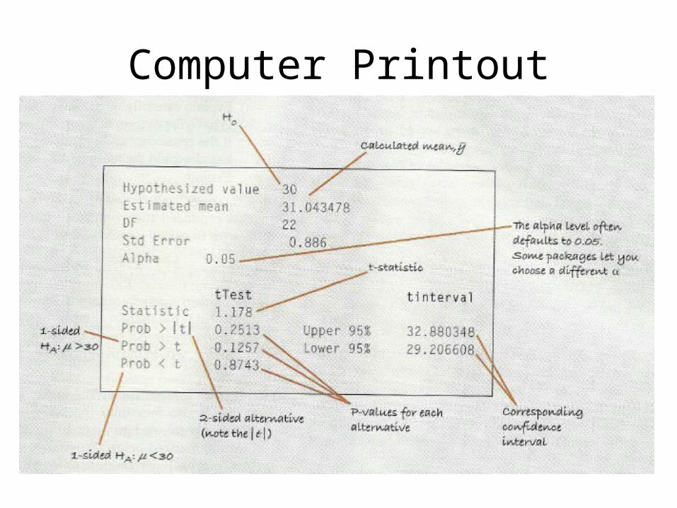
Computer Printout